
Numerical Modeling of Venturi Flume


1
Department of Civil Engineering, University of Ottawa, 75 Laurier Ave E, Ottawa, ON K1N 6N5, Canada
2
Department of Civil Engineering, Inonu University, 44280 Malatya , Turkey
*
Author to whom correspondence should be addressed.
Hydrology 2021, 8(1), 27; https://0-doi-org.brum.beds.ac.uk/10.3390/hydrology8010027
Submission received: 21 December 2020
/
Revised: 29 January 2021
/
Accepted: 1 February 2021
/
Published: 4 February 2021
(This article belongs to the Special Issue Advances in Flow Modeling for Water Resources and Hydrological Engineering)
Abstract
:In order to measure flow rate in open channels, including irrigation channels, hydraulic structures are used with a relatively high degree of reliance. Venturi flumes are among the most common and efficient type, and they can measure discharge using only the water level at a specific point within the converging section and an empirical discharge relationship. There have been a limited number of attempts to simulate a venturi flume using computational fluid dynamics (CFD) tools to improve the accuracy of the readings and empirical formula. In this study, simulations on different flumes were carried out using a total of seven different models, including the standard k–ε, RNG k–ε, realizable k–ε, k–ω, and k–ω SST models. Furthermore, large-eddy simulation (LES) and detached eddy simulation (DES) were performed. Comparison of the simulated results with physical test data shows that among the turbulence models, the k–ε model provides the most accurate results, followed by the dynamic k LES model when compared to the physical experimental data. The overall margin of error was around 2–3%, meaning that the simulation model can be reliably used to estimate the discharge in the channel. In different cross-sections within the flume, the k–ε model provides the lowest percentage of error, i.e., 1.93%. This shows that the water surface data are well calculated by the model, as the water surface profiles also follow the same vertical curvilinear path as the experimental data.
Keywords:
venturi flume; CFD; OpenFOAM; RANS; turbulence model; numerical simulation; Parshall flume1. Introduction
The Parshall flume is a simple static measuring device with no moving parts that is used to determine the flow rate in an open channel where a constant recording of discharge is required. The initial idea by Ralph Parshall in designing the Parshall flume was to make it easier for water users, like farmers, who do not have access to sophisticated types of equipment, to be able to determine how much water is delivered to them with an acceptable level of accuracy [1]. Currently, Parshall flumes are mainly used in irrigation and sewer systems to measure the flowrate [2]. In general, they are designed to generate a critical flow within the throat section, which affects the water level along the converging section upstream, implementing an empirical relationship between water surface elevation and discharge results in finding the discharge value at a specific time from the water surface elevation.
Variations of Parshall flumes are typically restricted to the dimensions of the geometries proposed by Ralph Parshall in 1936 for limited size numbers, i.e., 16 sizes, which vary in the opening from 1” to 144”. The arbitrary dimensions of the flumes used in various open channels in recent years have not been comprehensively studied. Since then, technology has advanced significantly, especially in the development of computational tools. Numerical simulations have introduced a new revolutionary chapter to the design of hydraulic structures, allowing engineers to extend their full potential by designing a variety of different hydraulic structures with new arrangements in their dimensions and shapes. They allow designers to optimize the specifications of their design to suit the need of the project’s objective. Computers and modeling software offer possibilities to perform extensive calculations, and they allow new designs to be tested with relatively low cost. For instance, a proposed hydraulic structure can be simulated to study its behavior under working conditions. This provides engineers with extensive variations in geometries and dimensions when designing a structure. Using computer models makes it possible to implement Parshall flumes with complex shapes and dimensional limitations where needed.
The authors of [3] used a numerical model to develop an alternative rating equation to be implemented at low discharge for different flume sizes. In a study on a submerged Montana flume, to prove the reliability of the CFD programs’ accuracy, the flow rate was calculated with FLOW- 3D. It is shown that the numerical results closely matched the experimental results. Furthermore, it is revealed that a free-flow equation for a Parshall flume would also be a good fit for a Montana flume [4]. To determine the accuracy of a field-scaled Parshall flume at a wastewater system in Minneapolis, Minnesota, [5] implemented the large-eddy simulation (LES) and level-set method to compute the turbulent flow under two-phase flow conditions. A three-dimensional finite difference code, SOLA-FLUMP, is presented by [6] to assess the various effects due to the sloped channel, the upstream velocity profile distortion, and the geometry of the flume.
A parametric study was performed in terms of stability and accuracy on Reynolds-average Navier–Stokes (RANS) and hybrid RANS/LES turbulence models and numerical schemes offered in openFOAM, an open-source software, by [7]. From the results, the second-order upwind scheme and limiters were found to be the most stable with the lowest computational cost, thereby providing the highest level of accuracy for RANS models.
It is important to determine the degree of reliability of the model that is going to be used for a specific simulation. One of the most dependable approaches is to evaluate the simulated results with actual experimental data. In this paper, different simulated datasets generated from seven dissimilar methods, i.e., standard k–, RNG k–, realizable k–, and k– SST; large-eddy simulation (LES); and detached eddy simulation (DES) are examined versus four physical datasets obtained from physical experiments on different flumes with different discharges.
A high-order partial differential equation, like the momentum transport equation, that includes nonlinear terms cannot be solved analytically to obtain a general solution. Numerical solutions require discretization techniques to reshape the continuous partial differential equation into a discrete equation. Computational fluid dynamics (CFD) using the finite volume method (FVM) [8] can be very useful for this purpose. With the rapid increase in the computational capability of computers, large-eddy simulation (LES) is increasingly embedded in the CFD models used by researchers and engineers to solve turbulent flows [9]. LES is a compromise between the efficiency of Reynolds-average Navier–Stokes (RANS) and the prohibitive computational cost of direct numerical simulation (DNS). Approaches of LES or the variant hybrid family like RANS/LES (DES) are progressively taking over the computationally expensive DNS approach to solve problems with compound geometries and flow properties [10].
The authors of [11] tried to introduce a correction coefficient to a 24” Parshall flume where the positions of the staff gauges were mislocated and the condition of the flume entrance was set up differently from the one introduced by [1]. They used numerical modeling to implement the correction factor for other sizes of Parshall flumes. Based on this study, a part of the small deviations, the physical model, and numerical simulation were aligned with one another.
In order to decrease the head loss in a curved flume, three flumes were studied on the basis of critical flow by [12]. The study was conducted on laboratory experimental results versus numerical simulation data. The hydraulic parameters such as velocity of the free surface and the depth of water were analyzed and compared. A maximum error of 4.7% in the water depth was obtained. It was shown that a good consistency was achieved between numerical simulation and experimental data.
The objective of this paper is to solve the Navier–Stokes equations using OpenFOAM to study the behavior of various numerical models in simulating Parshall flumes similar in size and flowrate to the flumes used in physical experiments by Dursun (2016).
Based on the literature review at the beginning, there is no comprehensive numerical solution that has been conducted on the models simulating the hydraulic structures, i.e., Parshall flume. The reliability of RANS LES and DES turbulence models in simulations has been studied in this research by evaluating the performance of seven turbulence models against the experimental data of different Parshall flume structures. Subsequently, the consistency of the simulations was determined in various scenarios in relation to the experimental data. Based on what was discussed in the literature review, seven turbulence models, i.e., RAS models (including standard k–ε, RNG k–ε, realizable k–ε, and k–ω SST) and hybrid RANS/LES models (such as k–ω, SST-DES, and an LES models, namely, the Smagorinsky method and dynamic K LES method), respectively, were selected due to their wide usage and advantages compared to other turbulence models.
This paper is organized as follows: the methodology is explained in the next section, including governing equations, turbulence models (including RANS, LES, and DES models), numerical setup (including initial and boundary conditions), mesh analysis, and data; the results and discussion are then presented, in which the performance of numerical models is discussed. Some concluding remarks complete the study.
2. Methodology
By the increasing power of processors, computational fluid dynamics (CFD) has become the most convenient tool to simulate fluid motion. In CFD, the fluid’s flow establishment follows physical parameters, including pressure, viscosity, velocity, and temperature. In order to simulate a physical case related to the fluid flow, the physical properties should be taken into account accurately.
CFD approaches are used in solving the fluid flow equations as well as fluid interaction with solid bodies. The Euler equation for inviscid fluid and the Navier–Stokes equation for viscous fluid can be derived in their integral arrangement with respect to the conservation of energy, mass, and momentum [13].
OpenFOAM is one of the open-source solvers for CFD that is widely used for simulations. It is a platform including numerous C++ libraries and applications that are able to solve numerically the continuum mechanics problems [14]. It uses a tensorial method that implements an object-oriented programing approach and employs the finite volume Method (FVM).
2.1. Governing Equations
A viscous incompressible fluid flow is governed by a general three-dimensional system of equations, called the Navier–Stokes system, that consists of momentum and continuity equations. The system is described as follows [15,16]:
where ρ denotes density; p represents total pressure; u, v, and w represent the velocity in three different directions, i.e., x, y, and z; t is used for time; and gravitational acceleration is denoted by ρ is obtained using the following equation:
Here, ρ1 and ρ2 represent the air and water densities, the two phases of the involved fluid. The value varies from 1 to 0 depending on the location, where 1 denotes the presence of water and 0 shows the presence of air. Any number between these two values represent the interface.
Finally,
2.1.1. Equation of the Free Surface
With respect to the zero pressure at the surface, the free surface was analyzed with the volume-of-fluid (VoF) method. The following equation is used by VoF:
As stated earlier in this paper, a powerful open-source CFD, i.e., OpenFOAM application, was used for the purpose of the numerical simulations.
The flow motion in a Parshall flume was simulated in this study with the help of seven different turbulence models: standard, realizable, and RNG k–ε models; k–ω SST models; and detached eddy simulation (DES) models, such as k–ω SST-DES; as well as LES methods, including the Smagorinsky LES model and dynamic K LES model. In the following, a brief description of each selected model is provided.
2.1.2. Reynolds-Average Navier–Stokes (RANS) Approach
The Reynolds-average Navier–Stokes Model is currently the most popular approach for the simulation of fluid flow. This approach essentially uses a viscosity term to approximate the turbulence equations. K is a term in these models that represents the fluctuations of the turbulence kinetic energy per unit mass.
Standard k–ε Model
This model requires two additional transport equations: one for turbulent kinetic energy and another for energy dissipation . Apart from its poor performance in large adverse pressure gradient cases, it is known as one of the most popular turbulence models [17]. This model comes from the Reynolds-averaged Navier–Stokes (RANS) category where modeling is applied to all properties of fluid motion.
The equation for turbulent kinetic energy and dissipation is shown below:
is the component that controls the turbulence scale where represents the turbulence kinetic energy. The reader is referred to [15] for further details and values of the coefficients.
Realizable k–ε
The latest improved form of the three k-epsilon models is the realizable k-epsilon model [18,19]. There are two significant differences when this model is compared to the standard k-epsilon model. Firstly, formulation of the turbulence viscosity has been revised. Secondly, the dissipation rate transport equation is explained based on the equation of transport of the mean-square vorticity [19,20].
The reader is referred to [21] for further details and value of the coefficients.
2.1.3. LES Approach
Smagorinsky LES Model
This model was originally developed within the metrological community to simulate atmospheric air currents [22]. As a well-known subgrid-scale model according to [23], the Smagorinsky model estimates the shear as
where
The reader is referred to [22] for further details and values of the coefficients.
One of the main disadvantages of this model is the lack of ability to predict the energy transfer from subgrid-scale structures to the greater resolved scales; thus, the model is totally dissipative. Another problem with the Smagorinsky model is that its coefficient has to be adjusted for every flow field. However, it is still one of the well-known models in the field of CFD. The Smagorinsky model is easy to use in numerical simulations. If the Smagorinsky coefficient is adjusted based on the local characteristics of the fluid motion, it can generate more accurate results [23].
The Dynamic One-Equation Model
The SGS stresses determine how successful an LES model can be. As a simple model, in the Smagorinsky model, the factor of the proportionality is a fixed value that has to be determined before running the model. In reality, the factor is a flow-dependent value and is not defined as a single universal constant. The weak point of the model comes from this section. There have been attempts to improve this model [24,25]. Moreover, this model is completely dissipative, and there is always a transformation of large-to-small scale for the energy.
On the other hand, dynamic models are the best choice to substitute the Smagorinsky model. In this model, the value of the subgrid eddy viscosity is determined while the simulation is computed [26]. In recent decades, a one-equation dynamic model has been presented [27]. The equation of the dynamic model is presented below.
where the and coefficients are derived from local flow properties [21]. The reader is referred to [28] for further details.
2.1.4. DES Approach
k–ω SST-DES
While the RANS model is derived through Reynolds temporal averaging, the LES model is the result of spatial filtering. Between these two methods, the difference is the magnitude of the generated eddy viscosity. This is one of the main reasons for the development of the DES model, which has the ability to cover the weaknesses of LES when it comes to treating wall regions with very fine mesh [29].
The RANS approach is used in the near-wall region by the DES method where, at the same time, the LES model is applied to the rest of the region excluding the wall region. The region associated with the LES model is usually the core turbulent area, where large-scale turbulences play a major role. Within this area, the DES approach uses a LES subgrid-scale model, while for the near-wall region, it uses the RANS model [30].
A DES-improved form of the k–SST method is the k–SST DES approach [31,32]. Recently, in the aerodynamic field, DES has been widely implemented due to its computational speed and quality of results. It is proven to be less computationally expensive, and it generates better results than steady RANS [33,34].
The turbulence specific dissipation rate equation is given by
and the turbulence kinetic energy is calculated as
the length scale, , is given by
and the turbulence viscosity is obtained using
The reader is referred to [35] for further details and value of the coefficients.
2.2. Numerical Setup
2.2.1. Numerical Solution Details
The combination of the finite volume method with the VoF method was used in the model. To solve the governing equation of motion, the “interFoam” solver was implemented in OpenFOAM. The temporal term was discretized with the help of a Eulerian scheme, besides the Gauss linear method, which is used for the gradient term. For the Laplacian, the corrected Gauss linear method was applied. The divergence terms were discretized using a Gauss vanLeer plus Gauss linear scheme. The linear scheme was used to discretize the interpolation term.
The tolerance level was defined for each individual variable, while the desired convergence was expected to be achieved where an iterative solver was used in the processing. The Gauss–Seidel technique was applied with a level of accuracy of for the fraction of liquid , for pressure, and for the velocity.
2.2.2. Initial Conditions
The flume had a fixed inlet flow velocity for each case, i.e., a discharge of 20 L/s or 30 L/s as the initial conditions. There was no initial acceleration or dissipation defined in the model. There was no flow across the walls, i.e., there was no liquid coming in or getting out through the wall boundaries at the defined locations. Initial water surface was set to be constant everywhere.
2.2.3. Boundary Conditions
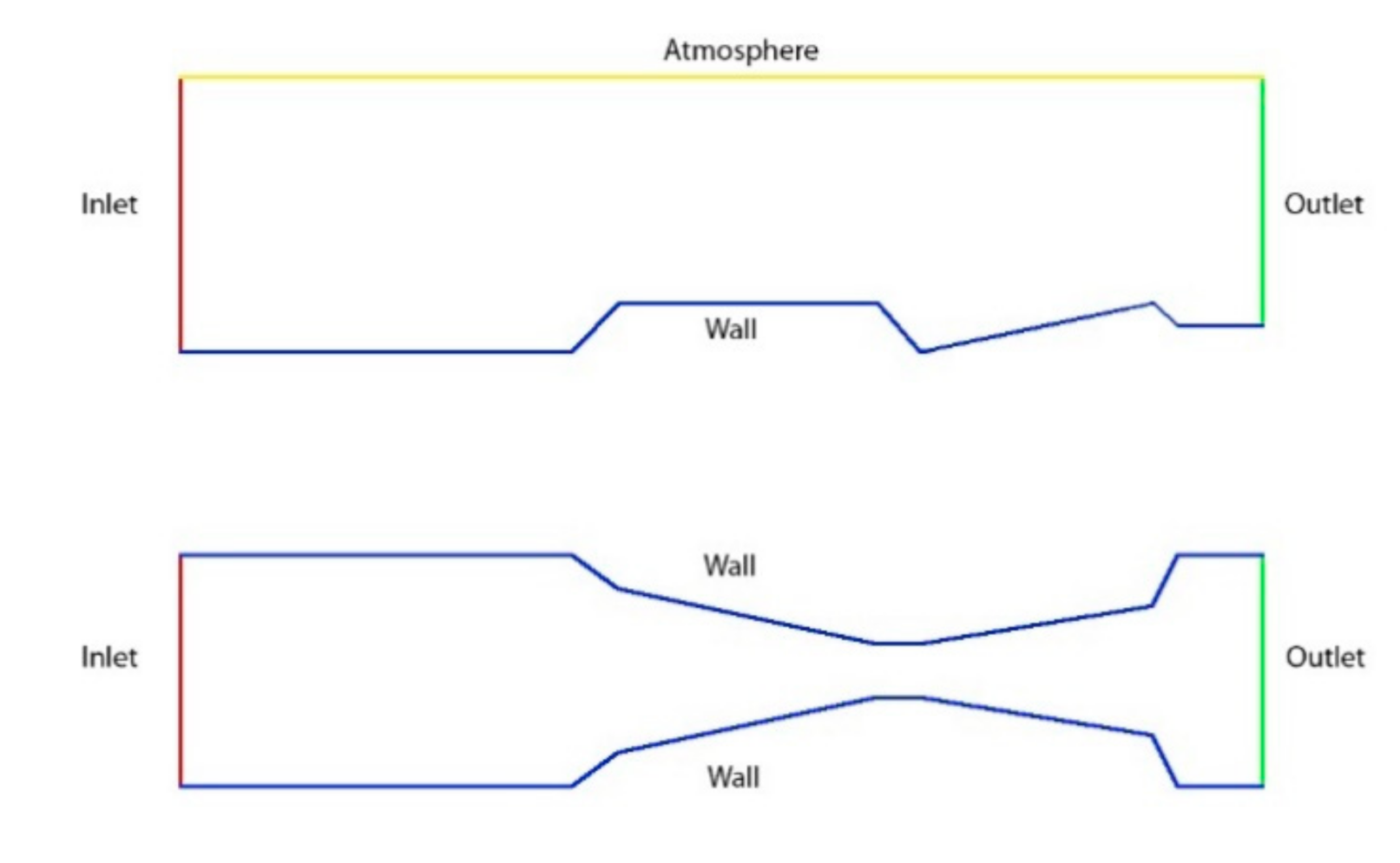
There were different boundary conditions employed in this simulation as illustrated in Figure 1. Hydraulically smooth walls were considered in this study, and standard wall functions were employed. Water discharge was specified at the inlet. Zero gradient condition was considered at the outlet. The free surface was tracked based on the volume-of- fluid method based on a zero pressure condition at the interface of air and water. Figure 1 below shows the boundary segments from the side view and top view of the simulated Parshall flume.
2.2.4. Mesh Analysis
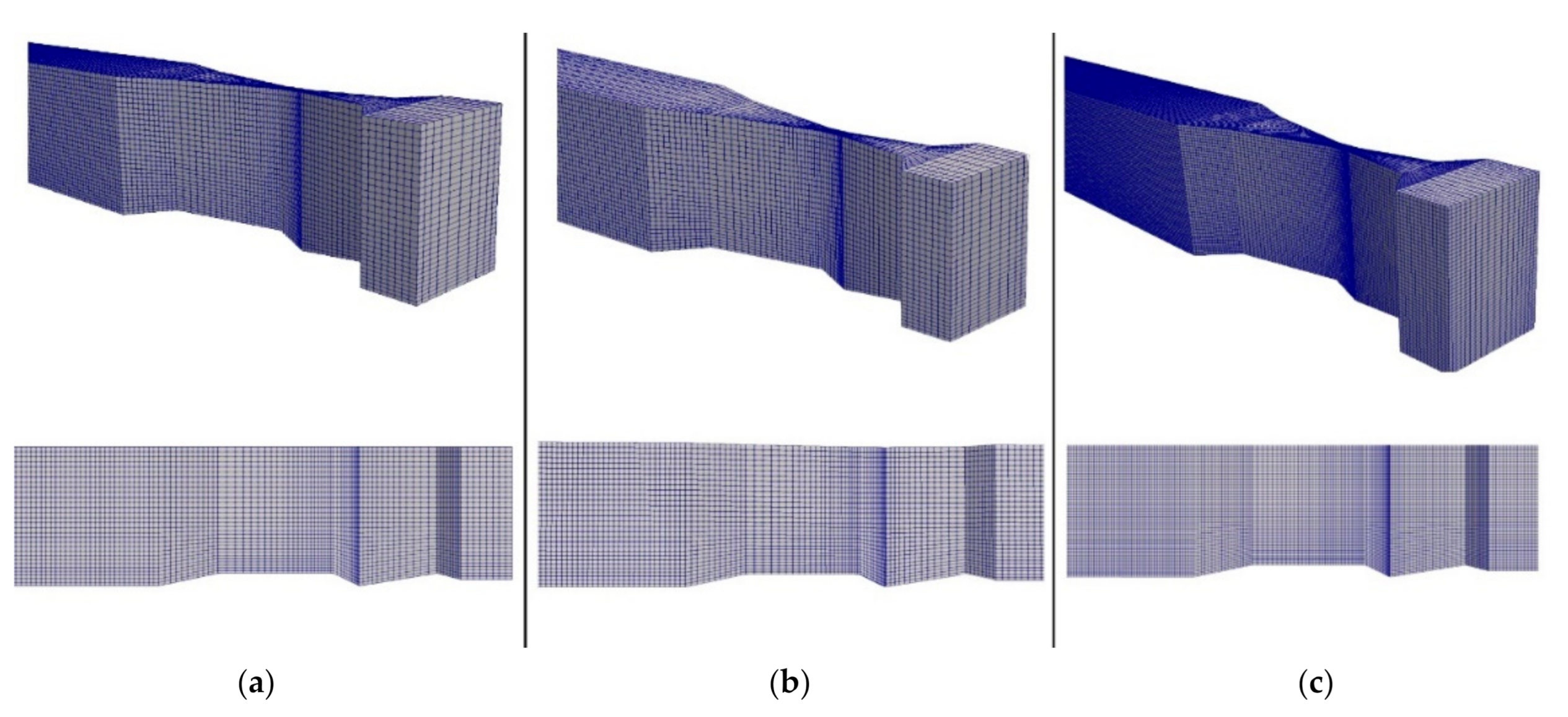
In this study, in order to determine the optimum size of the mesh, mesh sensitivity analysis was conducted. The mesh grid used in this paper is a structured mesh. The purpose of this analysis is to find the finest mesh size for which the results will not be affected further.
Figure 2 shows the mesh sensitivity analysis performed on the Parshall flume. The maximum cell number was 263,700 cells for this structure. The optimal case in terms of computational cost and changes in results is that illustrated in Figure 2b, with a total of 74,496 cells. Greater reduction applied on the cell size did not significantly change the numerical results.
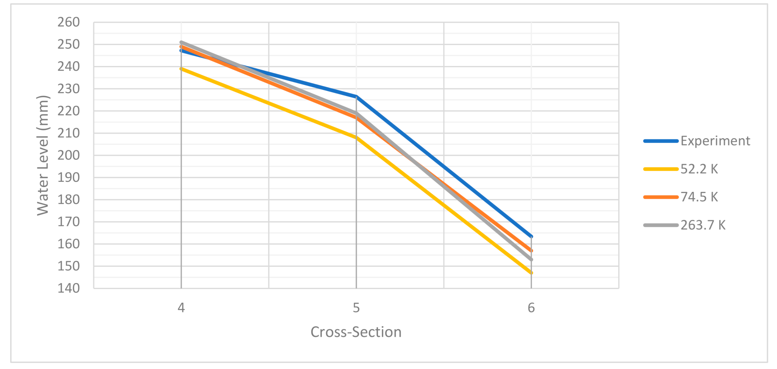
In Figure 3, the results of the mesh sensitivity analysis are provided for the cross-sections 4–6. As the size of the original coarse mesh became finer, the simulated water levels approached the values of the experimental data. In this study, the initial number of cells was 52,200, and it was gradually increased to 74,496 and further to 263,700 cells. The results from the last two finer meshes show negligible difference; hence, the mesh containing 74,496 cells was selected and further used to implement the remaining turbulence models.
2.2.5. Data
The experimental tests were conducted in the hydraulic laboratory of Firat University, Elazig, Turkey (Dursun, 2016). The tests were performed in a rectangular channel with the dimensions of 0.4 by 5 by 0.6 m in width, length, and depth, respectively. The purpose of these experiments was to determine the changes in the quantity of the dissolved oxygen of the stream before and after a Parshall flume structure was introduced. The dimensions of the Parshall flumes that was used in this research were the same as the 3-inch (7.62 cm) Parshall flume with a 45 degree wing wall. The discharge in the experiment was measured using an electromagnetic flow meter.
The model was run for 300 time-steps where, after 120 steps, water levels became steady; water surface fluctuations, for instance, were limited to +/−0.003 m. The water level is shown using a post-data analysis software called ParaView. At the point of interest, two vertical planes (perpendicular to each other) were introduced, where the intersection line between the two planes was set to pass the desired point. The Y-coordinate (water level) of the line was extracted using the calculator filter; for example, the water level at each desired time step is shown afterwards in the tabulated mode in a separate window in ParaView.
3. Results
The numerical simulation for the experimental case conducted by [2] is performed in this study. The Parshall flume used in this study is a 3-inch Parshall flume modified to meet the experimental criteria. OpenFOAM was used as an open source CFD tool to carry out the numerical simulation of the Parshall flumes.
Switching from a coarse size mesh grid to a finer grid size in the mesh sensitivity analysis led to some change seen in the numerical simulation model results. As the flow rate decreased from 30 to 10 L/s, the model tended to produce better results. This pattern is observed in the model as well as the other RANS models.
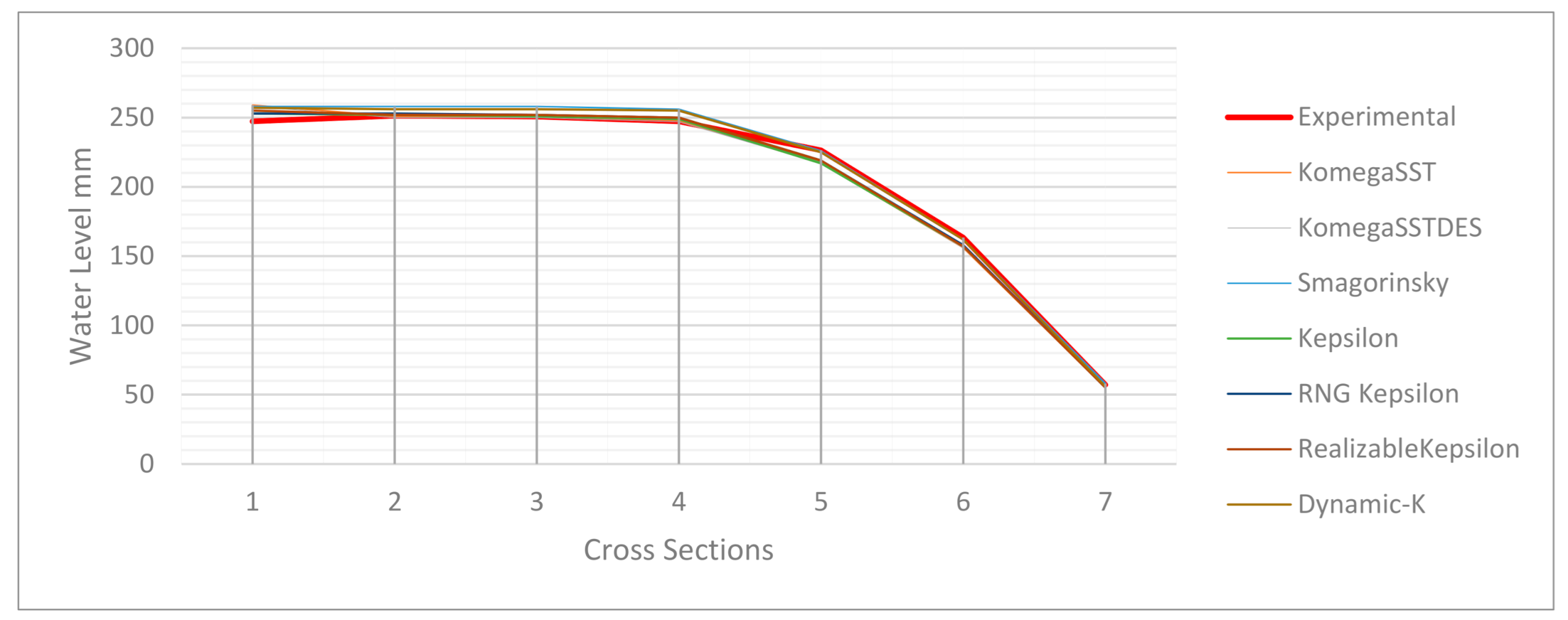
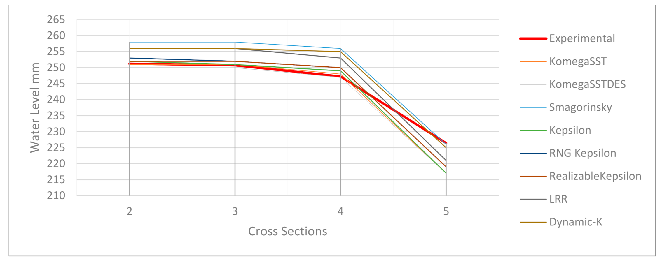
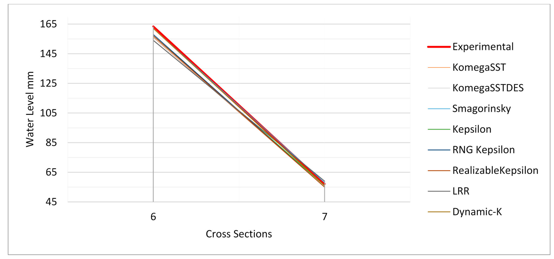
Water surface elevations in seven cross-sections were compared with the experimental results with three different flowrate values, i.e., 10, 20, and 30 L/s. Figure 4 shows water surface elevation for the flowrate of 10 L/s using seven various models. As shown in Figure 4, all models follow the same pattern as the experimental data. Figure 5 and Figure 6 are introduced to show more clarified view of the water level data. Based on the results of various turbulence models used in simulations, the k–ε turbulence model provides the most accurate simulation compared to the other models used in this study.
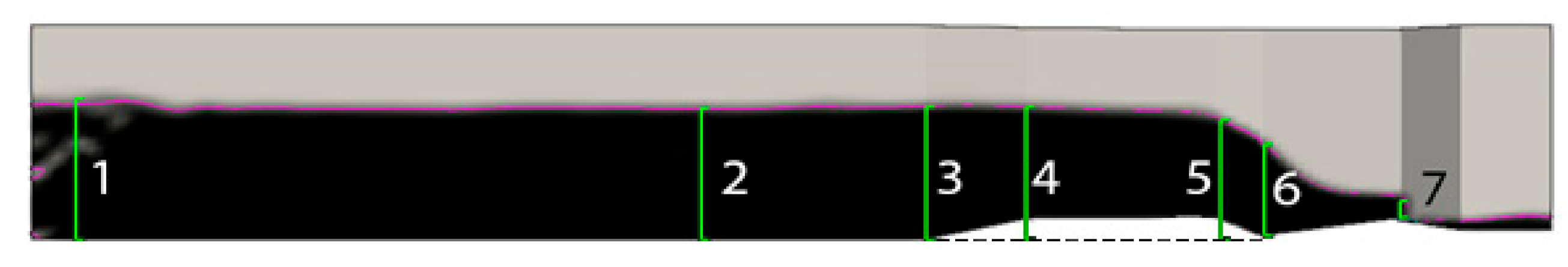
The locations of the cross-sections in the Parshall flume are denoted in Figure 7 where at all critical locations, a cross-section is introduced. The reason for choosing the cross-section locations, as shown in Figure 7, is that in the laboratory experiment conducted by Dursun in 2016, the same locations were chosen; hence, water level data were also available for them.
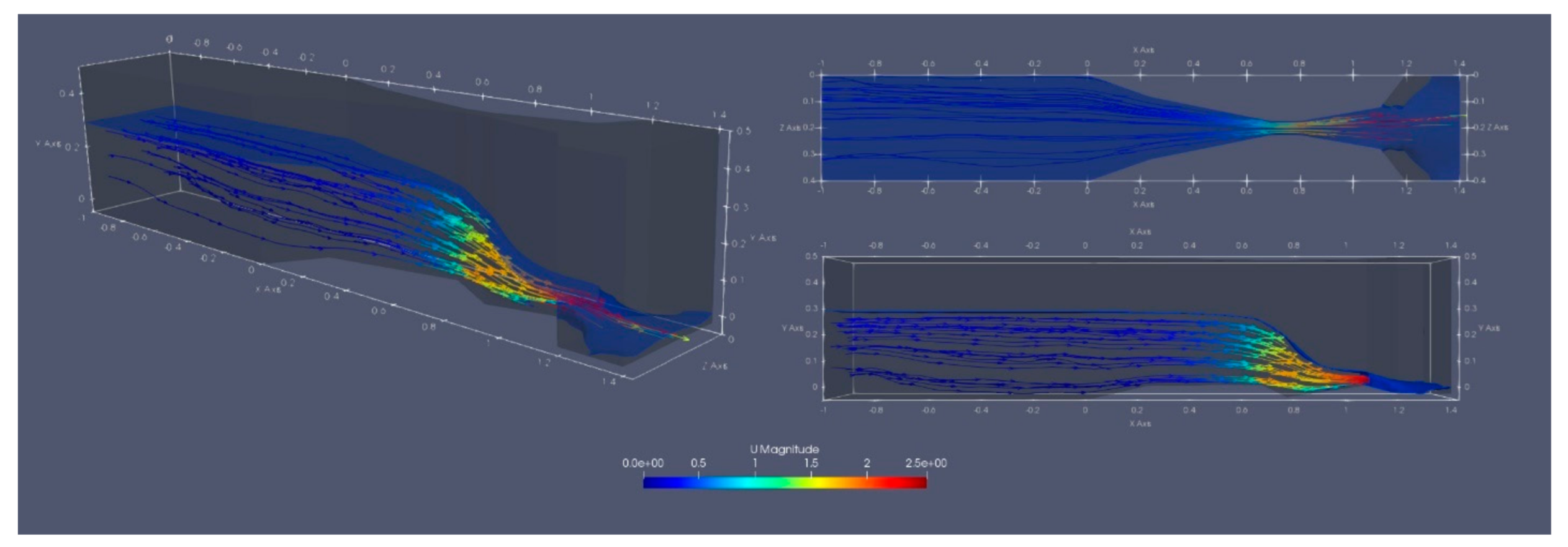
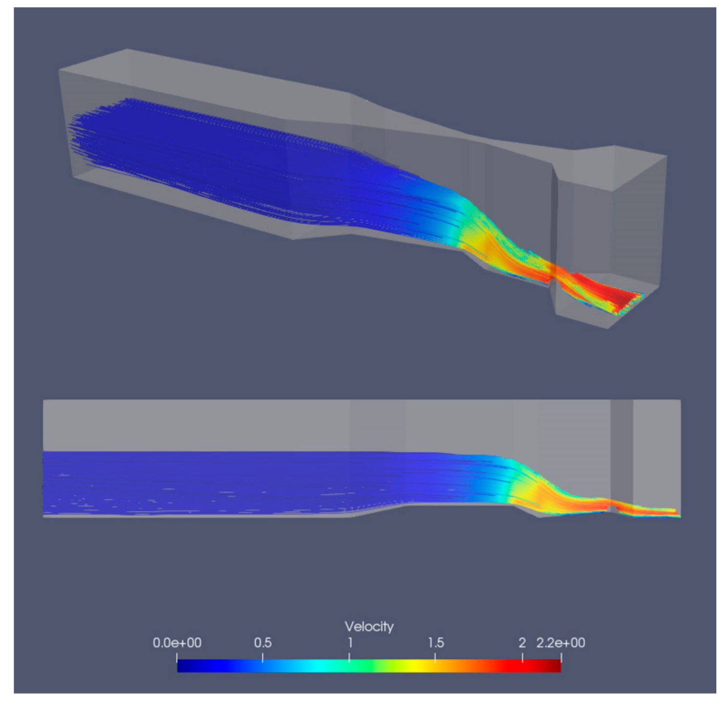
In Figure 8, the fluid flow in the Parshall flume with a flowrate of 10 L/s is illustrated. As the stream lines indicate, the velocity of the fluid prior to the flume throat displays a maximum of 1 m/s, and by the time it reaches the narrow section with a declining floor, the speed rapidly increases by 50%. This is the section where the fluid experiences supercritical flow. It continues to increase by the end of the divergence section where maximum velocity is reached (red arrows), i.e., 2 to 2.5 m/s. Once the fluid reaches the inclined slope in the divergence section downstream, the flume forces it to develop a hydraulic jump.
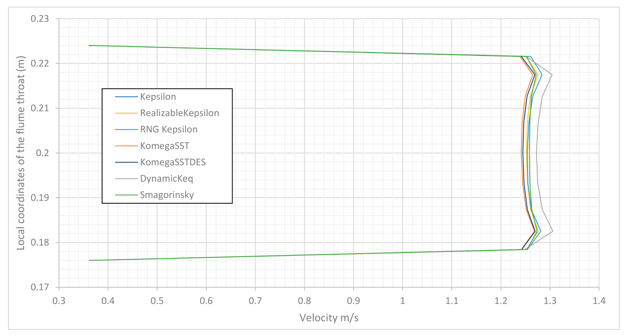
The velocity profiles of all seven turbulence models at cross-section 5, where the numerical models exhibited the maximum velocity, are shown in Figure 9. The comparison between different velocity profile shows that in the seven different turbulence models, the values are almost identical, with a difference margin of 0.04 m/s at the maximum velocity points. The maximum recorded velocity in the flume for different models is within the range of 1.26–1.28 m/s in the different models. The “y” axis is the local coordinate of the flume throat defined in the OpenFOAM computational domain.
As illustrated in Figure 10, the velocity is constant upstream of the midsection of the converging area. At the end of this section, the flow is forced to increase its velocity due to the narrow design of the throat combined with a sharply slopped bed. The velocity streamlines after the throat section of the flume show that the velocity magnitude is greater than that observed throughout the rest of the structure. Once the flow immediately exits the divergence section, it attains maximum velocity.
The flume’s pressure field is represented in Figure 11. In the section between cross-sections 5 and 6, the pressure is negative. As illustrated in this figure, due to the throat section, the pressure is built up in the upstream, while when passing cross-section 5 toward downstream, the value of the pressure drops rapidly.
4. Discussion
The percentage difference of water level values of the numerical models and the experimental data is specified in Table 1 below. The calculation is performed based on the following relationships [15]:
Here, the root mean square error (RMSE), centered root mean square error (CRMSE), and correlation coefficient (R) are used in order to compare the simulation results with experimental data. The results from the above formulas are presented in Table 1, where different types of error analysis are applied in order to determine the reliability of the numerical simulations.
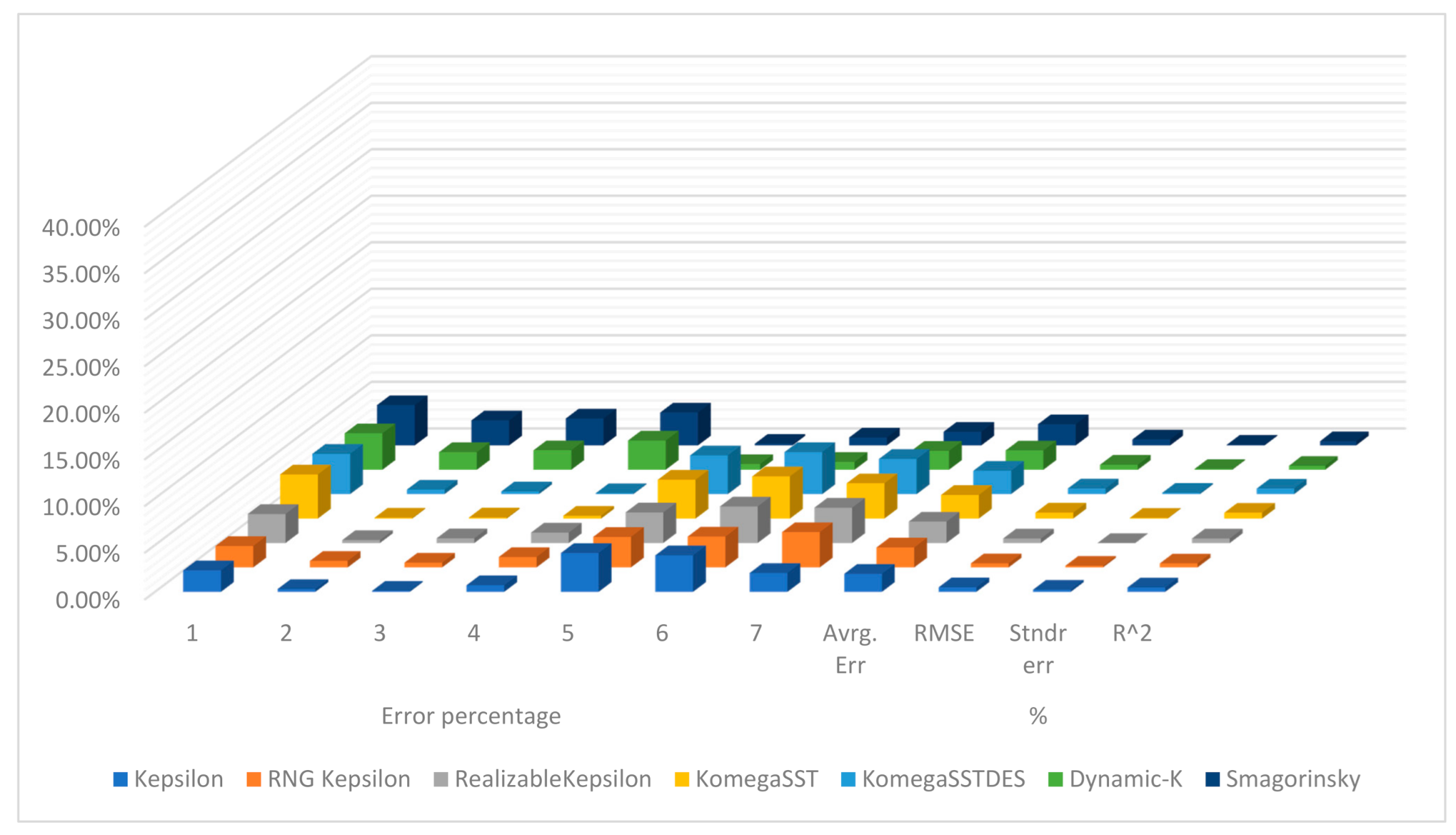
Among the seven different turbulence models applied in this study, the Smagorinsky and dynamic K equation models provide the least average error values. This model provides the minimum error percentages not only in the average value of all of the cross-sections but also within the first three, i.e., 1, 2, and 3.
By calculating the root mean square error for all the turbulence models, the results show that two models, and dynamic K LES, provide the lowest values, 1.93% and 2.08%, respectively, while the model has a greater value compared to the others. However, for comparison of the values of this turbulence model, the Smagorinsky and dynamic K LES models have the closest value to 1, i.e., 0.998.
The ranges of the average error percentage for all of the turbulence models are within a narrow domain a minimum value of 1.93% and a maximum value is 2.53%. While most of the turbulence models used in this study provided reliable error percentages, the model was the only one that generated results with a high average error of 2.53% and RMSE of 0.64%, and the lowest was also recorded for this model.
Table 1 and Figure 12 tabulate the results of the different numerical simulations at various locations in the flume, i.e., at the seven cross-sections. The average values and the statistical analysis that were discussed earlier in this section are also included here.
At cross-section 1, the error percentages for all the models were larger than those calculated at the next cross-section (cross-section 2). Since the location of the first cross-section was chosen very close to the defined inlet of the flume, the unsteady water surface affected the results at this point.
4.1. RANS Models
The best average performance was obtained using the standard k–ε turbulence model. The other turbulence models that fall into this family showed less accuracy than the LES models. However, the difference percentages at Sections 2–4 are better than those obtained using the LES and DES models.
4.2. DES Model
The only DES model used in this study, , provided almost the same average result as those obtained using the , which has the greatest average error percentage among the models. The second highest average error percentage was observed for the DES family of turbulence models.
4.3. LES Model
Two LES models were used in this study. The water surface elevation results from the Smagorinsky model and dynamic K LES are similar to those of the RANS model family. The average error value, as mentioned earlier, is the lowest for dynamic K LES following the standard k–ε model.
The pressure and velocity fields for all the models follow same pattern, where the low velocity of the flow is converted to supercritical flow just after entering the throat section of the flume. The pressure field exhibits opposite behavior as the initial high-pressure flow enters the throat of the flume: the pressure drops and reaches a negative value in the throat over a short distance.
At the sections where the velocity is locally maximum, the pressure value drops dramatically. This is due the higher viscous losses occurring with the high velocity flow.
5. Conclusions
The main objective of this study was the numerical examination of fluid motion in a Parshall flume. Assessing the results of different turbulence models, such as standard , realizable , RNG , SST, SST DES, Smagorinsky, and the dynamic K LES. reveals that despite some poor performance of within two cross-sections, the same as the rest of the turbulence models except DES family models, this method estimates the water level accurately enough overall.
This study shows that the results from a turbulence model, in general, a CFD model like OpenFOAM, can provide reliable solutions to Parshall flume design problems. CFD models are able to simulate Parshall flumes to find the optimum design specifications for different scenarios like design changes to increase the efficiency of Parshall flumes. The results are provided with the lowest cost compared to experimental methods.
At the first location chosen to collect data (cross-section 1), the quality of simulated results was not adequate, as discussed in the previous section. To eliminate this issue, the authors recommend conducting further studies on this type of structure.
This study can be further expanded by proposing some slight changes in the design of the Parshall flume, for example, increasing the reliability in terms of the gauge reading of the stilling well at the converging section and also providing more accurate empirical relationships with respect to these changes.
It is recommended as a continuation of this study to conduct a detailed investigation into finding a proper correction factor for the numerical simulated models when different higher flow rates are used. In this study, the simulation data with a 10 L/s flowrate achieved the lowest error value compared to the experimental results, while those with larger flowrates, such as 20 or 30 L/s, where experimental data were available, demonstrated higher error values.
In order to conduct more accurate assessments of numerical model performance, it is recommended that future studies use more sources of experimental data to reduce the impact of experimental data error on the assessment of simulated results.
Author Contributions
Conceptualization, A.M. and I.N.; Data curation, M.H. and O.F.D.; Formal analysis, M.H.; Funding acquisition, A.M. and I.N.; Investigation, M.H.; Methodology, A.M. and I.N.; Project administration, A.M. and I.N.; Resources, M.H.; Software, M.H., A.M. and I.N.; Supervision, A.M. and I.N.; Validation, M.H.; Visualization, M.H.; Writing—original draft, M.H.; Writing—review & editing, A.M. and I.N. All authors have read and agreed to the published version of the manuscript.
Funding
This research received no external funding.
Conflicts of Interest
The authors declare no conflict of interest.
References
- Parshall, R.L. The Parshall Measuring Flume; Agricultural Experiment Station—Colorado State University: Fort Collins, CO, USA, 1936. [Google Scholar]
- Dursun, O.F. An experimental investigation of the aeration performance of Parshall flume and Venturi flumes. KSCE J. Civ. Eng. 2016, 20, 943–950. [Google Scholar] [CrossRef]
- Wright, S.J.; Tullis, B.P.; Long, T.M. Recalibration of Parshall flumes at low discharges. J. Irrig. Drain. Eng. 1994, 120, 348–362. [Google Scholar] [CrossRef]
- Willeitner, R.P.; Barfuss, S.L.; Johnson, M.C. Using numerical modeling to correct flow rates for submerged Montana flumes. J. Irrig. Drain. Eng. 2013, 139, 586–592. [Google Scholar] [CrossRef]
- Khosronejad, A.; Herb, W.; Sotiropoulos, F.; Kang, S.; Yang, X. Assessment of Parshall flumes for discharge measurement of open-channel flows: A comparative numerical and field case study. Measurement 2020, 167, 108292. [Google Scholar] [CrossRef]
- Davis, R.W.; Deutsch, S. A numerical-experimental study of Parshall flumes. J. Hydraul. Res. 1980, 18, 135–152. [Google Scholar] [CrossRef]
- Robertson, E.D.; Chitta, V.; Walters, D.K.; Bhushan, S. On the Vortex Breakdown Phenomenon in High Angle of Attack Flows over Delta Wing Geometries; American Society of Mechanical Engineers Digital Collection: New York, NY, USA, 2015. [Google Scholar]
- Tadayon, R. Modeling Curvilinear Flows in Hydraulic Structures. Ph.D. Thesis, Concordia University, Montreal, QC, Canada, 2009. [Google Scholar]
- Adedoyin, A.A.; Walters, D.K.; Bhushan, S. Investigation of turbulence model and numerical scheme combinations for practical finite-volume large eddy simulations. Eng. Appl. Comput. Fluid Mech. 2015, 9, 324–342. [Google Scholar] [CrossRef] [Green Version]
- Hanjalic, K. Will RANS Survive LES? A View of Perspectives. J. Fluids Eng. 2005, 127, 831–839. [Google Scholar] [CrossRef]
- Savage, B.M.; Heiner, B.; Barfuss, S.L. Parshall flume discharge correction coefficients through modelling. Proc. Inst. Civ. Eng. Water Manag. 2014, 167, 279–287. [Google Scholar] [CrossRef]
- Sun, B.; Zhu, S.; Yang, L.; Liu, Q.; Zhang, C.; Zhang, J. Experimental and numerical investigation of flow measurement mechanism and hydraulic performance on curved flume in rectangular channel. Arab. J. Sci. Eng. 2020. [Google Scholar] [CrossRef]
- Jasak, H. OpenFOAM: Open source CFD in research and industry. Int. J. Nav. Archit. Ocean Eng. 2009, 1, 89–94. [Google Scholar] [CrossRef] [Green Version]
- Weller, H.G.; Tabor, G.; Jasak, H.; Fureby, C. A tensorial approach to computational continuum mechanics using object-oriented techniques. Comput. Phys. 1998, 12, 620. [Google Scholar] [CrossRef]
- Imanian, H.; Mohammadian, A. Numerical simulation of flow over ogee crested spillways under high hydraulic head ratio. Eng. Appl. Comput. Fluid Mech. 2019, 13, 983–1000. [Google Scholar] [CrossRef] [Green Version]
- Alfonsi, G. Reynolds-averaged navier–stokes equations for turbulence modeling. Appl. Mech. Rev. 2009, 62, 040802. [Google Scholar] [CrossRef]
- Wilcox, D.C. Turbulence Modeling for CFD; DCW Industries: La Canada, CA, USA, 1998; Volume 2, ISBN 0-9636051-5-1. [Google Scholar]
- Cable, M. An Evaluation of Turbulence Models for the Numerical Study of Forced and Natural Convective Flow in Atria. Master’s Thesis, Queen’s University, Kingston, ON, Canada, 2009; p. 148. [Google Scholar]
- Shih, T.-H.; Liou, W.W.; Shabbir, A.; Yang, Z.; Zhu, J. A new k-ϵ eddy viscosity model for high reynolds number turbulent flows. Comput. Fluids 1995, 24, 227–238. [Google Scholar] [CrossRef]
- Wang, W.; Wang, M. Application of KE model on the numerical simulation of a semi-confined slot turbulent impinging jet. In Proceedings of the 2011 Fourth International Joint Conference on Computational Sciences and Optimization, Yunnan, China, 15–19 April 2011; pp. 86–89. [Google Scholar]
- Greenshields, C.J. User Guide Version 6; OpenFOAM Foundation Ltd.: London, UK, 2018. [Google Scholar]
- Smagorinsky, J. General circulation experiments with the primitive equations: I. The Basic experiment. Mon. Weather Rev. 1963, 91, 99–164. [Google Scholar] [CrossRef]
- Montazerin, N.; Akbari, G.; Mahmoodi, M. Developments in Turbomachinery Flow: Forward Curved Centrifugal Fans; Woodhead Publishing: Cambridge, UK, 2015. [Google Scholar]
- Moin, P.; Kim, J. Numerical investigation of turbulent channel flow. J. Fluid Mech. 1982, 118, 341–377. [Google Scholar] [CrossRef] [Green Version]
- Piomelli, U.; Zang, T.A. Large-eddy simulation of transitional channel flow. Comput. Phys. Commun. 1990, 65, 224–230. [Google Scholar] [CrossRef] [Green Version]
- Sohankar, A.; Davidson, L.; Norberg, C. A dynamic one-equation subgrid model for simulation of flow around a square cylinder. In Engineering Turbulence Modelling and Experiments 4; Elsevier: Amsterdam, The Netherlands, 1999; pp. 227–236. ISBN 978-0-08-043328-8. [Google Scholar]
- Davidson, L. Large Eddy Simulations: A Note on Derivation of the Equations for the Subgrid Turbulent Kinetic Energies; Technical Report 97/11; Department of Thermo and Fluid Dynamics, Chalmers: Gothenburg, Sweden, 1997. [Google Scholar]
- Kim, W.-W.; Menon, S. A new dynamic one-equation subgrid-scale model for large eddy simulations. In 33rd Aerospace Sciences Meeting and Exhibit; School of Aerospace Engineering, Georgia Institute of Technology: Atlanta, GA, USA, 1995; p. 356. [Google Scholar]
- Brown, G.J.; Fletcher, D.F.; Leggoe, J.W.; Whyte, D.S. Application of hybrid RANS-LES models to the prediction of flow behaviour in an industrial crystalliser. Appl. Math. Model 2020, 77, 1797–1819. [Google Scholar] [CrossRef]
- Baker, C.; Johnson, T.; Flynn, D.; Hemida, H.; Quinn, A.; Soper, D.; Sterling, M. Chapter 4—Computational techniques. In Train Aerodynamics; Baker, C., Johnson, T., Flynn, D., Hemida, H., Quinn, A., Soper, D., Sterling, M., Eds.; Butterworth-Heinemann: Oxford, UK, 2019; pp. 53–71. ISBN 978-0-12-813310-1. [Google Scholar]
- Lindblad, D.; Jareteg, A.; Petit, O. Implementation and Run-Time Mesh Refinement for the k−ω SST DES Turbulence Model When Applied to Airfoils; Chalmers University of Technology: Gothenburg, Sweden, 2014. [Google Scholar]
- Menter, F.R.; Kuntz, M.; Langtry, R. Ten years of industrial experience with the SST turbulence model. Turbul. Heat Mass Transf. 2003, 4, 625–632. [Google Scholar]
- Li, X.; Zhao, J. Dam-break of mixtures consisting of non-Newtonian liquids and granular particles. Powder Technol. 2018, 338, 493–505. [Google Scholar] [CrossRef]
- Morden, J.A.; Hemida, H.; Baker, C.J. Comparison of RANS and detached eddy simulation results to wind-tunnel data for the surface pressures upon a class 43 high-speed train. J. Fluids Eng. 2015, 137. [Google Scholar] [CrossRef]
- Spalart, P.; Jou, W.-H.; Strelets, M.; Allmaras, S. Comments on the Feasibility of LES for Wings, and on a Hybrid. RANS/LES Approach; Greyden Press: Dayton, OH, USA, 1997. [Google Scholar]
Figure 1.
Side view and top view of the boundary condition of the modeled Parshall flume.

Figure 2.
Mesh convergence analysis. Side view and 3D views of the Parshall flume mesh: (a) the mesh with a total of 52,200 cells; (b) the mesh with a total of 74,496 cells; (c) the mesh grid with a total of 263,700 cells.
Figure 2.
Mesh convergence analysis. Side view and 3D views of the Parshall flume mesh: (a) the mesh with a total of 52,200 cells; (b) the mesh with a total of 74,496 cells; (c) the mesh grid with a total of 263,700 cells.

Figure 3.
Mesh analysis graphs for the cross-section 4–6.

Figure 4.
Comparison of experimental water level results (obtained with the average measuring error of 1.93–2.58%) with the numerical simulation results for the discharge of 10 L/s.
Figure 4.
Comparison of experimental water level results (obtained with the average measuring error of 1.93–2.58%) with the numerical simulation results for the discharge of 10 L/s.

Figure 5.
Comparison of experimental water level results (obtained with the average measuring error of 1.93–2.58%) with the numerical simulation results for the discharge of 10 L/s (for cross-sections 2–5).
Figure 5.
Comparison of experimental water level results (obtained with the average measuring error of 1.93–2.58%) with the numerical simulation results for the discharge of 10 L/s (for cross-sections 2–5).

Figure 6.
Comparison of experimental water level results (obtained with the average measuring error of 1.93–2.58%) with the numerical simulation results for the discharge of 10 L/s (for cross-sections 6 and 7).
Figure 6.
Comparison of experimental water level results (obtained with the average measuring error of 1.93–2.58%) with the numerical simulation results for the discharge of 10 L/s (for cross-sections 6 and 7).

Figure 7.
Location of cross-sections of Parshall flume.

Figure 8.
3D, top, and side views of the Parshall flume.

Figure 9.
Comparison of the velocity profile at cross-section 5 and the results obtained using the investigated turbulence models.
Figure 9.
Comparison of the velocity profile at cross-section 5 and the results obtained using the investigated turbulence models.

Figure 10.
3D and side view of the velocity field of the flume with a flowrate of 10 L/s.

Figure 11.
3D and side view of the pressure field in the flume with a flowrate of 10 L/s.

Figure 12.
Errors calculated for the model results corresponding to the different turbulence models used.
Figure 12.
Errors calculated for the model results corresponding to the different turbulence models used.


Table 1.
The error percentage, root mean square error (RMSE), standard error, and centered root mean square error (CRMSE) of the simulated data vs. experimental data.
Table 1.
The error percentage, root mean square error (RMSE), standard error, and centered root mean square error (CRMSE) of the simulated data vs. experimental data.
| Error Percentage | Avrg. Err % | RMSE | Stndr Err | CRMSE | ||||||||
|---|---|---|---|---|---|---|---|---|---|---|---|---|
| Cross-Sections | 1 | 2 | 3 | 4 | 5 | 6 | 7 | |||||
| Kepsilon | 2.30% | 0.31% | 0.11% | 0.71% | 4.16% | 3.91% | 2.03% | 1.93% | 0.49% | 0.23% | 0.996 | 0.47% |
| RNG Kepsilon | 2.30% | 0.70% | 0.51% | 1.12% | 3.27% | 3.30% | 3.78% | 2.14% | 0.44% | 0.18% | 0.997 | 0.43% |
| Realizable Kepsilon | 3.11% | 0.31% | 0.51% | 1.12% | 3.27% | 3.91% | 3.78% | 2.29% | 0.49% | 0.00% | 0.996 | 0.49% |
| Komega SST | 4.73% | 0.09% | 0.11% | 0.31% | 4.16% | 4.52% | 3.78% | 2.53% | 0.64% | 0.08% | 0.993 | 0.63% |
| Komega SST DES | 4.33% | 0.49% | 0.29% | 0.10% | 4.16% | 4.52% | 3.78% | 2.52% | 0.61% | 0.14% | 0.993 | 0.60% |
| Dynamic-K | 3.92% | 1.90% | 2.10% | 3.14% | 0.62% | 0.85% | 2.03% | 2.08% | 0.55% | 0.09% | 0.998 | 0.43% |
| Smagorinsky | 4.33% | 2.69% | 2.90% | 3.54% | 0.18% | 0.85% | 1.47% | 2.28% | 0.65% | 0.08% | 0.998 | 0.45% |
Publisher’s Note: MDPI stays neutral with regard to jurisdictional claims in published maps and institutional affiliations. |
© 2021 by the authors. Licensee MDPI, Basel, Switzerland. This article is an open access article distributed under the terms and conditions of the Creative Commons Attribution (CC BY) license (http://creativecommons.org/licenses/by/4.0/).
Share and Cite
MDPI and ACS Style
Heyrani, M.; Mohammadian, A.; Nistor, I.; Dursun, O.F. Numerical Modeling of Venturi Flume. Hydrology 2021, 8, 27. https://0-doi-org.brum.beds.ac.uk/10.3390/hydrology8010027
AMA Style
Heyrani M, Mohammadian A, Nistor I, Dursun OF. Numerical Modeling of Venturi Flume. Hydrology. 2021; 8(1):27. https://0-doi-org.brum.beds.ac.uk/10.3390/hydrology8010027
Chicago/Turabian StyleHeyrani, Mehdi, Abdolmajid Mohammadian, Ioan Nistor, and Omerul Faruk Dursun. 2021. "Numerical Modeling of Venturi Flume" Hydrology 8, no. 1: 27. https://0-doi-org.brum.beds.ac.uk/10.3390/hydrology8010027
Note that from the first issue of 2016, this journal uses article numbers instead of page numbers. See further details here.