Article

Contemporary Long-Term Trends in Water Discharge, Suspended Sediment Load, and Erosion Intensity in River Basins of the North Caucasus Region, SW Russia

by
Artyom V. Gusarov
1,2,*,
Aidar G. Sharifullin
3 and
Mikhail A. Komissarov
4
1
Institute of Geology and Petroleum Technologies, Kazan Federal University, Kremlyovskaya Str. 18, 420008 Kazan, Russia
2
Federal and Regional Centre for Aerospace and Ground Monitoring of Objects and Natural Resources, Belgorod State National Research University, Pobedy Str. 85, 308015 Belgorod, Russia
3
Institute of Environmental Sciences, Kazan Federal University, Kremlyovskaya Str. 18, 420008 Kazan, Russia
4
Ufa Institute of Biology UFRC, Russian Academy of Sciences, Prospect Oktyabrya 69, 450054 Ufa, Russia
*
Author to whom correspondence should be addressed.
Submission received: 31 December 2020 / Revised: 30 January 2021 / Accepted: 4 February 2021 / Published: 7 February 2021

Abstract

:
For the first time, contemporary trends in water discharge, suspended sediment load, and the intensity of overall erosion in the river basins of the North Caucasus region, as one of Russia’s most agriculturally developed geographic areas, were identified. The study was carried out using monitoring data of the Federal Service for Hydrometeorology and Environmental Monitoring of the country for 21 rivers by comparing two periods: 1963–1980 and 2008–2017. According to the study’s results, trends of an increase in the mean annual water discharge (by 2–97%) and the essential reduction in its intra-annual variability have been found in most of the studied rivers. On the contrary, the trends of reduction in annual suspended sediment load and the intensity of erosion in the river basins were identified in most of the study region. Their most essential and statistically significant decreases (by 47–94%) were recorded within the Stavropol Upland, which several decades ago was considered one of the most erosion-dangerous territories of the entire country, as well as in some river basins of the central part of the Greater Caucasus’s northern slope (by 17–94%). The changes in climate (reducing the depth of soil freezing and meltwater runoff on the soil) and land use/cover (reduction of acreage and load (pressure) of agricultural machinery on the soil, reducing livestock on pastures, and the transfer of water from the neighboring, more full-flowing rivers) are considered the leading causes of the aforementioned trends. The findings will contribute to solving some economic and environmental problems of both the region and adjacent territories and water areas.

1. Introduction

1.1. Problem Formulation

The last half-century in Eastern Europe has been characterized by noticeable climate change [1,2,3,4,5,6], which was a regional consequence of global warming, and land use/cover changes that began shortly before and especially after the collapse of the Union of Soviet Socialist Republics (the USSR) at the end of 1991 [7,8,9,10,11,12]. One of the environmental consequences of these changes were hydrological changes, which manifested, in particular, through a seasonal and long-term transformation in the water regime of rivers [13,14,15,16]. As these and other researchers note, the intra-annual variability of the rivers’ water discharge has noticeably decreased over the recent decades, primarily due to a reduction in maximal water discharge during the snowmelt-induced flood season, and an increase in baseflow during low-water periods. Despite a relatively good knowledge of the various hydrological changes over the past decades, there is still insufficient knowledge about their environmental consequences. This primarily concerns the long-term and seasonal dynamics of erosion processes and their products (sediment) in different parts of the region’s river network. For instance, tendencies towards a decrease in the intensity of sheet/rill/gully erosion processes, the accumulation of their products, and also a reduction in river sediment load/concentration have been found over the last decades in many administrative regions and river basins of the forest-steppe and steppe zones of European Russia characterized by a relatively high degree of agricultural development. All of this was possible by using various approaches and methods, such as modeling [17,18], analysis of hydrological (suspended sediment load) data [19,20,21], stationary studies [22], field and remote monitoring [23,24,25], field research based on a variety of chronomarkers [26,27,28,29], and so on. Despite these and other numerous results, many of European Russia’s regions are still “blank spots” regarding this field of research. This applies both to the vast north of the East European Plain with a predominance of forests and wetland landscapes, and well-developed and comparatively densely populated agricultural steppes of the south of the European part of Russia, including the North Caucasus region.

1.2. Environmental Challenges for the North Caucasus Region

The North Caucasus region is traditionally considered one of the food “granaries” of Russia. Owing to the favorable combination of environmental conditions and a high degree of plowing of local soils (mainly chernozems), this geographic region of south-west (SW) Russia is also one of Russia’s most erosion-hazardous territories, especially within the Stavropol Upland. In particular, this is evidenced by the fact that one of the main rivers of the upland, the Kalaus (Kaláus) River, is one of the muddiest (with the highest concentration of suspended sediment) rivers in the country. The general environmental situation in the upland rivers remains tense [30,31]. Because river sediments (suspended or bed load) are also carriers of pollutants (including heavy metals and radionuclides), it becomes clear the importance of studying hydrological and erosion processes under modern changes in climate and land use/cover, not only for river basins of the region, but also for adjacent territories and adjacent water bodies, where erosion products and related pollutants can be potentially accumulated. For example, this is relevant for the shallow Sea of Azov, one of the wealthiest seas of the Earth in terms of the diversity of plants and animals, as well as fish productivity [32], since this sea is connected through the Taganrog Bay with the river arteries of the central and western parts of the Ciscaucasia—a vast region north of the Greater Caucasus, between the Sea of Azov and the Caspian Sea. Equally important is preserving the unique lagoon-lake ecosystems of the semi-desert Kuma-Manych (Kumá-Mánych) Depression and the Kizlyar Bay of the Caspian Sea, which collect muddy/polluted waters of rivers draining the Stavropol Upland (the Kalaus River and Kuma River, respectively). According to the Ramsar Convention on Wetlands of International Importance, especially as Waterfowl Habitat (1971), the above-noted ecosystems are objects to the protection and need sustainable use of natural resources [33]. Nevertheless, these ecosystems’ functioning and development are still far from sustainable [33,34,35]. Thus, the study of contemporary hydrological and erosion-intensity changes within the Stavropol Upland, in particular, and in the North Caucasus region, in general, can be considered as part of the study of sustainable economic (food security) and environmental development, and security of this vast region of SW Russia located between the Sea of Azov and the Caspian Sea, in the context of modern changes in climate and land use/cover.

1.3. The Study’s Purposes

The purposes of the study are (1) to identify the spatial patterns of contemporary trends in river water discharge, suspended sediment load, and related erosion processes within one of the most agriculturally developed and erosion-hazardous territories of European Russia, and (2) to assess the potential impact of changes in climate and human activities on these patterns.

2. Data and Methods

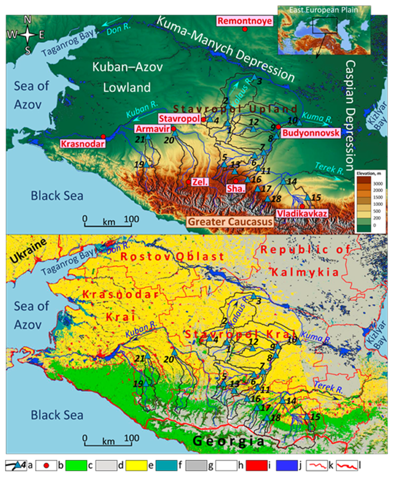
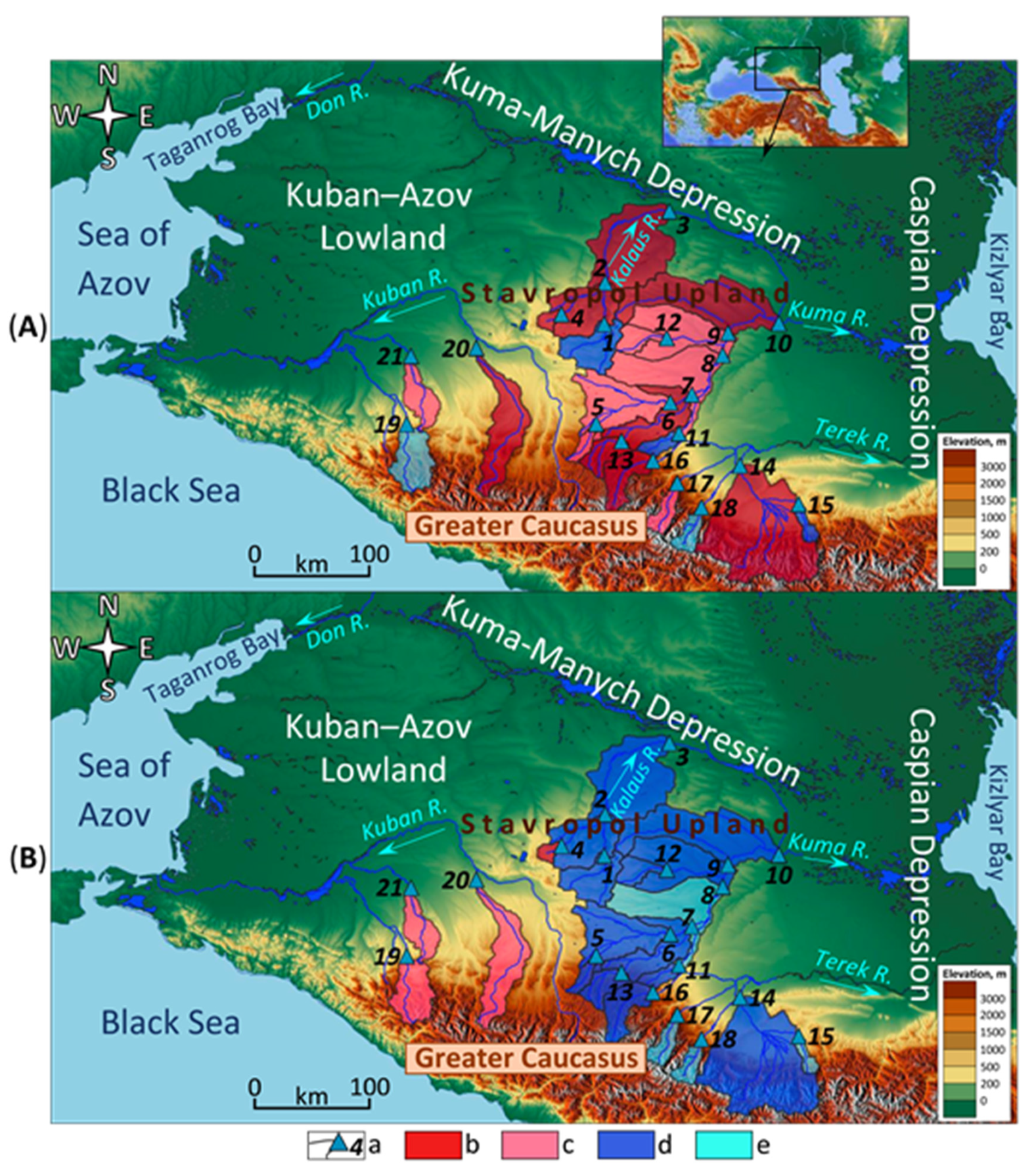
2.1. Study Area and Objects

The Stavropol Upland. The study’s principal territory is the Stavropol Upland, located in the central part of the Ciscaucasia (Figure 1). Belonging to the basins of the Sea of Azov (through the lower Don River) and the Caspian Sea, respectively, the Kalaus River and the Kuma River form the main river systems within the Stavropol Upland. Their lowest parts are situated in the tectonogenic Kumá-Mánych Depression and Caspian Depression (see Figure 1). Within the upland, absolute heights from 300 to 600 m prevail, while within the above-mentioned depressions—less than 25 m a.s.l. The basins mentioned above are divided by river valleys and relatively small dry valleys (bálka–Russ.) into plateau-like outlier massifs and ridges.
The Stavropol Upland is composed mainly of clays, sandstones, and limestones; loams (including loess-like ones) are predominant in the eastern part of the upland’s surface. The prevailing modern soils in the upland are medium-humus chernozems and low-humus ones in its western part. In the Kuma-Manych Depression and the western part of the Caspian Depression, loamy castanozems and solonetzes are most widespread [36]. The mean annual precipitation amount ranges from 400 mm in the east to 600 mm in the west of the upland and less than 300–400 mm in the lower part of the river basins. This is in marked contrast to the Greater Caucasus, where the upper “floor” (starting from an altitude of about 2000 m) is located in the area of influence of the western air transport (the impact of the Atlantic Ocean and the Mediterranean Sea). At the height of about 2000 m, the ridge’s northern slope has approximately 1500–2500 mm of annual precipitation in the western sector, while in the eastern sector—less than 1500 mm (https://bigenc.ru (accessed on 21 December 2020)).
May and June are the months with the most precipitation. On the contrary, January and February (and November in the east of the upland) are the months with the least precipitation. Winters are rather mild (−3 to −5 °C, on average); summers are comparatively warm (20 to 26 °C, on average). In the past, steppe vegetation prevailed in the river basins, and motley grasses and feather grasses (Stipa and others) were widespread there; broadleaf forests were often found in numerous small dry valleys. Natural landscapes have been plowed over a large area—up to 60–70% in the basins’ main (central) parts [36]. Due to a combination of significant dissection of the local topography, a relatively high steepness of local slopes, and relatively less fertile soils, in the sub-basin of the upper reaches of the Kalaus River (upriver of the village of Sergiyevka (Sérgiyevka), see Figure 1), the share of cultivated land is lower there: in 1985 (i.e., during the late USSR) and 2015, it was estimated at 46% and 40%, respectively [37].
The Stavropol Upland is located in the Stavropol Krai (66,160 km²; more than 2.8 million people), one of the most soil-fertile and agriculturally developed administrative regions of all Russia (see Figure 1). In 2006–2017, cultivated land occupied, on average, about 45% of the krai’s total area (see below).
The Kalaus River as a reference river. The total length of the Kalaus River (see Figure 1) is 436 km; the river’s weighted average gradient is from 1.6 to 0.7‰ and less in the lowest reaches. The altitude difference between the headwater and the mouth of the river is about 660 m. The banks of the river are relatively high and steep (Figure 2).
The Kalaus River has 81 tributaries with a total length of 936 km. The main sources of water in the river are snowmelt-induced and rainfall-induced waters. The underground component is relatively small. The hydrological regime of the Kalaus River is a regime with spring (snowmelt-induced) floods (February to March) and rainfall-induced floods in the warm season (partly March to partly November). In the summer–autumn season, it is difficult to irrigate agricultural land; in the conditions of the region’s relatively arid climate, this circumstance results in the need for artificial irrigation at the expense of adjacent territories (mainly the Kubán River basin, see Figure 1). This also applies to the Kuma River, which additionally receives water from the neighboring full-flowing Térek River. The location of main irrigation canals in the study area can be found in Supplementary Material 1.
Several decades ago, the Kalaus River belonged to the small group of rivers with the greatest turbidity (mostly sediment concentration) among all Russian rivers. This was owing to dissected local topography (this contributes to a high degree of sediment delivery to the river network), relatively erosion-poorly stable rocks (primarily loess-like loams overlapping bedrocks) composing the surface of the river basin, a high degree of plowing of soils in the basin, and also due to active deformations (mainly lateral) of the riverbeds of the Kalaus River’s hydrographic network in loamy and clay riverbanks (see Figure 2).
The modern total sediment load of the Kalaus River is almost entirely (approximately 98%) represented by its suspended sediment component [36]. Until the 1980s and possibly even the 1990s, spring (snowmelt-induced) suspended sediment load in the rivers of the basin amounted to 45–70% of the total annual load, while summer and autumn–winter sediment load did not exceed 40% and 10–15%, respectively [36]. In small rivers of the Kalaus River basin, sediment load and water discharge were (and still are) regulated by a comparatively large number of ponds formed by earthen dams in small dry valleys. This is especially true for the sub-basin of the middle reaches of the river. The ponds were created mainly during the late USSR (the 1970s and the 1980s).

2.2. Data and Their Sources

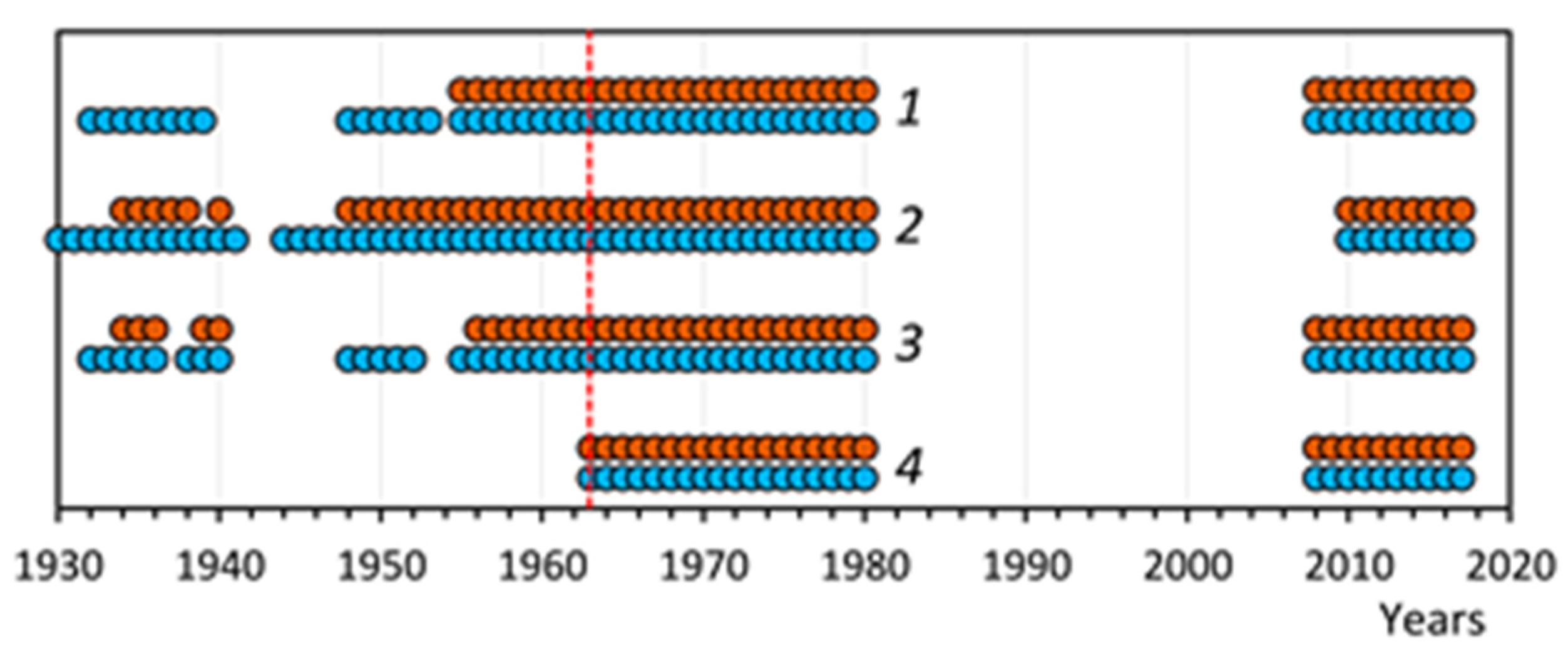
2.2.1. Hydrological Data

To assess contemporary trends in river water discharge (further–discharge) and suspended sediment load (further–load), as well as the overall intensity of erosion processes within the Stavropol Upland, the study used the results of long-term observations at 13 state hydrological (gauging) stations in the basins of two rivers—the Kalaus River and the Kuma River, which drain the prevailing area of the upland (see Figure 1; Table 1). The study’s basic (reference) materials were the results of long-term discharge/load monitoring at four hydrological stations in the Kalaus River basin (see Figure 1; Table 1). The basin’s area covered by the monitoring is 9100 km2, i.e., about 94% of the basin’s total area.
To evaluate the regionality of discharge/load-trends identified for the Stavropol Upland, available long-term series of the studied hydrological characteristics at eight additional gauging stations (sub-basins) of neighboring rivers (the Terek River and the Belaya River) of the central part of the northern slope of the Greater Caucasus were also analyzed (see Table 1; Figure 1). Thus, the total area covered by hydrological monitoring in this study is 55,554 km2.
The state monitoring results were available from hydrological collections of the former USSR [38,39,40,41,42], the Russian State Water Register (http://voda.mnr.gov.ru (accessed on 14 October 2020)), and the automated information system of state monitoring for water bodies (http://gmvo.skniivh.ru (accessed on 10 October 2020)) of the Federal Agency for Water Resources of the Ministry of Natural Resources and Environment of the Russian Federation.
The data on discharge and load in the Kalaus River basin were available for the years presented in Figure 3. Unfortunately, due to lack of available data, there were interruptions in the series of observations, the most significant of which was confined to 1981–2007/2009. The discharge data collected were summarized in the long-term series on mean annual, mean monthly, maximal, and minimal (per annum) discharge (m3 s−1) at the aforementioned hydrological stations. For the remaining 17 rivers studied, these data were limited only to mean annual values. According to [43], observations for the discharge of rivers of the former USSR and modern Russia were carried out according to a single standard program, several times daily (mainly by converting water level into discharge).
The load data collected for the Kalaus River basin were summarized in the long-term monitoring series on mean annual and maximal (per annum) suspended sediment concentration (kg m−3), as well as mean annual and mean monthly load (kg s−1) for the aforementioned hydrological stations. For all of the remaining 17 rivers studied, these data were limited only to mean annual values. According to [44], the average error in estimating the mean annual values of the load in gauging stations in the former USSR was 8–10%. It could probably have somewhat increased in the last decades.

2.2.2. Climate Data

Long-term data on monthly/annual air temperature and precipitation for two periods studied were collected and then analyzed for eight regional meteorological stations (see Figure 1). For the stations in the city of Stavropol and the city of Budyonnovsk, reliable information on long-term changes in soil temperature (March) and snow cover depth (February) were also collected and processed. All of these data were available from the All-Russia Research Institute of Hydro-Meteorological Information—World Data Center (http://meteo.ru (accessed on 14 October 2020)).

2.2.3. Land Use/Cover Data

Information on the distribution of cultivated land area within the Stavropol Krai (where the reference Kalaus River basin and the predominant part of the Kuma River basin are located) for different time intervals (during the late USSR period (1970, 1975, 1980, 1985, 1986, 1987) and the post-USSR period (annually for 1992–2017)) were collected and analyzed to semi-quantitatively estimate the probability of the anthropogenic (mainly agricultural) impact on the long-term temporal dynamics in discharge and load. The information was detailed for principal crops such as cereals, perennial, annual crops, and sunflower crops. The sources of the information are statistical collections (bulletins) of the former USSR [45,46] and also electronic statistical resources of the Russian Federation (https://fedstat.ru (accessed on 2 November 2020)).
To qualitatively assess the potential impact of the number of livestock (cattle, sheep, and goats; units per annum) on temporal changes of the above-mentioned hydrological variables, relevant information on the Stavropol Krai cumulatively for all types of farms for 1970, 1975, 1980, 1985, 1986, 1987, 1990, 1995, 2000, 2005, 2010, 2014, 2018, and 2019 were also collected and analyzed. The sources of the information are [45,46], the Big Russian Encyclopedia (https://bigenc.ru/geography/text/4162171 (accessed on 5 November 2020)).
Additionally, information on the annual number of the main types of farm machinery (tractors and grain combine harvesters) in the Stavropol Krai cumulatively for all types of farms for 1970–1975 and 2007–2019 (https://gks.ru (accessed on 5 November 2020)) were collected and processed to identify the dynamic of the “load” (units per 103 ha) of this machinery on cultivated land within the administrative region during these periods.

2.3. Methods

2.3.1. Hydrological Data Processing

Two periods were distinguished in the long-term monitoring series of both discharge and load/concentration because of differences in their characteristics and dynamics: 1963–1980 (used as a baseline period) and 2008–2017. The first period preceded the onset of active climate change and river discharge in the region (around 1980), while the second period, on the contrary, became the time of relatively more significant climatic and hydrological transformations in Eastern Europe [1,2,3,5,13,14,15,16]. On the other hand, the period from the beginning of the 1960s to 1987/1988 was marked by the highest level of agricultural development in the country [26] and, accordingly, in the study region, while 2008–2017 was a time of relative stabilization in agriculture degradation that followed the USSR’s collapse in 1991 (the 1990s and early 2000s) [9,12,21,47]. Consequently, distinguishing these two periods makes it possible to reveal contemporary discharge/load trends of the regional rivers studied against the background of simultaneously occurring changes in climate and land use/cover over the last six decades.
Along with the calculation of averaged long-term values, specific values of mean annual, maximal (per annum), and minimal (per annum) water discharge were also calculated for each distinguished monitoring period: M(WD)—integral specific discharge (L s−1 km−2) upriver of the corresponding hydrological station for the corresponding monitoring period; and ∆M(WD)—differential specific discharge (L s−1 km−2), which is calculated as follows in Equation (1):
M(WD)i = (WDiWDi+1)/(SiSi+1),
WDi (L s−1)—mean or extremal discharge of a river at a hydrological station i (with a total basin area Si (km2) upriver of this station); WDi+1 (L s−1)—mean or extremal discharge of the river at the nearest hydrological station i + 1 located upriver (with a total basin area Si+1 (km2) upriver of this station). When ∆M(WD)i > ∆M(WD)i+1, a larger runoff (discharge) is formed in the sub-basin (SiSi+1) compared to the sub-basin Si+1 located upriver. However, when ∆M(WD)i < ∆M(WD)i+1, the opposite situation is noted. This allows identifying the areas (sub-basins) of the most intense water runoff formation and its year-to-year variability in a particular river sub-basin.
Along with the calculation of averaged long-term values, specific values of mean annual suspended sediment load were also calculated for each distinguished monitoring period: SSY—integral suspended sediment yield (Mg km−2 y−1; 1 Mg = 1 ton) upriver of the corresponding hydrological station for the corresponding monitoring period; and ∆SSY—differential suspended sediment yield (Mg km−2 y−1), which is calculated as follows in Equation (2):
SSYi = (SSLiSSLi+1)/(SiSi+1),
SSLi (Mg y−1)—annual load of a river at a hydrological station i (with a total basin area Si (km2) upriver of this station); SSLi+1 (Mg y−1)—annual load of the river at the nearest hydrological station i + 1 located upriver (with a total basin area Si+1 (km2) upriver of this station). When ∆SSYi > ∆SSYi+1, a larger sediment yield is formed in the sub-basin (SiSi+1) compared to the sub-basin Si+1 located upriver; however, ∆SSYi < ∆SSYi+1, the opposite situation is noted. This allows identifying the areas (sub-basins) of the most intense sediment formation (mechanical denudation, including primarily sheet/rill/gully erosion) and its year-to-year variability in a particular river sub-basin.
Despite some methodological flaws, river sediment load/yield was/is widely used in world practice to estimate the temporal variability of erosion (more broadly—mechanical denudation) intensity in fluvial systems of various scales [21,48,49,50,51,52,53,54,55,56]. It should always be borne in mind that sediment load/yield cannot serve as an absolute measure of all erosion products due to a complex mechanism for delivering sediment from erosional areas to riverbeds. It depends on a large set of factors such as geological structure, morphometry/morphology of slopes, the density of permanent and temporary streams, basin area, climatic characteristics, features of natural landscapes, and the nature of their anthropogenic transformation, etc. [26,57,58,59,60,61,62]. This is especially important to consider when assessing the spatial heterogeneity of erosion (mechanical denudation) intensity. However, the importance and accuracy of sediment yield/load as an indicator of the temporal dynamics of erosion (mechanical denudation) in the basin increases noticeably when assessing the overall variability of the intensity of erosion within any one river basin for different time intervals (the temporal dynamics of sediment load/yield relative to one gauging station) [21].

2.3.2. Land Use/Cover Data Processing

To identify the role of agricultural activity (land cover changes) in long-term sediment-load/erosion changes, the integral (generalized) erosion resistance index—C-factor (ΣC)—was calculated for the warm (rainfall) season (April to November) during two periods (1970–1991 (the late USSR) and 2006–2017) for the whole Stavropol Krai. The index is a weighted average that considers both the area occupied by one or another crop (or agrocenosis) in the corresponding period and its individual C-index. The ΣC index was calculated only for the crops listed above as follows (Equation (3)):
ΣC = (C1 × F1 + C2 × F2 + … + Cn × Fn)/(F1 + F2 + … + Fn),
C1, C2Cn—individual C-indices for different analyzed crops (natural meadow vegetation—0.016, perennials—0.02, sunflowers—0.43, cereals—0.48, and annuals–0.48), averaged over the warm period [61]. F1, F2Fn—the average areas occupied by these crops in the corresponding period. ΣC varies from 0 to 1. The lower ΣC, the better one or other crop (or agrocenosis) protects the soil against sheet/rill erosion processes.
The changes in the “load” (τ, units per 103 ha) of farm machinery on cultivated land within the Stavropol Krai between 1970–1975 and 2007–2019 were calculated as follows in Equation (4):
τ = n/F,
n—the average annual number (units) of tractors or grain combine harvesters for the corresponding period; F—the average cultivated land area (ha) for the corresponding period: for tractors—the total area of cultivated land in the Stavropol Krai, for grain combine harvesters—only cultivated land area under grain crops.

2.3.3. Statistical Processing

To identify statistically significant differences in all averaged values of the studied hydrological and other characteristics between the aforementioned monitoring periods, the Student’s t-test was used. All of the averaged values were calculated with a 95% confidence interval.

3. Results

3.1. Contemporary Hydrological Changes in the Kalaus River Basin

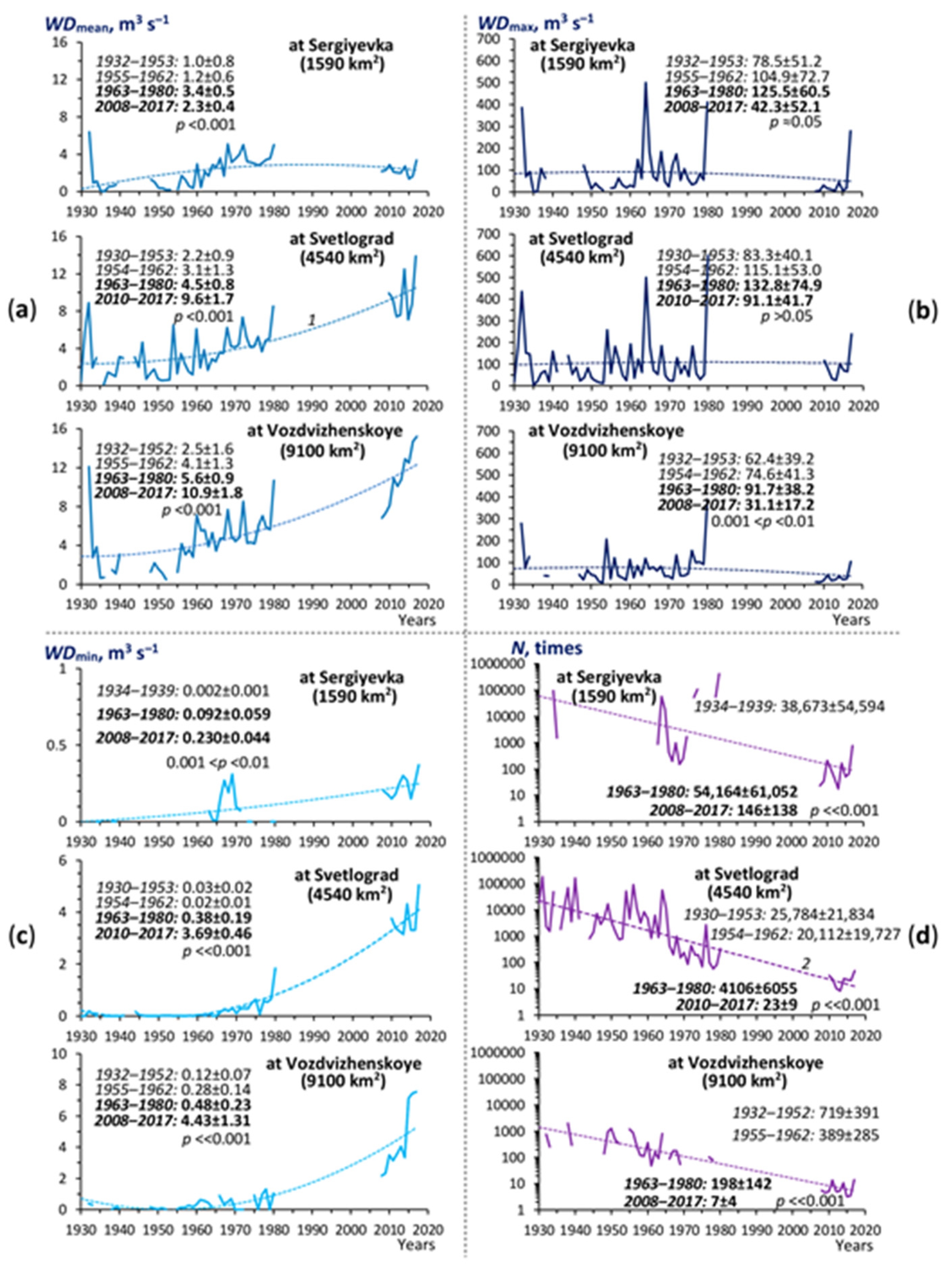
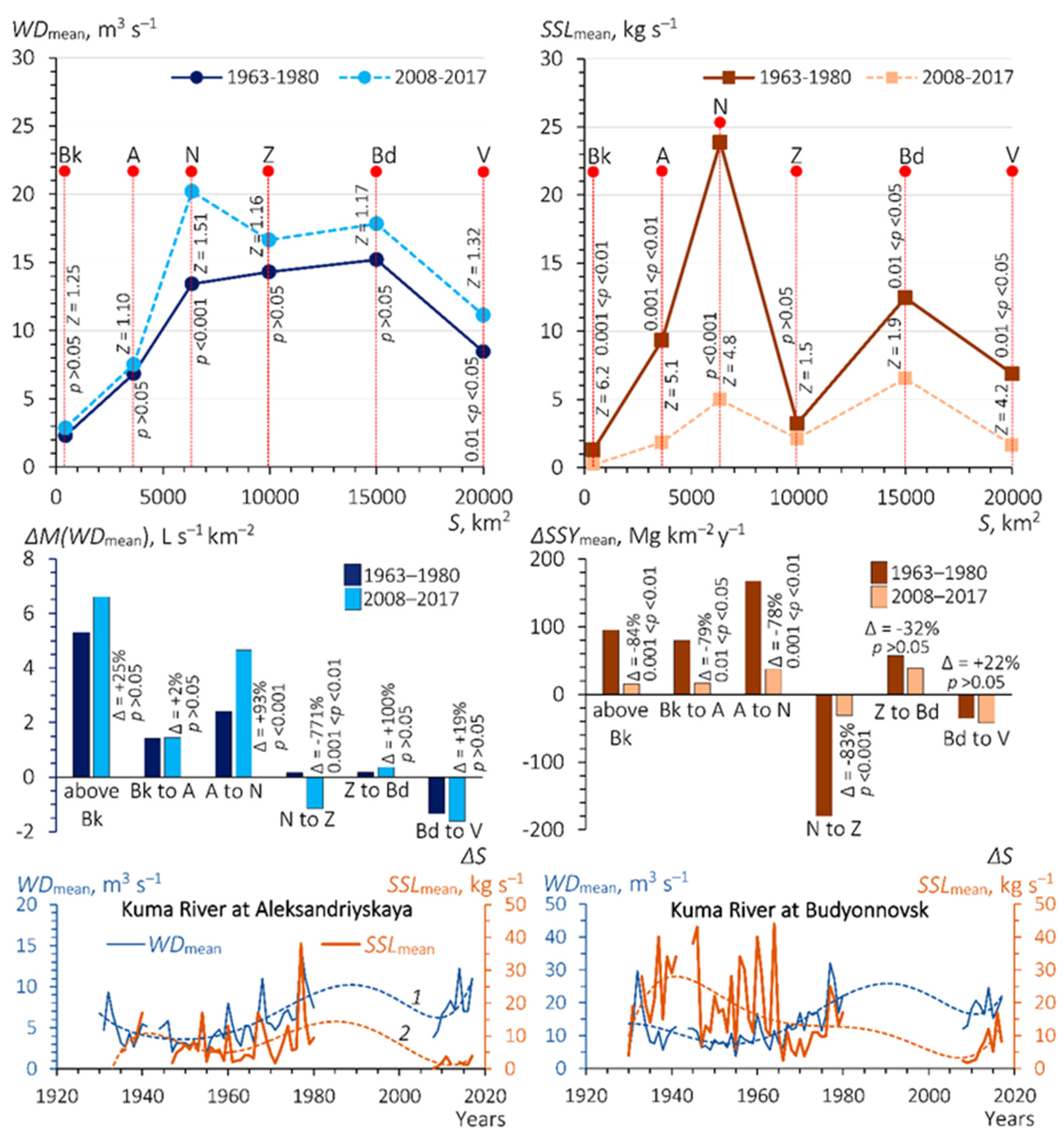
3.1.1. Long-Term Trends in Water Discharge

Analysis of the available data on the long-term water discharge dynamics at all three hydrological stations along the Kalaus River allowed drawing the following findings (Figure 4).
From the 1930s–1940s to the 2000s–2010s, there has been a steady upward trend in the discharge of the Kalaus River in most of its basin. The mean annual discharge in 2008/2010–2017 increased by about two times compared to 1963–1980, and 4.4 times compared to 1930/1932–1952/1953 in the middle and lower reaches of the river (see Figure 4a). However, in the river’s upper reaches, the discharge was even lower in the recent decades than in 1963–1980. The noted trend was mainly due to an increase in the baseflow (base discharge), which was expressed, for example, by a significant rise in minimal water discharge of the river, especially in its middle and lower reaches: between 1963–1980 and 2008/2010–2017, the minimal (per annum) water discharge increased there by 9.2–9.7 times, while in the upper reaches of the river, only by 2.5 times (see Figure 4c). On the other hand, maximal (per annum) water discharge in the river in 1963–1980 also had a general tendency to increase (by 47–60% compared to 1930/1932–1953), which, after the 1980s, was most likely replaced by the opposite trend (a decrease by 31–66% between 1963–1980 and 2008/2010–2017) (see Figure 4b).
The aforementioned long-term discharge dynamics resulted in a significant reduction in its intra-annual variability or amplitude (N, the difference between maximal and minimal discharge per annum) in the Kalaus River over the past decade compared to 1963–1980. This reduction was substantial in the river’s middle and upper reaches (see Figure 4d).
Based on the temporal dynamics of differential specific water discharge (see Equation (1)), the sub-basin of the upper reaches of the Kalaus River turned out to be the territory with the greatest contribution to the formation of maximal discharge during the entire analyzed time (Figure 5b). It is noteworthy that in this part of the river basin, there have been significant reduction in the maximal discharge between 1963–1980 and 2008/2010–2017.
The differential specific minimal discharge (see Equation (1)) of the Kalaus River did not change much between the analyzed hydrological stations in 1963–1980, increasing slightly in the sub-basin of the middle reaches. Over the last decades, the situation has changed dramatically due to a sharp increase in the minimum discharge, especially in the river’s middle and lower reaches (see Figure 5c).

3.1.2. Long-Term Trends in Suspended Sediment Load/Concentration

Analysis of the available data on the long-term dynamics of sediment load/concentration at all three hydrological stations along the Kalaus River allowed drawing the following findings:
Since the 1930s–1940s (at least), there has been a steady general upward trend in sediment load/concentration of the Kalaus River, which lasted until the beginning of the 1980s (or maybe later). Moreover, the trend in suspended sediment load was more essential (Figure 6).
Herewith, the sharpest increase in the content of suspended sediment in river waters occurred after 1968: during 1968–1980, a concentration of suspended sediment particles with a value of more than 1000 g m−3 was observed during, on average, about 75% of the annual time, while a concentration of more than 5000 (but less than 50,000) g m−3—about 41%. For comparison, during 1948–1967, these values were only 14% and 4.4%, respectively (Supplementary Material 2). Due to the period 1968–1980 (the mid-1990s?), the Kalaus River was considered one of Russia’s most sediment-reach rivers. After the late 1980s (the mid-1990s?), sediment load/concentration began to reduce at all three analyzed hydrological stations along the Kalaus River (see Figure 6).
When analyzing the temporal dynamic of sediment load, it is important to consider its changes relative to discharge in river basins to minimize surface water runoff’s role when analyzing the causes of temporal variability in the load formation. Figure 7 shows a more or less clear differentiation of groups of years with a various mean annual load of the Kalaus River relative to the mean annual discharge of the river in these years. The years of the relatively active (enhanced) forming the load of sediment in the river’s basin are comparatively compactly grouped in the time interval from 1960 to 1980. This indicates that, other things being equal, at the same mean annual water discharge, the increased mean annual load of sediment during this period could be due to external (mainly anthropogenic) factors. On the contrary, the relatively weak formation of sediment load in the river basin was dated to 2008–2017, despite the rather large range of discharge changes along the river during these years (see Figure 7).
The most significant decrease (Z) in sediment load/concentration of the Kalaus River between 1963–1980 and 2008/2010–2017 occurred in the upper reaches of the river (by 6.6–12.5 times), the smallest–in its middle and lower reaches (by 3.3–6.0 times) (Figure 8a). During 1963–1980, the integral suspended sediment yield tended to decrease regularly downriver. In 2008/2010–2017, this tendency was replaced by the one in which the largest integral suspended sediment yield was observed in the middle reaches of the river, the smallest–in the upper reaches (see Figure 8b,c).
To correctly analyze the effect of changing environmental conditions within the river basin’s surface on sediment load/concentration, it is important to evaluate the spatiotemporal changes in the differential suspended sediment yield [57]. The largest relative and absolute decrease in this yield between 1963–1980 and 2008/2010–2017 occurred in the sub-basin of the upper reaches of the Kalaus River (upriver of Sergiyevka—by 12.5 times); the smallest (and statistically insignificant)—in the sub-basin of the middle reaches of the river, between Sergiyevka and Svetlograd—by 1.5 times (see Figure 8e). It follows from these facts that the sub-basin of the upper reaches of the Kalaus River during 2008/2010–2017 ceased to be the predominant source of suspended sediment formation in the entire river basin compared to 1963–1980 when this sub-basin exceeded the sub-basin of the middle reaches by the intensity of river sediment formation by 3.4 times, and the sub-basin of the lower reaches—by 15.5 times. The sub-basin of the contingently lower reaches of the Kalaus River, located between Svetlograd and Vozdvizhenskoe (about 50% of the entire studied part of the river basin), reduced its role as a source of sediment in the river by more than half in 2008/2010–2017 compared to 1963–1980 (see Figure 8d,e). Thus, the main territory of river sediment formation in the Kalaus River basin in 2008/2010–2017 became the sub-basin of the river’s middle reaches, which is currently more than twice active concerning sheet/rill/gully erosion and sediment formation than the sub-basin of the upper reaches of the river. The proportion of transit suspended sediment in the lower and especially in the middle reaches of the river decreased between the indicated periods (Figure 8f). Consequently, the middle sub-basin of the Kalaus River should become the arena of the most active erosion-control measures and sediment interception measures in the present and the future.
There was a generally steady temporal shift tendency in maximal (per annum) mean monthly water discharge and suspended sediment load in the Kalaus River from early spring to early summer since the 1930s. In the 1930s–1950s, these maximums were observed, on average, in March, whereas in 2010–2017—in June (Figure 9). Despite several abnormal years (1950, 1953, 1965, 1971, 1973, 1977, 1978, 2012, and 2013), when discrepancies between these maximal mean monthly water discharge and sediment load were recorded (see Figure 9c), these changes in discharge/load were observed in the same month in the majority of cases. An explanation of the highlighted anomalies is given in Supplementary Material 3.

3.2. Contemporary Hydrological Changes in the Basins of Kuma River and the Additionally Studied Rivers of the North Caucasus Region

Throughout the studied length of the Kuma River, as well as in its tributaries, there were steady and statistically significant in the overwhelming majority of cases downward trends in mean annual SSL between 1963–1980 and 2008–2017, despite the regular increase (statistically insignificant in most cases) in mean annual discharge in this river basin (Figure 10; Table 2). Especially essential reduction in sediment load/yield occurred in the highest parts of the Kuma River basin, i.e., the lower part of the Greater Caucasus’s northern slope and on the Stavropol Upland (the Tomuzlovka River basin). Downriver, these changes were less significant.
There were unidirectional discharge trends between the two analyzed periods in the Terek River’s upper reaches (see Table 2; Figure 1). However, in sediment load/yield, its decrease trends were traced in all rivers of this basin, but they were statistically insignificant (see Table 2).
No unidirectional and statistically significant discharge trends were revealed between 1963–1980 and 2008–2017 for the three studied rivers’ basins in the western part of the Greater Caucasus’s northern slope (see Figure 1). However, the changes in load/yield were expressed in upward trends in all of these basins, but they were also statistically insignificant (see Table 2).

3.3. General Patterns of Contemporary Trend Changes in Discharge/Load of the North Caucasus Region’s Studied Rivers

Figure 11 cartographically summarizes all of the above information on the distribution of contemporary trends in mean annual water discharge and suspended sediment load in all 21 studied river basins of the region, taking into account their statistical significance. The general prevailing tendency to increase in the last more than half a century is clearly visible in water discharge. In contrast, the suspended sediment load showed a predominant tendency to decrease in the analyzed rivers. Moreover, the following relatively clear pattern was observed: all studied rivers flowing east of the submeridian upper reaches of the Kuban River tended to decrease the sediment load in the specified period, while rivers flowing westward, but within the northern slope of the Greater Caucasus, tended to increase suspended sediment (a statistically insignificant increase).

4. Discussion

Considering the study region’s physical geographic conditions, the leading causes of the above-mentioned long-term changes in discharge and load of the Kalaus River and Kuma River basins could be, in our opinion, changes in climate and land use/cover. We exclude any significant role of the processes associated directly with the Earth’s internal energy (mainly tectonic movements) in the indicated dynamics.

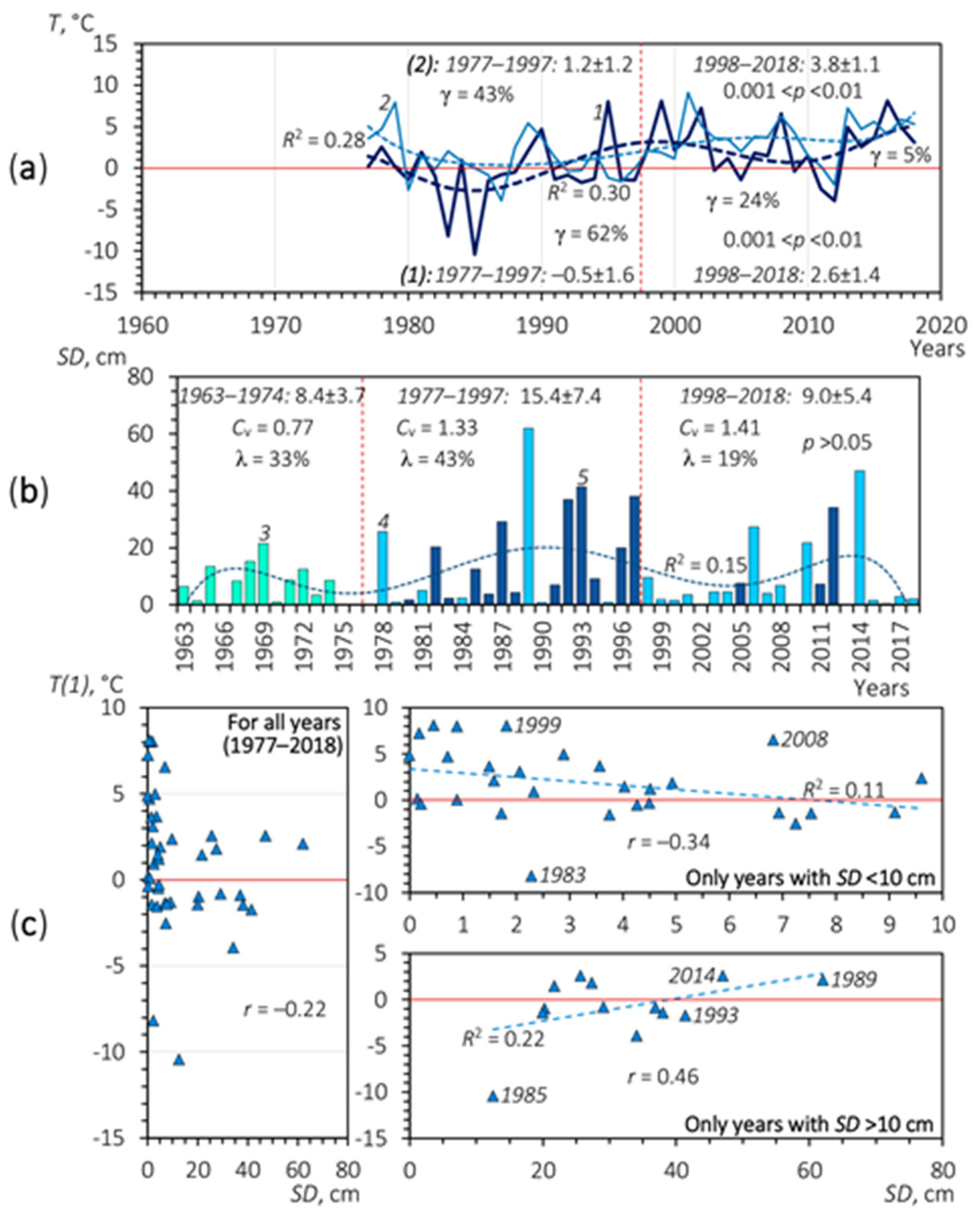
4.1. The Impact of Climate and Climate-Induced Changes

The collected and processed data on climate change in the region under study, based on long-term air temperature/precipitation observations at two meteorological stations closest to the Kalaus River and Kuma River basins, are summarized in Table 3.
Following these data, it was possible to reveal the influence of modern climate change on discharge and load/yield of the rivers (on the example of the Kalaus River) during the main seasons of their formation—the spring snowmelt period (snowmelt-induced flood, mostly March) and the warm (rainy) season (partly March to November).

4.1.1. Changes in Surface Water/Sediment Runoff Formation during Snow Melting

In the relatively cool/cold months in the region (November to March), only in March, there was a statistically significant rise in air temperature (see Table 3). This trend was accompanied by a statistically significant increase in rainfall this month, sometimes in the snowfall form.
A distinctive feature of both this region and Russia´s vast expanses outside it is that the snow, falling during the winter months, accumulates there in the form of snow cover, except for evaporation losses. With the advent of spring, the cover melts, forming a surface runoff and carrying out the soil erosion destruction primarily where there are favorable environmental conditions for this (mainly within arable land). Figure 12 demonstrates the combined diagrams of temporal dynamics of temperature on the soil (to a depth of not more than 10 cm from the surface) in March and the depth of snow cover in February, which are derivatives of the changes mentioned above. We have purposefully identified the two first 10-day periods in March in terms of soil temperature. In Russia’s southern regions, snowmelt processes occur comparatively quickly, not dragging on as long as, for example, in the East European Plain’s forest zone for a month or more. Consequently, it is essential to show when the processes of formation and temporary changes in the snowmelt runoff and erosion processes caused by it are the most active.
Since the late 1980s, according to data from the Stavropol’s meteorological station, a steady tendency towards an increase in the temperature of the topsoil was found, especially in the first half of March (with a sufficiently high statistical significance), when snow melting is usually observed in the upland (see Figure 12a). After 1997, the topsoil’s negative temperatures at the beginning of March became more an exception than the rule that dominated until the mid-1980s (including, most likely, the 1950s–1970s). Due primarily to an increase in air temperatures in March, this trend was also partially determined by snow cover depth changes. This was especially well-manifested when comparing two periods: 1977–1997 and 1998–2018 (see Figure 12b). The snow cover’s warming effect on the soil was comparatively effective, primarily with snow depths more than 10 cm (the direct and relatively close relationship between snow depths and soil surface temperatures). An inverse relationship was observed between these characteristics (see Figure 12c) with snow depths of less than 10 cm. It indicates, most likely, the essential role of the thermal air balance in forming the thermal balance of the topsoil in the absence of a relatively deep snow cover. The smaller this depth (<5 cm), the stronger the influence of the thermal balance of air (direct solar radiation is also possible) on temperatures of the topsoil, which determine the depth of its freezing before and during the snow-melting time.
In the context of our study, the most important is the resultant of all of these changes—a change in the conditions of formation of water runoff and sediment load/yield in the studied rivers of Ciscaucasia. According to the Barabanov’s rule [63,64], formulated based on long-term observations at experimental runoff plots in the steppe and forest-steppe zones of European Russia, at a certain minimum value of one of the three limiting factors (water reserves in the snow, soil freezing depth, and soil moisture), no surface water runoff is formed regardless of the indicators of other factors. If the soil is frozen to ≤50 cm deep (the farther south, the less this critical level), then there is no surface runoff regardless of its moisture and water reserves in the snow. The bulk of the meltwater is filtered into the soil and then into underlying rocks, replenishing groundwater volumes. The effect of the depth of soil freezing on surface runoff is also confirmed by modeling and field experiments [65,66,67,68].
Unfortunately, we did not have data on the depth of soil freezing over the last several decades in the region. Still, there is a direct and close correlation (ceteris paribus) between this value and the topsoil’s temperature [63,64,69,70,71]. Hence, we had reason to restore (at least at a qualitative level) the probability of surface runoff and its long-term dynamic over the past few decades. As shown in Figure 12b, the active formation of snowmelt-induced surface water runoff could potentially be in 1977–1997: of 21 years of this period, 13 years (62%) could well have this runoff during the first half of March. This runoff could carry out active erosion work and, therefore, sediment formation.
It can also be assumed with high probability that even before the 1980s, the conditions for the formation of snowmelt runoff and snowmelt-induced sheet/rill/gully erosion in the Kalaus River basin and most of the Kuma River basin differed little or were even more favorable than in the 1980s–1990s. We do not have direct data on soil temperature to verify our findings. Nonetheless, the fact that winters (especially in January and February) in the 1960s–1980 were more severe than since the 2000s (see Table 3) is an essential indirect argument in favor of these findings, taking into account the Barabanov’s rule noted. Moreover, a smaller amount of precipitation (the depth of snow cover), especially in January (see Table 3), could also contribute to more significant soil freezing in the 1960s–1980.
The following period, 1998–2018, was contrasted concerning the period 1977–1997. Snowmelt runoff and erosion processes in the Kalaus River basin, taking part in the river’s sediment load formation, could be observed only during three years (14%) in 1998–2018. In most years, there was an active transformation of spring surface meltwater into soil/subsoil (mainly groundwater) runoff during this period. The consequence of this was a previously marked reduction in maximal water discharge (in the river’s upper reaches, see Figure 4a and Figure 5b), maximal and mean annual concentration of suspended sediment, and the load (annual values) of suspended sediment of the Kalaus River and the Kuma River (see Figure 6, Figure 8 and Figure 10) in the last decades.
As for climate monitoring data on the eastern part of the Stavropol Upland, the climatic trends noted above were also stored there in the last decades, according to the Budyonnovsk’s meteorological station. The following temporal dynamics were found there: in temperatures on the surface of the soil (the second 10-day period of March): 1977–1997: 0.96 ± 1.61 °C, 1998–2018: 3.81 ± 1.48 °C (0.01 < p < 0.05); in depths of the snow: 1938–1973: 7.1 ± 3.3 cm, 1977–1997: 4.6 ± 2.2 cm, 1998–2018: 3.6 ± 3.4 cm (for all periods p > 0.05). These data on Budyonnovsk can also be considered quite representative for the Kuma River´s entire basin (see Figure 1), at least for its larger, plain part.

4.1.2. Changes in Surface Water/Sediment Runoff Formation during the Warm (Rainy) Season

Table 4 summarizes the inter-period dynamics of precipitation with different depths in all seasons since 1966 for two meteorological stations in Stavropol and Budyonnovsk. Despite a general decrease in the number of rains (and snowfalls) with a small precipitation depth (≤10 mm) in the last three decades compared with 1966–1980, there was an increase in precipitation with a depth of >20–30 mm. These precipitation depths can create surface water runoff that can erode the soil and form sediment. An increase in heavy rainfall (in the warm season) is a general trend that was observed almost throughout the southern half of the East European Plain and the Ciscaucasia with global warming. It was proved that the frequency and intensity of heavy rains in Russia as a whole had risen sharply over the past half-century, increasing by 1–2% every ten years [72]. It is likely that the noted dynamic could result in a slight increase in the intensity of soil erosion predominantly on cultivated land of the Stavropol Upland in the warm season and therefore increase the load of suspended sediment in the Kalaus River and Kuma River networks. However, it should be kept in mind that all heavy rains (with a depth of more than 30 mm) occur in the region during the warm season (see Table 4) when cultivated land is comparatively well protected by either crops or stover, which also protects the soil against both water erosion and wind erosion. Therefore, not every heavy rain and not everywhere (depending on sowing crops) could cause proportionally enhanced soil erosion.
The temporal shift in the month with the largest discharge and load in the Kalaus River from the beginning of spring (March) to the beginning of summer (June) during the last 80 years (especially since the 1970s), noted earlier in Figure 9, can be explained, on the one hand, by the weakening of surface water runoff caused by snow melting due to warming at the end of the cold season. On the other hand, it could be owing to a relative increase in rainfall-induced runoff in the warm season.

4.2. The Impact of Human Activities Changes

4.2.1. River Water Transfer

The increase in minimal and mean annual water discharge of the Kalaus River and the Kuma River (the middle and lower reaches of the rivers), noted above in Figure 4 and Figure 10, was due to the transfer of water from the neighboring more full-flowing rivers of the region (the Kuban River and Terek River) through the system of irrigation canals, which began to function since the 1960s–1970s (see Supplementary Material 1). For example, the Pravoyegorlykskiy (Right Yegorlyk) Canal, as the principal object of the Yegorlyk irrigation system, which has been operating since the mid-1970s, has an average water discharge into the Kalaus River of about 4–5 m3 s−1. This roughly corresponds to the magnitude of the increase in the minimum discharge of the Kalaus River between the periods studied. Here we would like to pay attention to the previously noted decrease in the dependence of sediment load on temporal discharge changes for 2008–2017 in the middle and lower reaches (see Figure 7b,c) of the river compared to its upper reaches (see Figure 7a). The main reason for this, in our opinion, is the aforementioned transfer of water from the basins of neighboring rivers. This water entering the Kalaus River through canals is not dynamically related to sediments coming from the river catchment due to soil/gully erosion, except for those that have formed as a result of riverbed deformations.
Unfortunately, we do not have quantitative data on the volumes of water discharged from the canals directly into the studied rivers, since significant volumes of this water were/are spent on irrigation before reaching the river network. This issue requires further study.

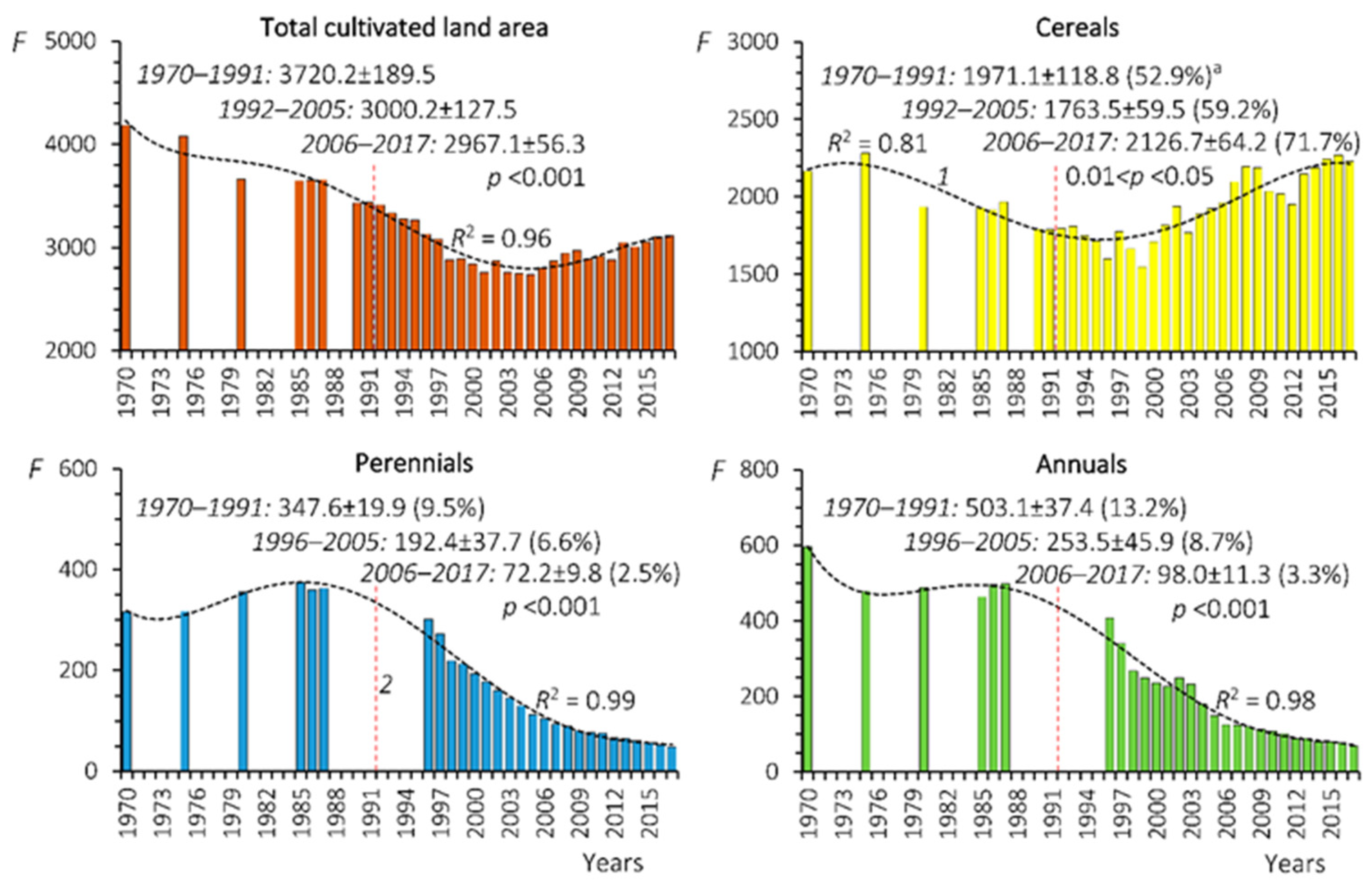
4.2.2. Cultivated Land Area Changes Impact

After the collapse of the Soviet Union in 1991/1992, agricultural degradation took place in Russia and neighboring countries of Eastern Europe, manifested, among other things, by a significant reduction in the total cultivated land area [10,11,12,17,21,73]. This degradation also affected, albeit with less intensity, the Stavropol Krai. The total area of cultivated land in this administrative region of Russia decreased by 20% from 1970–1991 to 2006–2017 (Figure 13).
The reduction in the area of cultivated land was accompanied by a change in the structure of crops: a slight increase in the area of grain crops (cereals) and a significant reduction in areas of perennial—clover, alfalfa, etc. (by 79%) and annual (by 80%) crops. Regarding perennial crops’ anti-erosion properties, it should be noted that they sufficiently reliably protect the soil against erosion due to their dense root system and significant projective cover. For instance, the washing-out of soil material under perennial grasses was on average about 50 times less than on cultivated land, according to the earlier studies by I.A. Kuznik in 1961 [74] in the forest-steppe of the Trans-Volga region of European Russia.
The sown area under sunflower increased significantly (almost by 54%, p < 0.001) between 1970–1987 and 2010–2015 in the krai, from 170.1 ± 28.0 × 10³ ha to 262.4 ± 15.3 × 10³ ha [46]. However, it is important to clarify that the main sunflower sown area is currently located chiefly in the western part of the Stavropol Krai [47], west of the main studied river basins of the Stavropol Upland.
This temporal dynamic gives a clear idea of the general change in the Stavropol Krai’s sowing fund because all of these crops together occupied (and still occupy) the predominant area in the region (in 1977–1991: 80.2%; in 2006–2017: 86.3%). In general terms, it was also characteristic of the Kalaus River basin, which occupies about 15% of the administrative region’s total area. However, in some parts of this basin, agricultural degradation could be varied. Due to the noted reduction in cultivated land area, abandoned land area that is now overgrown with natural meadow-steppe vegetation, which reliably protects the soil against all types of erosion, has increased.
The integral (generalized) erosion resistance index—C-factor (see Equation (3))—decreased insignificantly between the indicated periods (−4.8%), from 0.42 to 0.40, despite a noticeable decrease in the total area of cultivated land. This is explained by the fact that on cultivated land remained after the reduction, the C-factor, on the contrary, slightly increased (9.5%), from 0.42 to 0.46, due primarily to the expansion of cereals and sunflower crops, characterized by an average level of erosion resistance. From the data obtained, it might be concluded that the dynamic of crop areas, expressed through changes in the C-factor, can be one of the causes of the previously noted sediment load changes in the Kalaus River and the Kuma River. However, its overall effect was most likely not decisive. It is also likely that this influence was much more essential in some sub-basins and small catchments of the Kalaus River and Kuma River basins.
Despite a slight increase in erosion potential on the remaining cultivated land area in the recent decades (growth of the C-factor), it could be partially compensated by reducing the “load” (pressure) of agricultural machinery on plowed soils. The number of the machinery has been steadily (and very significantly) declining in Russia over the past decades after the USSR collapse [75]. However, this decrease in the Stavropol Krai (Table 5) was not so sharp compared to the rest country. Apparently, this circumstance reduced the topsoil’s compaction, thereby improving its filtration properties and, consequently, increased its erosion resistance relative to the increased heavy rains, as was mentioned earlier. Information on the mechanism of the impact of agricultural machinery on chernozems can be found, for example, in [76].
It should be noted that in the neighboring agriculturally developed administrative region of Russia, in the Krasnodar Krai, located between the Stavropol Upland and the Black Sea and the Sea of Azov (see Figure 1), a similar tendency in plowland area changes was also observed: this area reduced by almost 15% from 1970–1987 and 1996–2017.
At the same time, the intensity of sheet/rill/gully erosion and load/yield rates could also increase, even compared to the late USSR, near large settlements (cities) of the region studied, where active urbanization processes have taken place in the recent decades. For instance, this case was observed near the city of Stavropol in the Ula River basin. This river’s mean annual load increased by 1.7 times between 1963–1980 and 2008–2017 (Supplementary Material 4). The influence of urbanization and suburban economy on the long-term dynamics of discharge and load/yield requires a separate thorough study.

4.2.3. Livestock Changes Impact

There was a significant reduction in the number of livestock (cattle, goats, and sheep) (Figure 14) within old pastures that existed since the time of the late USSR, and new ones formed after abandoning cultivated land in the last decades. A significant decrease in livestock numbers on pastures after the USSR collapse was also noted almost everywhere in the Greater Caucasus’s northern slope [75]. Most likely, this resulted in a proportional decrease in the impact on soils of the region through a decrease in the topsoil compaction during trampling [77,78,79] and an increase in the biomass of meadow grassy associations. These associations increase the erosion resistance of the soil. The indicated temporal dynamics were generally correlated well with the dynamics of sediment load changes in the Kalaus River (see Figure 6 and Figure 8) and the Kuma River (see Figure 10).
Under these conditions, it was quite natural, not only the reducing of the intensity of erosion and associated sediment load/yield in various parts of the fluvial network (as confirmed by the temporal dynamics of sediment load of the rivers, noted earlier) but the gradual stabilization of erosion landforms created previously (most likely in the 1950s–1990s); for example, ephemeral and typical gullies (see Figure 14).

4.3. Neighboring River Basins of the North Caucasus Region

Based on the results from Table 2, we assume that similar trends in load/yield have occurred in the recent decades in the central part of the Ciscaucasia—to the east of the dividing line between the basins of the Kuma River and Kuban River (see Figure 1 and Figure 11). These trends were more statistically significant for plain river basins (the Kuma River basin) than for piedmont/low-mountain ones (see Figure 11).
In the western part of the Greater Caucasus’s northern slope with wetter (more forested) landscapes (see Table 1; Figure 1), the opposite tendency (but statistically insignificant) toward an increase in sediment load/yield in local rivers has been observed in the last decades (see Table 2). A commensurate rise in mechanical denudation rates in the western part of the Greater Caucasus was also indicated by [80] based on sedimentation rates in two small lakes in this region from the 1960s to the present.
Therefore, the aforementioned (by the example of the Kalaus River) combined effect of climate and land use/cover changes on reducing sediment load manifested most effectively in the lowland (plain) part of the Ciscaucasia, possibly including the lowland part of the Kuban River basin (we did not have reliable data on river sediment load). This reduction in sediment load also took place in the central part of the Greater Caucasus’s northern slope, where the overall (natural-anthropogenic) rates of mechanical denudation are generally high [81]. It was in these parts of the Ciscaucasia and the northern slope of the Greater Caucasus (its central part) that the decrease in river sediment load/yield occurred primarily due to a general reduction in the rate of sheet/rill/gully erosion in interfluves of the river basins studied. In particular, this could result from a decrease in mudflows’ contribution to river sediment load formation. They were (and still are) considered the most active precisely in the center and the east of the Greater Caucasus [82].
As for the western part of the northern slope of the Greater Caucasus and its foot (approximately west of the dividing line between the basins of the Kuma River and Kuban River), climate warming could have an essential influence on the long-term upward trend of sediment load in local river basins where the rates of natural-anthropogenic mechanical denudation are relatively generally low [81]. This is largely due to the good preservation of forests in large areas in these basins (see Figure 1, Table 1), preventing mechanical denudation. In conditions of statistically significant regional warming and statistically insignificant increase in precipitation (especially in the cold season) (Supplementary Material 5), the influence of the forestland (its relative area) on long-term dynamics could be decisive. In the well-forested landscapes, this can intensify lateral channel erosion (natural riverbed deformations) due to increased discharge and therefore increase its products in riverine waters. According to our preliminary calculations, the relationship between the forestland area in river basins and the growth rates of load/yield in the recent decades was very close for this part of the study region: the linear correlation coefficient was 0.98, according to the three studied rivers (the Belaya, Urup, and Fars rivers).

4.4. Comparison with Neighboring Regions of Europe

Finally, mention should be made that the above-mentioned hydrological (a reduction in spring snowmelt-induced discharge) and sheet/rill/gully erosion intensity changes (a decrease in annual river load/yield) in the basins of the main studied plain rivers of the Ciscaucasia (the Kalaus River and the Kuma River), in river basins of the central part of the northern slope of the Greater Caucasus (the upper Terek River basin) and possibly the lowland part of the Kuban River basin, were similar in their common features to those previously described in many regions of the neighboring East European Plain [13,14,15,16,17,19,20,21,23,25,27,28,29,71,73,83,84], in the Baltic countries (Estonia, Latvia, and Lithuania) [85], as well as in Eastern Scandinavia [86], Poland, Belarus, and in the north of Ukraine [87]. That is, it was a sizeable regional phenomenon for Eastern and Central Europe.
The revealed modern tendencies towards a decrease in sediment load in most of the North Caucasus region’s rivers correspond well with the general global tendency to decrease in the large rivers’ sediment load [88].

5. Conclusions

Based on the work made, we have come to the following key conclusions:
(i) From the 1960s to the last decades, there was a steady (but not always statistically significant) tendency to increase mean annual water discharge in the Ciscaucasia’s rivers studied. The tendency was accompanied by a substantial reduction in discharge’s intra-annual variability (N) in the rivers, especially in their upper reaches. These changes were chiefly caused by an increase in the discharge (mainly baseflow) in the warm season due to water transfer through irrigation canal systems from the neighboring river basins, characterized by much larger runoff (the Kuban River basin and the Terek River basin). The baseflow increase could be partly due to the redistribution of the spring snowmelt-induced surface runoff to the underground runoff under regional/global warming. The intra-annual variability reduction in the discharge was partly due to a decrease in maximal water discharge, which for the last at least 90 years have a maximal average level in the 1930s–1970s. The most significant reduction in water discharge in the last decades was recorded in sub-basins of the upper reaches of the rivers that drain the Stavropol Upland (e.g., the upper reaches of the Kalaus River). As for the studied rivers’ discharge of the Greater Caucasus’s northern slope, multidirectional and statistically differently significant trends in its changes were revealed there over the past decades.
(ii) There has been a predominant tendency to reduce suspended sediment load in river basins over the past more than half a century in the North Caucasus region. The most significant decreases were noted within the Stavropol Upland between 1963–1980 and 2008–2010: in the Kalaus River basin—from 70 to 92%, in the Kuma River basin—from 47 to 94%. In other words, such an essential decrease in sediment load/yield took place exactly where there were some of the sediment-richest rivers in all of Russia flowed in the middle of the 20th century. A moderate decrease in sediment load/yield was found in some river basins of the central part of the Greater Caucasus’s northern slope (17 to 94%). Statistically insignificant tendencies of an increase in suspended sediment load/yield between the periods under consideration were revealed in the river basins in the west of the Greater Caucasus. The greatest suspended sediment reduction rates were found in the sub-basins of the Ciscaucasia’s studied rivers’ upper reaches. These rivers’ sub-basins are characterized by the highest average altitude, a high degree of relief dissection, a relatively more humid climate, and comparatively more severe winters. All of the noted main changes in river load/yield were directly related to a decrease in the intensity of mechanical denudation processes (mainly sheet/rill/gully erosion processes) within these river basins due to joint changes in climate (reducing the depth of soil freezing and reducing the runoff of meltwater on it) and land use/cover (reducing cultivated land area and agricultural machinery “load” (pressure) on it, reducing livestock on pastures, etc.).

Supplementary Materials

The following are available online at https://0-www-mdpi-com.brum.beds.ac.uk/2306-5338/8/1/28/s1, Figure S1: The layout of the main irrigation canals (irrigation systems) in the study region (Supplementary Material 1); Figure S2: Inter-period changes in the number of days (per annum) with different suspended sediment concentrations recorded at the Kalaus River near the town of Svetlograd (Supplementary Material 2); Text Material S3: The highlighted anomalies … (Supplementary Material 3); Figure S4: Changes in water discharge and suspended sediment load of the Ula River, a left tributary of the Kalaus River, at the village of Staromarievka (the Stavropol Krai, SW Russia) between 1963–1980 and 2008–2017 (Supplementary Material 4); Table S5: Changes in air temperature and precipitation at some meteorological stations in the North Caucasus region between 1963(1966)–1980 and 2008–2017 (Supplementary Material 5).

Author Contributions

Conceptualization, A.V.G.; methodology, A.V.G.; software, A.V.G., A.G.S.; validation, A.V.G. and A.G.S.; formal analysis, A.V.G., A.G.S.; investigation, A.V.G., A.G.S., and M.A.K.; resources, A.V.G. and A.G.S.; data curation, A.V.G.; writing—original draft preparation, A.V.G., A.G.S., and M.A.K.; writing—review and editing, A.V.G.; visualization, A.V.G. and A.G.S.; supervision, A.V.G.; project administration, A.V.G.; funding acquisition, A.V.G. All authors have read and agreed to the published version of the manuscript.

Funding

The study was performed according to the Russian Government Program of Competitive Growth of Kazan Federal University and carried out within the framework of the intra-university grant of the Belgorod State University to support the creation and development of scientific departments—centers of excellence.

Acknowledgments

The authors thank the anonymous reviewers, Arun Mondal, the Special Issue’s guest editor, and Tammo Steenhuis, an associate editor of Hydrology, who comprehensively contributed to the manuscript by providing valuable reviews.

Conflicts of Interest

The authors declare no conflict of interest. The funders had no role in the study’s design; in the collection, analyses, or interpretation of data; in the writing of the manuscript, or in the decision to publish the results.

References

  1. Shmakin, A.B.; Popova, V.V. Dynamics of climate extremes in Northern Eurasia in the late 20th century. Izv. Atmos. Ocean Phys. 2006, 42, 138–147. [Google Scholar] [CrossRef]
  2. Bulygina, O.N.; Razuvaev, V.N.; Korshunova, N.N.; Groisman, P.Y. Climate variations and changes in extreme climate events in Russia. Environ. Res. Lett. 2007, 2, 045020. [Google Scholar] [CrossRef]
  3. Popova, V.V.; Polyakova, I.A. Change of stable snow cover destruction dates in Northern Eurasia, 1936–2008: Impact of global warming and the role of largescale atmospheric circulation. Ice Snow 2013, 53, 29–39. [Google Scholar] [CrossRef] [Green Version]
  4. Zolina, O.; Simmer, C.; Belyaev, K.; Gulev, S.K.; Koltermann, P. Changes in the duration of European wet and dry spells during the last 60 years. J. Clim. 2013, 26, 2022–2047. [Google Scholar] [CrossRef]
  5. Ashabokov, B.A.; Tashilova, A.A.; Kesheva, L.A.; Taubekova, Z.A. Trends in precipitation parameters in the climate zones of southern Russia (1961–2011). Russ. Meteorol. Hydrol. 2017, 42, 150–158. [Google Scholar] [CrossRef]
  6. Khlebnikova, E.I.; Rudakova, Y.L.; Shkolnik, I.M. Changes in Precipitation Regime over the Territory of Russia: Data of Regional Climate Modeling and Observations. Russ. Meteorol. Hydrol. 2019, 44, 431–439. [Google Scholar] [CrossRef]
  7. Hostert, P.; Kuemmerle, T.; Prishchepov, A.V.; Sieber, A.; Lambin, E.F.; Radeloff, V.C. Rapid land use change after socio-economic disturbances: The collapse of the Soviet Union versus Chernobyl. Environ. Res. Lett. 2011, 6, 045201. [Google Scholar] [CrossRef]
  8. Mukhin, G.D. Ecological-economic assessment of land use structure within the European territory of Russia during two recent decades. Vestn. Mosk. Univ. Ser. Geogr. 2012, 5, 19–28. (In Russian) [Google Scholar]
  9. Nefedova, T.G. Major trends for changes in the socioeconomic space of rural Russia. Reg. Res. Russ. 2012, 2, 41–54. [Google Scholar] [CrossRef] [Green Version]
  10. Prishchepov, A.V.; Radeloff, V.C.; Baumann, M.; Kuemmerle, T.; Müller, D. Effects of institutional changes on land use: Agricultural land abandonment during the transition from state-command to market-driven economies in post-Soviet Eastern Europe. Environ. Res. Lett. 2012, 7, 024021. [Google Scholar] [CrossRef]
  11. Prishchepov, A.V.; Müller, D.; Dubinin, M.; Baumann, M.; Radeloff, V.C. Determinants of agricultural land abandonment in post-Soviet European Russia. Land Use Policy 2013, 30, 873–884. [Google Scholar] [CrossRef] [Green Version]
  12. Nekrich, A.S.; Lyuri, D.I. Changes of the dynamic of agrarian lands of Russia in 1990–2014. Izv. Ross. Akad. Nauk Seriya Geogr. 2019, 3, 64–77. (In Russian) [Google Scholar] [CrossRef] [Green Version]
  13. Dolgov, S.V. Climate changes of the annual rivers’ run-off and its components in the European part of Russia. Izv. Ross. Akad. Nauk Seriya Geogr. 2011, 6, 78–86. (In Russian) [Google Scholar]
  14. Blöschl, G.; Hall, J.; Parajka, J.; Perdigão, R.A.; Merz, B.; Arheimer, B.; Aronica, G.T.; Bilibashi, A.; Bonacci, O.; Borga, M.; et al. Changing climate shifts timing of European floods. Science 2017, 357, 588–590. [Google Scholar] [CrossRef] [Green Version]
  15. Frolova, N.L.; Agafonova, S.A.; Kireeva, M.B.; Povalishnikova, E.S.; Pakhomova, O.M. Recent changes of annual flow distribution of the Volga basin rivers. Geogr. Environ. Sustain. 2017, 10, 28–39. [Google Scholar] [CrossRef]
  16. Blöschl, G.; Hall, J.; Viglione, A.; Perdigão, R.A.; Parajka, J.; Merz, B.; Lun, D.; Arheimer, B.; Aronica, G.T.; Bilibashi, A.; et al. Changing climate both increases and decreases European river floods. Nature 2019, 573, 108–111. [Google Scholar] [CrossRef]
  17. Litvin, L.F.; Kiryukhina, Z.P.; Krasnov, S.F.; Dobrovol’skaya, N.G. Dynamics of agricultural soil erosion in European Russia. Eurasian Soil Sci. 2017, 50, 1343–1352. [Google Scholar] [CrossRef]
  18. Mal’tsev, K.A.; Ivanov, M.A.; Sharifullin, A.G.; Golosov, V.N. Changes in the rate of soil loss in river basins within the southern part of European Russia. Eurasian Soil Sci. 2019, 52, 718–727. [Google Scholar] [CrossRef]
  19. Gusarov, A.V. The impact of contemporary changes in climate and land use/cover on tendencies in water flow, suspended sediment yield and erosion intensity in the northeastern part of the Don River basin, SW European Russia. Environ. Res. 2019, 175, 468–488. [Google Scholar] [CrossRef] [PubMed]
  20. Gusarov, A.V.; Sharifullin, A.G. Contemporary erosion and suspended sediment yield within river basins in the steppe of the southeastern part of the Russian Plain: A case study of the Samara River basin. Izv. Akad. Nauk Seriya Geogr. 2019, 1, 37–51. [Google Scholar] [CrossRef] [Green Version]
  21. Gusarov, A.V. The response of water flow, suspended sediment yield and erosion intensity to contemporary long-term changes in climate and land use/cover in river basins of the Middle Volga Region, European Russia. Sci. Total Environ. 2020, 719, 134770. [Google Scholar] [CrossRef] [PubMed]
  22. Medvedev, I.F.; Levitskaya, N.G.; Makarov, V.Z.; Nazarov, V.A. The results of monitoring of erosion processes on chernozems of the Volga Region. Agrar. Sci. J. 2016, 8, 29–34. (In Russian) [Google Scholar]
  23. Rysin, I.I.; Golosov, V.N.; Grigoryev, I.I.; Zaitseva, M.Y. Influence of climate change on the rates of gully growth in the Vyatka-Kama watershed. Geomorfologiya 2017, 1, 90–103. [Google Scholar] [CrossRef]
  24. Gafurov, A.M.; Rysin, I.I.; Golosov, V.N.; Grigoryev, I.I.; Sharifullin, A.G. Estimation of the recent rate of gully head retreat on the southern megaslope of the East European Plain using a set of instrumental methods. Vestn. Mosk. Univ. Seriya Geogr. 2018, 5, 61–71. (In Russian) [Google Scholar]
  25. Medvedeva, R.A. Trends of the gully erosion development in the territory of the Republic of Tatarstan. IOP Conf. Ser. Earth Environ. Sci. 2018, 107, 012016. [Google Scholar] [CrossRef]
  26. Golosov, V.N. Erosion and Deposition Processes in River Basins of Cultivated Plains; GEOS Publ.: Moscow, Russia, 2006. (In Russian) [Google Scholar]
  27. Markelov, M.V.; Golosov, V.N.; Belyaev, V.R. Changes in the sedimentation rates on the floodplains of small rivers in the Central Russian Plain. Vestn. Mosk. Univ. Ser. Geogr. 2012, 5, 70–76. (In Russian) [Google Scholar]
  28. Sharifullin, A.G.; Gusarov, A.V.; Golosov, V.N. Assessment of contemporary erosion/sedimentation trend within a small cultivated catchment in the Republic of Tatarstan (European Russia). Geomorfologiya 2018, 3, 93–108. (In Russian) [Google Scholar] [CrossRef]
  29. Gusarov, A.V.; Rysin, I.I.; Sharifullin, A.G.; Golosov, V.N. Assessment of contemporary erosion/sedimentation rates trend within a small cultivated catchment using the radiocaesium-137 as a chronomarker (a case study from the Udmurt Republic, European Russia). Geomorfologiya 2019, 2, 37–56. [Google Scholar] [CrossRef]
  30. Bluzhina, A.S.; Begday, I.V. The ecological assessment status of the catchment area of the Kalaus River in Stavropol Region. Bull. Dagestan State Pedagog. Univ. Nat. Exact Sci. 2014, 4, 67–71. (In Russian) [Google Scholar]
  31. Bluzhina, A.S.; Begday, I.V.; Kharin, K.V. Ecological and geochemical assessment of the Kuma River basin in the Stavropol Krai. Sci. Innov. Technol. 2015, 4, 65–80. (In Russian) [Google Scholar]
  32. Dobrovolsky, A.D.; Zalogin, B.S. Seas of the USSR; Moscow State University Publ.: Moscow, Russia, 1982. (In Russian) [Google Scholar]
  33. Dzhamirzoyev, G.S.; Bukreyev, S.A. Kizlyar Bay/Wetlands of Russia. Russian program Wetlands International. 2016. Available online: http://www.fesk.ru/wetlands/347.html (accessed on 18 December 2020). (In Russian).
  34. Bazelyuk, A.A. Changes in the hydrography and water flow of the rivers of the Kuma-Manych Depression under the influence of anthropogenic activity. Bull. High. Educ. Inst. North Cauc. Reg. Nat. Sci. 2017, 2, 89–91. (In Russian) [Google Scholar]
  35. Stepanjan, O.V.; Startsev, A.V. Present state of the Kumo-Manych Depression’s water biota: Ust’-Manychskoye, Vesyolovskoye, Proletarskoye and Chograyskoye water reservoirs. Arid Ecosyst. 2014, 20, 56–69. (In Russian) [Google Scholar]
  36. Surface Water Resources of the USSR. Hydrological Knowledge, Volume 8: The Northern Caucasus; Gidrometeoizdat Publ.: Leningrad, Russia, 1972. (In Russian) [Google Scholar]
  37. Ivanov, M.A.; Prishchepov, A.V.; Golosov, V.N.; Zalyaliev, R.R.; Efimov, K.V.; Kondrat’eva, A.A.; Kinyashova, A.D.; Ionova, Y.K. Changes of cropland area in the river basins of the European part of Russia for the period 1985–2015, as a factor of soil erosion dynamics. Sovrem. Probl. Distantsionnogo Zondirovaniya Zemli Kosm. 2017, 14, 149–157. [Google Scholar] [CrossRef]
  38. State Water Cadaster. The Main Hydrological Characteristics (for 1971–1975 and the Entire Observation Period), Volume 8. The Northern Caucasus; Gidrometeoizdat Publ.: Leningrad, Russia, 1980. (In Russian) [Google Scholar]
  39. Surface Water Resources of the USSR. The Main Hydrological Characteristics, Volume 8: The Northern Caucasus; Gidrometeoizdat Publ.: Leningrad, Russia, 1966. (In Russian) [Google Scholar]
  40. Surface Water Resources of the USSR. The Main Hydrological Characteristics (for 1963–1970 and the Entire Observation Period), Volume 8: The Northern Caucasus; Gidrometeoizdat Publ.: Leningrad, Russia, 1975. (In Russian) [Google Scholar]
  41. State Water Cadaster. Long-Term Surface Water Regime Data, Volume 1 (Iss. 1): The Northeast Coast of the Black Sea, and the Kuban River Basin; Gidrometeoizdat Publ.: Leningrad, Russia, 1986. (In Russian) [Google Scholar]
  42. State Water Cadaster. Long-Term Surface Water Regime Data, Volume 1 (Iss. 26): The Basins of the Terek, Kuma, Samur, Sulak Rivers; Gidrometeoizdat Publ.: Leningrad, Russia, 1987. (In Russian) [Google Scholar]
  43. Karasev, I.F.; Kurdin, R.D.; Fedorov, N.N.; Kopylov, A.P.; Ivashenko, E.P.; Shestakova, R.A.; Dementiev, V.V.; Popova, L.A.; Ustyuzhanin, B.S.; Petukhova, G.A.; et al. Manual for Hydrometeorological Stations and Posts. Issue 6. Part I. Hydrological Observations and Work on Large and Medium-Sized Rivers, 3rd ed.; Revised and Enlarged; Main Directorate of the Hydrometeorological Service, Council of Ministers of the USSR: Moscow, Russia, 1977. (In Russian)
  44. Karaushev, A.V. Water erosion and sediment. In Sediment Yield, Its Study and Geographical Distribution; Karaushev, A.V., Ed.; Gidrometeoizdat Publ.: Leningrad, Russia, 1977; pp. 5–16. (In Russian) [Google Scholar]
  45. Agriculture of the USSR. Statistical Bulletin (Crop Production); Goskomstat of the USSR Publ.: Moscow, Russia, 1988. (In Russian) [Google Scholar]
  46. Report on the Current Situation in Agriculture of the Stavropol Krai for 11–15 March 2019. Available online: http://www.mshsk.ru/press-sluzhba/novosti_new_2/index.php?ELEMENT_ID=10988 (accessed on 5 November 2020).
  47. Nefedova, T. Rural Stavropol Krai through the Eyes of a Moscow Geographer. A Variety of Regions in the South of Russia; Stavropol State University Publ.: Stavropol, Russia, 2012. (In Russian) [Google Scholar]
  48. Dedkov, A.P.; Mozzherin, V.I. Erosion and Sediment Yield on the Earth; Kazan University Publ.: Kazan, Russia, 1984. (In Russian) [Google Scholar]
  49. Bobrovitskaya, N.N. Long-term variations in mean erosion and sediment yield from the rivers of the former Soviet Union. IAHS AISH Publ. 1996, 236, 407–441. [Google Scholar]
  50. Bakker, M.M.; Govers, G.; van Doorn, A.; Quetier, F.; Chouvardas, D.; Rounsevell, M. The response of soil erosion and sediment export to land-use change in four areas of Europe: The importance of landscape pattern. Geomorphology 2008, 98, 213–226. [Google Scholar] [CrossRef]
  51. Keesstra, S.D.; van Dam, O.; Verstraeten, G.; van Huissteden, J. Changing sediment dynamics due to natural reforestation in the Dragonja catchment, SW Slovenia. Catena 2009, 78, 60–71. [Google Scholar] [CrossRef]
  52. Fuchs, M.; Will, M.; Kunert, E.; Kreutzer, S.; Fischer, M.; Reverman, R. The temporal and spatial quantification of Holocene sediment dynamics in a mesoscale catchment in northern Bavaria, Germany. Holocene 2011, 21, 1093–1104. [Google Scholar] [CrossRef]
  53. De Girolamo, A.M.; Pappagallo, G.; Porto, A.L. Temporal variability of suspended sediment transport and rating curves in a Mediterranean river basin: The Celone (SE Italy). Catena 2015, 128, 135–143. [Google Scholar] [CrossRef]
  54. Sun, L.; Yan, M.; Cai, Q.; Fang, H. Suspended sediment dynamics at different time scales in the Loushui River, south-central China. Catena 2016, 136, 152–161. [Google Scholar] [CrossRef]
  55. Vercruysse, K.; Grabowski, R.C.; Rickson, R.J. Suspended sediment transport dynamics in rivers: Multi-scale drivers of temporal variation. Earth Sci. Rev. 2017, 166, 38–52. [Google Scholar] [CrossRef] [Green Version]
  56. Zhang, H.; Meng, C.; Wang, Y.; Wang, Y.; Li, M. Comprehensive evaluation of the effects of climate change and land use and land cover change variables on runoff and sediment discharge. Sci. Total Environ. 2020, 702, 134401. [Google Scholar] [CrossRef] [PubMed]
  57. Dedkov, A. The relationship between sediment yield and drainage basin area. IAHS Publ. 2004, 288, 197–204. [Google Scholar]
  58. Baartman, J.E.; Masselink, R.; Keesstra, S.D.; Temme, A.J. Linking landscape morphological complexity and sediment connectivity. Earth Surf. Process. Landf. 2013, 38, 1457–1471. [Google Scholar] [CrossRef]
  59. Fryirs, K.A. (Dis)Connectivity in catchment sediment cascades: A fresh look at the sediment delivery problem. Earth Surf. Process. Landf. 2013, 38, 30–46. [Google Scholar] [CrossRef]
  60. Larsen, A.; Heckmann, T.; Larsen, J.R.; Bork, H.-R. Gully catchments as a sediment sink, not just a source: Results from a long-term (~12,500 year) sediment budget. Earth Surf. Proc. Landf. 2016, 41, 486–498. [Google Scholar] [CrossRef]
  61. Chalov, R.S.; Golosov, V.N.; Sidorchuk, A.Y.; Litvin, L.F.; Alexeevsky, N.I.; Chernov, A.V.; Kovalev, S.N.; Krasnov, S.F.; Larionov, G.A.; Berkovich, K.M.; et al. Catchment Erosion-Fluvial Systems; INFRA-M Publ.: Moscow, Russia, 2017. (In Russian) [Google Scholar]
  62. Sidorchuk, A.Y. The fluvial system on the East European plain: Sediment source and sink. Geogr. Environ. Sustain. 2018, 11, 5–20. [Google Scholar] [CrossRef]
  63. Barabanov, A.T.; Dolgov, S.V.; Koronkevich, N.I. Effect of present-day climate changes and agricultural activities on spring overland runoff in forest-steppe and steppe regions of the Russian Plain. Water Resour. 2018, 45, 447–454. [Google Scholar] [CrossRef]
  64. Barabanov, A.T.; Dolgov, S.V.; Koronkevich, N.I.; Panov, V.I.; Petel’ko, A.I. Surface Runoff and Snowmelt Infiltration into the Soil on Plowlands in the Forest-Steppe and Steppe Zones of the East European Plain. Eurasian Soil Sci. 2018, 51, 66–72. [Google Scholar] [CrossRef]
  65. Gray, D.M.; Landine, P.G.; Granger, R.J. Simulating infiltration into frozen prairie soils in streamflow models. Can. J. Earth Sci. 1985, 22, 464–474. [Google Scholar] [CrossRef]
  66. Ge, S.; McKenzie, J.; Voss, C.; Wu, Q. Exchange of groundwater and surface-water mediated by permafrost response to seasonal and long-term air temperature variation. Geophys. Res. Lett. 2011, 38, L14402. [Google Scholar] [CrossRef] [Green Version]
  67. Li, R.; Shi, H.; Flerchinger, G.N.; Akae, T.; Wang, C. Simulation of freezing and thawing soils in Inner Mongolia Hetao Irrigation District, China. Geoderma 2012, 173, 28–33. [Google Scholar] [CrossRef]
  68. Fouli, Y.; Cade-Menun, B.J.; Cutforth, H.W. Freeze–thaw cycles and soil water content effects on infiltration rate of three Saskatchewan soils. Can. J. Soil Sci. 2013, 93, 485–496. [Google Scholar] [CrossRef]
  69. De Gaetano, A.T.; Cameron, M.D.; Wilks, D.S. Physical simulation of maximum seasonal soil freezing depth in the United States using routine weather observations. J. Appl. Meteorol. 2001, 40, 546–555. [Google Scholar] [CrossRef]
  70. Henry, H.A.L. Climate change and soil freezing dynamics: Historical trends and projected changes. Clim. Chang. 2008, 87, 421–434. [Google Scholar] [CrossRef]
  71. Komissarov, M.A.; Gabbasova, I.M. Snowmelt-induced soil erosion on gentle slopes in the Southern Cis-Ural Region. Eurasian Soil Sci. 2014, 47, 598–607. [Google Scholar] [CrossRef]
  72. Chernokulsky, A.; Kozlov, F.; Zolina, O.; Bulygina, O.; Mokhov, I.I.; Semenov, V.A. Observed changes in convective and stratiform precipitation in Northern Eurasia over the last five decades. Environ. Res. Lett. 2019, 14, 045001. [Google Scholar] [CrossRef]
  73. Golosov, V.; Gusarov, A.; Litvin, L.; Yermolaev, O.; Chizhikova, N.; Safina, G.; Kiryukhina, Z. Evaluation of soil erosion rates in the southern half of the Russian Plain: Methodology and initial results. Proc. Int. Assoc. Hydrol. Sci. 2017, 375, 23–27. [Google Scholar] [CrossRef]
  74. Mozzherin, V.I.; Kurbanova, S.G. Human Activity and Erosion-Riverbed Systems of the Middle Volga Region; ART Design Publ.: Kazan, Russia, 2004. (In Russian) [Google Scholar]
  75. Grazhdankin, A.I.; Kara-Murza, S.G. White Book of Russia. Construction, Reconstruction and Reforms: 1950–2013; Nauchniy Ekspert Publ.: Moscow, Russia, 2015. (In Russian) [Google Scholar]
  76. Hammerová, A.; Jandák, J.; Brtnický, M.; Hladký, J.; Hrabovská, B. Physical Parameters of Chernozem Lands Affected by Water Erosion. In Proceedings of the MendelNet-2013, Brno, Czech Republic, 20–21 November 2013; pp. 296–300. [Google Scholar]
  77. Mulholland, B.; Fullen, M.A. Cattle trampling and soil compaction on loamy sands. Soil Use Manag. 1991, 7, 189–193. [Google Scholar] [CrossRef]
  78. Donkor, N.T.; Gedir, J.V.; Hudson, R.J.; Bork, E.W.; Chanasyk, D.S.; Naeth, M.A. Impacts of grazing systems on soil compaction and pasture production in Alberta. Can. J. Soil Sci. 2002, 82, 1–8. [Google Scholar] [CrossRef] [Green Version]
  79. Chyba, J.; Kroulík, M.; Krištof, K.; Misiewicz, P.A.; Chaney, K. Influence of soil compaction by farm machinery and livestock on water infiltration rate on grassland. Agron. Res. 2014, 12, 59–64. [Google Scholar]
  80. Kuzmenkova, N.V.; Ivanov, M.M.; Alexandrin, M.Y.; Grachev, A.M.; Rozhkova, A.K.; Zhizhin, K.D.; Grabenko, E.A.; Golosov, V.N. Use of natural and artificial radionuclides to determine the sedimentation rates in two North Caucasus lakes. Environ. Pollut. 2020, 262, 114269. [Google Scholar] [CrossRef]
  81. Tsyplenkov, A.; Vanmaercke, M.; Golosov, V. Contemporary suspended sediment yield of Caucasus mountains. Proc. IAHS 2019, 381, 87–93. [Google Scholar] [CrossRef] [Green Version]
  82. Karavaev, V.A.; Seminozhenko, S.S. Terrain Morphometry and Mudflow Features in the Northern Slope of the Great Caucasus. Dokl. Earth Sci. 2019, 487, 935–938. [Google Scholar] [CrossRef]
  83. Golosov, V.N.; Gennadiev, A.N.; Olson, K.R.; Markelov, M.V.; Zhidkin, A.P.; Chendev, Y.G.; Kovach, R.G. Spatial and temporal features of soil erosion in the forest-steppe zone of the East-European Plain. Eurasian Soil Sci. 2011, 44, 794–801. [Google Scholar] [CrossRef]
  84. Apukhtin, A.V.; Kumani, M.V. Recent changes in the conditions of spring floods of rivers in the Kursk region. Elec. Sci. J. Kursk St. Univ. 2012, 1, 300–311. (In Russian) [Google Scholar]
  85. Sarauskiene, D.; Kriauciuniene, J.; Reihan, A.; Klavins, M. Flood pattern changes in the rivers of the Baltic countries. J. Environ. Eng. Landsc. Manag. 2015, 23, 28–38. [Google Scholar] [CrossRef] [Green Version]
  86. Arheimer, B.; Lindström, G. Climate impact on floods: Changes in high flows in Sweden in the past and the future (1911–2100). Hydrol. Earth Syst. Sci. 2015, 19, 771–784. [Google Scholar] [CrossRef] [Green Version]
  87. Kaczmarek, Z. The impact of climate variability on flood risk in Poland. Risk Anal. 2003, 23, 559–566. [Google Scholar] [CrossRef]
  88. Li, L.; Ni, J.; Chang, F.; Yue, Y.; Frolova, N.; Magritsky, D.; Borthwick, A.G.L.; Ciais, P.; Wang, Y.; Zheng, C.; et al. Global trends in water and sediment fluxes of the world’s large rivers. Sci. Bull. 2020, 65, 62–69. [Google Scholar] [CrossRef] [Green Version]
Figure 1. The study region with the analyzed objects. a—analyzed hydrological stations (with river basin borders) on the main studied rivers: Kaláus River at: 1—Sérgiyevka, 2—Svetlográd, 3—Vozdvízhenskoye; 4—Ulá River at Staromárievka; Kumá River at: 5—Bekeshévskaya, 6—Aleksandríyskaya, 7—Novozavedénnoye, 8—Zelenokúmsk, 9—Budyónnovsk, 10—Vladímirovka; 11—Zólka River at Mikháilovsky; 12—Tomuzlóvka River at Novosélitskoye; 13—Podkúmok River at Lysogórskaya; and the additionally studied rivers: 14—Térek River at Kotlyarévskaya; 15—Kambiléyevka River at Olgínskoye; 16—Málka River at Prokhládnaya; 17—Chegém River 1 at Níjny Chegém; 18—Chérek Balkársky River at Babugént; 19—Bélaya River at Kámenny Most; 20—Urúp River at Steblítsky; 21—Fars River at Dondukóvskaya; b—analyzed meteorological stations (Zel.—Zelenchúkskaya; Sha.—Shadzhatmáz); c—forestland; d—grassland; e—cultivated land (cropland); f—wetland; g—bare/sparse land; h—neve/ice fields; i—built-up areas; j—permanent water bodies; k—regional borders within Russia; l—international borders. On the bottom map of the figure: Krasnodar Krai, Stavropol Krai, etc.—administrative regions of the Russian Federation.
Hydrology 08 00028 g001
Figure 2. The Kalaus River at the village of Sergiyevka (the photos by A.V. Gusarov, September 2020).
Hydrology 08 00028 g002
Figure 3. The years of observations (available data) for water discharge (in blue color) and suspended sediment load (in brown color) of the Kalaus River and the Ula River at the analyzed hydrological stations, the Stavropol Krai, SW Russia. The Kalaus River: 1—at Sergiyevka, 2—at Svetlograd, 3—at Vozdvizhenskoye; 4—the Ula River at Staromarievka (see Figure 1, Table 1).
Hydrology 08 00028 g003
Figure 4. Contemporary long-term changes in Kalaus River’s water discharge at the analyzed hydrological stations (see Figure 1; Table 1). WDmean—mean annual water discharge (a); WDmax—maximal (per annum) water discharge (b); WDmin—minimal (per annum) water discharge (c); N—an indicator of intra-annual variability, or intra-annual amplitude of water discharge (N = WDmax/WDmin) (d); 1—the second-degree polynomial trend line, 2—the exponential trend line; p—the probability of statistically significant difference between 1963–1980 and 2008/2010–2017 (the Student’s t-test).
Hydrology 08 00028 g004
Figure 5. Changes in differential specific water discharge (see Equation (1)) of the Kalaus River at the analyzed hydrological stations (see Figure 1; Table 1) between 1963–1980 (in blue color) and 2008–2017 (in green color). Differential specific water discharge: ∆M(WDmean)—averaged mean annual (a); ∆M(WDmax)—averaged maximal (per annum) (b); ∆M(WDmin) averaged minimal (per annum) (c). The sub-basins of the Kalaus River basin: A—upriver of Sergiyevka (1590 km2); B—between Sergiyevka and Svetlograd (2950 km2); C—between Svetlograd and Vozdvizhenskoye (4560 km2); ∆—relative changes between 1963–1980 and 2008–2017; the probability of statistically significant difference (the Student’s t-test) between: p–1963–1980 and 2008–2017, p1–A and B, p2–B and C; R2—the coefficient of trend line approximation for 1963–1980 (1—the power trend line; 2—the logarithmic trend line).
Hydrology 08 00028 g005
Figure 6. Contemporary long-term changes in mean annual suspended sediment load (SSLmean) and suspended sediment concentration (SSC) of the Kalaus River at the analyzed hydrological stations (see Figure 1; Table 1). SSC(2)—averaged maximal (per annum) SSC; SSC(1)—averaged mean annual SSC; p1—the probability of statistically significant difference between 1954–1962 and 2008–2017; p2—the same between 1963–1980 and 2008–2017 (the Student’s t-test).
Hydrology 08 00028 g006
Figure 7. The ratio between mean annual water discharge (WDmean) and mean annual suspended sediment load (SSLmean) of the Kalaus River at the analyzed hydrological stations (ac)(see Figure 1; Table 1) from the 1930s to 2017. The scenarios for: (1) green markers (green power trend lines)—the years of relatively weak sediment formation in the river’s basin upriver of the corresponding station; (2) blue markers (blue power trend lines)—the years of relatively moderate sediment formation; (3) red markers (red power trend lines)—the years of relatively enhanced sediment formation. R2—the coefficient of approximation for the power trend lines; 1970, 1971, 1972, etc.—the years of observations for WDmean/SSLmean.
Hydrology 08 00028 g007
Figure 8. Contemporary long-term changes in some spatiotemporal characteristics of suspended sediment load/yield/concentration of the Kalaus River at the analyzed hydrological stations (see Figure 1; Table 1). Z—the ratio between 1963–1980 and 2008–2017 (times) for: 1—mean annual suspended sediment load (SSLmean), 2—mean annual suspended sediment concentration, 3—maximal (per annum) suspended sediment concentration (based on the data from Figure 6) (a); 4—the power trend line for SSYmean—annual suspended sediment yield (Mg km−2 y−1) upriver of the corresponding station during the corresponding monitoring period (c) (M1—upriver of Sergiyevka, M2—upriver of Svetlograd, M3—upriver of Vozdvizhenskoye (b)); ∆SSYmean—differential annual suspended sediment yield (Mg km−2 y−1) (see Equation (2)) (e); S—river basin area (S1—upriver of Sergiyevka, S2—upriver of Svetlograd, S3—upriver of Vozdvizhenskoye); ∆S—differential river basin area; ∆—relative reduction in ∆SSYmean; I—mean riverbed gradient upriver of the corresponding station; δ—the ratio of the difference in SSLmean between neighboring hydrological stations (i.e., ∆SSLmean) to the river’s length between these stations (∆L) (for the station at Sergiyevka—between the station and the river’s headwater): δ = ∆SSLmean/∆L, kg s−1 10 km−1 (d); the probability of statistically significant difference (the Student’s t-test) between: p—1963–1980 and 2008–2017, p1—A and B, p2—B and C; P—the proportion of suspended sediment of “local” (5; in the corresponding sub-basin) and transit (6) origin at the studied hydrological stations (f).
Hydrology 08 00028 g008
Figure 9. Temporal shift tendencies in the month with the maximal mean monthly water discharge (a; WDm/max) and suspended sediment load (b; SSLm/max) of the Kalaus River at the town of Svetlograd (see Figure 1; Table 1) from the 1930s to 2017. 1—the power trend line; (c) graphical linear correlation between WDm/max and SSLm/max. a Hereinafter, the averaged month for the corresponding period.
Hydrology 08 00028 g009
Figure 10. Changes in mean annual water discharge (WDmean) and mean annual suspended sediment load (SSLmean) along the Kuma River (a western tributary of the Caspian Sea, SW Russia) between 1963–1980 and 2008–2017. ∆M(WDmean) and ∆SSYmean—differential specific water discharge and suspended sediment yield, respectively; S—river basin area; ∆S—differential river basin area; the sixth-degree polynomial trend line: 1—for WDmean, 2—for SSLmean; p—the probability of statistically significant difference for the indicated averaged values between the periods (the Student’s t-test); ∆—relative changes; Z—absolute changes (times). Hydrological stations at (see Figure 1; Table 1): Bk—Bekeshevskaya, A—Aleksandriyskaya, N—Novozavedennoye, Z—Zelenokumsk, Bd—Budyonnovsk, and V—Vladimirovka.
Hydrology 08 00028 g010
Figure 11. Trend changes in mean annual water discharge (A) and mean annual suspended sediment load (B) of the studied rivers in the North Caucasus region (SW Russia) between 1963–1980 and 2008–2017. a—analyzed hydrological stations (with river basin borders) on the rivers (see Figure 1, Table 1); trend changes: b—a statistically significant (p ≤ 0.05) increase, c—a statistically insignificant (p > 0.05) increase, d—a statistically significant decrease, e—a statistically insignificant decrease.
Hydrology 08 00028 g011
Figure 12. Contemporary long-term changes in March temperature of the topsoil (≤10 cm deep) (a) and snow cover depth (SD) (b) in February, according to data from the Stavropol’s meteorological station (see Figure 1). 1—averagely for the first 10-day period of March; 2—averagely for the second 10-day period of March; R2—the coefficient of approximation for the sixth-degree polynomial trend line (the linear trend for SD/T correlation); γ—the proportion of years with temperatures below 0 °C in the corresponding period; λ—the proportion of years with a snow cover depth in February of more than 10 cm in the corresponding period; Cv—the coefficient of variation; r—the coefficient of linear correlation. On the SD diagram (c), qualitative assessment of the possibility of water runoff formation caused by snow melting on the soil (based mainly on combined temporal dynamics of T(1) and SD during 1977–2018) is: 3—not assessed owing to lack of data on T(1) until 1977; 4—low and very low; 5—high and very high.
Hydrology 08 00028 g012
Figure 13. Changes in cultivated land area (F, ×103 ha) in the Stavropol Krai (SW Russia) during 1970–2017. R2—the coefficient of approximation for the fifth-degree polynomial trend line (1); 2—the time border between the former USSR and the Russian Federation; p—the probability of statistically significant difference for the indicated averaged values between 1970–1991 and 2006–2017 (the Student’s t-test). a The share of area under the corresponding crop in the region’s total sowing fund in the corresponding period.
Hydrology 08 00028 g013
Figure 14. Changes in the number (G, units) of cattle (a) and sheep and goats (b) in all types of farms in the Stavropol Krai (SW Russia) between 1970–1990 and 2005–2019. R2—the coefficient of approximation for the fifth-degree polynomial trend line (1); 2—the time border between the former USSR and the Russian Federation; ∆—relative changes; p—the probability of statistically significant difference for the indicated averaged values between the periods (the Student’s t-test). The photography (taken by A.G. Sharifullin, May 2017): The gully head (44°58′46.4″ N, 42°42′40.4″ E), overgrown with steppe vegetation, on the left-side slope of the Kalaus River valley near the village of Sergiyevka of the Stavropol Krai, SW Russia (see Figure 1).
Hydrology 08 00028 g014
Table 1. Some characteristics of the studied rivers and their basins, the North Caucasus region, south-west (SW) Russia.
Rivers/Hydrological Stations (see Figure 1)
(Geographic Coordinates of the Stations)
Characteristics:
S, km2A, mI, ‰L, %F, %P, %WDmeanM(WDmean)
Kalaus River basin:
1. Kalaus River/Sergiyevka (44°57′ N, 42°43′ E)15903801.60.01<5603.131.97
2. Kalaus River/Svetlograd (45°13′ N, 42°30′ E)45403401.20.11<5606.071.34
3. Kalaus River/Vozdvizhenskoye (45°49′ N, 43°40′ E)91001900.70.06<5607.500.82
4. Ula River/Staromarievka (45°03′ N, 42°08′ E)27344011ND5351.896.92
Kuma River basin:
5. Kuma River/Bekeshevskaya (44.07° N, 42.27° E)434129023ND15<52.515.78
6. Kuma River/Aleksandriyskaya (44.13° N,43.22° E)36307404.80.365207.071.95
7. Kuma River/Novozavedennoye (44.15° N, 43.38° E)636010003.30.2352015.92.51
8. Kuma River/Zelenokumsk (44.25° N, 43.53° E)99608202.00.17<52515.11.51
9. Kuma River/Budyonnovsk (44.46° N, 44.11° E)15,000NDNDNDNDND16.11.08
10. Kuma River/Vladimirovka (44.45° N, 44.47° E)20,000NDNDNDNDND9.280.46
11. Zolka River/Mikhailovsky (44.14° N, 43.42° E)7177708.40.30<5250.380.66
12. Tomuzlovka River/Novoselitskoye (44.45° N, 43.27° E)8153604.0ND5451.211.56
13. Podkumok River/Lysogorskaya (44.11° N, 43.29° E)19601250100.095109.474.83
Terek River basin:
14. Terek River/Kotlyarevskaya (43.35° N, 44.05° E)89201800130.01205128.814.4
15. Kambileyevka River/Olginskoye (43.10° N, 44.42°E)359126013ND4053.8915.0
16. Malka River/Prokhladnaya (43.44° N, 44.03° E)98201900110.0115599.810.2
17. Chegem River 1/Nijny Chegem (43.30° N, 43.17° E)7392500290.0110ND14.419.4
18. Cherek Balkarsky River/Babugent (43.16° N, 43.33° E)6952590280.025ND27.139.0
Kuban River basin:
19. Belaya River/Kamenny Most (44.17° N, 40.11° E)185013309.90.0180<525.026.5
20. Urup River/Steblitsky (44.55° N, 41.09° E)31909104.20.03302019.56.10
21. Fars River/Dondukovskaya (44.53° N, 40.21° E)12404003.90.0150112.424.00
S—river basin areas; A—mean absolute altitudes of the river basins; I—weighted average gradients of the rivers; L—lakes, reservoirs, and ponds; F—forestland area; P—plowland area; WDmean (m3 s−1) and M(WDmean) (L s−1 km−2)—mean annual and specific mean annual water discharge, respectively (for 1963–1980 and 2008–2017); ND—no data. Note: The data on L, F, and P are for the 1970s [38].
Table 2. Period-to-period changes in mean annual water discharge (WDmean, m3 s−1), mean annual suspended sediment load (SSLmean, kg s−1), and annual suspended sediment yield (SSYmean, Mg km−2 y−1) of some analyzed rivers of the North Caucasus region (see Table 1; Figure 1) during 1963–2017 (∆—relative changes).
River/Hydrological Station
(River Basin Area)
VariablesMonitoring Periods:∆, %p
1963–19802008–2017
Kuma River basin:
Zolka River/Mikhailovsky
(717 km2)
WDmean:0.52 ± 0.09 a0.40 ± 0.05−23%0.01 < p < 0.05
SSLmean:0.13 ± 0.04 b0.008 ± 0.002−94%<0.001
SSYmean:5.7 b0.35
Tomuzlovka River/Novoselitskoye
(815 km2)
WDmean:1.20 ± 0.34 c1.22 ± 0.09+1.7%>>0.05
SSLmean:0.98 ± 0.40 c0.33 ± 0.07−66%0.001 < p < 0.01
SSYmean:38 c13
Podkumok River/Lysogorskaya
(1960 km2)
WDmean:7.85 ± 1.2112.40 ± 1.91+58%<0.001
SSLmean:12.0 ± 4.77.0 ± 2.4−42%≈0.05
SSYmean:193113
Terek River basin:
Terek River/Kotlyarevskaya
(8920 km2)
WDmean:124.0 ± 6.1138.4 ± 5.9+12%0.001 < p < 0.01
SSLmean:114.5 ± 21.243.0 ± 5.6−62%<0.001
SSYmean:405152
Kambileyevka River/Olginskoye
(359 km2)
WDmean:3.93 ± 0.50 d3.83 ± 0.31−2.5%0.001 < p < 0.01
SSLmean:1.17 ± 0.58 d0.97 ± 0.33−17%>>0.05
SSYmean:103 d85
Malka River/Prokhladnaya
(9820 km2)
WDmean:93.8 ± 6.3 d107.6 ± 5.2+15%0.001 < p < 0.01
SSLmean:120.4 ± 61.3 d63.4 ± 11.2−47%≈0.05
SSYmean:387 d204
Chegem River 1/Nijny Chegem
(739 km2)
WDmean:14.0 ± 0.5 d14.9 ± 1.1+6.4%>0.05
SSLmean:6.8 ± 2.7 d4.2 ± 1.12−38%>0.05
SSYmean:290 d179
Cherek Balkarsky River/Babugent
(695 km2)
WDmean:27.3 ± 1.2 d26.8 ± 1.5−1.8%>>0.05
SSLmean:16.7 ± 9.8 d6.1 ± 1.9−63%>0.05
SSYmean:758 d277
Kuban River basin:
Belaya River/Kamenny Most
(1850 km2)
WDmean:49.1 ± 3.948.9 ± 5.7−0.4%>>0.05
SSLmean:11.0 ± 2.316.3 ± 6.8+48%>0.05
SSYmean:188278
Urup River/Steblitsky
(3190 km2)
WDmean:18.4 ± 1.821.4 ± 1.9+16%0.01 < p < 0.05
SSLmean:28.9 ± 7.732.7 ± 9.3+13%>>0.05
SSYmean:286323
Fars River/Dondukovskaya
(1240 km2)
WDmean:4.6 ± 0.65.6 ± 1.6+22%>0.05
SSLmean:6.1 ± 1.68.1 ± 3.3+33%>0.05
SSYmean:155206
a Without 1963–1965; b without 1963–1965 and 1980; c without 1963–1964; d without 1976–1980.
Table 3. Changes in monthly/annual air temperature and precipitation at meteorological stations in Stavropol and Budyonnovsk (the Stavropol Krai, SW Russia, see Figure 1) between 1963–1980 and 2008–2017.
Calendar Months:JaFMrApMaJnJlAgSONDYear
Stavropol (45°07′ N; 42°07′ E)
Air temperature
1963–1980Mean, °C−4.2−2.41.89.815.419.121.920.816.19.34.8−0.29.3
2008–2017Mean, °C−3.1−1.73.61015.720.423.323.217.29.74.60.410.2
d, °C1.10.71.80.20.31.31.42.41.10.4−0.20.60.9
p>0.05>0.05≈0.05>0.05>0.05<0.05<0.01<0.01>0.05>0.05>0.05>0.05<0.01
Precipitation
1966–1980 a∑, mm2329.83346.964.172.150.963.942.649.138.644.6558.7
Cv0.470.660.370.650.410.70.590.520.370.580.630.610.15
2008–2017∑, mm30.623.343.935.498.972.272.62953.144.734.638.4576.6
Cv0.550.450.290.620.390.480.380.980.610.590.530.720.12
d, mm7.6−6.510.9−11.534.80.121.7−34.910.5−4.4−4.0−6.217.9
∆, %33−21.833−24.554.30.142.6−54.624.6−9.0−10.3−13.93.2
p>0.05>0.05<0.05>0.05<0.05>0.05>0.05<0.05>0.05>0.05>0.05>0.05>0.05
Budyonnovsk (44°47′ N; 44°08′ E)
Air temperature
1963–1980Mean, °C−5.0−3.22.410.817.521.624.523.51810.14.8−0.510.5
2008–2017Mean, °C−3.7−1.94.51117.723.226.125.51910.94.70.411.5
d, °C1.31.32.10.20.21.61.6210.8−0.10.91
p>0.05>0.05<0.05>0.05>0.05<0.05<0.01<0.01>0.05>0.05>0.05>0.05<0.01
Precipitation
1966–1980 aMean, mm19.82122.732.54451.543.554.23220.518.430.9387.9
Cv0.470.580.680.650.480.670.530.890.50.660.760.530.2
2008–2017Mean, mm31.220.54033.566.24541.53340.638.622.833.4446.5
Cv0.590.420.390.670.350.520.450.990.860.710.590.630.06
d, mm11.4−0.517.3122.2−6.5−2.0−21.28.618.14.42.558.6
∆, %57.6−2.476.23.150.5−12.6−4.6−39.126.988.323.98.115.1
p>0.05>0.05<0.05>0.05<0.05>0.05>0.05>0.05>0.05>0.05>0.05>0.05<0.05
Cv—the interannual variation coefficient; d (∆)—the difference (relative change) in the averaged values between the monitoring periods. Note. A statistically significant probability (p; the Student’s t-test) of the changes is underlined. Calendar months: Ja—January, F—February, Mr—March, Ap—April, Ma—May, Jn—June, Jl—July, Ag—August, S—September, O—October, N—November, D—December. a There were no reliable data on precipitation for 1963–1965.
Table 4. Changes in precipitation depths (PD) at meteorological stations in Stavropol and Budyonnovsk (the Stavropol Krai, SW Russia; see Figure 1) between 1966–1980 and 2008–2017.
PD, mmMonitoring Periods
1966–1980 a2008–2017
PμηPμη
Stavropol
<103825.32154.31.83405.31466.02.3
10–201106.882.913.41296.195.013.6
20–30376.216.422.9484.520.024.2
30–40144.74.3 (May–2; June–2; September–1; October–1)33.7373.811.0 (May–3; June–2; July–3; August–1; September–1; October–1)34.0
40–5068.41.4 (June–1; August–1)48.988.32.0 (June–2)44.2
>500.00.00.067.21.0 (June–1)67.2
Budyonnovsk
<102850.52502.71.12832.11851.01.5
10–20614.145.513.5988.672.013.7
20–30277.311.823.5290.510.926.7
30–4097.52.7 (August–2; September–1)36.1135.54.0 (May–2; June–1; August–1)33.9
40–500.00.00.0124.33.0 (September–2; October–1)41.4
>5050.91.0 (July–1)50.953.31.0 (August–1)53.3
P—mm for 10 years of the corresponding period; μ—the number of rainfall events for 10 years of the corresponding period; η—average rainfall depth (η = ∑P/μ, mm per one rainfall event); June–2; August–1, etc.—the number of heavy rains (>30 mm) and calendar months of their fall in the corresponding period. a There were no reliable data for 1963–1965.
Table 5. Changes in the total number of tractors and grain combine harvesters in the Stavropol Krai (SW Russia) between 1970–1975 and 2007–2019.
VariablesPeriods∆, %
1970–19752007–2019
F(T), ×103 ha4080.33001.5−26.4
Tractors, units31,51819,594−37.8
τ, units per 103 ha7.7 a6.5−15.6
F(G), ×103 ha2223.42141.8−3.7
Grain combine harvesters, units78346414−18.1
τ, units per 103 ha3.53.0−14.3
F(T)—the total area of cultivated land; F(G)—cultivated land area under grain crops; τ—the “load” of the agricultural machinery on cultivated land; ∆—relative changes between the periods.
Publisher’s Note: MDPI stays neutral with regard to jurisdictional claims in published maps and institutional affiliations.

