WaterbalANce, a WebApp for Thornthwaite–Mather Water Balance Computation: Comparison of Applications in Two European Watersheds

Abstract

Nowadays, the balance between incoming precipitation and stream or spring discharge is a challenging aspect in many scientific disciplines related to water management. In this regard, although advances in the methodologies for water balance calculation concerning each component of the water cycle have been achieved, the Thornthwaite–Mather method remains one of the most used, especially for hydrogeological purposes. In fact, in contrast to physical-based models, which require many input parameters, the Thornthwaite–Mather method is a simple, empirical, data-driven procedure in which the error associated with its use is smaller than that associated with the measurement of input data. The disadvantage of this method is that elaboration times can be excessively long if a classical MS Excel file is used for a large amount of data. Although many authors have attempted to automatize the procedure using simple algorithms or graphical user interfaces, some bugs have been detected. For these reasons, we propose a WebApp for monthly water balance calculation, called WaterbalANce. WaterbalANce was written in Python and is driven by a serverless computing approach. Two respective European watersheds are selected and presented to demonstrate the application of this method.

1. Introduction

The hydrological balance is useful in many disciplines, from agriculture to hydrology and hydraulic engineering or more generally for water management purposes. Water balance refers to the balance between incoming water from precipitation and the outflow of water by evapotranspiration, groundwater recharge, and stream flow [1]. Even if several methods for monthly water balance calculation are available in the literature, the one introduced by Thornthwaite and Mather [2,3] is widely accepted. Although this method is empirical and outdated, it is used in several disciplines, especially in hydrogeology and for teaching purposes. As assessed by some authors [4,5], the Thornthwaite–Mather method performs well in humid regions where the precipitation and air temperature are the only input data. In accordance with other authors [6,7,8,9,10], this method underestimates monthly potential evapotranspiration (PET) under dry and arid climates, because the equation does not consider the saturation vapor deficit of the air. The issue was highlighted by the overestimation of monthly PET in the equatorial humid climate conditions of the Amazon [11]. Another important issue concerns its application to complex geological frameworks, where high permeability variations within the watershed may exist—for example, in carbonate and karstic aquifers, feeding streams, and springs or even highly fractured rocks [12,13]. With regard to the computation time for large datasets, many computer programs have been developed to accelerate the computation—for example, WTRBLN [1], EVAP [14], an MS Excel spreadsheet-based approach developed by [15], and the Thornthwaite monthly water-balance program of the United States Geological Survey (USGS) [16]. However, several aspects of these programs should be highlighted. WTRBLN was one of the first methods developed for water balance calculation; it was written in BASIC 3.0, and it is not compatible with modern computer systems. EVAP calculates only the PET and the monthly actual evapotranspiration (AET), starting with mean monthly temperature and monthly rainfall. The USGS program, on the other hand, is probably one of the most complete programs, as it considers various components of the hydrologic cycle (precipitation, evapotranspiration, and runoff) and calculates the potential evapotranspiration using the Hamon equation [17]. However, some data treatment is necessary in order to load input data and export results. In this paper, an alternative WebApp for monthly water balance calculation, based on the original Thornthwaite–Mather method, is presented. The developed solution relies on a serverless approach, exploiting a large set of cloud-based micro-services. This type of approach enables asynchronous processing (from request to result) using a queue manager that integrates and decouples distributed software components. To provide an example of its application, the basic water balance components were calculated on two small watersheds located in the Northern Apennines (Central Italy) and in Northwestern Slovenia. In similar areas in Europe, many authors [18,19] demonstrated that the error associated to the use of this method is smaller than the one due to the rainfall measurements. In addition, [20] demonstrated that, despite its poor data requirements, the Thornthwaite–Mather approach is a feasible and accurate approach to fill in the gaps of monthly flow series and to estimate monthly flows at ungauged catchments [21]. In the tested areas, the discharge calculated by WaterbalANce was compared to the measured values, and it was continually recorded at the closing section of the watershed by the Servizio Idrometeorologico—ARPA Emilia Romagna Region and the Slovenian Environmental Agency. Regarding the Italian catchment, named Reno at Pracchia, two different time series of temperature and precipitation were selected: the first covered January 1971 until December 1976 and the second one covered January 2008 until December 2018. For the Slovenian catchment, named Savica at Ukanc, the method was applied to a time series covering January 2016 to December 2019. WaterbalANce may be used as a research tool, for water assessment and classroom instruction, and it is freely available for non-commercial and academic purposes at https://thornwaterbalance.com/, accessed on 12 January 2021.

2. Materials and Methods

2.1. Outline of the Method

The WebApp is based on the Thornthwaite–Mather method, an empirical method used to estimate monthly water balance and originally presented by Thornthwaite and related itself [3,22,23,24]. It requires the following input parameters: the latitude of the study area (LAT, decimal degrees), the mean monthly temperature (Tm, degrees Celsius), and the monthly total precipitation (P, millimeters). By adding the soil moisture storage capacity (SM, millimeters), the rainfall snowfall temperature threshold (SRT, degree Celsius), and runoff factor (beta, percentage), it is possible to calculate the watershed runoff. Beginning with temperature and latitude, the potential evapotranspiration (PET, millimeters) is calculated as follows Equations (1)–(3):

$$PET=16\times k\times {(\frac{10\times Tm}{I})}^a$$

(1)

$$I={{\displaystyle \sum }}_{n=1}^{12}i\mathrm{where}i={\left(\frac{Tm}{5}\right)}^{1.514}$$

(2)

$$a=\left(675\times {10}^{-9}\times I^3\right)-\left(771\times {10}^{-7}\times I^2\right)+\left(1792\times {10}^{-5}\times I\right)+0.49239$$

(3)

where k is the latitude-dependent correction factor accounting the number of days in the month and the actual number of hours of insolation; I is the annual heat index; a is a coefficient strictly proportional to I. For the computation of the actual evapotranspiration (AET, millimeters), the soil moisture storage capacity must be selected in reason of the soil and crop type [1,3]. After that, according to the difference between monthly precipitation and PET (millimeters) the soil moisture content changes to satisfy the water request from the soil system. The water surplus is generated only after the soil moisture conditions are satisfied and the temperature is above a rainfall–snowfall threshold (generally temperature >−1 °C) [25]. The runoff factor (beta) is the percentage of the monthly water surplus implied in the generation of the basin runoff, and it is usually settled equal to the 50% of the monthly water surplus [24]. In fact, following the classical rational method, it depends on surface cover and it is a constant value, strictly related to the percentage of impermeable catchment area [26,27,28]. Other authors have demonstrated a seasonal variability of the beta parameter over different climatic regions [29]. Although the setting of the runoff coefficient and soil moisture initial conditions is extremely important for predicting catchment response, this work aims to merely present an online application, which speeds up a widely accepted routine, and it does not consider the calibration of such parameters. The issue related to the snow accumulation and its melt rate is avoided through a simple mass balance. In fact, the snowmelt is generally calculated through energy balance methods or physical-based approaches, which require the availability of several meteorological and hydrological input parameters, which are usually difficult to acquire [30]. The steps involved in the calculation are summarized in the workflow presented in Figure 1. Using this method, it is possible to calculate the components of the water cycle according to the Thornthwaite–Mather method and, in addition, the monthly snowmelt runoff (SMRO, millimeters) and the monthly total runoff (TOT RO, millimeters).

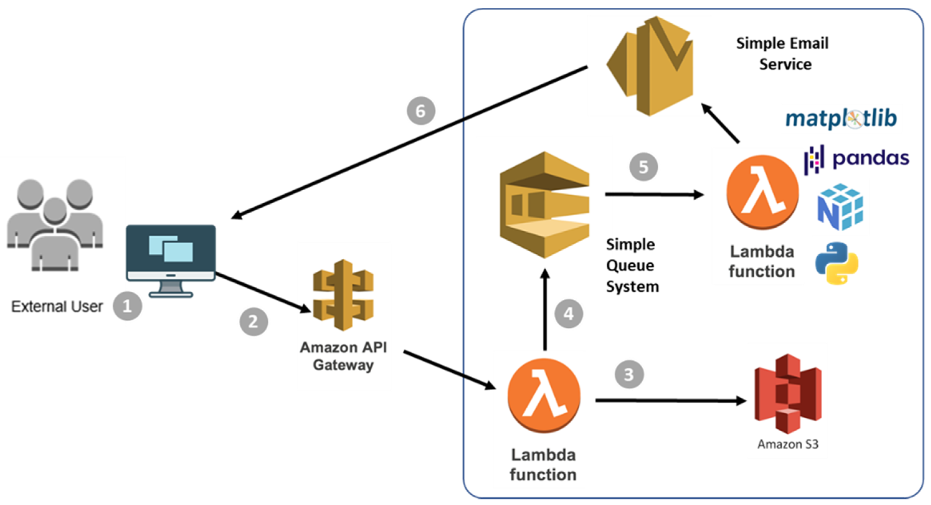
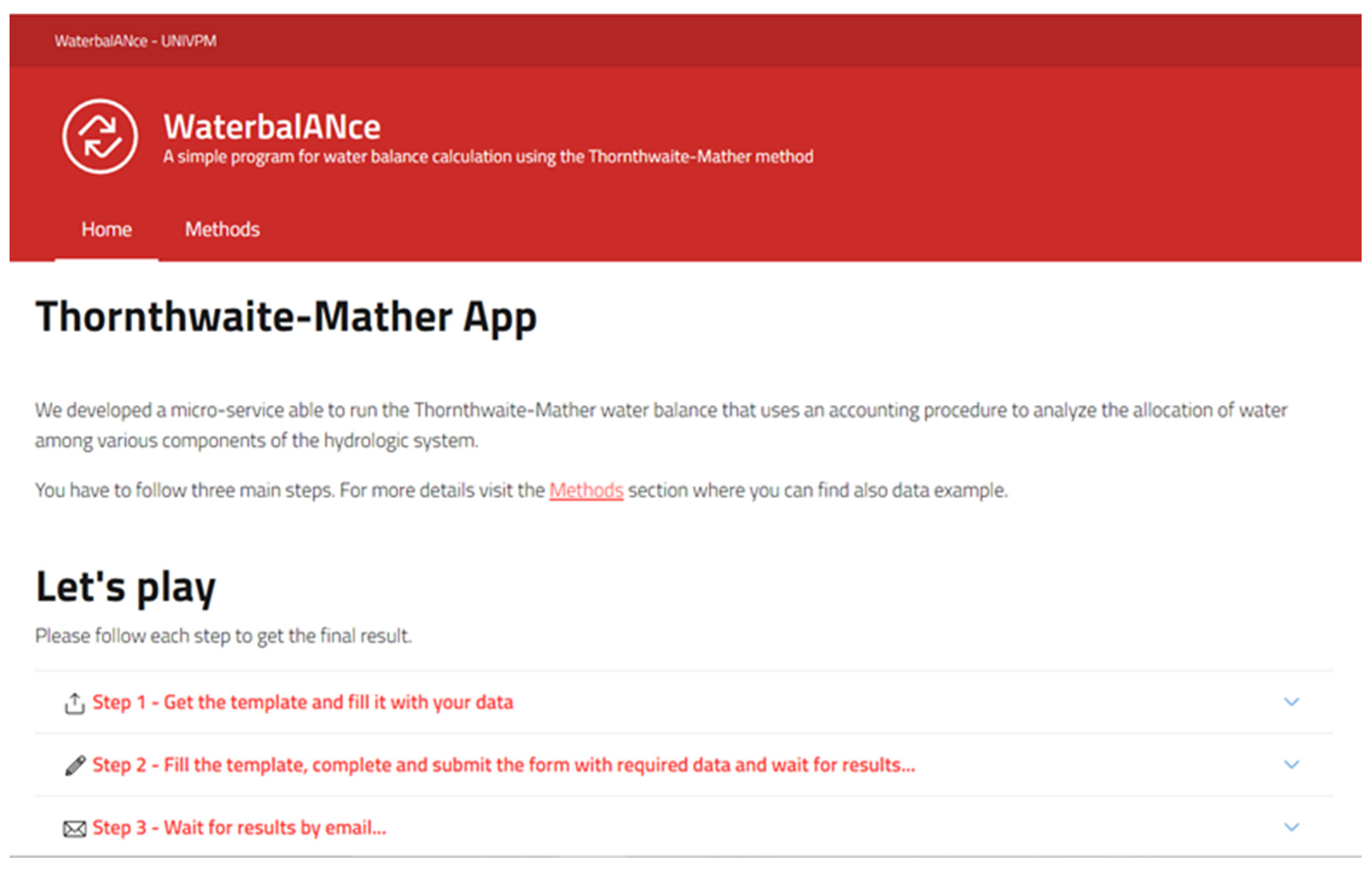
2.2. Exporting Algorithm to the Cloud

Today, the serverless computing approach is transforming attitudes towards computing. In particular, the serverless approach is widely used in common applications but is attracting the attention of scientists owing to its capability of allocating resources in real time according to the number of requests/users, as reported in [31,32]. Several service providers offer function-as-a-service (FaaS) solutions that could be used also for scientific computation. A set of functions could be easily exposed to the cloud owing to the availability of different runtime environments, such as Python, NodeJS, .NET core, and Java. In particular, the use of Python by scientists is increasing, and this is demonstrated by the wide availability of code and notebooks written in Python. The ability to convert programmed functions or methods into ready-to-use cloud services is leading to a seemingly serverless development and deployment experience for application software engineers. Without the necessity of allocating resources beforehand, the prototyping of new features and workflows is becoming faster and more convenient for application service providers. These advantages have served to boost the industry trend consequently called serverless computing. The more precise, almost overlapping term in accordance with everything-as a-service (XaaS) cloud computing taxonomies is function-as-a-service (FaaS).

The first implementation of the algorithm was performed in MATLAB. We decided to open up the application to external users, and the export of MATLAB code directly to the cloud is not straightforward. For this reason, we decided to port the code into the Python language using libraries such as numpy, matplotlib, and pandas. After the porting, we designed a cloud architecture based on the serverless approach to reduce the complexity as much as possible in order to maintain and scale the computing. The development of a WebApp simplifies the interaction with users, who are focused on the analysis of data without installing additional software modules. Figure 2 shows the adopted architecture that relies on cloud-based services. In particular, the user provides the required information through the front-end (see Figure 3): (a) LAT; (b) SM; (c) beta; (d) P; (e) Tm.

Data are uploaded according to a template that we provide to the end-user. In this phase, the application interacts with API gateway that triggers the lambda function. The lambda function stores the file in a storage service (S3). After the file is stored, the algorithm is executed using a custom layer on the lambda function to include the required dependencies mentioned above. At the end of execution, the final report is stored in the cloud storage, and using a simple notification system service, a message is sent to the end-user, allowing them to retrieve the results in a format such as an Excel spreadsheet file and a graphical plot (Figure 4). In this way, it is possible to scale the processing of multiple requests. We decided to send the results by using an e-mail considering that the user wishes to start the processing in an asynchronous way, without actively waiting. We decided to use the lambda function as limits in terms of resources (e.g., memory) for our application were expected. An alternative approach in the case of large datasets could rely on an on-demand node that could be activated and managed by Kubernetes as a task, but for our scenario, this configuration was not applicable. We also released the source code under the GNU GPLv3 license as a public git-hub repository (public repository used to share the code developed in the context of this work can be accessed via the following URL: https://github.com/vrai-group/thornwaterbalance accessed on 12 January 2021) for users who wish to integrate the developed algorithm into their pipeline.

2.3. The Practical Case of the Reno at Pracchia Watershed (Northern Apennines, Central Italy)

The first application of the model was performed on a watershed with a drainage are of roughly 39.8 km², located in the highest region of the Reno river (Northern Apennines, Italy), upstream of Pracchia village (610 m a.s.l.). Its maximum elevation is approximately 1640 m a.s.l., while the basin’s mean elevation is around 890 m a.s.l. From a geological point of view, the catchment is characterized by the lithologies of the Tuscan Nappe and Cervarola Unit (Figure 5). The Tuscan Nappe Unit crops out extensively in the Northern Apennines and comprises a calcareous to shaly succession (Triassic–Oligocene) and, at the top the Macigno Fm. (Upper Oligocene–Lower Miocene), a thick arenaceous turbidite succession that is late Oligocene–Early Miocene in age. The Cervarola Unit (Lower–Middle Miocene) covers broad areas of the Northern Apennines and is mainly formed by a thick arenaceous turbidite succession. The permeability of these lithologies is mainly driven by widespread tectonic deformation, demonstrated by extensive fracturing [33]. Consequently, the hydrogeological framework consists of small springs, with a local groundwater recharge system emerging from the passage between the sandstone and marly and clay lithologies [34]. The area is characterized by uniform morphometric setting, and due to its small size and the scarce anthropization around the riverbed, it is well suited to this type of analysis. The watershed is equipped for total rainfall and temperature and river discharge measurements, and the devices are owned by Servizio Idrometeorologico—ARPA Emilia Romagna Region; the daily and the mean monthly temperature, precipitation, and river discharge have been monitored and published in the Annali Idrologici reports (Part I, Part II) since 1968. Two different, continuous discharge datasets for the Apennines watershed were selected: the first covered January 1971 to December 1976 (Series I) and the second covered January 2008 to December 2018 (Series II). A descriptive statistical analysis was conducted (

Table 1. Descriptive statistics and comparison of modelled vs. measured discharge basic statistical parameters (Series I and Series II). Values refer to mean monthly calculation.

	Series I (January 1971–December 1976 Period)					Series II (January 2008–December 2018 Period)
	Mean	Min	Max	Std	Median	Mean	Min	Max	Std	Median
Modelled discharge (m3/s)	1.572	0.004	5.945	1.285	1.621	1.389	0.000	6.550	1.633	0.827
Measured discharge (m3/s)	1.591	0.108	7.145	1.362	1.345	1.599	0.050	8.610	1.771	0.845
Tm (°C)	9.9	0.9	22.0	6.0	8.85	10.9	−0.5	22.3	6.2	10.7
P (mm)	155.4	27.9	496.4	94.5	133.7	136.4	4.6	576.8	127.8	96.85

).

To run the model and to provide an example to the WebApp stakeholders (presented in the “Methods” section of the WebApp), the LAT, SM, SRT, and beta parameters were set based on expert knowledge of the geographical, geological, and climatic features of the area [35]. Respectively, LAT = 43 degrees, the SM = 200 mm, SRT = −1 °C and beta = 70%. Starting with TOT RO (mm) obtained as output, the modelled discharge (m³/s) was calculated by multiplying the latter with the drainage area (39.8 km²).

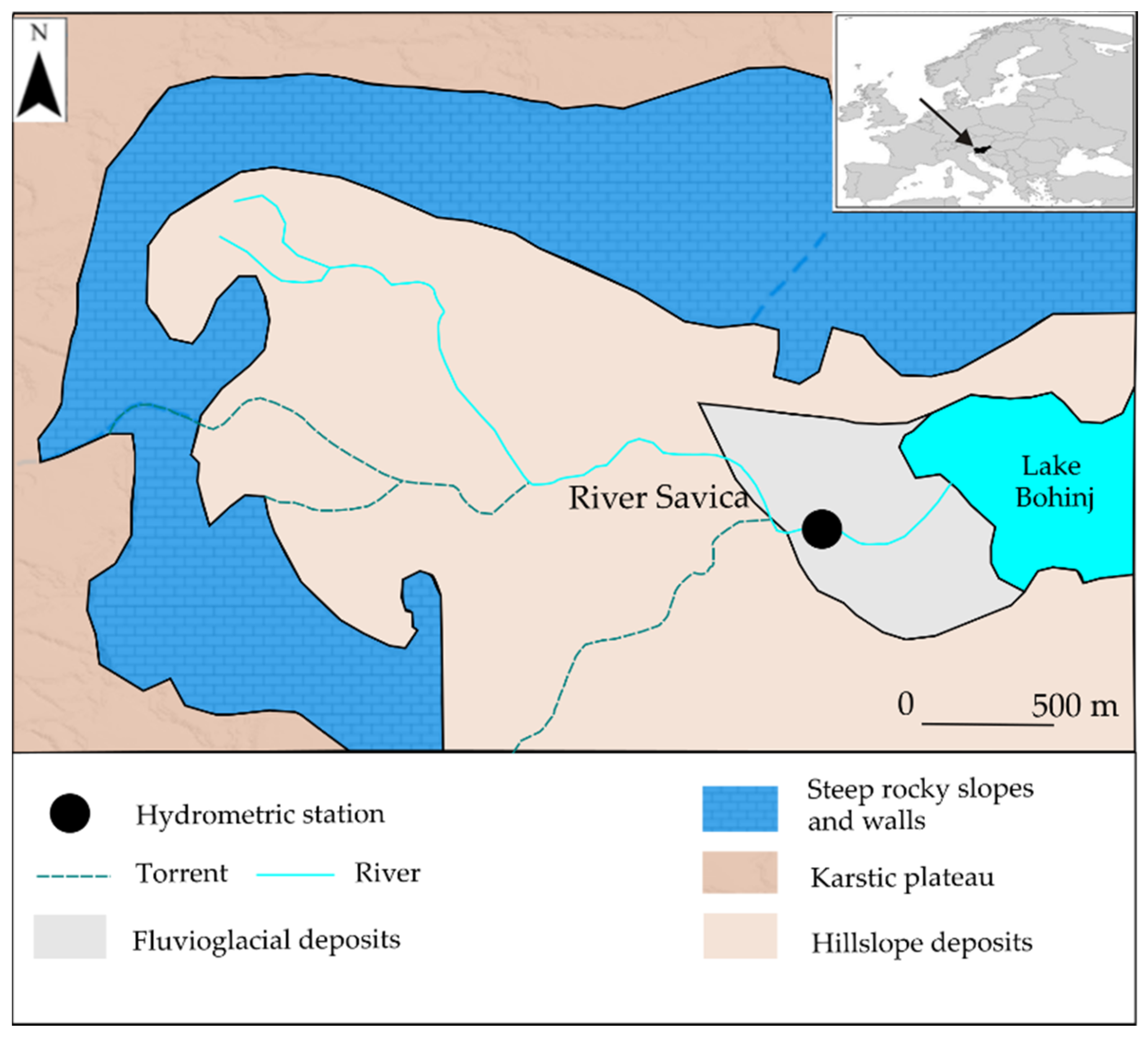
2.4. The Practical Case of the Savica at Ukanc Watershed (Northwestern Slovenia)

The second application of the WebApp was performed on the highest region of the Savica river (Northwestern Slovenia, Figure 6).

The drainage area is roughly 67 km², and it extends from 520 to 2800 m a.s.l. [37]. The river provides the main recharge of Bohinj Lake, the largest natural lake in Slovenia, and it is one of the two main sources of the River Sava, which constitutes the main trans-boundary river basin in the West Balkans and is part of the Danube basin [36]. From a geological point of view, the catchment is predominantly Dachstein limestone of Upper Triassic age, subordinated by a small number of dolomite beds [38]. In accordance with many other authors [39,40,41], the main river recharge area is positioned on the high karstified mountainous plateau that extends into the rugged high mountain chain. Data on river discharge are available only at the gauging station, Savica Ukanc (Elev: 528.83 m a.s.l), which is positioned 720 m before the confluence of the river with Bohinj Lake. Rainfall measurements are provided by the Slovenian Environmental Agency, and the rainfall station gauge available in the watershed is Bohinjska Cesnjica. LAT, SM, SRT, and beta parameters were set, respectively, to: LAT = 46 degrees, the SM = 100 mm, SRT = −1 °C, and beta = 50%. Starting with TOT RO (mm) obtained as output, the modelled discharge (m³/s) was calculated by multiplying the latter with the drainage area.

We emphasize that in both applications, SM and beta are not calibrated. Modelled discharge values were compared to the measured values by using Pearson’s coefficient of determination (R²), a standard means of measuring the error of a model in predicting quantitative data. The application of the model to the Reno at Pracchia watershed was also validated in a mean annual hydrologic year. This option can be set directly through the graphical user interface (Figure 3). Moreover, to identify if the discrepancy between measured and modelled discharge is linked to the peculiar meteoclimatic conditions, the difference between measured and modelled discharge data was plotted against the mean monthly precipitation (Figure 9).

3. Results and Discussion

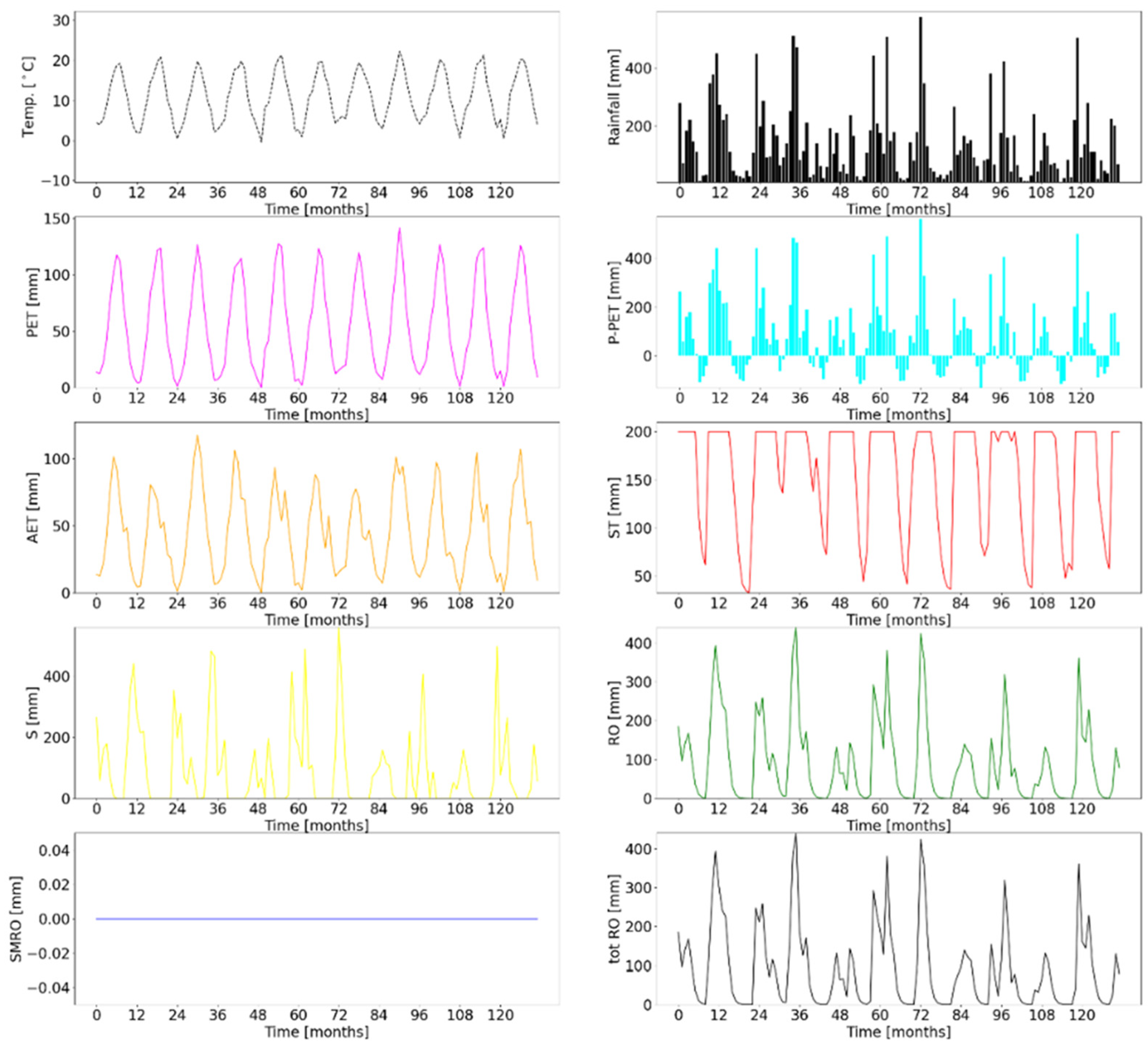
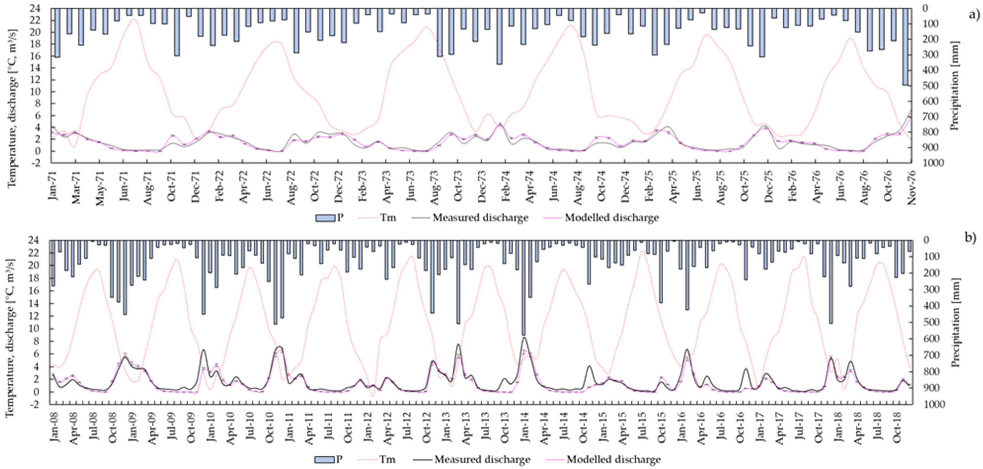
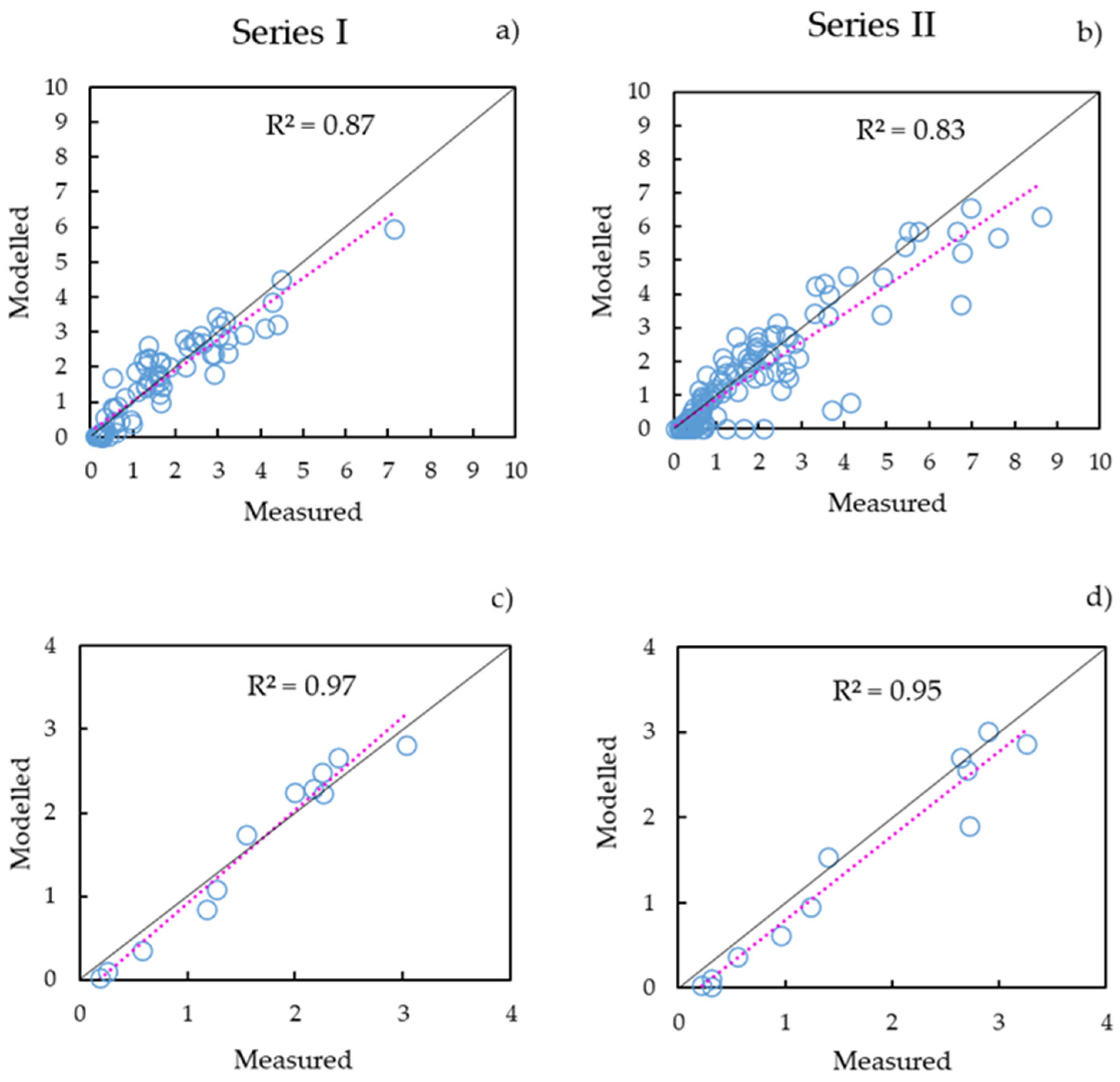
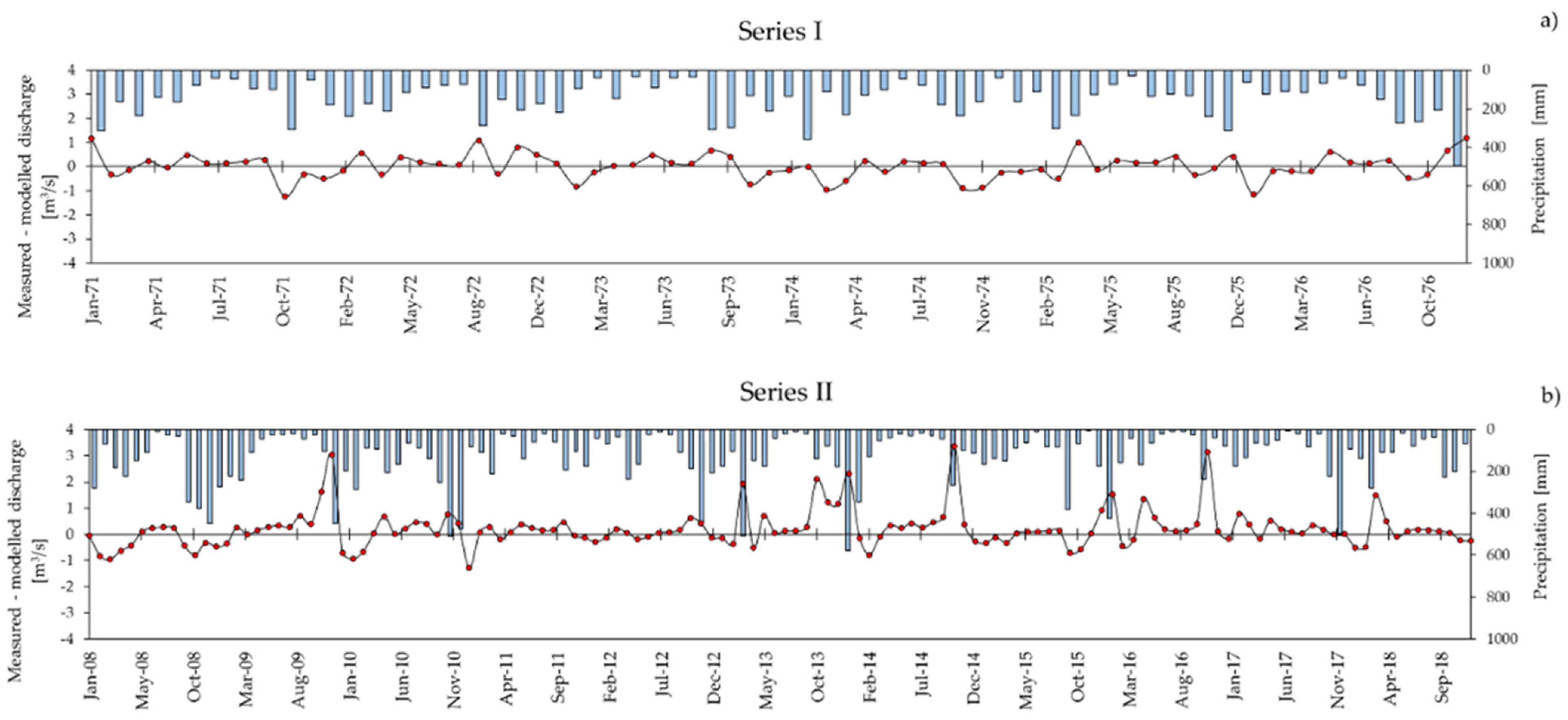
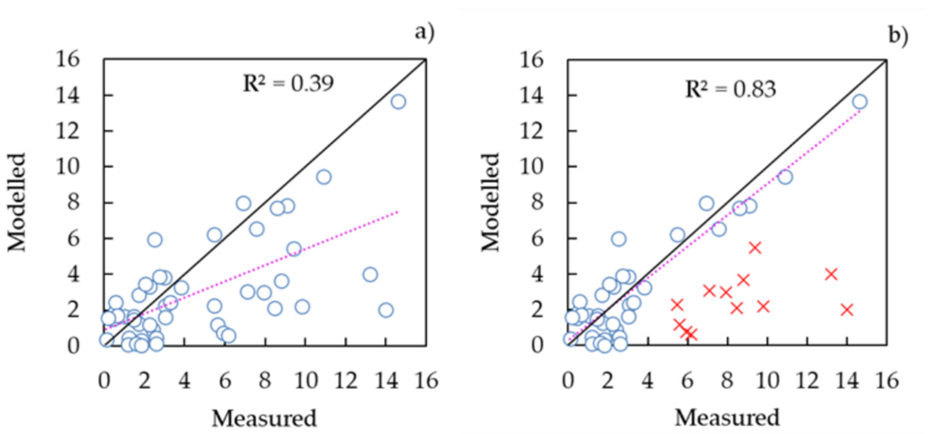
3.1. Reno at Pracchia Watershed

For each time series, mean monthly modelled discharge values with an associated error of 5% were compared to the observed values (Figure 7).

In Figure 8a,b, mean monthly measured discharge data are plotted against the modelled data. The correlation is slightly stronger for Series I (R² = 0.87) with respect to Series II (R² = 0.83). This result is also evidenced by Figure 9a, for which the difference between measured and modelled discharge is close to zero for all the observed periods. Regarding Series II, the larger differences between measured and modelled data were collected during the rainiest months (e.g., November 2009, 2014, 2016, and December 2013). In all these periods, we observe a positive difference of around 2 cubic meters, always suggesting a higher measured discharge with respect to the modelled value (Figure 9b). This finding could be connected to extreme rainfall events that occurred after prolonged dry periods.

Regarding the correlation of discharge data calculated in a mean hydrological year (Figure 8c,d), the Series I again demonstrates a slightly stronger correlation (R² = 0.97) with respect to Series II (R² = 0.95), both stronger than the monthly results.

The choice of SM and beta parameters, although not calibrated, have led to good simulation of the flow rates of the Reno at Pracchia watershed.

Table 1 shows the basic statistical results for the analyzed time series, with particular attention given to the model’s results and the hydrological conditions during the monitoring period. As supported by the Pearson’s coefficient of determination (Figure 7), the measured and modelled statistical parameters are extremely similar to one another. For instance, the mean discharge values for both the time series are quite similar (1.572 m³/s vs. 1.591 m³/s in Series I and 1.389 m³/s vs. 1.599 m³/s in Series II), also confirmed by the median values.

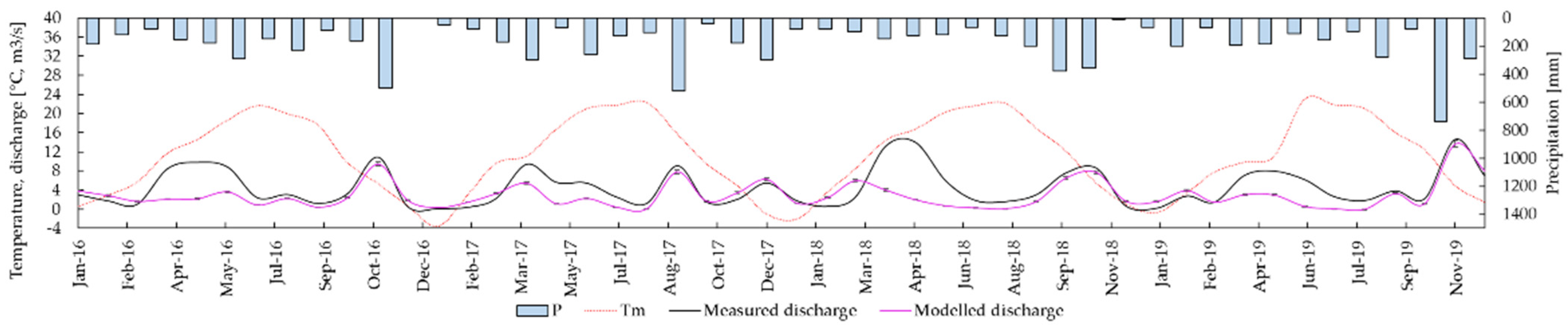
3.2. Savica at Ukanc Watershed

The results for the Savica at Ukanc watershed, presented in Figure 10, highlight the good performance of the Thornthwaite–Mather method during the winter and autumn seasons, while a discrepancy between modelled and measured discharge was observed between April and June.

Descriptive statistics of the temperature and precipitation data used as input in the model, coupled with basic statistics of mean monthly modelled discharge vs. measured discharge, are shown in

Table 2. Descriptive statistics of meteorological data and comparison of modelled vs. measured discharge basic statistical parameters. Values refer to mean monthly calculation.

	Mean	Min	Max	Std	Median
Modelled discharge (m3/s)	2.957	0.023	13.683	2.814	2.155
Measured discharge (m3/s)	4.544	0.098	14.610	3.886	2.876
Tm (°C)	11.2	−3.5	23.1	7.8	11.2
P (mm)	179.4	0.0	739.0	140.4	150

.

Considering the correlation between the mean monthly measured and modelled discharge data of the whole dataset from January 2016 to December 2019 (Figure 11a), Pearson’s correlation coefficient is equal to 0.39. If the period between April and June for each year (red crosses in Figure 11b) is not considered, R² is equal to 0.83. This behavior can be explained by the underestimation of the precipitation that falls in solid form using the rain gauge available in the watershed. This discharge regime is classified in accordance with [42], as predominately dominated by snow melting; then, the rainfall’s contribution to the water balance is subordinated.

Regarding the applicability of the Thornthwaite–Mather method, although some limitations to its use are reported in the literature. For instance, the method is usually applied where the geological site is characterized by the presence of soil cover [43], but in a few cases, it has been used in soil-less environments such as karst limestone aquifers [44,45].

In our study, the discharge data for the Reno at Pracchia watershed are quite well simulated (particularly in Series I) using the Thornthwaite–Mather method. In contrast, the Savica at Ukanc watershed, which is affected by the underestimation of snowfall and snow melting, is not a suitable area for which to simulate river discharge in the period between April and June.

4. Conclusions

The implementation of a WebApp for automatic water balance calculation allows the users to more efficiently carry out computation for large datasets. End-users will be provided with a template where data can be easily uploaded. The use of a serverless approach also represents a new means of processing data in case of scientific use. Data (input and output) are managed through several cloud services decoupling each component, also enabling automatic scalability. An Excel spreadsheet file and a graphical plot are sent to the users by e-mail, allowing the process to be run several times using different input parameters. Thanks to this automatic procedure for water balance calculation, it is possible to more quickly test the applicability of the Thornthwaite–Mather method in different geological and hydrogeological contexts and to discuss the important issue, which deserves to be studied in greater depth. In fact, in contrast to the classic MS Excel spreadsheet file, where time is proportional to the amount of data, the use of a WebApp permits the execution of the Thornthwaite–Mather method in a few minutes, regardless of the amount of input data. Moreover, no additional software modules need to be installed, and this simplifies the interaction with the final user, who can focus on the analysis of data. The availability of the source code as a public git-hub repository is useful for users who wish to integrate the developed algorithm into their pipeline. Future improvements of the WebApp may involve consideration of fraction of monthly precipitation that becomes snow, the function of the temperature, geographic location, elevation, and the aspect, as suggested by [46], in addition to testing the method in different contexts. For example, particular attention should be paid to the infiltration process in the soil or even in soil-less situations to improve the calibration of input parameters. The soil moisture storage capacity (SM) and the beta parameters, which influence the model discharge performance, should be improved by an automatic calibration procedure in order to minimize the associated mean absolute error between modelled and measured discharge. Once the calibration is performed on a basin with certain physical characteristics (e.g., soil and crop type, land use, morphometric characteristics, and lithology), the parameters obtained can aid in the simulation of the discharges of ungauged watersheds for water management.

References

1. Donker, N.H.W. WTRBLN: A computer program to calculate water balance. Comput. Geosci. 1987, 13, 95–122. [Google Scholar] [CrossRef]
2. Thornthwaite, C.W.; Mather, J.R. The Water Balance; Laboratory in Climatology, Johns Hopkins University: Baltimore, MD, USA, 1955; Volume 8, pp. 1–104. [Google Scholar]
3. Thornthwaite, C.W.; Mather, J.R. Instructions and Tables for Computing Potential Evapotranspiration and the Water Balance; Laboratory in Climatology, Johns Hopkins University: Baltimore, MD, USA, 1957; Volume 10, pp. 181–311. [Google Scholar]
4. Sepaskhah, A.R.; Razzaghi, F. Evaluation of the adjusted Thornthwaite and Hargreaves-Samani methods for estimation of daily evapotranspiration in a semi-arid region of Iran. Arch. Agron. Soil Sci. 2009, 55, 51–66. [Google Scholar] [CrossRef]
5. Bonacci, O.; Andrić, I. Karst spring catchment: An example from Dinaric karst. Environ. Earth Sci. 2015, 74, 6211–6223. [Google Scholar] [CrossRef]
6. Pelton, W.L.; King, K.M.; Tanner, C.B. An Evaluation of the Thornthwaite and Mean Temperature Methods for Determining Potential Evapotranspiration 1. Agron. J. 1960, 52, 387–395. [Google Scholar] [CrossRef]
7. Pruitt, W.O. Evapotranspiration: A guide to irrigation. Calif. Turfgrass Cult. 1964, 14, 27–32. [Google Scholar]
8. Doorenbos, J.; Pruitt, W.O. Crop Water Requirements; FAO Irrigation and Drainage Paper No. 24; FAO: Rome, Italy, 1977; pp. 34–37. [Google Scholar]
9. Hashemi, F.; Habibian, M.T. Limitations of temperature-based methods in estimating crop evapotranspiration in arid-zone agricultural development projects. Agric. Meteorol. 1979, 20, 237–247. [Google Scholar] [CrossRef]
10. Malek, E. Comparison of alternative methods for estimating ETp and evaluation of advection in the Bajgah area, Iran. Agric. For. Meteorol. 1987, 39, 185–192. [Google Scholar] [CrossRef]
11. Camargo, A.P.; Marin, F.R.; Sentelhas, P.C.; Picini, A.G. Adjust of the Thornthwaite’s method to estimate the potential evapotranspiration for arid and superhumid climates, based on daily temperature amplitude. Rev. Bras. Agrometeorol. 1999, 7, 251–257. [Google Scholar]
12. Scozzafava, M.; Tallini, M. Net infiltration in the Gran Sasso Massif of central Italy using the Thornthwaite water budget and curve-number method. Hydrogeol. J. 2001, 9, 461–475. [Google Scholar] [CrossRef]
13. Nanni, T.; Rusi, S. Idrogeologia del massiccio carbonatico della montagna della Majella (Appennino centrale). Bollettino-Società Geologica Italiana 2003, 122, 173–202. [Google Scholar]
14. Sellinger, C.E. Computer Program for Estimating Evapotranspiration Using the Thornthwaite Method; NOAA Technical Memorandum ERL GLERL-101; United States Department of Commerce: Washington, DC, USA, 1996.
15. Armiraglio, S.; Cerabolini, B.; Gandellini, F.; Gandini, P.; Andreis, C. Calcolo informatizzato del bilancio idrico del suolo. Nat. Brescia. Ann. Mus. Civ. Sci. Nat. Brescia 2003, 33, 209–216. [Google Scholar]
16. McCabe, G.J.; Markstrom, S.L. A Monthly Water-Balance Model Driven by a Graphical User Interface (Vol. 1088); US Geological Survey: Reston, VA, USA, 2007.
17. Hamon, W. Estimating potential evapotranspiration. Trans. Am. Soc. Civ. Eng. 1963, 128, 324–338. [Google Scholar] [CrossRef]
18. Di Matteo, L.; Dragoni, W. Climate change and water resources in limestone and mountain areas: The case of Firenzuola Lake (Umbria, Italy). In Proceedings of the 8th Conference on Limestone Hydrogeology, Neuchatel, Switzerland, 21–23 September 2006. [Google Scholar]
19. Di Matteo, L.; Dragoni, W.; Maccari, D.; Piacentini, S.M. Climate change, water supply and environmental problems of headwaters: The paradigmatic case of the Tiber, Savio and Marecchia rivers (Central Italy). Sci. Total Environ. 2017, 598, 733–748. [Google Scholar] [CrossRef] [PubMed]
20. Portela, M.M.; Santos, J.; de Carvalho Studart, T.M. Effect of the Evapotranspiration of Thornthwaite and of Penman-Monteith in the Estimation of Monthly Streamflows Based on a Monthly Water Balance Model. In Current Practice in Fluvial Geomorphology-Dynamics and Diversity; IntechOpen: Rijeka, Croatia, 2019. [Google Scholar]
21. Vandewiele, G.L.; Win, N.L. Monthly water balance models for 55 basins in 10 countries. Hydrol. Sci. J. 1998, 43, 687–699. [Google Scholar] [CrossRef]
22. Mather, J.R. The Climatic Water Budget in Environmental Analysis; Free Press: Wong Chuk Hang, Hong Kong, 1978. [Google Scholar]
23. Mather, J.R. Use of the climatic water budget to estimate streamflow. In Use of the Climatic Water Budget in Selected Environmental Water Problems; Elmer, N.J., Ed.; C.W. Thornthwaite Associates, Laboratory of Climatology: Centerton, NJ, USA, 1979; Volume 32, pp. 1–52. [Google Scholar]
24. McCabe, G.J.; Wolock, D.M. Independent effects of temperature and precipitation on modeled runoff in the conterminous United States. Water Resour. Res. 2011, 47. [Google Scholar] [CrossRef]
25. Pinna, M. Climatologia, XV ed.; UTET: Torino, Italy, 1977; p. 442. [Google Scholar]
26. Dooge, J.C.I. The rational method for estimating flood peaks. Engineering 1957, 184, 311–313, 374–377. [Google Scholar]
27. Schaake, J.C.; Geyer, J.C.; Knapp, J.W. Experimental examination of the rational method. J. Hydraul. Div. 1967, 93, 353–370. [Google Scholar] [CrossRef]
28. Boughton, W.C. Evaluating Partial Areas of Watershed runoff. J. Irrig. Drain. Eng. 1987, 113, 356–366. [Google Scholar] [CrossRef]
29. Longobardi, A.; Villani, P.; Grayson, R.B.; Western, A.W. On the relationship between runoff coefficient and catchment initial conditions. In Proceedings of the MODSIM, Townsville, Australia, 14–17 July 2003; pp. 867–872. [Google Scholar]
30. Ferguson, R.I. Snowmelt runoff models. Prog. Phys. Geogr. 1999, 23, 205–227. [Google Scholar] [CrossRef]
31. Spillner, J.; Mateos, C.; Monge, D.A. Faaster, better, cheaper: The prospect of serverless scientific computing and hpc. In Proceedings of the Latin American High-Performance Computing Conference, Buenos Aires, Argentina, 20–22 September 2017; Springer: Cham, Switzerland, 2017; pp. 154–168. [Google Scholar]
32. Pawlik, M.; Figiela, K.; Malawski, M. Performance considerations on execution of large-scale workflow applications on cloud functions. arXiv 2019, arXiv:1909.03555. [Google Scholar]
33. Cervi, F.; Corsini, A.; Doveri, M.; Mussi, M.; Ronchetti, F.; Tazioli, A. Characterizing the recharge of fractured aquifers: A case study in a flysch rock mass of the northern Apennines (Italy). In Engineering Geology for Society and Territory-Volume 3; Springer: Cham, Switzerland, 2015; pp. 563–567. [Google Scholar]
34. Tazioli, A.; Cervi, F.; Doveri, M.; Mussi, M.; Deiana, M.; Ronchetti, F. Estimating the isotopic altitude gradient for hydrogeological studies in mountainous areas: Are the low-yield springs suitable? Insights from the northern Apennines of Italy. Water 2019, 11, 1764. [Google Scholar] [CrossRef] [Green Version]
35. Valigi, D. La Simulazione Delle Portate Mensili nei Bacini in Facies di Flysch dell’Appennino Centro-Settentrionale con Particolare Riguardo al F. Nestore. Ph.D. Thesis, Università degli Studi di Perugia, Perugia, Italy, 1995. [Google Scholar]
36. Brenčič, M.; Vreča, P. Hydrogeological and isotope mapping of the karstic River Savica in NW Slovenia. Environ. Earth Sci. 2016, 75, 651. [Google Scholar] [CrossRef]
37. Ogrinc, N.; Kanduč, T.; Stichler, W.; Vreča, P. Spatial and seasonal variations in δ18O and δD values in the River Sava in Slovenia. J. Hydrol. 2008, 359, 303–312. [Google Scholar] [CrossRef]
38. Buser, S. Basic geological map of SFRJ 1:100,000. In Guidebook of Sheets Tolmin and Videm (Udine): L 33–63, 33–64; Zvezni Geološki Zavod, Beograd: Ljubljana, Slovenian, 1986. [Google Scholar]
39. Trišič, N.; Bat, M.; Polajnar, J.; Pristov, J. Water balance investigations in the Bohinj region. In Tracer Hydrology 97, Proceedings of the 7th International Symposium on Water Tracing, Portorož, Slovenia, 26–31 May 1997; CRC Press: Boca Raton, FL, USA, 1997; pp. 26–31. [Google Scholar]
40. Urbanc, J.; Brancelj, A. Tracing experiment in lake Jezero v Ledvici, valley Triglavska jezera. Geologija 1999, 42, 207–214. [Google Scholar] [CrossRef]
41. Bat, M. Hidrološke raziskave ARSO na območju Bohinja. Dela 2007, 165–181. [Google Scholar] [CrossRef]
42. Brenčič, M.; Vreča, P. Influence of snow thawing regime changes on the outflow from karstic aquifer. In Proceedings of the EGU General Assembly Conference Abstracts, Vienna, Austria, 7–12 April 2013. [Google Scholar]
43. Dourado-Neto, D.; Jong van Lier, Q.D.; Metselaar, K.; Reichardt, K.; Nielsen, D.R. General procedure to initialize the cyclic soil water balance by the Thornthwaite and Mather method. Sci. Agric. 2010, 67, 87–95. [Google Scholar] [CrossRef] [Green Version]
44. Dragoni, W.; Giontella, C.; Melillo, M.; Cambi, C.; Di Matteo, L.; Valigi, D. Possible response of two water systems in Central Italy to climatic changes. Adv. Watershed Hydrol. 2015, 397–424. [Google Scholar]
45. Guardiola-Albert, C.; Martos-Rosillo, S.; Pardo-Igúzquiza, E.; Duran Valsero, J.J.; Pedrera, A.; Jiménez-Gavilán, P.; Linan Baena, C. Comparison of recharge estimation methods during a wet period in a karst aquifer. Groundwater 2015, 53, 885–895. [Google Scholar] [CrossRef]
46. Legates, D.R.; Bogart, T.A. Estimating the proportion of monthly precipitation that falls in solid form. J. Hydrometeorol. 2009, 10, 1299–1306. [Google Scholar] [CrossRef]
Figure 1. Workflow of the WaterbalANce code. P = monthly precipitation (mm); Tm = mean monthly temperature (°C); LAT = latitude (°); SM = soil moisture storage capacity value (mm); beta = dimensionless runoff coefficient (%); SRT = snowfall rainfall threshold (°C); PET = monthly potential evapotranspiration (mm); delta = P-PET (mm); AET = monthly actual evapotranspiration (mm); ST = monthly soil moisture (mm); S = monthly water surplus (mm); RO = monthly runoff (mm); RES(i − 1) = dynamic water stored in the basin in the previous month (mm); RES = dynamic water storage available for the next month (mm); SMRO = monthly snow melt runoff (mm); TOT RO = monthly total runoff (mm).
Hydrology 08 00034 g001
Figure 2. Graphical representation of the adopted architecture to manage the WaterbalANce application. The architecture is based on the interconnection of lambda functions and cloud services to perform the computation.
Hydrology 08 00034 g002
Figure 3. Developed front-end using a standard (adopted for Italian application) to interact with the end-user to specify the parameters and upload the data [https://italia.github.io/bootstrap-italia/ accessed on 12 January 2021].
Hydrology 08 00034 g003
Figure 4. Example of the output plots. Months are plotted against the inputs (P, Tm) and output variables of the program.
Hydrology 08 00034 g004
Figure 5. Geological sketch map of the Reno at Pracchia watershed.
Hydrology 08 00034 g005
Figure 6. Geological sketch map of Savica at Ukanc watershed (modified from [36]).
Hydrology 08 00034 g006
Figure 7. Comparison of mean monthly measured and modelled discharge, monthly precipitation, and mean monthly temperature data for time series I (a) and II (b).
Hydrology 08 00034 g007
Figure 8. Measured vs. modelled discharge data (m³/s) for each time series, Reno at Pracchia watershed. (a,b) all datasets for Series I and Series II, respectively; (c,d) mean annual hydrologic year for Series I and II. The dashed line represents the linear data interpolation, while the black solid line is the reference line (1:1).
Hydrology 08 00034 g008
Figure 9. Measured minus modelled discharge and precipitation for time series I (a) and II (b).
Hydrology 08 00034 g009
Figure 10. Comparison of mean monthly measured and modelled discharge, monthly precipitation, and mean monthly temperature data for Savica at Ukanc.
Hydrology 08 00034 g010
Figure 11. Mean monthly measured vs. modelled discharge data (m3/s) for Savica at Ukanc watershed. (a) All datasets; (b) discarding the months between April and June for each year (red crosses). The dashed line represents the linear data interpolation, while the black solid line is the reference line (1:1).
Hydrology 08 00034 g011