Surface and Groundwater Interactions: A Review of Coupling Strategies in Detailed Domain Models


1
Environmental Systems Engineering, Faculty of Engineering and Applied Science, University of Regina, Regina, SK S4S 0A2, Canada
2
Hydrology and Groundwater Services, Saskatchewan Water Security Agency, Moose Jaw, SK S6H 7X9, Canada
*
Author to whom correspondence should be addressed.
Hydrology 2021, 8(1), 35; https://0-doi-org.brum.beds.ac.uk/10.3390/hydrology8010035
Submission received: 30 December 2020
/
Revised: 13 February 2021
/
Accepted: 14 February 2021
/
Published: 23 February 2021
Abstract
:In groundwater numerical simulations, the interactions between surface and groundwater have received great attention due to difficulties related to their validation and calibration due to the dynamic exchange occurring at the soil–water interface. The interaction is complex at small scales. However, at larger scales, the interaction is even more complicated, and has never been fully addressed. A clear understanding of the coupling strategies between the surface and groundwater is essential in order to develop numerical models for successful simulations. In the present review, two of the most commonly used coupling strategies in detailed domain models—namely, fully-coupled and loosely-coupled techniques—are reviewed and compared. The advantages and limitations of each modelling scheme are discussed. This review highlights the strategies to be considered in the development of groundwater flow models that are representative of real-world conditions between surface and groundwater interactions at regional scales.
1. Introduction
Water security is an emergent issue in the world due to climate change and variability, and increasing water demands due to population growth and economic development [1]. Both surface water and groundwater are, inevitably, resources that are needed in order to meet future water demands. Groundwater is widely used in the national economies of many countries for different purposes, such as potable and industrial water supply, irrigation, and mineral water. Fresh groundwater is of particular importance as the main source of public water in the domestic and drinking water balance. To date, groundwater is the main source of potable water in most European countries and in the United States, which accounts for 75% of municipal water supply system [2]. Irrigation has grown rapidly over the past 50 years, and approximately 40% of the irrigated regions of the world are predominantly governed by groundwater resource [3]. However, in recent years, the depletion of groundwater has become a concern due to overexploitation. A greater understanding is needed to better manage the limited water resources, especially in drought-prone areas. There is a need to better understand the interactions between groundwater and surface water, which is fundamentally an integrated feature in the hydrologic cycle. These interactions could be influenced by both natural and anthropogenic processes [4]. Recently, research has focused on the proper selection of models that accounts for surface and groundwater interactions coupled into a single framework. However, there are many restrictions associated with this approach. There are considerable fluctuations of surface and groundwater interactions at the soil–water interface due to the heterogeneous nature of the porous medium with time, along with the variabilities due to climate change. The diversity of aquifer types, along with recharge and groundwater flow conditions, and the extensive range of river flow circumstances provide the ingredients for a complex system of interactions, which heightens the need for robust modelling and solution methodologies [5].
Surface water models are being used to understand surface water systems by including possible deviations due to both natural and human influences. The interrelation and coupling among various subsystems of the hydrological cycle has been noted by many pioneer researchers in the process of the physical and mathematical description of the flow processes [6]. The first physically-based and coupled model, Système Hydrologique Européen (SHE), was developed primarily based on fundamentals of surface water flow. The United States Geological Survey (USGS) PRMS (Precipitation-Runoff Modelling System) and National Oceanic and Atmospheric Administration (NOAA)’s National Weather Service models [7] are the recent developments of surface water models. The groundwater flow models have the ability to simulate predicted impacts from over-exploitation, to simulate the fate and transport of a contaminate plume, and to forecast the variation of the groundwater levels with time due to climatic variability. However, the traditional groundwater flow models neglect the incorporation of surface water flux into the subsurface environment. MikeSHE and SHETRAN were further developed and applied with both surface and groundwater flow [8,9,10].
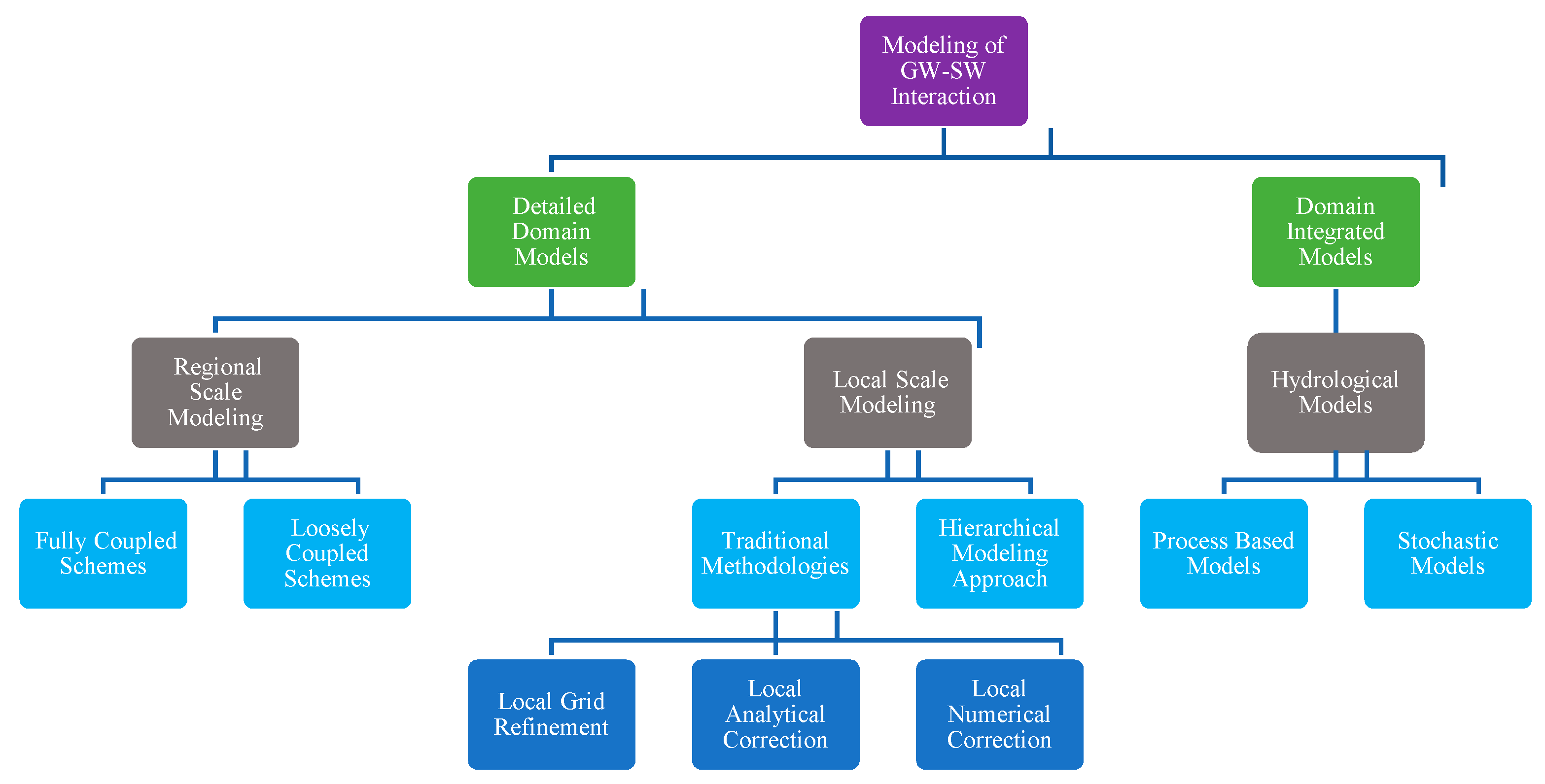
From the literature, it has been noticed that the modelling and simulation of groundwater and surface water interaction have been conducted by many researchers [11,12,13,14]. Multiple factors have been reported that could influence the interaction between ground and surface water, such as hydro-climatic variables; physiographic structure; differences in the head between the catchment surface water and groundwater; and the surface and groundwater flow geometry [15,16]. The modeling of flows and transport phenomena as discrete groundwater systems has been achieved well by relatively simpler approaches [15,17]. However, the modelling process is complicated by the inclusion of surface water and groundwater interaction. Ever-present interactions between groundwater and surface water are a concern due to the continuous flow of groundwater into rivers [5]. The integration of groundwater and surface water interaction could be classified in many different ways. Figure 1 illustrates a schematic of the different available modelling approaches. It serves as the foundation and framework for the present review. The objectives of the present review are to compare the coupling strategies in detailed domain models, which are the fully-coupled and loosely-coupled schemes. The domain integrated modelling will be briefly reviewed and compared to detailed domain models.
2. Detailed Domain Models
Detailed domain models have been developed on surface and groundwater simulation. For the regional scale modelling, the fully-coupled and loosely-coupled schemes are the two widely used techniques. The traditional methodologies and the hierarchical modelling approach will be addressed within the local scale modelling discussion.
2.1. Regional Scale Modelling
A regional scale is defined as a catchment with an area between 1000 and 10,000 km2. It can include variables such as climate, geology, geomorphology, landscape categories, and biological and human factors in the same region [18,19,20]. The surface and groundwater interaction on the regional scale incorporates the entire terrestrial hydrological cycle using observations at larger distances and simplified interaction processes. Fully- and loosely-coupled schemes are the two widely used techniques in regional scale modelling.
2.1.1. Fully-Coupled Scheme
Fully-coupled schemes are physically-based models that integrate the surface and groundwater components of the hydrologic cycle into a single software package. A fully-coupled scheme software package has the ability to solve governing equations for both surface and groundwater flow simultaneously. Fully-coupled models can investigate the interaction over a range of spatial and temporal scales. Stable results can be acquired by these models [7], resulting in a reduction in the number of ancillary software packages needed to address the various subsystems [21,22]. In fully-coupled systems, the governing equations for groundwater flow are based on the modified Richards’ equation for both saturated and unsaturated zones. The governing equation for surface water is based on the depth-averaged Saint-Venant equation given below.
Governing Equations
Richards’ equation describes the conservation of the mass of the water phase in the void space in the porous medium, along with Darcy’s equation for the volumetric flux given below.
- Porous Medium (3D) Richards’ Equation:
- Darcy–Buckingham Equation:
where, (dimensionless) is the volumetric division of the total porosity of the porous medium (or the primary continuum); = source/sink rate, which defines the volumetric fluid flux per unit volume demonstrating a source (positive) or a sink (negative) to the porous medium system = exchange fluxes term= degree of water saturation; = porosity; = pressure head; z = elevation head; is the permeability tensor; and (dimensionless) is the relative permeability (function of saturation). The hydraulic conductivity tensor, [] = where is the water viscosity [], g is the acceleration due to gravity [], is the permeability tensor of the porous medium [L2], and is the water density [], which is a function of the concentration C [] of any particular solute, such that . The water saturation is interconnected to the moisture content (dimensionless) according to . In Equation (2), ex represents the exchange rate of the volumetric fluid between the subsurface domain and all of the other categories of domains supported by the model, and it is expressed per unit volume of the other domain types. Generally, these additional domains are surface, tile drains, wells, discrete fractures, and dual continuum. The definition of ex (positive for the flow into the porous medium) relies on the conceptualization of fluid exchange between the domains [23].
The depth-averaged Saint-Venant equation for surface water can be written as:
where = source/sink rate, = water depth; = exchange fluxes; h0 = surface hydrostatic pressure. Incorporating the Manning equation relating the flux with the gradient of the surface water system, it can be written as:
where is roughness, is the surface water gradient, and = relative permeability. The surface and subsurface flows are coupled through interaction terms that represent the flux interchange between the two surface–subsurface compartments [23,24].
It has been hypothesized that the first-order exchange term can be calculated using
where h is the subsurface pressure head, is the conductance at the surface/subsurface interface, and is the coupling-relative permeability/rill storage.
Fully-coupled software packages are based on three separate coupling strategies for the integration of hydrostatic surface water (i.e., Saint-Venant) and subsurface flow: first-order exchange, continuity of pressure and boundary condition switching [25]. A first-order exchange formulation or conductance has been applied for the coupling of surface and groundwater flow equations in HydroGeoSphere (HGS) and InHM software packages. The flux continuity can be maintained, and the continuity of pressure can then be imposed across the surface and subsurface domains [26,27]. The first-order exchange approach is based on Darcy’s Law for flow through an exchange interface. The surface and groundwater exchange flux (positive/negative as exfiltration/infiltration) is linearly dependent on the difference between the subsurface head at the uppermost node, and the surface head, as well as the value of the first-order exchange or conductance coefficient [27]. This mechanism has been used in investigations pertaining to flow simulation between different continua, such as fractures and macropores, rock and soil, and river–aquifer interactions through streambeds.
In another coupling strategy, the continuity of pressure coupling formulation is introduced and incorporated into the ATS (Advanced Terrestrial Simulator), Cast3M, and ParFlow software packages. These packages are fully-coupled models with a free-surface overland boundary condition on the top, based on pressure and flux continuity at the surface [28,29,30]. The surface water equations were used for the interface conductance [31].
The boundary condition switching coupling strategy has been used in CATHY software to enforce flux and pressure continuity at the surface/subsurface interface. This approach acts as a special treatment in variably-saturated subsurface flow models to detect atmosphere-controlled and soil-limited infiltration and evaporation dynamics [28]. It translates potential atmospheric fluxes into actual fluxes across the land surface, and the resulting surface storage [32,33]. A common hypothesis in these approaches is to maintain pressure and flux continuity at the surface/subsurface interface while ignoring the continuity of momentum and forces.
A limited number of regional applications using fully-coupled models can be found in the literature, including its applications on small scales [34]. As one of the fully-coupled models, the Penn State Integrated Hydrologic Model (PIHM) was developed with a reservoir simulation module. PIHM can be converted into an optimization model under the Simulation-Optimization (S-O) modelling structure [35]. The Simulation-Optimization (S-O) modelling approach has been extensively recognized to resolve complications in water resources management [36,37,38,39,40,41,42,43,44]. The main idea of S-O modelling is to build interconnectivity between a simulation model and optimization scheme so that a trade-off between groundwater extraction rates and surface water reduction can be established. A fully-coupled model was also tested for lake-dominated hydrologic regimes with natural fluctuations, such as landscape disturbance. This integrated approach has been applied in spatially-distributed atmospheric flux information, including evapotranspiration, throughfall, and landscape diversity, in order to imitate field observations. However, it is recommended that the groundwater recharge rate and timing should be pre-defined between evapotranspiration and temporal throughfall fluid. Hence, groundwater recharge is being considered as a governing factor for the maintenance of lakes and wetlands by the use of the fully-coupled method [45].
The advantages of the fully-coupled scheme are also very clear. It has been found that the simulation results have a good agreement with the experimental/observed field data. The fully-coupled models can also be used for coastal and lake simulations. Additionally, this technique has been validated based on the large number of available software packages from previous studies. However, as noted, the fully-coupled approach should not be used in unsaturated zones with overbearing lateral flow [46]. In order to improve the accuracy of fully-coupled models, it is suggested that the quasi-adaptive meshing configuration should be adopted without considering the total number of grids. The quasi-adaptive meshing offers flexibilities to correct local discretization inaccuracies due to the topographic elevation grade [47]. In short, the fully-coupled models can serve as a strong watershed simulator for the examination of watershed hydrological characteristics with the desired accuracy.
Many pieces of software can be found using fully-coupled schemes. The dynamic interactions between the surface and subsurface are captured in a seamless way. However, the new parameters that appear in the flow equation with the coupling term should be determined experimentally or by fitting exercises. Table 1 lists examples of software packages that are fully-coupled models.
With the application of the fully-coupled schemes, there are some disadvantages to the approach. There has been a lack of studies in the application of the fully-coupled approach at a regional scale. This limitation is likely due to the robustness of the software packages addressing the surface–groundwater interactions at the catchment scale. A direct comparison of the simulation results using different software is not practical. Most of the evaluations have been completed on local scales with limited testing and applicability to the real-world environment. The application of fully-coupled approaches on larger scales has not been extensively tested due to the complexity of the interactions between surface water and groundwater [34]. Another disadvantage of the fully-coupled models is the lengthy computational time. The calibration of the model is another challenge due to the large number of estimated parameters. The boundary and the initial conditions could also introduce larger uncertainties, resulting in high computational effort and cost. It is critical to scale up and down for simulations using the fully-coupled models [57].
2.1.2. Loosely-Coupled Scheme
The surface and groundwater can be solved individually by using a loosely-coupled scheme, either in succession without iteration, or iteratively within each time step. Two or more separate models could be used in this approach. There are many loosely-coupled models that were developed in the past that depended on these techniques [25].
Governing Equations
In the subsurface, the governing equations are derived from Darcy’s law, with the continuity equation [58]. The mass conservation equation for a confined aquifer can be written as (Mehdinejadiani et al., 2013):
where is piezometric head; is time, , and are the principal components of the hydraulic conductivity tensor; and is specific storage.
For an unconfined aquifer [58]:
Solving the equations for unconfined groundwater flow is complicated due to the fluctuations of the aquifers’ thickness and variations, which could occur due to the withdrawal of groundwater [33,59]. The Dupuit principle and Boussinesq equation can be used to address this issue [60,61]. For loosely-coupled models, the coupling technique should be strong enough to transfer the data spatially and temporally [61]. Many of the loosely-coupled models have been established for specific catchments. It should be noted that some extra terms can be added to the governing equations, which should be solved by infiltration models. Infiltration models offer a systematic framework to understand the unsaturated zone and the groundwater flow. Many infiltration models had been established in the past. Green–Ampt, Horton’s, Philip’s, and Holtan’s are some of the well-known infiltration models.
A loosely-coupled scheme has been implemented with a direct linkage from hydrogeological data to hydrogeological numerical models in GIS, such as ArcArAz [55]. Unstructured meshes have been shown to be a unique characteristic in loosely-coupled models to simplify the boundary conditions. The efficiency of the loosely-coupled approach has been tested well in complex hydrological processes. The output of the surface water model has been applied as an imposed flux for groundwater recharge rates in MODFLOW [62]. It is also noted that some parameters, such as groundwater recharge rates, have the capacity to connect groundwater and surface water models. The importance of the transition zone between surface and groundwater flow has been noted from previous simulation results [62].
The loosely-coupled scheme has some advantages, such as the flexibility to apply individual tools to each environmental process, rather than one tool for all of the processes. This approach offers alternative software to reuse the hydrogeological conceptual model in GIS [55]. Similarly, the loosely-coupled scheme provides preference options in determining the platform to be used for any definite stage [63].
Several loosely-coupled frameworks have been developed for regional scales. However, there are some disadvantages, such as the difficulty in obtaining concrete decisions from the evaluation based on previous studies, because each structure was implemented for a particular catchment. The other disadvantages of the loosely-coupled scheme include the lack of a proper methodology to evaluate groundwater models. The groundwater model calibration is not sufficient for transient models with different recharge rates. The consideration of the transition zone is only possible by the construction of a fully-integrated dynamic model, which has two directional linkages between the surface and groundwater [62,64]. The geological properties of regional aquifers are normally simplified as heterogeneous in the estimation of spatial distribution of groundwater recharge. For this reason, the application of loosely-coupled models is extremely problematic, especially in the context of regional-scale modelling [65,66,67,68]. Convergence could be a challenging concern in the case of nonlinear models, including iteratively coupled models [7]. Inadequate statistics and information with respect to the interpolation of river water levels between gauges always creates difficulties when dealing with the measurement of the exchange term based on pressure differences [34]. For the estimation of exchange fluxes relying on pressure variances, the determination of river stages through the interpolation between the gauges is required, but loosely-coupled models are incapable of calculating river water levels at any point along the reach of a river. Apart from these above-mentioned complications, complexities in loosely-coupled models might also arise due to insufficient data of riverbed elevations with respect to a common datum (sea level) in potentially relevant stretches where the channel bottom would have to be derived using proxy data.
To date, MIKE SHE and FEFLOW, coupled with MIKE11 are the most commonly used loosely-coupled models for regional studies. Some loosely-coupled models are listed in Table 2.
2.2. Local Scale Modelling
Local scale modelling is applied for smaller spatial areas for surface and groundwater interaction. The cross section of the river can be incorporated in a particular small region with simplifications of other processes outside the research area. However, the influence of these outside processes could vary, and may play a significant role in determining the interaction. Thus, boundary conditions should be carefully defined, such as the groundwater recharge, runoff formation, and regional groundwater flow [34].
2.2.1. Traditional Methodologies
Several traditional techniques have been used in local scale modelling, including local grid refinement, local analytical correction, and local numerical correction [88]. In the following, these three techniques will be briefly reviewed.
Local grid refinement is one of the most common methods for well dynamics prediction. The resolution of the grid is dependent on the domain and knowledge of the local geology/hydrogeology [89,90,91]. Two or more distinctly sized grids have been associated with local grid refinement, in which a coarse grid occupying a huge area with the inclusion of regional boundary settings and one or more finer grids enclose the local areas. A one-way coupling methodology can be used to establish the link between the coarse and fine grids. In this approach, the conditions simulated by the coarse grid are applied into the fine boundaries, or through the process of two-way feedback between the two grids [92]. Table 3 highlights some of the advantages and disadvantages of this methodology.
The local analytical correction method was developed using a finite difference scheme. This technique is characterized by better enhancement for the forecasting of drawdown in the pumping well, which can be compared to the exact solution [94,95]. However, this corrected drawdown method would not be applicable in several realistic scenarios, such as for multiple sources and sinks within the well block with variable hydraulic conductivity, anisotropic media with detailed coordination, variable recharge, fractional well penetration, and transient flow or pumping circumstances [96,97,98,99,100].
The local numerical correction is based on the subdivisions of moderately large finite-difference grid cells from a regional model into multiple cells with gradually smaller spatial dimensions. This technique can be applied continuously until the preferred resolution of the well scale is achieved. It can be performed as an independent model after the creation of the local model. Restrictive assumptions of the local analytical correction and potential complications associated with local grid refinement can be avoided in this method. The conversion of facts and figures from a regional to a local model, and the choice of the initial and final boundary conditions for the generated local model have been identified as the most significant issues in this approach. As such, the use of multiple smaller-scale local models instead of resolving very large, complex matrices has been implemented under this process. This approach has the capability to minimize a huge and difficult matrix system into multiple smaller and improved conditioned matrices [88]. However, this approach could be very time consuming with the introduction of new boundary conditions or scales.
2.2.2. Hierarchical Modelling Approach
The hierarchical approach is an interactive and periodic technique, which is primarily based on the nested grid method [88]. It has the capability to address some of the disadvantages in the traditional methodologies by using dynamically coupled and fully integrated settings [94]. A dynamically integrated hierarchical patch dynamics paradigm (HPDP) has been established for groundwater modelling. This approach has some unique features, such as reduced assumptions, data input and post-processing, which significantly improve its calculating efficiency. The simulation results for regional model and groundwater systems are satisfactory without solving large matrix structures [67,90]. This approach also raises confidence in estimating exchange fluxes [100]. The dynamic fusion policy in the model has made real-time integration and subscale modelling possible. Computation steering application within the approach can be applied to manipulate the simulation process.
Furthermore, a computational steering application within this approach is able to provide the platform for human intelligence, allowing for human interruption during the time of execution, with modifications in the final output, such as the addition of patches in particular areas and layers of concern [66]. In short, the permission to focus indeterminately into a specific zone as long as the governing equations can maintain a certain scale is one of the vital advantages of this modelling strategy. The hierarchical approach is a realistic and time-efficient way to carry out complicated hydrological field settings. However, extensive data in a well-recognized structure is required for this process. The users may need a physical illustration of the database. Hierarchical structures have the tendency to adapt slowly to changing requirements. This system includes data to be frequently stored in many different entities. The limitations of this approach include deficiencies of structural independence, as well as a complex navigation scheme [101,102].
3. Domain Integrated Modelling
Domain integrated modelling is used for a simplification of the water cycle. Both the water quantity and water quality can be forecast. Two types of domain integrated models can be named: process-based models and stochastic models.
3.1. Process-Based Models
Process-based models can be referred to as deterministic hydrology models which incorporate all of the physical processes from the real world. This type of model uses streamflow, surface runoff, subsurface flow, etc. in individual-event models and continuous simulation models. Some of the highlights from previous studies using process-based models can be found in the following section.
Process-based models have been applied to represent the hydrological and ecological cycle in prairie wetlands [103]. The impacts of different water budget constituents were identified. Lateral contribution as runoff from the individual wetlands and their respective catchments were considered to be a fully integrated hydrological system. The prairie wetland region is hydraulically interconnected to the shallow aquifer systems, with continual flow exchange between precipitation, surface water and groundwater. The permanence of the wetland ponds has been proposed as another important criterion, which usually relies on factors such as runoff inputs and the hydrological position within a landscape, etc. The function of the artificial drainage of wetlands is critical to flooding, stream-water quality, and groundwater recharge.
A physically-based and distributed interaction model has been applied for greenhouse gas emission scenarios. The temporal dynamics of surface and groundwater interaction under climate change have been numerically investigated. From the simulation results, the impact of groundwater on stream flow is significant under climate change scenarios [104]. In order to improve the representation of surface and groundwater interaction, a groundwater model known as ‘CLASS’ has been developed. The interaction of surface and groundwater has been further established, including water table dynamics and land surface parameters. Other experimentally-based simulations, such as CK, CK-GW and CK-GWL have been included in the CLASS model in order to identify the impacts of regional hydrology variations. Among these, CK-GWL was significantly modified in the past few years in order to improve the accountability of subsurface lateral flow in addition to recharge and discharge processes. Many studies have used the CK-GWL model to simulate surface runoff, stream flows, wetter soil moistures, and a high water table [24]. However, the application and results obtained from statistical principles recommended further investigations using the regional climate model for better simulations of soil moisture and stream flows through the inclusion of the groundwater component in land surface modelling. Some other research has been conducted to identify the main reasons for groundwater fluctuations [105]. It was noted that groundwater level fluctuation is a combined consequence of many parameters, including direct and induced recharge, the extraction rate, and lateral groundwater flow, etc.
3.2. Stochastic Models
Stochastic models are developed like a black box by using mathematical and statistical theories to create a linkage between input data and the model’s output. Regression, neural networks, transfer functions, system identification are some of the methodologies that have been used in stochastic modelling. The application of these techniques is reviewed in the following.
Time series modelling is one of the most well-known strategies to estimate hydrogeological properties, e.g., flow and storage issues. This modelling approach has been applied due to its accuracy and cost-efficiency [106,107,108,109]. Multi-annual groundwater records can be used to describe aquifer properties. However, delayed gravity yield can generate erroneous groundwater hydrographs in time series modelling. The errors are evident in well pumping events at the initial time, which can be minimized by incorporating this effect into a transfer function model. Future research should be conducted to investigate the efficiency of this modelling approach [110]. The regression method is another technique that has been widely used in previous studies to investigate the groundwater table and groundwater management [111,112,113]. For instance, short-term groundwater table fluctuations have been generated using a triple linear regression method. The interrelationship among all of the key parameters in the determination of groundwater fluctuations can be established. It was found, from this regression and sensitivity analysis, that precipitation, evaporation, and river stages have the most significant role [114]. It is recommended that geographical locations and hydraulic conductivity should be considered in the determination of groundwater table variations using this method.
4. Discussion
The groundwater and surface water interaction is complex. A comprehensive framework is required in order to consider the climate, geological, and hydrological conditions. The interaction is critical for the successful simulation of groundwater research due to its direct influences on recharge–discharge approaches [63]. The interaction is desired to improve the modelling of groundwater and surface water. From the present review, it can be seen that the scale and uncertainty arise in the groundwater and surface water interactions. Temporal and spatial scales on both groundwater and surface water quantity and quality have not been addressed clearly [115]. Local and regional scale alterations and interchange have not been measured precisely. Therefore, the simulation results may vary significantly.
Various coupling techniques have been compared in the present review. Fully-coupled models can deliver an instantaneous clarification to groundwater and surface water interactions by combining process-based equations with 3D subsurface demonstrations. The fully-coupled model works best when the groundwater and surface water interactions are needed at a larger or regional scale, with the consideration of all of the hydrological processes. Fully-coupled models are most effective compared to other schemes in integrated systems. This approach also has the capacity to handle complex physics in regional scale modelling. However, the lack of field data in large-scale modelling has been a major hindrance for the successful application of fully-coupled models [116]. A large number of computational resources is needed for fully-coupled model simulation, due to the large number of estimated parameters. The calibration could be complicated, due to the high uncertainty in the boundary and initial conditions. Thus, a loosely-coupled approach has been used in the past with relatively simple coupling schemes.
Many loosely-coupled structures have been developed for local-scale modelling, especially for regional studies, such as MIKE SHE, FEFLOW coupled with MIKE 11. The loosely-coupled models can communicate one-way information to sub-models with mean coupled equations and feedbacks [117]. In this approach, the selection and integration of sub-models, such as groundwater, surface water and the unsaturated zone, results in the uncertainty of the modeled results due to variables in the input parameters within each of the sub-models. Some of the models are dependent on surface water models, while others are not. Additionally, the boundary placement between the coupling models is another challenge in loosely-coupled models.
5. Conclusions
Groundwater and surface water models can be integrated, but the terminology for the model coupling has yet to be defined well from the literature. Diverse coupling approaches need to be compared for future modelling applications. Fully-coupled models have the capabilities to resolve the Richards’ and shallow water equations simultaneously, and thereby can provide proper explanations of any complex physics scenario, as well as estimating the parameters for regional scale models. However, the large number of required parameters and a limited knowledge of the boundary conditions may increase the complexity. On the other hand, loosely-coupled methodologies based on empirical relationships can be used in a mixture of process-based models, or process-based models and other algorithms. The results from single models can be utilized as inputs for other models. Simplification in calibration and uncertainty evaluations are the main benefits of loosely-coupled models. Convergence difficulties for nonlinear models as well as disparities among the individual models during the time of their independent calibrations are some of the drawbacks of loosely-coupled models. Examples of software that were developed based on both fully-coupled and loosely-coupled models have been listed, which might help researchers choose the appropriate models when interaction flux needs to be considered. The models could be further classified by the boundaries at the interface between the groundwater, the vadose zone, and the surface water. The assumptions of all of the models could be simplified by reducing some of these uncertainties as well as the variable spatial and temporal features of the groundwater and surface water flows. A separate suitable framework is desired in order to address the uncertainties for future development.
Author Contributions
Conceptualization, A.H. and P.W.; Formal analysis, A.H., A.S., K.L.; Project administration, P.W.; Writing—original draft, A.H.; Writing—review and editing, A.S., K.L., P.W. All authors have read and agreed to the published version of the manuscript.
Funding
The research was funded by NSERC Discovery Grant.
Institutional Review Board Statement
Not Applicable.
Informed Consent Statement
Not applicable.
Data Availability Statement
Not applicable.
Acknowledgments
The authors are grateful for the comments from anonymous reviewers.
Conflicts of Interest
The authors declare no conflict of interest.
References
- Vaux, H. Groundwater under stress: The importance of management. Environ. Earth Sci. 2011, 62, 19–23. [Google Scholar] [CrossRef] [Green Version]
- Zektser, I.S.; Everett, L.G. Groundwater Resources of the World and Their Use; IHP-VI, Series on groundwater n°6; UNESDOC: Paris, France, 2004. [Google Scholar]
- Lejars, C.; Daoudi, A.; Amichi, H. The key role of supply chain actors in groundwater irrigation development in North Africa. Hydrogeol. J. 2017, 25, 1593–1606. [Google Scholar] [CrossRef]
- Toran, L. Groundwater–Surface Water Interaction. In Encyclopedia of Water: Science, Technology, and Society; Maurice, P.A., Ed.; John Wiley & Sons, Inc.: Hoboken, NJ, USA, 2019; pp. 1–12. [Google Scholar]
- Larocque, M.; Broda, S. Groundwater–surface water interactions in Canada. Can. Water Resour. J. Rev. Can. Ressour. Hydr. 2016, 41, 451–454. [Google Scholar] [CrossRef] [Green Version]
- Freeze, R.; Harlan, R. Blueprint for a physically-based, digitally-simulated hydrologic response model. J. Hydrol. 1969, 9, 237–258. [Google Scholar] [CrossRef]
- Great Lakes Science Advisory Board. Great Lakes Surface and Groundwater Model. Integration Review Literature Review, Options for Approaches and Preliminary Action Plan for the Great Lakes Basin Prepared by the Great Lakes Science Advisory Board Research Coordination Committee Submitted to rge Internation Join Commission. In Proceedings of the International Joint Commission Workshop Groundwater-Surface water modeling for the Great Lakes Basin, Ann Arbor, MI, USA, 4–5 April 2018. [Google Scholar]
- Abbott, M.B.; Bathurst, J.C.; Cunge, J.A.; O’Connell, P.E.; Rasmussen, J. An introduction to the European Hydrological System—Systeme Hydrologique Europeen, ‘SHE’, 1: History and philosophy of a physically-based, distributed modelling system. J. Hydrol. 1986, 87, 45–59. [Google Scholar] [CrossRef]
- Ewen, J.; Parkin, G.; O’Connell, P.E. SHETRAN: Distributed River Basin Flow and Transport Modeling System. J. Hydrol. Eng. 2000, 5, 250–258. [Google Scholar] [CrossRef] [Green Version]
- Abbott, M.B.; Bathurst, J.C.; Cunge, J.A.; O’Connell, P.E.; Rasmussen, J. An introduction to the European Hydrological System—Systeme Hydrologique Europeen, ‘SHE’, 2: Structure of a physically-based, distributed modelling system. J. Hydrol. 1986, 87, 61–77. [Google Scholar] [CrossRef]
- Mare, H.G.; Rademeyer, J.L.; Sami, K. Application on Groundwater/Surface water Interaction Modeling in the Schoonspruit Catchment. Available online: https://www.miya-water.com/fotos/artigos/02_application_on_groundwater_surface_water_interaction_modeling_in_the_schoonspruit_catchment_19810471915a326afa23030.pdf (accessed on 29 December 2020).
- Scibek, J.; Allen, D.M.; Cannon, A.J.; Whitfield, P.H. Groundwater-surface water interaction under scenarios of climate change using a high-resolution transient groundwater model. J. Hydrol. 2007, 333, 165–181. [Google Scholar] [CrossRef]
- Stefania, G.A.; Rotiroti, M.; Fumagalli, L.; Simonetto, F.; Capodaglio, P.; Zanotti, C.; Bonomi, T. Modeling groundwater/surface-water interactions in an Alpine valley (the Aosta Plain, NW Italy): The effect of groundwater abstraction on surface-water resources. Hydrogeol. J. 2017, 26, 147–162. [Google Scholar] [CrossRef]
- Pitz, C.F. Predicted Impacts of Climate Change on Groundwater Resources of Washington State; Ecology Publications & Forms: Washington, DC, USA, 2016. [Google Scholar]
- Rassam, D.W.; Jolly, I.; Pickett, T. Guidelines for Modelling Groundwater-Surface Water Interactions in EWater Source Towards Best Practice Model Application; eWater CRC: Bruce, Australia, 2012. [Google Scholar]
- Kumar, C.P. Modelling of Groundwater Flow and Data Requirements. Int. J. Mod. Sci. Eng. Technol. 2015, 2, 18–27. [Google Scholar]
- Kumar, C.P. Groundwater Modelling Software—Capabilities and Limitations. IOSR J. Environ. Sci. Toxicol. Food Technol. 2012, 1, 46–57. [Google Scholar] [CrossRef]
- Dahl, M.; Nilsson, B.; Langhoff, J.H.; Refsgaard, J.C. Review of classification systems and new multi-scale typology of groundwater-surface water interaction. J. Hydrol. 2007, 344, 1–16. [Google Scholar] [CrossRef]
- Winter, T.C.; Harvey, J.W.; Franke, O.L.; Alley, W.M. Ground Water and Surface Water: A Single Resource; US Geological Survey: Reston, VA, USA, 1998; Volume 10. [Google Scholar]
- Sophocleous, M. Interactions between groundwater and surface water: The state of the science. Hydrogeol. J. 2002, 10, 52–67. [Google Scholar] [CrossRef]
- Brunner, P.A.; Simmons, C.T. HydroGeoSphere: A Fully Integrated, Physically Based Hydrological Model. Ground Water 2011, 50, 170–176. [Google Scholar] [CrossRef] [Green Version]
- Loague, K.; Heppner, C.S.; Mirus, B.B.; Ebel, B.A.; Ran, Q.; Carr, A.E.; Beville, S.H.; VanderKwaak, J.E. Physics-based hydrologic-response simulation: Foundation for hydroecology and hydrogeomorphology. Hydrol. Process. 2006, 20, 1231–1237. [Google Scholar] [CrossRef]
- Therrien, R.; McLaren, R.G.; Sudicky, E.A.; Panday, S.M. HydroGeoSphere. A Three-Dimensional Numerical Model Describing Fully-Integrated Subsurface and Surface Flow and Solute Transport; Groundwater Simulations Group, University of Waterloo: Waterloo, ON, Canada, 2010; p. 457. [Google Scholar]
- Ganji, A.; Sushama, L. Improved representation of surface-groundwater interaction in the Canadian land surface scheme. Int. J. Clim. 2018, 38, 5077–5094. [Google Scholar] [CrossRef]
- Maxwell, R.M.; Putti, M.; Meyerhoff, S.B.; Delfs, J.-O.; Ferguson, I.M.; Ivanov, V.Y.; Kim, J.; Kolditz, O.G.; Kollet, S.J.; Kumar, M.; et al. Surface-subsurface model intercomparison: A first set of benchmark results to diagnose integrated hydrology and feedbacks. Water Resour. Res. 2014, 50, 1531–1549. [Google Scholar] [CrossRef] [Green Version]
- Maxwell, R.M.; Condon, L.E.; Kollet, S.J. A high-resolution simulation of groundwater and surface water over most of the continental US with the integrated hydrologic model ParFlow v3. Geosci. Model. Dev. 2015, 8, 923–937. [Google Scholar] [CrossRef] [Green Version]
- Liggett, J.E.; Werner, A.D.; Simmons, C.T. Influence of the first-order exchange coefficient on simulation of coupled surface-subsurface flow. J. Hydrol. 2012, 414–415, 503–515. [Google Scholar] [CrossRef]
- Kollet, S.J. The integrated hydrologic model intercomparison project, IH-MIP2: A second set of benchmark results to diagnose integrated hydrology and feedbacks Stefan. Water Resour. Res. 2017, 53, 867–890. [Google Scholar] [CrossRef] [Green Version]
- Kollet, S.J.; Maxwell, R.M.; Woodward, C.S.; Smith, S.; VanderBorght, J.; Vereecken, H.; Simmer, C. Proof of concept of regional scale hydrologic simulations at hydrologic resolution utilizing massively parallel computer resources. Water Resour. Res. 2010, 46, 1–7. [Google Scholar] [CrossRef]
- Maxwell, R.M. ParFlow User’s Manual. Ground Water 2010, 1, 129. [Google Scholar]
- Kollet, S.J.; Maxwell, R.M. Integrated surface–groundwater flow modeling: A free-surface overland flow boundary condition in a parallel groundwater flow model. Adv. Water Resour. 2006, 29, 945–958. [Google Scholar] [CrossRef] [Green Version]
- Camporese, M.; Paniconi, C.; Putti, M.; Orlandini, S. Surface-subsurface flow modeling with path-based runoff routing, boundary condition-based coupling, and assimilation of multisource observation data. Water Resour. Res. 2010, 46. [Google Scholar] [CrossRef] [Green Version]
- Furman, A. Modeling Coupled Surface-Subsurface Flow Processes: A Review. Vadose Zone J. 2008, 7, 741–756. [Google Scholar] [CrossRef] [Green Version]
- Barthel, R.; Banzhaf, S. Groundwater and Surface Water Interaction at the Regional-scale – A Review with Focus on Regional Integrated Models. Water Resour. Manag. 2016, 30, 1–32. [Google Scholar] [CrossRef] [Green Version]
- Seo, S.B.; Mahinthakumar, G.; Sankarasubramanian, A.; Kumar, M. Conjunctive management of surface water and groundwater resources under drought conditions using a fully coupled hydrological model. J. Water Resour. Plan. Manag. 2018, 144, 1–11. [Google Scholar] [CrossRef] [Green Version]
- Arena, C.; Mazzola, M.R.; Scordo, G. A simulation/optimization model for selecting infrastructure alternatives in complex water resource systems. Water Sci. Technol. 2010, 61, 3050–3060. [Google Scholar] [CrossRef] [PubMed] [Green Version]
- Giacomoni, M.H.; Joseph, J. Multi-Objective Evolutionary Optimization and Monte Carlo Simulation for Placement of Low Impact Development in the Catchment Scale. J. Water Resour. Plan. Manag. 2017, 143, 04017053. [Google Scholar] [CrossRef]
- Katsifarakis, K.; Petala, Z. Combining genetic algorithms and boundary elements to optimize coastal aquifers’ management. J. Hydrol. 2006, 327, 200–207. [Google Scholar] [CrossRef]
- Lund, J.R. Optimization modeling in water resource systems and markets. Water Trading Glob. Water Scarcity 2012, 341–353. [Google Scholar] [CrossRef]
- Mantoglou, A.; Papantoniou, M.; Giannoulopoulos, P. Management of coastal aquifers based on nonlinear optimization and evolutionary algorithms. J. Hydrol. 2004, 297, 209–228. [Google Scholar] [CrossRef]
- Rao, S.V.N.; Bhallamudi, S.M.; Thandaveswara, B.S.; Mishra, G.C. Conjunctive use of surface and groundwater for coastal and deltaic systems. J. Water Resour. Plan. Manag. 2004, 130, 255–267. [Google Scholar] [CrossRef] [Green Version]
- Safavi, H.R.; Darzi, F.; Mariño, M.A. Simulation-optimization modeling of conjunctive use of surface water and groundwater. Water Resour. Manag. 2010, 24, 1965–1988. [Google Scholar] [CrossRef]
- Shourian, A.J.; Raoufi, M. Interbasin water transfer capacity design by two approaches of simulation-optimization and multicriteria decision making. J. Water Resour. Plan. Manag. 2017, 143, 04017054. [Google Scholar] [CrossRef]
- Zekri, S.; Triki, C.; Al-Maktoumi, A.; Bazargan-Lari, M.R. An optimization-simulation approach for groundwater abstraction under recharge uncertainty. Water Resour. Manag. 2015, 29, 3681–3695. [Google Scholar] [CrossRef]
- Smerdon, B.D.; Mendoza, C.A.; Devito, K.J. Simulations of fully coupled lake-groundwater exchange in a subhumid climate with an integrated hydrologic model. Water Resour. Res. 2007, 43, 1–13. [Google Scholar] [CrossRef]
- Zhu, Y.; Shi, L.; Lin, L.; Yang, J.; Ye, M. A fully coupled numerical modeling for regional unsaturated-saturated water flow. J. Hydrol. 2012, 475, 188–203. [Google Scholar] [CrossRef]
- Takeuchi, J.; Kawachi, T.; Imagawa, C.; Buma, N.; Unami, K.; Maeda, S. A physically based FVM watershed model fully coupling surface and subsurface water flows. Paddy Water Environ. 2010, 8, 145–156. [Google Scholar] [CrossRef]
- Harter, T.; Morel-Seytoux, H. Peer Review of the IWFM, MODFLOW and HGS Model Codes: Potential for Water Management Applications in California’s Central Valley and Other Irrigated. Excell. Consens. Water. 2013, 2013, 121. [Google Scholar]
- Ashby, S.F.; Falgout, R.D. A Parallel Multigrid Preconditioned Conjugate Gradient Algorithm for Groundwater Flow Simulations. Nucl. Sci. Eng. 1996, 124, 145–159. [Google Scholar] [CrossRef]
- Jones, J.E.; Woodward, C.S. Newton–Krylov-multigrid solvers for large-scale, highly heterogeneous, variably saturated flow problems. Adv. Water Resour. 2001, 24, 763–774. [Google Scholar] [CrossRef] [Green Version]
- Delfs, J.; Sudicky, E.A.; Park, Y.; Mclaren, R.G. An inter-comparison of two coupled hydrogeological models. In Proceedings of the XIX International Conference on Water Resources, CMWR, Urbana-Champaign, IL, USA, 17–22 June 2012; pp. 1–8. [Google Scholar]
- Kolditz, O.; Bauer, S.; Bilke, L.; Böttcher, N.; Delfs, J.O.; Fischer, T.; Görke, U.J.; Kalbacher, T.; Kosakowski, G.; McDermott, C.I.; et al. OpenGeoSys: An open-source initiative for numerical simulation of thermo-hydro-mechanical/chemical (THM/C) processes in porous media. Environ. Earth Sci. 2012, 67, 589–599. [Google Scholar] [CrossRef]
- Guay, C.; Nastev, M.; Paniconi, C.; Sulis, M. Comparison of two modeling approaches for groundwater-surface water interactions. Hydrol. Process. 2013, 27, 2258–2270. [Google Scholar] [CrossRef]
- Muma, M.; Rousseau, A.N.; Gumiere, S.J. Assessment of the impact of subsurface agricultural drainage on soilwater storage and flows of a small watershed. Water 2016, 8, 326. [Google Scholar] [CrossRef] [Green Version]
- Alcaraz, M.; Vázquez-Suñé, E.; Velasco, V.; Criollo, R. A loosely coupled GIS and hydrogeological modeling framework. Environ. Earth Sci. 2017, 76. [Google Scholar] [CrossRef]
- Bisht, G.; Huang, M.; Zhou, T.; Chen, X.; Dai, H.; Hammond, G.E.; Riley, W.J.; Downs, J.L.; Liu, Y.; Zachara, J.M. Coupling a three-dimensional subsurface flow and transport model with a land surface model to simulate stream–aquifer–land interactions (CP v1.0). Geosci. Model Dev. 2017, 10, 4539–4562. [Google Scholar] [CrossRef] [Green Version]
- Fatichi, S.; Vivoni, E.R.; Ogden, F.L.; Ivanov, V.Y.; Mirus, B.; Gochis, D.; Downer, C.W.; Camporese, M.; Davison, J.H.; Ebel, B.; et al. An overview of current applications, challenges, and future trends in distributed process-based models in hydrology. J. Hydrol. 2016, 537, 45–60. [Google Scholar] [CrossRef] [Green Version]
- Bear, V.A. Modeling Groundwater Flow and Pollution; Springer Science & Business Media: Berlin/Heidelberg, Germany, 1987. [Google Scholar]
- Mehdinejadiani, B.; Jafari, H.; Baleanu, D. Derivation of a fractional Boussinesq equation for modelling unconfined groundwater. Eur. Phys. J. Spéc. Top. 2013, 222, 1805–1812. [Google Scholar] [CrossRef]
- Nimmo, J.R. Unsaturated Zone Flow Processes. Encycl. Hydrol. Sci. 2005, 10. [Google Scholar] [CrossRef]
- Bronstert, A.; Carrera, J.; Kabat, P.; Lütkemeier, S. (Eds.) Coupled Models for the Hydrological Cycle; Springer: Berlin/Heidelberg, Germany, 2005. [Google Scholar]
- Barth, C.; Krause, P.; Boyle, D.P.; Markstrom, S.L. Hydrologic modeling of a groundwater dominated watershed using a loosely coupled modeling approach. Int. Congr. Model. Simul. Adv. Appl. Manag. Decis. Making Proc. 2005, 2015, 601–607. [Google Scholar]
- Huang, G.; Yeh, G.-T. Comparative Study of Coupling Approaches for Surface Water and Subsurface Interactions. J. Hydrol. Eng. 2009, 14, 453–462. [Google Scholar] [CrossRef]
- Barthel, R. Common problematic aspects of coupling hydrological models with groundwater flow models on the river catchment scale. Adv. Geosci. 2006, 9, 63–71. [Google Scholar] [CrossRef] [Green Version]
- Bhattarai, M.P. Impact of Climate Change on Surface and Subsurface Water Interaction and Riparian Vegetation: Linkage between Hydrology and Invasive Tamarisk in a Semi-Arid Basin; University of Nevada: Reno, NV, USA, 2013. [Google Scholar]
- Jie, Z.; van Heyden, J.; Bendel, D.; Barthel, R. Combination of soil-water balance models and water-table fluctuation methods for evaluation and improvement of groundwater recharge calculations. Hydrogeol. J. 2011, 19, 1487–1502. [Google Scholar] [CrossRef]
- Wolf, J.; Barthel, R.; Braun, J. Modeling Ground Water Flow in Alluvial Mountainous Catchments on a Watershed Scale. Ground Water 2008, 46, 695–705. [Google Scholar] [CrossRef]
- Rivard, C.; Lefebvre, R.; Paradis, D. Regional recharge estimation using multiple methods: An application in the Annapolis Valley, Nova Scotia (Canada). Environ. Earth Sci. 2013, 71, 1389–1408. [Google Scholar] [CrossRef]
- Hu, L.; Zhang, M.; Yang, Z.; Fan, Y.; Li, J.; Wang, H.; Lubale, C. Estimating dewatering in an underground mine by using a 3D finite element model. PLoS ONE 2020, 15, e0239682. [Google Scholar] [CrossRef]
- Said, A.; Stevens, D.K.; Sehlke, G. Estimating water budget in a regional aquifer using hspf-modflow integrated model. J. Am. Water Resour. Assoc. 2005, 41, 1–42. [Google Scholar] [CrossRef]
- Wilcox, L.J.; Bowman, R.S.; Shafike, N.G. Evaluation of Rio Grande management alternatives using a surface-water/ground-water model. J. Am. Water Resour. Assoc. 2007, 43, 1595–1603. [Google Scholar] [CrossRef]
- Ragab, R.; Bromley, J.; Dörflinger, G.; Katsikides, S. IHMS-Integrated hydrological modelling system. Part 2. application of linked unsaturated, DiCaSM and saturated zone, MODFLOW models on Kouris and Akrotiri catchments in Cyprus. Hydrol. Process. 2010, 24, 2681–2692. [Google Scholar] [CrossRef]
- Ragab, R.; Bromley, J. IHMS-Integrated Hydrological Modelling System. Part 1. Hydrological processes and general structure. Hydrol. Process. 2010, 24, 2663–2680. [Google Scholar] [CrossRef]
- Hassan, S.M.T.; Lubczynski, M.W.; Niswonger, R.G.; Su, Z. Surface-groundwater interactions in hard rocks in Sardon Catchment of western Spain: An integrated modeling approach. J. Hydrol. 2014, 517, 390–410. [Google Scholar] [CrossRef]
- Niswonger, R.G.; Allander, K.K.; Jeton, A.E. Collaborative modelling and integrated decision support system analysis of a developed terminal lake basin. J. Hydrol. 2014, 517, 521–537. [Google Scholar] [CrossRef]
- Tian, Y.; Zheng, Y.; Wu, B.; Wu, X.; Liu, J.; Zheng, C. Modeling surface water-groundwater interaction in arid and semi-arid regions with intensive agriculture. Environ. Model. Softw. 2015, 63, 170–184. [Google Scholar] [CrossRef]
- Surfleet, C.G.; Tullos, D. Uncertainty in hydrologic modelling for estimating hydrologic response due to climate change (Santiam River, Oregon). Hydrol. Process. 2013, 27, 3560–3576. [Google Scholar] [CrossRef] [Green Version]
- Surfleet, C.G.; Tullos, D.; Chang, H.; Jung, I.W. Selection of hydrologic modeling approaches for climate change assessment: A comparison of model scale and structures. J. Hydrol. 2012, 464–465, 233–248. [Google Scholar] [CrossRef] [Green Version]
- Højberg, A.L.; Troldborg, L.; Stisen, S.; Christensen, B.B.S.; Henriksen, H.J. Stakeholder driven update and improvement of a national water resources model. Environ. Model. Softw. 2013, 40, 202–213. [Google Scholar] [CrossRef]
- Qin, H.; Cao, G.; Kristensen, M.; Refsgaard, J.C.; Rasmussen, M.O.; He, X.; Liu, J.; Shu, Y.; Zheng, C. Integrated hydrological modeling of the North China Plain and implications for sustainable water management. Hydrol. Earth Syst. Sci. 2013, 17, 3759–3778. [Google Scholar] [CrossRef] [Green Version]
- Habets, F.; Gascoin, S.; Korkmaz, S.; Thiéry, D.; Zribi, M.; Amraoui, N.; Carli, M.; Ducharne, A.; Leblois, E.; LeDoux, E.; et al. Multi-model comparison of a major flood in the groundwater-fed basin of the Somme River (France). Hydrol. Earth Syst. Sci. 2010, 14, 99–117. [Google Scholar] [CrossRef] [Green Version]
- Miller, N.L.; Dale, L.L.; Brush, C.F.; Vicuna, S.D.; Kadir, T.N.; Dogrul, E.C.; Chung, F.I. Drought Resilience of the California Central Valley Surface-Ground-Water-Conveyance System. JAWRA J. Am. Water Resour. Assoc. 2009, 45, 857–866. [Google Scholar] [CrossRef]
- Korkmaz, S.; Ledoux, E.; Önder, H. Application of the coupled model to the Somme river basin. J. Hydrol. 2009, 366, 21–34. [Google Scholar] [CrossRef]
- LeDoux, E.; Gomez, E.; Monget, J.; Viavattene, C.; Viennot, P.; Ducharne, A.; Benoit, M.; Mignolet, C.; Schott, C.; Mary, B. Agriculture and groundwater nitrate contamination in the Seine basin. The STICS–MODCOU modelling chain. Sci. Total. Environ. 2007, 375, 33–47. [Google Scholar] [CrossRef]
- Werner, A.D.; Gallagher, M.R.; Weeks, S.W. Regional-scale, fully coupled modelling of stream-aquifer interaction in a tropical catchment. J. Hydrol. 2006, 328, 497–510. [Google Scholar] [CrossRef]
- Kim, N.W.; Chung, I.M.; Won, Y.S.; Arnold, J.G. Development and application of the integrated SWAT-MODFLOW model. J. Hydrol. 2008, 356, 1–16. [Google Scholar] [CrossRef]
- Fleckenstein, J.H.; Niswonger, R.G.; Fogg, G.E. River-aquifer interactions, geologic heterogeneity, and low-flow management. Ground Water 2006, 44, 837–852. [Google Scholar] [CrossRef] [PubMed]
- Emara, N.A.; Hussein, A.S.; Khalifa, M.E.; Abdel-Wahab, M.S. A hierarchical approach for groundwater modeling. In Proceedings of the Twelfth International Water Technology Conference, IWTC12, Alexandria, Egypt, 1 January 2008; pp. 1483–1498. [Google Scholar]
- Salama, A.; El Amin, M.F.; Kumar, K.; Sun, S. Flow and Transport in Tight and Shale Formations: A Review. Geofluids 2017, 2017, 1–21. [Google Scholar] [CrossRef] [Green Version]
- Salama, A.; Sun, S.; El Amin, M.F. An Algorithm for the Numerical Solution of the Pseudo Compressible Navier-stokes Equations Based on the Experimenting Fields Approach. Procedia Comput. Sci. 2015, 51, 1229–1238. [Google Scholar] [CrossRef] [Green Version]
- El-Amin, M.F.; Sun, S.; Salama, A. An efficient scheme for two-phase flow in porous media including dynamic capillary Pressure. In Proceedings of the World Congress on Engineering, WCE, London, UK, 2–4 July 2014; Volume 2. [Google Scholar]
- Tonkin, M.; Karanovic, M.; Hughes, A.; Jackson, C. New and Contrasting Approaches to Local Grid Refinement. In Proceedings of the MODFLOW and More 2006: Managing Ground-Water Systems, Golden, CO, USA, 16–19 September 2006; pp. 601–605. [Google Scholar]
- Afshari, S.; Mandle, R.; Li, S.-G. Hierarchical Patch Dynamics Modeling of Near-Well Dynamics in Complex Regional Groundwater Systems. J. Hydrol. Eng. 2008, 13, 894–904. [Google Scholar] [CrossRef]
- Li, S.; Liu, Q.; Afshari, S. Modeling Complex Groundwater Systems Across Multiple Scales: Part 1—A Hierarchical Patch Dynamic Paradigm; Michigan State University: East Lansing, MI, USA, 2004. [Google Scholar]
- El-Amin, M.; Salama, A.; Sun, S. Solute Transport With Chemical Reaction in Singleand Multi-Phase Flow in Porous Media. In Mass Transfer in Multiphase Systems and its Applications; IntechOpen: Cham, Switzerland, 2011. [Google Scholar]
- El-Amin, M.F.; Sun, S.; Salama, A. Modeling and Simulation of Nanoparticle Transport in Multiphase Flows in Porous Media: CO2 Sequestration. In All Days; SPE: London, UK, 2012; pp. 18–27. [Google Scholar]
- Salama, A.; Sun, S.; Wheeler, M.F. Solving global problem by considering multitude of local problems: Application to fluid flow in anisotropic porous media using the multipoint flux approximation. J. Comput. Appl. Math. 2014, 267, 117–130. [Google Scholar] [CrossRef]
- Sun, S.; Salama, A.; El Amin, M.F. Matrix-oriented implementation for the numerical solution of the partial differential equations governing flows and transport in porous media. Comput. Fluids 2012, 68, 38–46. [Google Scholar] [CrossRef]
- Zhang, T.; Salama, A.; Sun, S.; Zhong, H. A compact numerical implementation for solving Stokes equations using matrix-vector operations. Procedia Comput. Sci. 2015, 51, 1208–1218. [Google Scholar] [CrossRef] [Green Version]
- Anibas, C.; Verbeiren, B.; Buis, K.; Chormański, J.; De Doncker, L.; Okruszko, T.; Meire, P.; Batelaan, O. A hierarchical approach on groundwater-surface water interaction in wetlands along the upper Biebrza River, Poland. Hydrol. Earth Syst. Sci. 2012, 16, 2329–2346. [Google Scholar] [CrossRef] [Green Version]
- Poole, G.C.; Stanford, J.A.; Running, S.W.; Frissell, C.A.; Woessner, W.W.; Ellis, B.K. A patch hierarchy approach to modeling surface and subsurface hydrology in complex flood-plain environments. Earth Surf. Process. Landforms 2004, 29, 1259–1274. [Google Scholar] [CrossRef]
- Wang, J.L.; Jin, M.G.; Wang, Z.G.; Jia, B.J. Numerical simulation of groundwater age distributions in the hierarchical subsurface flow system: A case study of Jinan in northern China. In Proceedings of the 4th International Conference on Water Resource and Environment (WRE 2018), Kaohsiung City, Taiwan, 17–21 July 2018; Volume 191. [Google Scholar]
- Langston, G.; Hayashi, M.; Roy, J.W. Quantifying groundwater-surface water interactions in a proglacial moraine using heat and solute tracers. Water Resour. Res. 2013, 49, 5411–5426. [Google Scholar] [CrossRef]
- Saha, G.C.; Li, J.; Thring, R.W.; Hirshfield, F.; Paul, S.S. Temporal dynamics of groundwater-surface water interaction under the effects of climate change: A case study in the Kiskatinaw River Watershed, Canada. J. Hydrol. 2017, 551, 440–452. [Google Scholar] [CrossRef]
- Abiye, T.; Masindi, K.; Mengistu, H.; Demlie, M. Understanding the groundwater-level fluctuations for better management of groundwater resource: A case in the Johannesburg region. Groundw. Sustain. Dev. 2018, 7, 1–7. [Google Scholar] [CrossRef]
- Adhikary, S.K.; Gupta, A.D. A Stochastic Modelling Technique for Predicting Groundwater Table Fluctuations with Time Series Analysis. Int. J. Appl. Sci. Eng. Res. 2012, 1, 2. [Google Scholar]
- Khorasani, M.; Ehteshami, M.; Ghadimi, H.; Salari, M. Simulation and analysis of temporal changes of groundwater depth using time series modeling. Model. Earth Syst. Environ. 2016, 2, 1–10. [Google Scholar] [CrossRef] [Green Version]
- Obergfell, C.; Bakker, M.; Maas, K. La méthode de l’onde de crue appliquée dans le cadre d’analyses de séries de niveaux piézométriques dans le but d’estimer des paramètres de modèles d’écoulement d’eau souterraine. Hydrogeol. J. 2016, 24, 1807–1819. [Google Scholar] [CrossRef]
- Bakker, M.; Schaars, F. Solving Groundwater Flow Problems with Time Series Analysis: You May Not Even Need Another Model. Ground Water 2019, 57, 826–833. [Google Scholar] [CrossRef] [Green Version]
- Shapoori, V.; Peterson, T.J.; Western, A.W.; Costelloe, J.F. Estimating aquifer properties using groundwater hydrograph modelling. Hydrol. Process. 2015, 29, 5424–5437. [Google Scholar] [CrossRef]
- Mogaji, K.A.; Lim, H.S.; Abdullah, K. Modeling of groundwater recharge using a multiple linear regression (MLR) recharge model developed from geophysical parameters: A case of groundwater resources management. Environ. Earth Sci. 2015, 73, 1217–1230. [Google Scholar] [CrossRef]
- Sahoo, S.; Jha, M.K. Prédiction du niveau de la nappe par les techniques de régression linéaire multiple et de kréseau neuronal artificiel: Évaluation comparative. Hydrogeol. J. 2013, 21, 1865–1887. [Google Scholar] [CrossRef]
- Stackelberg, P.E.; Barbash, J.E.; Gilliom, R.J.; Stone, W.W.; Wolock, D.M. Regression models for estimating concentrations of atrazine plus deethylatrazine in shallow groundwater in agricultural areas of the United States. J. Environ. Qual. 2012, 41, 479–494. [Google Scholar] [CrossRef]
- Yan, S.F.; Yu, S.E.; Wu, Y.B.; Pan, D.F.; Dong, J.G. Understanding groundwater table using a statistical model. Water Sci. Eng. 2018, 11, 1–7. [Google Scholar] [CrossRef]
- Kornelsen, K.C.; Coulibaly, P. Synthesis review on groundwater discharge to surface water in the Great Lakes Basin. J. Great Lakes Res. 2014, 40, 247–256. [Google Scholar] [CrossRef]
- Semenova, O.; Beven, K. Barriers to progress in distributed hydrological modelling. Hydrol. Process. 2015, 29, 2074–2078. [Google Scholar] [CrossRef] [Green Version]
- Paniconi, C.; Putti, M. Physically based modeling in catchment hydrology at 50: Survey and outlook. Water Resour. Res. 2015, 51, 7090–7129. [Google Scholar] [CrossRef] [Green Version]
Figure 1.
Groundwater–surface water interaction modelling scheme.


Table 1.
Fully-coupled software.
| Available Software | Review Articles References |
|---|---|
| HydroGeosphere | [23,48] |
| ParFlow | [26,30,49,50] |
| OpenGeoSys | [51,52] |
| CATHY | [53,54] |
| InHM | [34] |
| MIKESHE-2003 version | [17] |
| HYDRUS | [17] |
| SUTRA | [16,17] |
| PAWS | [25,28] |
| PIHM | [25] |
| tRIBS + VEGGIE | [25] |
| IWFM | [55] |
| Cast3M | [28] |
| Community Land Model version 4.5 | [56] |
Table 2.
Loosely-coupled software.
| GW Model and Scheme | SW System | Unsaturated System | References |
|---|---|---|---|
| FEFLOW-3D Finite element | MIKE11-1D | 2D; HELP | [69,70] |
| FHM-MODFLOW | HSPF-1D Stream Channel | Single storage reservoir-HSPF | [70] |
| MODBRANCH-MODFLOW | Saint-Venant-1D | Not Effective | [71] |
| IHMS-MODFLOW | DiCaSM | DiCaSM | [72,73] |
| GSFLOW-MODFLOW | PRMS-1D Stream Channel | 1D Kinematic Wave to Richards’ equation | [74,75,76,77,78] |
| MIKE SHE-3D Finite Difference | Saint-Venant-2D | 2-layer Water Balance Method | [79,80] |
| IWFM-Quasi 3D finite element/finite difference | Kinematic Wave Routing-1D | 1D | [81,82] |
| MODCOU-SAM | Muskingum 1D/HECRAS-1D | Soil-water Budget | [83,84] |
| MODHMS-MODFLOW | Channel Flow Package (CHF1)-1D Saint Venant | Richards’ 3D | [85] |
| SWAT-MODFLOW | SWAT | Not mentioned | [86] |
| MODFLOW-MO-FLOW | MODFLOW stream package | MODFLOW stream package | [87] |
Table 3.
Advantages and disadvantages of the local grid refinement technique.
| Advantages | Disadvantages |
|---|---|
| Refinement or subdivisions of large grid cell into smaller spatial dimensions for the area of interest yields a more precise approximation of hydraulic head or drawdown on the well scale. | The refinement process is not well suited for large-scale, regional groundwater models because of remarkable increment in computational resources [93]. |
| The solution could be obtained swiftly along with consistency between the regional and local zone around the wells, particularly for simple or small-scale. | Multiple sources and sinks, complex aquifer structure, transient flow conditions, multiple scaled of interest and strong anisotropy and heterogeneity associated with large problems would make this solution procedure very steep and might often lead to deficiency of convergence or numerical undulations [88]. |
| The regular arrangement within the child grids and the resulting reduced computational burden due to large declination in the total number of cells can be avoided [93]. | An uneven configuration across the parent-child boundary and the improvement and maintenance of separate model files are the main obstacles of this method [88]. |
Publisher’s Note: MDPI stays neutral with regard to jurisdictional claims in published maps and institutional affiliations. |
© 2021 by the authors. Licensee MDPI, Basel, Switzerland. This article is an open access article distributed under the terms and conditions of the Creative Commons Attribution (CC BY) license (http://creativecommons.org/licenses/by/4.0/).
Share and Cite
MDPI and ACS Style
Haque, A.; Salama, A.; Lo, K.; Wu, P. Surface and Groundwater Interactions: A Review of Coupling Strategies in Detailed Domain Models. Hydrology 2021, 8, 35. https://0-doi-org.brum.beds.ac.uk/10.3390/hydrology8010035
AMA Style
Haque A, Salama A, Lo K, Wu P. Surface and Groundwater Interactions: A Review of Coupling Strategies in Detailed Domain Models. Hydrology. 2021; 8(1):35. https://0-doi-org.brum.beds.ac.uk/10.3390/hydrology8010035
Chicago/Turabian StyleHaque, Arefin, Amgad Salama, Kei Lo, and Peng Wu. 2021. "Surface and Groundwater Interactions: A Review of Coupling Strategies in Detailed Domain Models" Hydrology 8, no. 1: 35. https://0-doi-org.brum.beds.ac.uk/10.3390/hydrology8010035
Note that from the first issue of 2016, this journal uses article numbers instead of page numbers. See further details here.