1. Introduction
The conflictual use of water is becoming more and more evident, even in regions traditionally rich in water. With the world’s population projected to increase to 8.5 billion by 2030, the simultaneous growth in income will imply a substantial increase in demand for both water and food (expected to increase by 70% by 2050). The agricultural sector, the biggest and least efficient water user, accounts for around 24% of total water use in Europe, peaking at 80% in the southern regions, and is likely to face important challenges in order to sustain food production and the parsimonious use of water [
1,
2]. Improving water use efficiency in agriculture is an immediate requirement of human society for sustaining global food security, to preserve quality and quantity of water resources and to reduce causes of poverty, migrations and conflicts among states, which depend on trans-boundary river basins [
3].
The use of crop growth models is extremely helpful in optimizing irrigation practices, considering crop growth dynamics and yield response to meteorological conditions and irrigation practices. Several models have been developed based on physical or semi-empirical equations based on simplified or complex mechanisms, and hence many parameters [
4,
5,
6,
7,
8]. Among the existing crop models, the AquaCrop [
5] model, developed by FAO (Food and Agriculture Organization), has been widely used for estimating crop yields as well as crop water requirements and optimal irrigation scheduling for different crops in different climatic environments owing to the balance between simplicity, accuracy and robustness [
9,
10,
11,
12,
13,
14]. The calibration of model parameters has traditionally been performed against observed ground punctual measurements of crop yield, soil moisture (SM), leaf area index (LAI) or canopy cover (CC) [
15].
In the last 30 years, and especially in the last 10 years, the rapid development and availability of remotely sensed data at different spatial and temporal resolutions, have encourage the use of crop grow models in combination with these satellite data. In particular, LAI and CC are the most common vegetation parameters detected from satellites which may be used for crop models’ parameters calibration [
16,
17,
18] or may be assimilated into crop models to improve yield accuracy [
19,
20,
21,
22].
The optimization of irrigation efficiency dates back to the 80s and is still an open issue based on the combined use of ground information, hydrological and crop models and satellite data starting from Hatfield, 1983 and the FAO Paper 56 based on the crop coefficient [
23], as well as water balance modeling and genetic algorithms for optimizing off-farm irrigation scheduling [
24,
25,
26,
27,
28,
29] and different irrigation technologies [
30]. Different irrigation triggering techniques have been developed in literature based on the deficit between potential and actual evapotranspiration or on a soil moisture threshold. The most common approach based on potential evapotranspiration (ET) relies on the methodology proposed by FAO in 1998 [
23] which uses the Penman–Monteith equation and the crop coefficient [
25,
27], while [
31] others showed that even with a deficit irrigation (e.g., 50% of the potential evapotranspiration), no changes in crop yield are obtained. Different strategies have been implemented to use satellite data based only on vegetation biophysical parameters [
32], integrated with crop modeling [
33], or on surface energy balance methods based on land surface temperatures [
24,
26]. To quantify the impact of irrigation efficiency, several indicators have been developed along the years, and a recent comprehensive review by [
34,
35] who created a global database of water use efficiency (WUE) and irrigation water use efficiency (IWUE) accounts for crop yields on evapotranspiration or irrigation volumes, while other indicators consider the effect on water loss by drainage or soil degradation [
36,
37,
38,
39,
40].
In this context, the aim of this paper is to optimize the irrigation water use efficiency for tomato and maize fields across Italy, based on a calibrated AquaCrop model with canopy cover and LAI from remote sensing data. The test sites differ in crops type, climate, irrigation strategy and technique, as well as soil types within the same climate and crop. An optimization irrigation strategy, “SIM strategy” [
37] (SIM project “Smart Irrigation from Soil Moisture Forecast Using Satellite and Hydro-Meteorological Modelling” (
http://www.sim.polimi.it, accessed on 15 February 2017)), is applied based on crop stress threshold to all the analyzed fields in different crop seasons evaluating the effect not only on irrigation volumes and number of irrigations, but also on crop yield and canopy cover and on the cumulated drainage flux which represents the main water loss (e.g., not used by the plants to grow). SIM is an often used approach in irrigated cropping systems, especially those where precision irrigation is carried out. However, this is not the case in the presented cases studies, where sensibly high amounts of water are used for irrigations even in areas where an efficient irrigation management is used (e.g., the Capitanata area).
Hence, the main innovative aspects of this study are the importance of demonstrating the regional application and needs of improving the actual irrigation practices across different Italian irrigation consortia, which to authors knowledge have not been compared before, evaluating the effects of an optimized irrigation management on the minimization of percolation losses and the maximization of crop yield for different soil types within the same climate and crop on the irrigation strategies for timing and volume.
2. Materials and Methods
The AquaCrop model will be first calibrated and validated against local ground-measured data of crop yield, leaf area index or canopy cover, soil moisture and evapotranspiration. The analyses are performed in two tomato fields in the Capitanata Irrigation Consortium with different soil types, and in two maize fields for 3 years each, located in the Muzza and Chiese Irrigation Consortia characterized by different soil types. Then, an optimized irrigation strategy, “SIM strategy”, will be implemented and a series of water indicators computed and compared among the cases studies.
2.1. Case Studies and Data
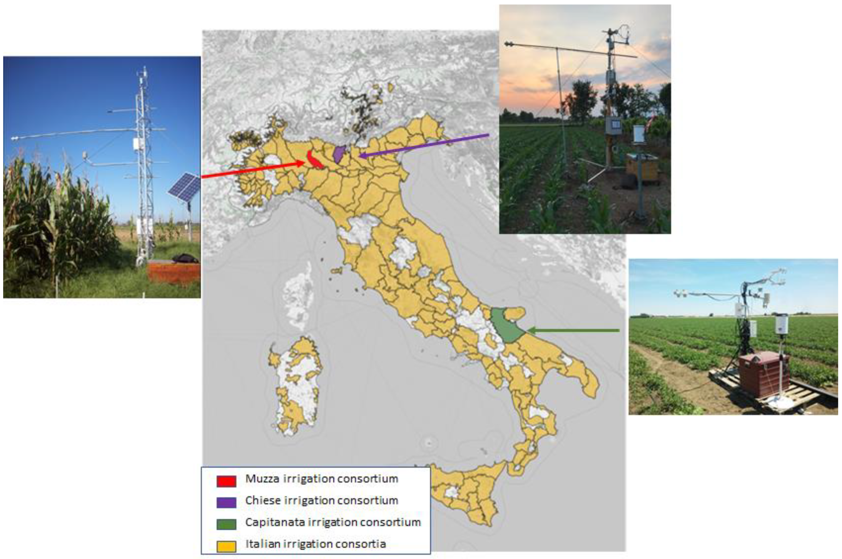
The analyzed case studies are several fields cultivated by tomatoes and maize across Italy, inserted in the Chiese, Muzza and Capitanata Irrigation Consortia (
Figure 1). These areas are selected because they are representative of the Italian agriculture in terms of crop types, irrigation schemes and water distribution rules, and they differ in climatic conditions, water volume availability and soil types among the same crop.
In all of the case studies, eddy covariance stations data are available (
Figure 1). These stations allow the measuring of the principal mass and energy fluxes, such as net radiation, evapotranspiration and heat sensible flux and soil moisture. Turbulent energy fluxes have been corrected, applying the whole range of correction procedures which are now well assessed in the scientific community [
41]. The data are analyzed with the PEC software (Polimi Eddy Covariance) [
42] which encompasses all the instrumental and physical corrections. [
42] compared corrected fluxes at high frequency data and at 30 min average data show that low errors can be obtained with mean absolute daily differences equal to 6.1 W m
−2 for H and 13.2 W m
−2 for LE.
2.1.1. Capitanata Irrigation Consortium (Southern Italy)
The Capitanata Irrigation Consortium (
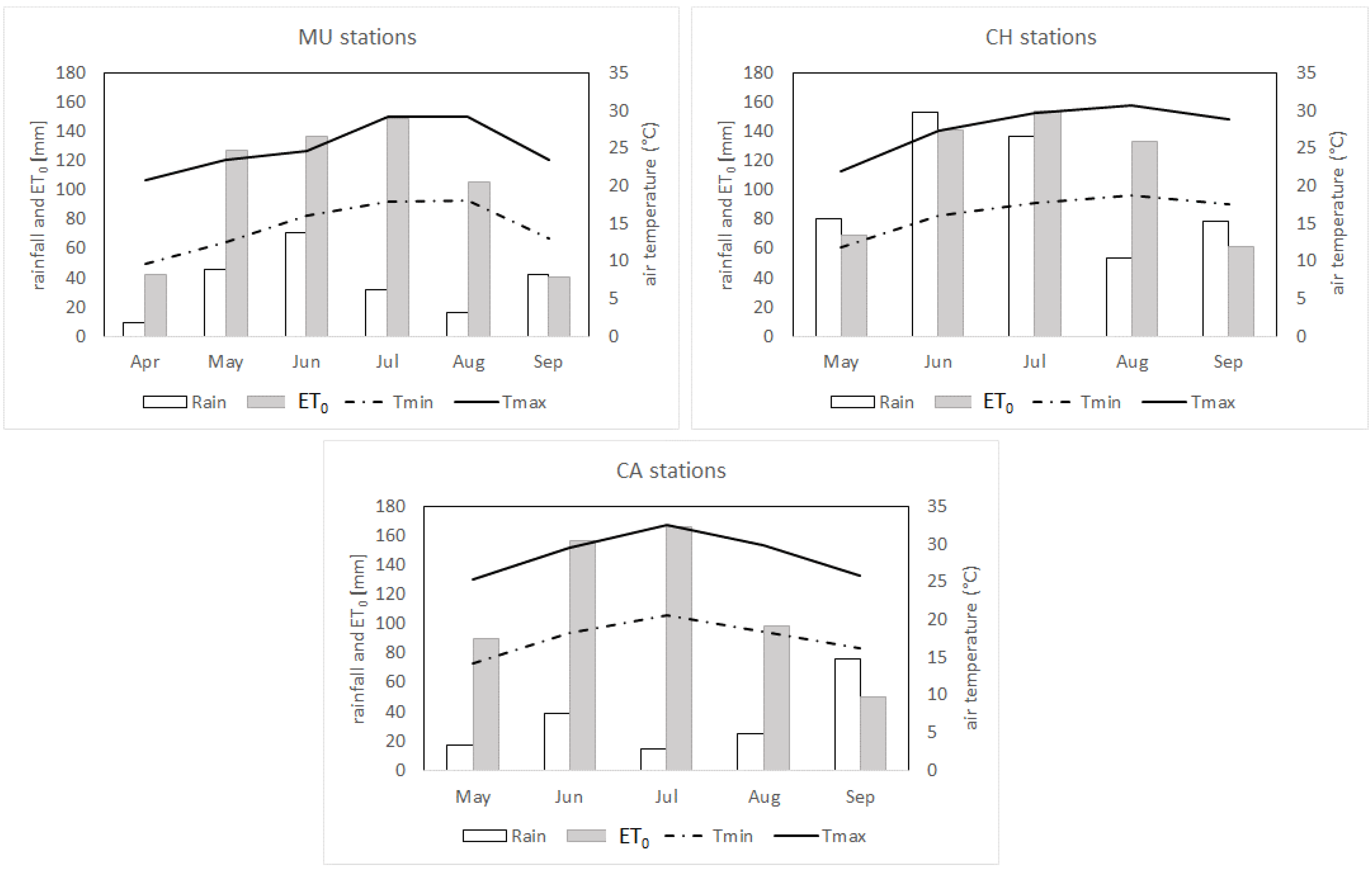
www.consorzio.fg.it, accessed on June 2015) is located in the Puglia region (Southern Italy), which is an intensive cultivation area mainly devoted to wheat, tomatoes and fresh vegetable cultivation with hot summers and warm winters. Irrigation water is supplied by a pressurized water network from storage dams’ reservoirs. The role of irrigation is crucial, with a mean volume of about 600 mm for the tomato fields, in the range of 5–35 mm per intervention at high frequency (one to three days between the interventions). The irrigation timing and volume are provided by the farmers. The most diffuse irrigation technique is drip irrigation, and water is available on demand. Rainfall during the crop season is about 160 mm, with an average daily mean temperature of 23.7 ± 2.8. The monthly total amounts of rain and ET
0 and the minimum and maximum air temperature monthly averages are 2.
Two eddy covariance stations are installed in tomato fields (
Table 1). Station 1 in field (CA1) was installed in May 2016 until October 2016 in a sandy soil field (
Figure 1), while Station 2 was installed in May 2016 until October 2016 in sandy soil field (CA2) [
43]. Soil moisture is measured with TDR (time domain reflectometer CS616, Campbell Sci, Logan, UT, USA) instruments at a 15 cm soil depth, which is representative of the tomatoes’ predominant rooting depths [
43] and at which the drip irrigation pipes system is installed. All the main meteorological variables (rainfall, air temperature and humidity, wind speed and radiation) are measured at an hourly time step.
The planting and sowing dates of the crops are reported in
Table 1.
2.1.2. Chiese Irrigation Consortium (Northern Italy)
The Chiese Irrigation Consortium (
www.consorziodibonificachiese.it, accessed on June 2015), down valley of the Lake Idro (Northern Italy), covers an area of 20,000 ha and is intensively cultivated with summer crops (i.e., corn, forage) and winter wheat, which cover about 68% and 8% of the agricultural land, respectively. The irrigation practice is based on fixed irrigation turns between every 7 ½ and 8 ½ days, which are defined a priori before the beginning of the irrigation season from April to September. The irrigation is provided to each field with a channel network of 1400 km covering an area of 18,000 ha. The irrigation is mainly flooding irrigation, with a fixed volume of 76 or 133 mm per each intervention, according to the irrigation schedule. Rainfall during the crop season is about 355 mm. The average of daily mean temperature throughout the growing season is 23.1 ± 3.8 °C. The monthly total amounts of rain and ET
0 and the minimum and maximum air temperature monthly averages are shown in
Figure 2.
An eddy covariance station has been installed in the same maize field between April and September in 2016 (CH1), in 2017 (CH2) and in 2018 (CH3) (
Table 1) [
36]. Soil moisture is measured with TDR instruments (CS616, Campbell Sci, Logan, UT, USA) at 35 cm soil depth, which is representative of the maize maximum density of roots [
44]. All the main meteorological variables (rainfall, air temperature and humidity, wind speed and radiation) are measured at an hourly time step.
The planting and sowing dates of the crops are reported in
Table 1.
According to ISTAT, for Brescia province, the production is equal to 12.5 ton/ha of maize grains (
http://dati.istat.it/, accessed on 15 June 2020).
2.1.3. Muzza Irrigation Consortium (Northern Italy)
The Muzza Bassa Lodigiana irrigation consortium is located in the middle of the Po Valley (Northern Italy), with an area of 740 km
2 which is divided into over 150 irrigation basins. The Muzza canal, the largest irrigation canal in Italy, derives water from the Adda river. Average annual rainfall in the consortium ranges between 800 (southern area) and 1000 mm (northern area) with two peaks in spring and autumn. Flood irrigation is scheduled by the consortium so that farmers can irrigate once every 2 weeks. In the period 2010–2012, an eddy covariance station was installed in the same maize field in Livraga town (MU1-MU2-MU3), characterized by a clay loam soil [
45]. Soil moisture is measured with TDR instruments (CS616, Campbell Sci, Logan, UT, USA) at a 35 cm soil depth, which is representative of the maximum density of roots (Lundstrom, 1988). All the main meteorological variables (rainfall, air temperature and humidity, wind speed and radiation) are measured at an hourly time step. The monthly total amounts of rain and ET
0 and the minimum and maximum air temperature monthly averages are shown in
Figure 2.
The planting and sowing dates of the crops are reported in
Table 1.
2.1.4. Remote Sensing Data
For the Capitanata Irrigation Consortium case study, vegetation indices are obtained from Sentinel-2 and Landsat8 data at a high spatial resolution (30 m) which is suitable to correctly follow the fields’ dimension [
43,
46]. The vegetation fraction (CC) is computed as:
where NDVIs and NDVIv are representative NDVI values for bare areas (0.15) and green vegetation (0.9), respectively. LAI is then calculated as:
Here, k(θ) is the light extinction coefficient for a given solar zenith angle. The solar zenith angle (θ) depends on terrain geometry, solar declination, solar elevation angle, latitudinal location and day of the year. The light extinction coefficient is a measure of attenuation of radiation in the canopy, usually equal to 0.5.
The MODIS sensor on board the operative satellites Terra and Aqua is used to retrieved vegetation parameters (
https://lpdaac.usgs.gov/, accessed on 15 January 2020). Leaf area index (LAI), defined as one-sided green leaf area per unit ground area, was retrieved from the MODIS LAI products (MOD15A2–leaf area index) generated over an 8-day compositing period with a spatial resolution of 1 km. MODIS data are used for the Northern Italy case studies, where a low spatial resolution has been proved to be able to correctly reproduce the vegetation dynamic of the area due to its homogeneity [
45].
2.2. The AquaCrop Model and Water Efficiency Indicators
AquaCrop (
http://www.fao.org/nr/water/aquacrop.html, accessed on 15 March 2018) is an agronomic model for crop production and irrigation water needs optimization, which has been developed by the Land and Water Division of FAO [
5].
Canopy cover (CC), biomass (B) and Yyields (Y) of a crop are the main model variables which are computed as a function of water productivity, i.e., the biomass produced per unit of water transpired by the vegetation under the present climate conditions [
47]. Stress coefficients which account for available water, air temperature, soil fertility and salinity may reduce the final crop productivity as they influence the canopy expansion processes, stomata control of transpiration, canopy senescence and Harvest Index (HI).
The AquaCrop model solves a complete water balance, where crop evapotranspiration is computed according to the crop coefficient of each crop [
23] multiplied by the reference evapotranspiration ET
0 [
48] and its a function of CC. HI, along with CC, determines the amount of produced biomass (B) and yield (Y) [
6]. Cumulative biomass production is obtained as the sum of the daily ratio between crop transpiration and ET
0 for each day of the crop cycle, and the crop yield is calculated by multiplying the final biomass by a specific crop HI. The coefficient of transformation between dry biomass and fresh yield is set as equal to 0.055 for tomatoes [
49].
A detailed description of the AquaCrop model may be found in [
5,
47].
In this paper, meteorological variables measured at the fields’ sites, such as the minimum and maximum air temperatures, wind speed, air humidity and incoming solar radiation, are used to estimate ET0. Measured rainfall and irrigation are also used as input data. The initial soil moisture condition for each field is set equal as to the observed value at the time of the initialization.
The AquaCrop model is based on several parameters for crop, soil and environmental calculations. Some of these parameters have been proved to remain almost constant over the computation time [
47], while others need a specific calibration. In this paper, the calibration of soil hydraulic and crop parameters is performed through the comparison between estimated and observed ground soil moisture and satellite LAI and CC. The model is then validated against ground measurements of evapotranspiration and crop yield. The model is run with different parameters configurations and with a trial and error approach; the parameters are modified from the original values minimizing the difference between observed and simulated variables. The soil parameters are set according to [
50], assigning to each field of the analysed area its respective value. The parameters values are modified, keeping their values in their physical ranges. The main considered soil parameters are: ksat as saturated hydraulic conductivity, fc as field capacity, wp as wilting point, SMsat as soil moisture value at saturation, CN as curve number. Another important parameter to be defined is soil depth, considered the predominant growing zone of fresh vegetable roots, relevant for the evapotranspiration process. The crop parameters are set as the standard values from AquaCrop and then calibrated.In
Table 2, the values of the main soil parameters which have been calibrated are shown for each field, while in
Table 3 the crop parameters are reported for the two crops (maize and tomatoes).
2.2.1. The Optimized Irrigation Strategy
The optimized irrigation strategy [
36,
37] allows one to keep the present and forecasted soil moisture between two soil moisture thresholds: the higher one relative to soil moisture content for which the percolation flux in the soil starts to be significant (field capacity) and a lower one where the crop begins to suffer for lack of soil water (crop stress). This criterion supports the correct timing of irrigation and the amount of water for each irrigation, allowing one to reduce the passages over the field capacity threshold reducing the percolation flux with a saving of irrigation volume, while evapotranspiration remains almost the same. The optimized irrigation strategy allows one to increase the irrigation efficiency (ton/mc) and water productivity (€/mc), saving an important percentage of water, but also of fertilizer and energy, as compared to today’s irrigation practices.
The decision criteria for planning whether or not to irrigate are based on the comparison between the soil moisture and a water stress threshold (θcrit), below which the crop begins to suffer for lack of water. This criterion will determine the correct timing of irrigation and the amount of water.
This stress threshold is a function of the different types of soils and crops, but also of the vegetation growth stage and of the climatology of the area of study. The implemented procedure relies on a θ
crit which is computed following the methodology of [
23] based on:
where RAW is the readily available water, defined as field capacity minus stress threshold; TAW is the total available water, defined as field capacity minus wilting point; and p is a reduction coefficient depending on the crop and climatic parameters. p is defined by [
23] for several crops, which is then corrected for climatic data. The factor p normally varies from 0.30 for shallow-rooted plants at high rates of ETc (>8 mm d
−1) to 0.70 for deep-rooted plants at low rates of ETc (<3 mm d
−1). The p coefficient tabulated according to [
23] applies for ET of about 5 mm/day. The value for p is adjusted for different ET according to
where ET is mm/day.
Then, θ
cit is computed to be equal:
A surplus threshold can also be identified equal to the field capacity of the soil.
2.2.2. Water Efficiency Indicators
A series of water indicators are computed for the summarized the effect of irrigation optimization of yield production and water use, but also for the general impact on water fluxes (e.g., drainage flux). These are computed as:
Water use efficiency [ton/m
3]:
Irrigation water use efficiency [ton/m
3]:
Irrigation efficiency:
where yield is the crop yield (ton ha
−1), ETm is the evapotranspiration (m
3 ha
−1), Im is the observed or modelled irrigation volume (m
3 ha
−1), P is rainfall (mm), I is irrigation (mm), Perc is the drainage flux (mm) and ET is the evapotranspiration (mm).
2.2.3. Evaluation of the Model’s Performance
The reliability of the different estimates will be evaluated using different statistical indexes which are the absolute mean error (MAE), the root mean square error (RMSE), the modelling efficiency index (EI) and the average relative error (ARE), computed as follows:
where P
i is the ith simulated variable, O
i is the ith measured variable, n the sample size and
the average observed variable. EI can range from −∞ to 1, and the closer the model efficiency is to 1, the more accurate the model is, while for MAE, RMSE and ARE, the best value is 0.
3. Results
3.1. Model Calibration
3.1.1. Tomato Fields: Capitanata Irrigation Consortium
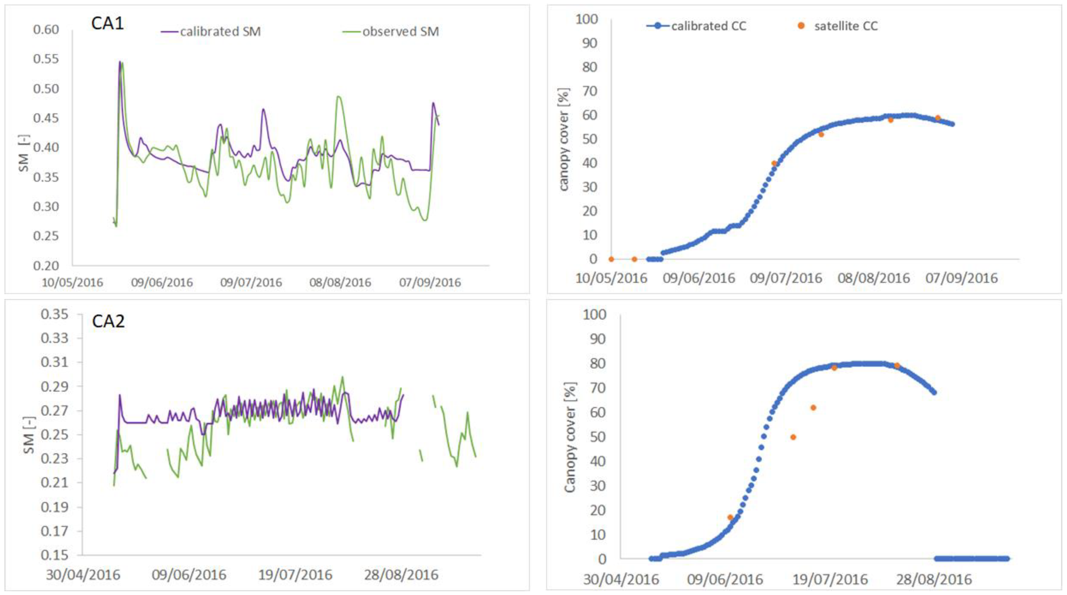
The AquaCrop model is calibrated for the two tomato fields using the observed irrigations as provided by the farmers. In the first field (CA1), soil moisture is sensibly underestimated before calibration with a negative EI (−0.78) and an MAE of 0.045, while after the calibration a good agreement is found with an EI of 0.48 and an MAE of 0.026. In
Figure 3, the soil moisture series after the calibration are reported against observed data, showing the goodness of the model after the calibration procedure. Evapotranspiration is simulated with an MAE of 0.6 mm/day with the calibrated parameters.
The simulated fresh yield is then compared to the observed one, showing a good agreement after all the calibration process with an observed yield of 110 ton ha
−1 and a simulated one of 99.8 ton ha
−1, leading to an error of 9%. Canopy cover has then been compared with Landsat8 data, and a good agreement is observable with a relative error of 1%. In
Table 4, the statistical indices RMSE and MAE are reported after the calibration procedure showing good agreement between observed and simulated variables.
Good performances are also obtained for the second tomato field (CA2), showing a clear improvement before and after the calibration process. This is confirmed by the statistical indices with an MAE of soil moisture that ranges from 0.084 to 0.015 and an EI from −0.15 to 0.24, while an MAE of 0.4 mm/day is found for ET. The error of yield is less than 1% with a modelled value at the end of the season of 111.1 ton/ha and an observed one of 110 ton/ha. The error of canopy cover estimates with respect to satellite data is equal to 4%.
3.1.2. Maize Fields: Chiese and Muzza Irrigation Consortia
The results from these two irrigation consortia are presented together due to the fact that in both analysed fields, the cultivated crop is maize with a similar climate, but the soil composition is very different with sandy soil in the Calcinato field and clay loam in the Livraga field.
Chiese Irrigation Consortium
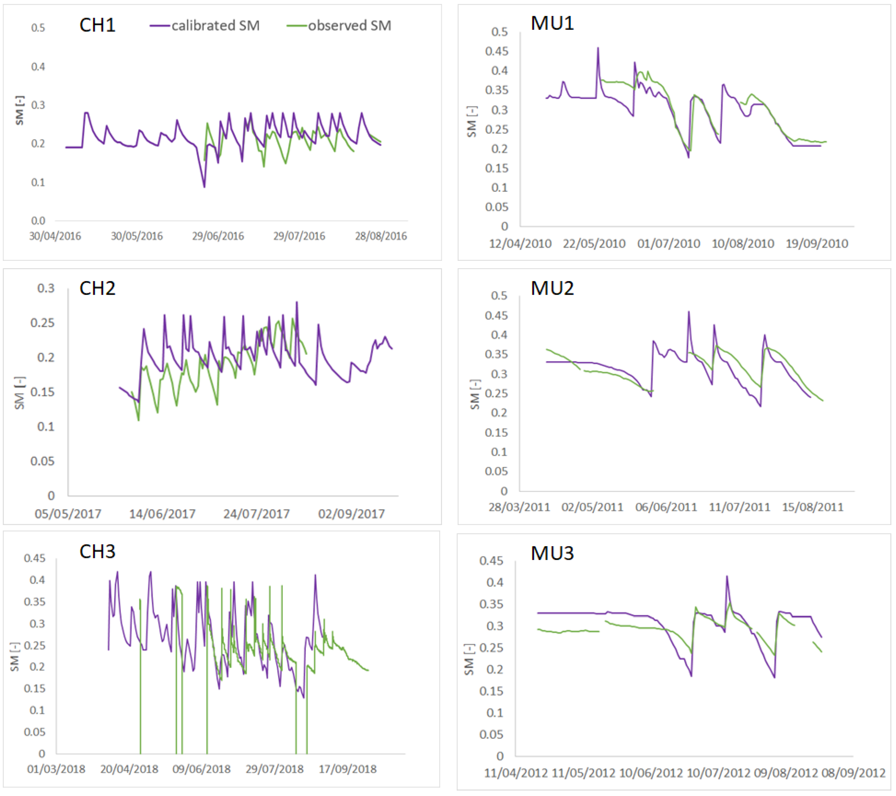
The model is calibrated for the year 2016 and then validated during 2017 and 2018, the station being installed in the same field. A clear improvement is obtained after the calibration process in the 2016 crop season (
Table 5), with an MAE of soil moisture which reaches 0.03 and an MAE of 0.6 mm/day on ET. In
Figure 4, the soil moisture series after calibration are reported against the observed data, showing their good agreement for either low or high values.
The error of yield is less than 2 ton/ha, while an MAE and an RMSE of 1.3 and 0.4%, respectively, are obtained for canopy cover. The ability of the model to reproduce the temporal dynamic of crop grow coverage is shown in
Figure 5 against the satellite data. During the validation phase, a high accuracy is also obtained for 2017 soil moisture estimates, with an MAE of 0.021 and an RMSE of 0.4 (
Figure 4), while the production is slightly less than the observed one, with an error of 1 ton/ha. An error of 1.5 ton/ha is obtained for 2018. The canopy cover dynamic is well reproduced (
Figure 5) both in 2017 and 2018, with an MAE of 3.6 and 7%, respectively. Evapotranspiration is also well simulated, with an MAE of 0.4 mm/day during the 2017 crop season and 0.3 mm/day during 2018.
Muzza Irrigation Consortium
The model is calibrated for the Muzza maize fields in the year 2010 and then validated during 2011 and 2012, the station being installed in the same field. During the 2010 growing season, soil moisture values are simulated with good accuracy, with an MAE of 0.02 and a similar RMSE.
Figure 4 shows the comparison between observed and simulated soil after the calibration process. Evapotranspiration shows also an agreement with observed data, with an MAE of 0.97 mm/day and an RMSE of 1.2 mm/day (
Table 5). The fresh crop yield is equal to 14.6 ton/ha, which slightly overestimates the observed statistical values of 21%. A higher accuracy is obtained for canopy cover, with the model and the remote sensing data differing by 4% (
Figure 5).
Similar results are obtained during the validation periods, the MAE of soil moisture being 0.02 for both 2011 and 2012 (
Figure 4), and the MAE of ET 1 mm/day and 0.93 mm/day for 2011 and 2012, respectively. During the 2011 crop season, the maize yield reaches 11.88 ton/ha of fresh products, which is 0.9% less than the observed statistical values, while during 2012 similar yield values are obtained (11.2 ton/ha) with an error of 6.2% in respect to observed data. Differences of the modeled and remotely observed canopy cover are found to be 3.5 and 5% during 2011 and 2012, respectively.
3.2. The Optimized Irrigation Strategy
The optimization irrigation strategy is then applied to all the analyzed fields in the different crops’ seasons evaluating the effect not only on irrigation volumes and number of irrigations, but also on crop yield and on the total cumulated drainage flux which represents the main water loss (e.g., not used by the plants to grow).
3.2.1. Tomato Fields: Capitanata Irrigation Consortium
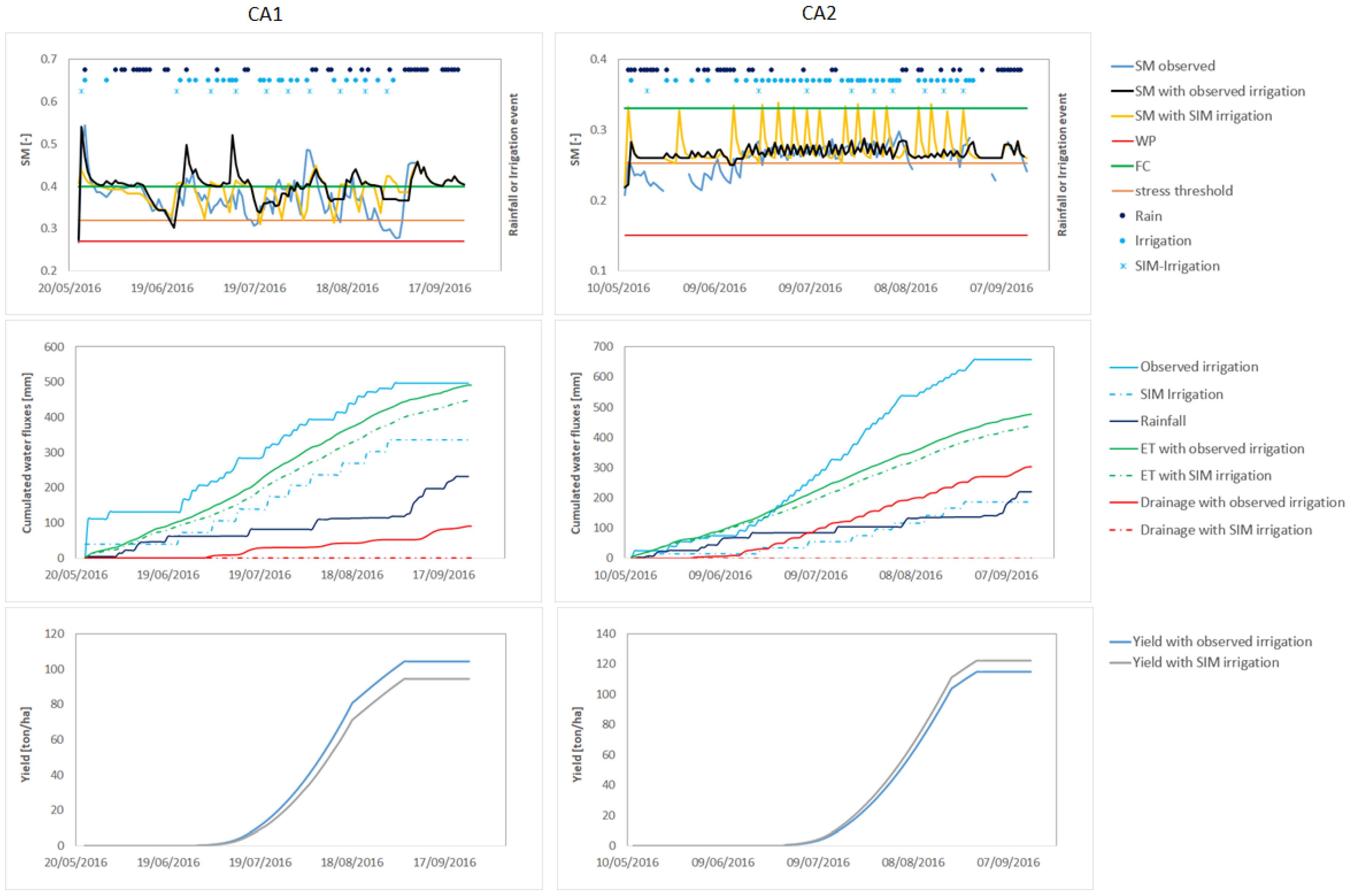
In
Figure 6, the results of the SIM irrigation strategy are shown for the tomato fields. Two simulations are compared: “SM with observed irrigation” (e.g., using as input data the irrigations provided by the farmers) and the “SM with SIM irrigation” (e.g., triggering the irrigation when the stress threshold is reached). The two simulations are then compared with the measured SM in each field. For CA1, the differences in soil moisture behaviour between the modelled values with observed and SIM irrigations are clearly visible between the two lines showing the different strategy ideas, especially on the high peaks and the irrigation timing. This is reflected in the reduction in the irrigation volume by 37.6%: the observed one is equal to 516 mm, while the SIM one is equal to 322 mm (
Table 6). A decrease in the irrigation events by 15 is also observable between the two strategies.
Then, a considerable difference is also observable when all the modelled water balance fluxes are compared when using the two different irrigation strategies (
Figure 6). In particular, with the SIM irrigation, the percolation flux is sensibly reduced, allowing the saving of a considerable amount of water, while evapotranspiration remains almost the same, as expected. The yield with the SIM strategy is slightly reduced to 92.9 ton/ha with a loss of 7% of productivity.
For field CA2, using the SIM strategy the irrigation water volume would go from 644 mm to 590 mm with a saving of 8.7%, which would lead to a production gain of 2.7% (yield with SIM strategy equal to 113.2 ton/ha). Similar to CA1, ET remains almost similar between the two irrigation strategies, while a significant improvement is observable in the reduction in the drainage flux with the SIM strategy by about 50 mm.
Comparing the two tomato fields, the irrigation volume reduction with the implementation of the SIM strategy for CA2 is lower than for CA1, due to the different soil types of the two fields (
Table 1). In fact, CA2 field has a sandy soil with a higher infiltration capacity (higher hydraulic conductivity) as compared to the silty clay soil of field CA2. However, the reduction in irrigation events is higher (27) in CA2 than in CA1 (15), which may be also as important as the irrigation volume reduction, especially in terms of economic savings (e.g., electricity, labour).
3.2.2. Maize Fields: Chiese and Muzza Irrigation Consortia
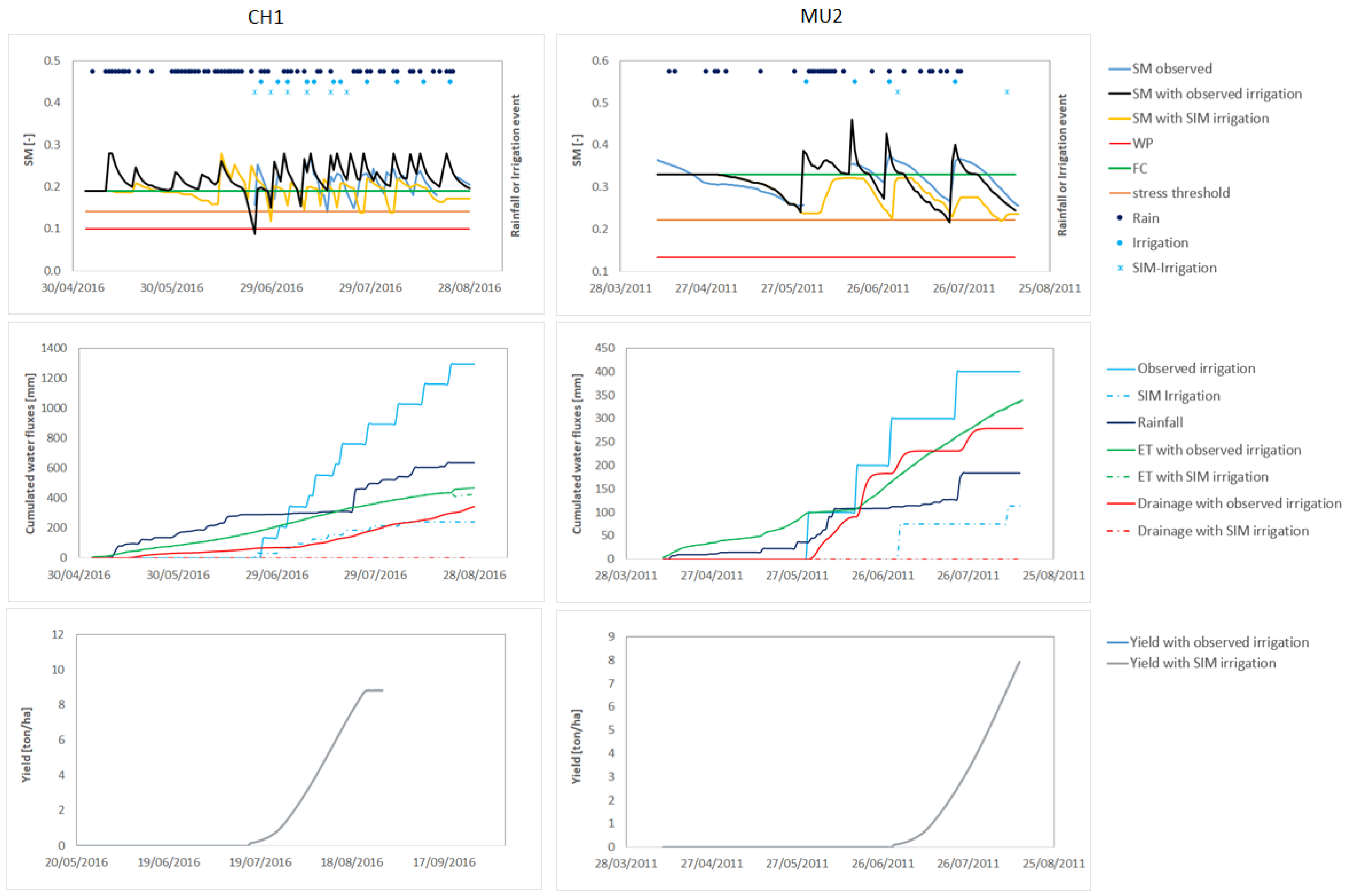
For the Chiese consortium, if the SIM strategy is applied to field CH1, the irrigation water volume saved would have been of about 1000 mm which could lead to a significant reduction in the drainage flux by about 200 mm and in the runoff flux by the remaining 800 m, while the evaporation flux remains almost constant. This last one is one of the main reasons for an unchanged production between the two irrigation strategies, which is around 9 ton/ha. Soil moisture behaviour is modified when applying the SIM strategy (
Figure 7), and it is especially visible in the SM peaks which do not surpass the FC value.
For CH2, similar results are obtained when the SIM irrigation strategy is applied, showing a difference on soil moisture behaviour, especially on the high peaks and in the irrigation timing. The reduction in the irrigation volume between the observed and SIM strategies (
Table 7) would be remarkable and equal to more than 1000 mm together with a reduction of 8 irrigation events. As expected also during 2017, a considerable difference is observable in the percolation flux which is reduced by 200 mm in addition to the runoff by about 800 mm. The yield, in this case, is sensibly increased from 7 to 9 ton/ha due to the excess of water provided with the observed irrigation strategy, which leads to SM values almost always above the FC.
The same results (
Table 7) are also obtained for CH3 during the 2018 crop season, where the implementation of the SIM strategy would lead to a similar reduction in the irrigation volume (about 1000 mm less) and number of irrigation events, as well as in the drainage flux. A similar crop yield is also obtained between the two irrigation strategies, confirming the optimization of the SIM one.
It is interesting to note that during the different crop seasons from 2006 to 2008 in the maize field of the Chiese Irrigation Consoritum, the same irrigation volume has been provided even though significantly different rainfall volumes are observed (from 200 to 600 mm). The SIM strategy allows the sensible improvement of the irrigation volume, considering also the rainfall as a water balance input.
For MU fields in the Muzza Irrigation Consortium, the same analysis is performed. In general, the modeled soil moisture with the observed irrigations has a similar behavior to that obtained by applying the SIM strategy, except for the peaks where the SM with observed irrigations far surpasses the FC threshold (
Figure 7). This would lead to a mean reduction by 150 mm of the percolation flux with SIM irrigations, compared to the one computed with observed irrigations. This is related to the reduction in irrigation volume which is visible during the three analysed years. For MU1, the observed irrigation volume is equal to 400 mm, while the SIM one is equal to 240 mm, with a reduction of 40% (
Table 7). One irrigation event less is also obtained with the SIM strategy. The evapotranspiration flux remains almost the same when applying the two irrigation strategies. A similar behaviour is observed for crop yield. For field MU2, the highest reduction in irrigation water volumes is observable from 400 mm to 113 mm if the SIM strategy is applied. The same yield production is kept, as well as ET. Similar to MU1 and also MU3, the irrigation volume is slightly reduced and ET remains almost similar between the two irrigation strategies, as well as the yield.
Comparing the two maize fields in the Muzza and Chiese Irrigation Consortia, the differences are clearly visible between the two sites of the effect of the SIM strategy application on irrigation water saving, water fluxes and crop yield production. In fact, irrigation volume reduction with the SIM strategy for MU is significantly lower than for CH fields (70% and 40%, respectively), which is mainly due to the different soil types of the two areas (
Table 1) for a similar rainfall. In fact, the MU field has a sandy soil with a higher infiltration capacity than the silty clay soil of the CH field. This is reflected mainly in the reduction in water losses for percolation. Moreover, usually in the Chiese Consortium 13 irrigations are performed while only four are in the Muzza Consortium, which may also be as important as the irrigation volume reduction in terms of economic savings (e.g., electricity, labour).
3.2.3. Stress Threshold Sensitivity Analysis
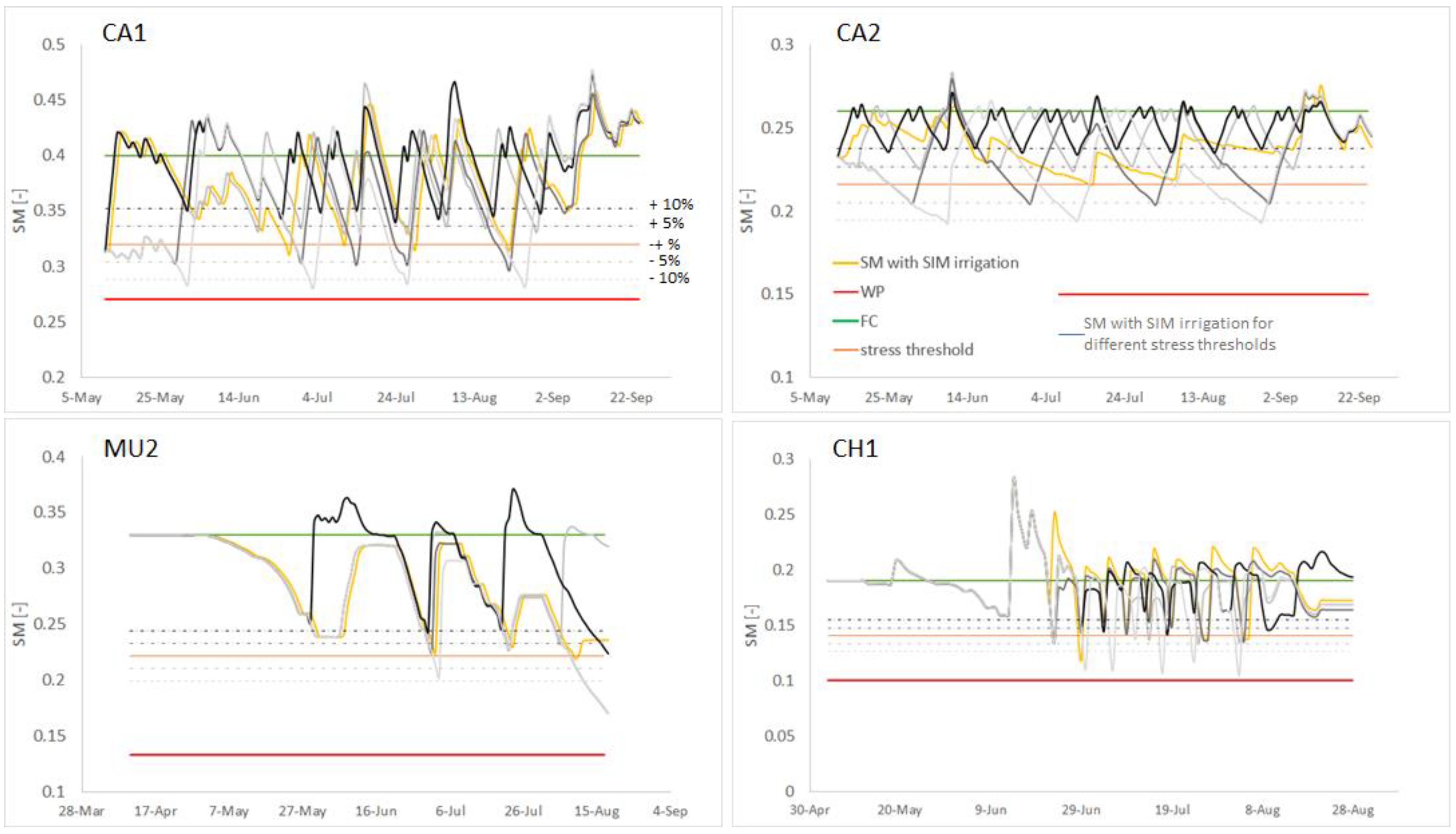
The evaluation of the sensitivity to the stress threshold is performed applying the SIM irrigation strategy with the fixed calibrated parameters for each field, then the p value is changed to between +10% and −10% in steps of 5%. The results of the sensitivity analysis to this stress parameter are provided in
Figure 8 in respect to soil moisture for the two tomato fields (CA1 and CA2) and for two maize fields (MU2 and CH1). The yellow line represents the simulated value with the SIM strategy with the original p value from [
23], while the additional simulations, obtained by varying the p values, are represented in a gray color scale. The uncertainties linked to p considerably affect the soil moisture behavior and hence the irrigation triggering timing.
Table 8 represents the effect of soil moisture stress threshold on total irrigation volume used in the two farms. The effect is shown in percentage of change; as expected, a considerable volume increase is obtained with a higher stress threshold and a volume decrease with a lower stress threshold.
These changes are directly reflected in crop yield and hence crop productivity. In
Table 8, the total yields (ton/ha) are finally compared at varying the stress thresholds, and as expected, the values remain almost constant. In general, a similar production to the original p value is found if the stress threshold is increased by 5 and 10% which, however, corresponds to higher irrigation volumes. Slightly lower crop yields (1%) are obtained with the decrease in the stress threshold, which correspond to a considerable decrease in the irrigation volume (5–15%). Similar results are obtained for the different crops and the different soil types (
Table 1), suggesting that for these case studies the values identified by [
23] are suitable, while a high importance of the p value definition is of extreme importance in water saving analysis.
3.3. Water Efficiency Indicators
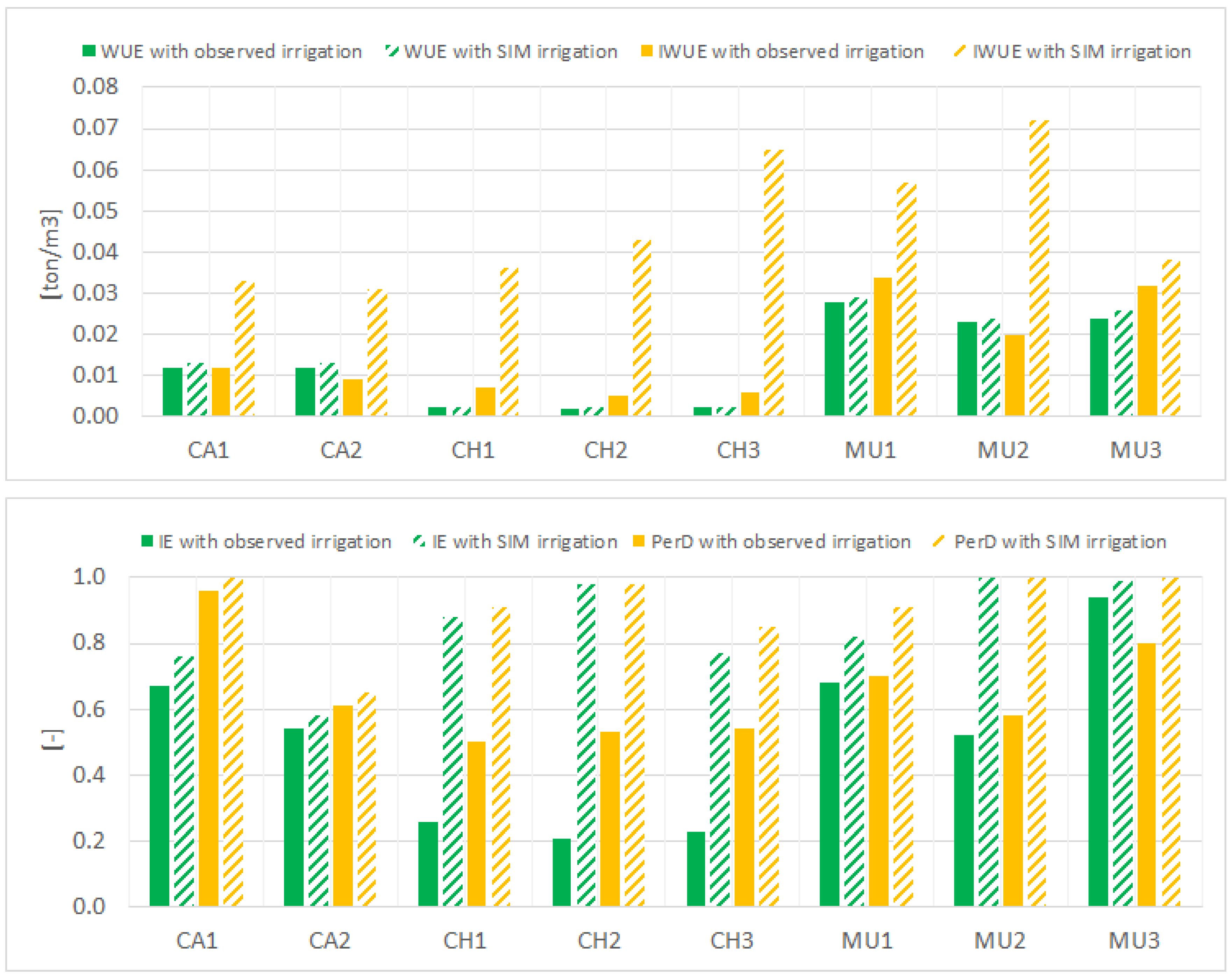
The optimization irrigation strategy has been applied to all the analyzed fields in the different crops seasons evaluating the effect not only on irrigation volumes and number of irrigations, but also on crop yield and canopy cover, and on the cumulated drainage flux which represents the main water loss (e.g., not used by the plants to grow). To summarize the effect of the SIM irrigation strategy and to quantify its efficiency, a series of water indicators is computed (
Figure 9).
In general, the SIM strategy leads to higher IWUE than with the observed irrigations, and also to a higher percolation deficit and irrigation efficiency confirming the SIM strategy objective and potentiality, keeping constant the WUE indicators (e.g., almost unchanged crop yield and evapotranspiration).
The highest improvements of IWUE (around 0.04 ton/m3) are obtained for the two irrigation consortia in Northern Italy, where high amounts of irrigation water are traditionally used in excess, which the SIM strategy may help in reducing. The amount of used irrigation water is quite similar every year, but with significantly different rainfall volumes. This results from the ancient water rate concessions where water is paid at a fixed amount per year, and not as the real used water.
In any case, even in the Capitanata area generally characterized by less water availability which over the years has led farmers to pay greater attention to the use of irrigation water, improvement of IWUE may be obtained following the SIM strategy (around 0.02 ton/m3).
The IE index, following the IWUE behavior, shows a great improvement in the two Northern Italy consortia when the SIM methodology is implemented (about 0.7 in the Chiese area and 0.3 in the Muzza area).
In general, the PerD index tends to 1 in the case where the deep percolation flux is null, a situation which may be reached by applying the SIM strategy. This is reached in most of the situations, except in field CA2 which, as previously noted, is characterized by a high permeable soil leading to minimum water loss even when applying the SIM strategy.
4. Discussion
In this paper, the effect of the SIM optimization irrigation strategy based on crop stress thresholds has been implemented, showing the possibility of enhancing the actual irrigation practices in real applications across two Italian irrigation consortia for tomato and maize fields which differ in climate, soil types and irrigation technique. This can lead not only to a reduction in irrigation volumes and number of irrigations, but also in the drainage flux which represents the main water loss, keeping the crop yield and canopy cover constant.
SIM is an often used approach in irrigated cropping systems, especially those where precision irrigation is carried out. It is an effective system in cases where the capillary rise is negligible and irrigation rates are not excessive, if applied on soils with good drainage. However, this is not the case in the presented cases studies, where the analyses confirm the significantly high amounts of water used for irrigation which can be reduced even in areas where efficient irrigation management is used (e.g., the Capitanata area). The results are even more relevant for Northern Italy in the case studies of Chiese and Muzza characterized by a high waste of water with inefficient irrigation techniques.
The performed analysis relies on a calibrated AquaCrop model which has been able to correctly reproduce the crop yield and also other output variables such as ET, SM and CC. In fact, some previous studies calibrated the AquaCrop model only on crop yield, assuming then that the model was able to correctly reproduce also soil moisture or evapotranspiration [
10,
49,
51]. However, this is not always verified as reported by [
52], who showed differences in performances depending on crop types, water stress and output variables (ET, SM, yield, CC). For example, [
52] reported ET underestimation when maize and tomatoes are stressed, while [
53] found a better ET agreement for cotton under water stress than not stressed. Moreover, the AquaCrop ET computation methodology based on ET
0 and Kc has been criticized for its application, especially in the Mediterranean area [
54,
55]. The correctness of all output variables is of extreme importance when the AquaCrop model is used as a tool for irrigation scheduling based on daily ET [
53,
54,
56], SM [
57] or IWUE [
28].
Moreover, several studies on irrigation management did not compute water efficiency indicators as WUE or IWUE [
58,
59,
60].
The results obtained in this paper in terms of IWUE are in line with literature values. In fact, for example [
61] found that for tomatoes, the IWUE ranges from 0.357 to 0.876 kg/m
3 for the different irrigation water levels, with IWUE increasing with irrigation volume. They also reported a saving up to 35% of tomato irrigation volume without significant reduction in fruit yield. This confirming also the findings of [
62]. The study in [
63] found that the IWUE of tomatoes can be significantly reduced with less irrigation water volume. For maize fields, [
64] found that decreasing irrigation volume of 10% maintained similar grain yield, while decreasing evapotranspiration and increasing WUE (4.61–6.66%). The study in [
65] found that in the middle Heihe river basin, a reduction of 23% of irrigation water did not reduce yield.
Nevertheless, the comparison of WUE among different locations is challenging due to the different climatic conditions, water and soil management [
35].
Another point of discussion may be related to the annulment of the percolation flux, which may cause a problem for some soils characterized by a high salt or fertilizer concentration [
40,
66], which need a more comprehensive control of irrigation.
Finally, the importance of the p value definition is of extreme importance in water saving analyses, which can lead to a significant variation in irrigation volumes. The definition of a variable stress threshold during the crop growing can better allow a more precise irrigation triggering.
5. Conclusions
In this paper, the AquaCrop model has been used for optimizing the irrigation water use efficiency for tomato and maize fields across Italy, based on the operative SIM strategy which accounts for crop stress thresholds evaluating the effect not only on irrigation volumes and number of irrigations but also on crop yield and canopy cover, and on the cumulated drainage flux which represents the main water loss (e.g., not used by the plants to grow). The results provide irrigation management suggestions for a single farmer who seems to use too much water, but also for consortia to review their management among the associated farmers.
In fact, irrigation volume reductions are found to be between 200 and 1000 mm when applying the SIM strategy, mainly depending on the different soil types more than on the climate, irrigation technique or crop. This is directly related to the drainage flux reduction which is of a similar entity.
The SIM strategy efficiency has then been summarized by different indicators: the IWUE, which is higher than with the observed irrigations (around 35% for tomato fields in Southern Italy and between 30 and 80% for maize in Northern Italy), and also a higher percolation deficit and irrigation efficiency confirming the SIM strategy objective and potentiality.
The AquaCrop model has been previously calibrated against canopy cover and LAI from remote sensing data, producing MAE errors between 1 and 15%, while MAE between 0.015 and 0.04 are obtained for SM. The validation of the AquaCrop model has been performed against ET ground-measured data and crop yields, producing MAE values ranging from 0.3 to 0.9 mm/day, and 0.9 ton/ha for maize and 10 ton/ha for tomatoes, respectively.


