Alteration of the Ecohydrological Status of the Intermittent Flow Rivers and Ephemeral Streams due to the Climate Change Impact (Case Study: Tsiknias River)

Abstract

Climate change projections predict the increase of no-rain periods and storm intensity resulting in high hydrologic alteration of the Mediterranean rivers. Intermittent flow Rivers and Ephemeral Streams (IRES) are particularly vulnerable to spatiotemporal variation of climate variables, land use changes and other anthropogenic factors. In this work, the impact of climate change on the aquatic state of IRES is assessed by the combination of the hydrological model Soil and Water Assessment Tool (SWAT) and the Temporary Rivers Ecological and Hydrological Status (TREHS) tool under two different Representative Concentration Pathways (RCP 4.5 and RCP 8.5) using CORDEX model simulations. A significant decrease of 20–40% of the annual flow of the examined river (Tsiknias River, Greece) is predicted during the next 100 years with an increase in the frequency of extreme flood events as captured with almost all Regional Climate Models (RCMs) simulations. The occurrence patterns of hyporheic and edaphic aquatic states show a temporal extension of these states through the whole year due to the elongation of the dry period. A shift to the Intermittent-Pools regime type shows dominance according to numerous climate change scenarios, harming, as a consequence, both the ecological system and the social-economic one.

1. Introduction

The water framework directive (WFD) established an integrated approach on management and protection of Europe’s aquatic environment and set the general goals to achieve a “good water status” for European water bodies [1]. These goals, however, seemed more directed towards permanent rivers, neglecting the important contribution of intermittent streams; these are defined as all temporary, ephemeral, seasonal, and episodic streams and rivers in defined channels, in which flow is interrupted either spatially or in time [2]. Ecosystem services provided by IRES are strongly affected by their hydrological phases, with dry phase having potentially negative impact on several services and especially agricultural production [3].

Temporary streams constitute more than 50% of the global network, and this number is growing due to climate change; the status of the majority of rivers is switching from perennial to intermittent [4]. According to the Fifth Assessment Report (AR5) of the Intergovernmental Panel on Climate Change (IPCC), surface temperature is projected to rise over the 21 century under all assessed emission scenarios, while precipitation trends will not be uniform over the Earth’s different regions [5]. It is very likely that heat waves will occur more often and last longer and that extreme precipitation events will become more intense and frequent, particularly in the Mediterranean area [5,6,7]. For instance, large-scale predictions for Mediterranean suggest up to 35% rainfall reduction and 3–5 °C temperature increase by 2071–2100 [8,9]. A climate change impact study conducted at basin scale in Portugal under RCP 4.5 and RCP 8.5 scenarios, comparing past (1950–2015) and future (2021–2100) climate, reached some concerning conclusions: annual temperatures are expected to increase by 10–20%, precipitation will decrease by 8–13%, and river flow will decrease by 28% [10]. Furthermore, based on the international Coordinated Regional Downscaling Experiment (CORDEX) simulations, the CORDEX ensemble corroborates the fact that the Mediterranean is already entering the 1.5 °C climate warming era. The southern part of the Mediterranean is expected to be impacted most strongly since the CORDEX ensemble suggests substantial combined warming and drying, particularly for pathways RCP 4.5 and RCP 8.5 [11]. Climate change will exacerbate the problems of water scarcity that will be more pronounced during the dry season; the transition from perennial to intermittent status for many rivers due to CC coupled with the effect of anthropogenic pressures on water resources will affect their ecological status [12,13].

All the above indicate the importance of the hydrological status of rivers and temporary streams in particular. The latter are less integrated in regional and global analysis, water legislation, and regulations because of the difficulties they display when compared to permanent rivers [14], especially in the ecological aspect of the assessment. The shifting lotic, lentic, and terrestrial habitats are unique in spatial arrangement and connectivity. They are controlled mainly by the magnitude, frequency, and duration of drying spells in these systems [4]. The increase, however, in fragmentation of rivers networks results in dispersal-limited freshwater ecosystems influencing the metacommunity dynamics [15]. In this perspective, the biodiversity and several ecosystem services are vulnerable to the river intermittency especially under climate change. These habitats are threatened with extinction by the projected climate change impacts.

In recent years, several initiatives and projects have been launched especially in the Mediterranean region, resulting in the introduction of new tools such as the TREHS tool for temporary rivers [16]. No studies have been conducted thus far using the TREHS tool (outside of the EU LIFE TRIVERS project), utilizing its capacity to assess the hydrological regime of temporary rivers. TREHS is used to classify the intermittent streams regime and status/degree of alteration based on metrics from hydrologically related data. The latter are usually limited or absent since most temporary streams are not monitored; the use, however, of hydrological models such as SWAT can help overcome such limitations [17]. SWAT is a widely used, physically-based, semi-distributed model which simulates the hydrological regime, generating a longer flow time series based on readily available meteorological data [18,19]. Limited efforts, however, have been put into the assessment of the hydrological regime of temporary streams in the Mediterranean region, considering climate change challenges, coupling both hydrological modeling and ecological status tools [12,20,21,22,23,24,25].

The case study is Tsiknias River (Greece), a typical intermittent flow stream, with a mainly agricultural basin, subject to severe floods and drought phenomena [26], outflowing into a protected conservation area [27]. The limited existing monitoring of the basin in combination with the interseasonal flow variability make the use of hydrological models essential to simulate its hydrologic response in longer periods. The basin adaptation to the climate change is important to maintain the current agricultural uses such as olive groves and vegetables production and conserve land productivity in the future or shift to deficit irrigation or other water stress tolerant plants.

In light of the above, the objectives of the current paper are:

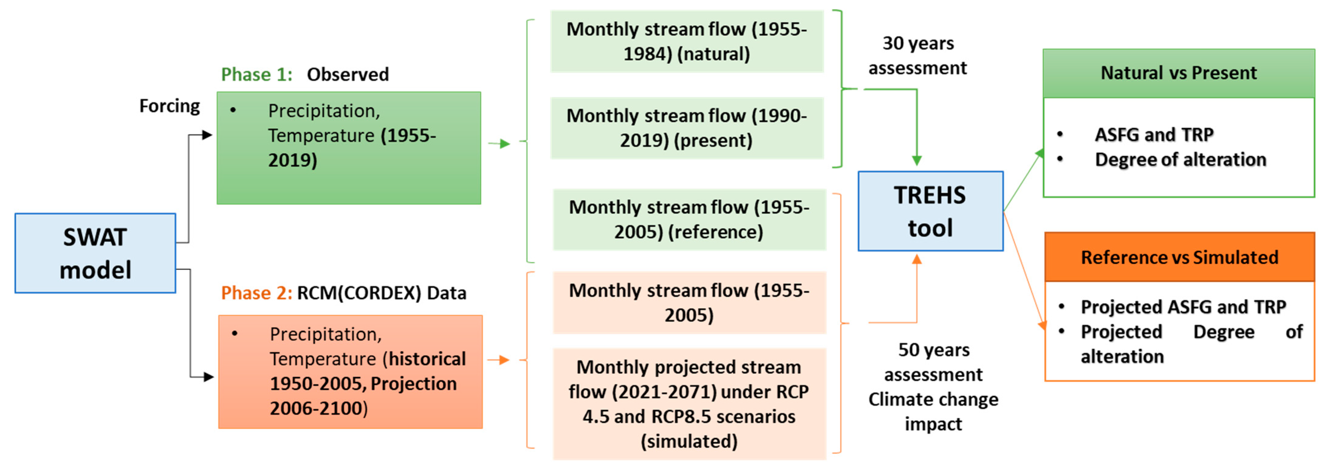
• The development and comparison of historical and future hydrological simulations by means of climatic datasets generated by multi-model ensembles of RCMs, under two different greenhouse gas emission scenarios RCP 4.5 and 8.5.
• The assessment of the potential effect of climate change, under different scenarios, on the hydrologic regime of a Mediterranean intermittent river basin and the analysis of temporal streamflow trends.
• The investigation of the transition of the different aquatic states of the stream especially from flood to edaphic, crucial for the sustainability of the ecosystem biodiversity, using the TREHS tool.

2. Study Area and Datasets

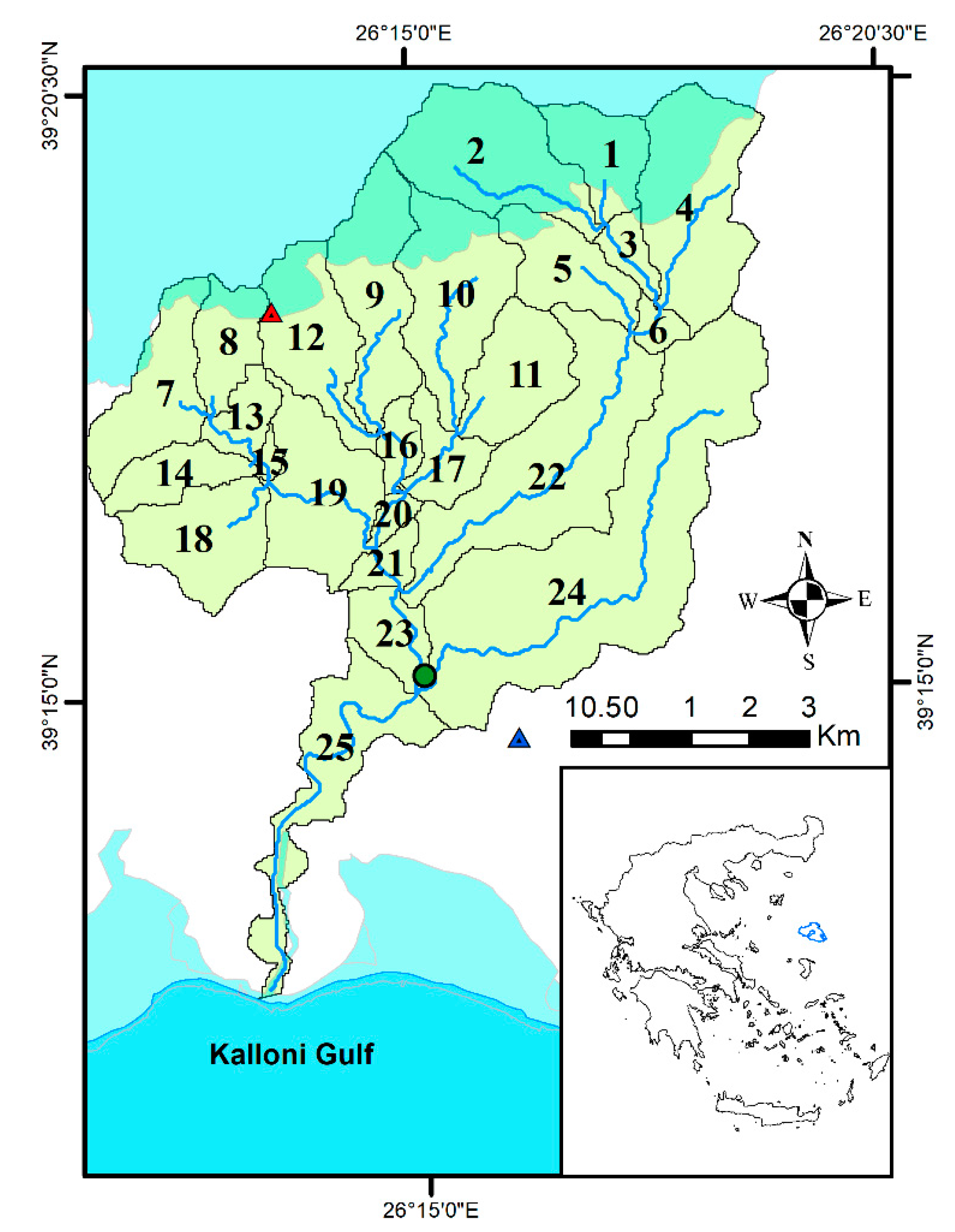
2.1. Study Area

Tsiknias is an intermittent Mediterranean stream located in the central part of Lesvos Island (Figure 1). It originates from Lepetymnos Mountain (968 m) with a mainly north to south direction and it has one of the largest drainage networks on the island [28]. The Gulf of Kalloni where this stream discharges is considered as the main ecological and touristic asset of Lesvos Island. Due to its importance regarding biodiversity and the presence of endemic species, it was established as a Natura 2000 Special Conservation Area [29].

Tsiknias basin is located between approximately 26°19′17.8026″ east and 26°10′52.1754″ west longitude, and between 39°11′50.7546″ south and 39°20′39.4902″ north latitude covering an area of approximately 90 km². The main geologic formations are of Neogene and Miocene age volcanic acidic rocks including ignimbrite, basalt, lavas, and tuffs and Pleistocene and Holocene continental deposits in the coastal part [30,31]. Most soils in this basin result from these formations. The permeability of the soils is low in most of the area, low-medium in the highland areas, and medium in the northern part of the area [32]. The major land use is agriculture (58.3%, of which olive groves cover 22.9%), followed by ryegrass (21.3%), and the remaining 20.4% is rangeland, forests, wetlands, and low-density urban areas [33].

The basin has a typical Mediterranean climate, with warm, dry summers and mild, moderately rainy winters. The mean annual temperature is 19.2 °C, and the mean annual rainfall varies from 600 mm on the plains to over 900 mm in the mountains. Since 1955, temperature has shown a slight non-uniform warming trend, while precipitation is indicating a slight decrease (Figure 2).

2.2. Spatiotemporal Datasets

Table 1. Datasets used in the present study.

Dataset	Source	Frequency	Time Period	Remarks
Rainfall	Automatic meteorological station at Agia Paraskevi	Daily	(01/01/1955–01/01/2020)	Data gaps filled with Inverse Distance Method (IDM) using data from Mytilini airport as reference station.
Temperature	Automatic meteorological station at Agia Paraskevi	Daily	(01/01/1955–01/01/2020)	Data gaps filled with Mytilini airport data corrected by the average monthly difference between this station and that of Agia Paraskevi
Stream Discharge	Telemetric Radar Level Sensor (RLS) gauging station Prini-bridge	Daily	(08/01/2014–10/31/2019)	Observed gauge data; Data gap: 11/01/2016–11/01/2017
Landuse	CORINE 2000 [34]	-	-	The map is corrected with the inclusion of five settlements and data gathered by field validation. 1:25,000
Soil	Municipality, Hellenic Survey of Geology and Mineral Exploration (HSGME), field sampling	-	-	Combined soil data from maps provided by the municipality, the HSGME and field sampling [35]
Topography	NASA Shuttle Radar Topography Mission (SRTM) Version 3.0	-	-	1° × 1° tiles at 1 arc second (about 30 m)

includes the datasets used in this study, including the Land-Use Land-Cover (LULC), Digital Elevation Model (DEM), soil datasets, meteorological forcing datasets, and observed streamflow in the selected basin. Rainfall data were obtained from rain gauge observations at both Agia Paraskevi (95 m) and Stypsi (396 m) stations. Since 2014, a telemetric station (Prini) has been operating on the main channel, providing water level data in 15 min intervals. Monthly flow measurements from the same area are used to produce the rating curve, which relates the water level to the flow.

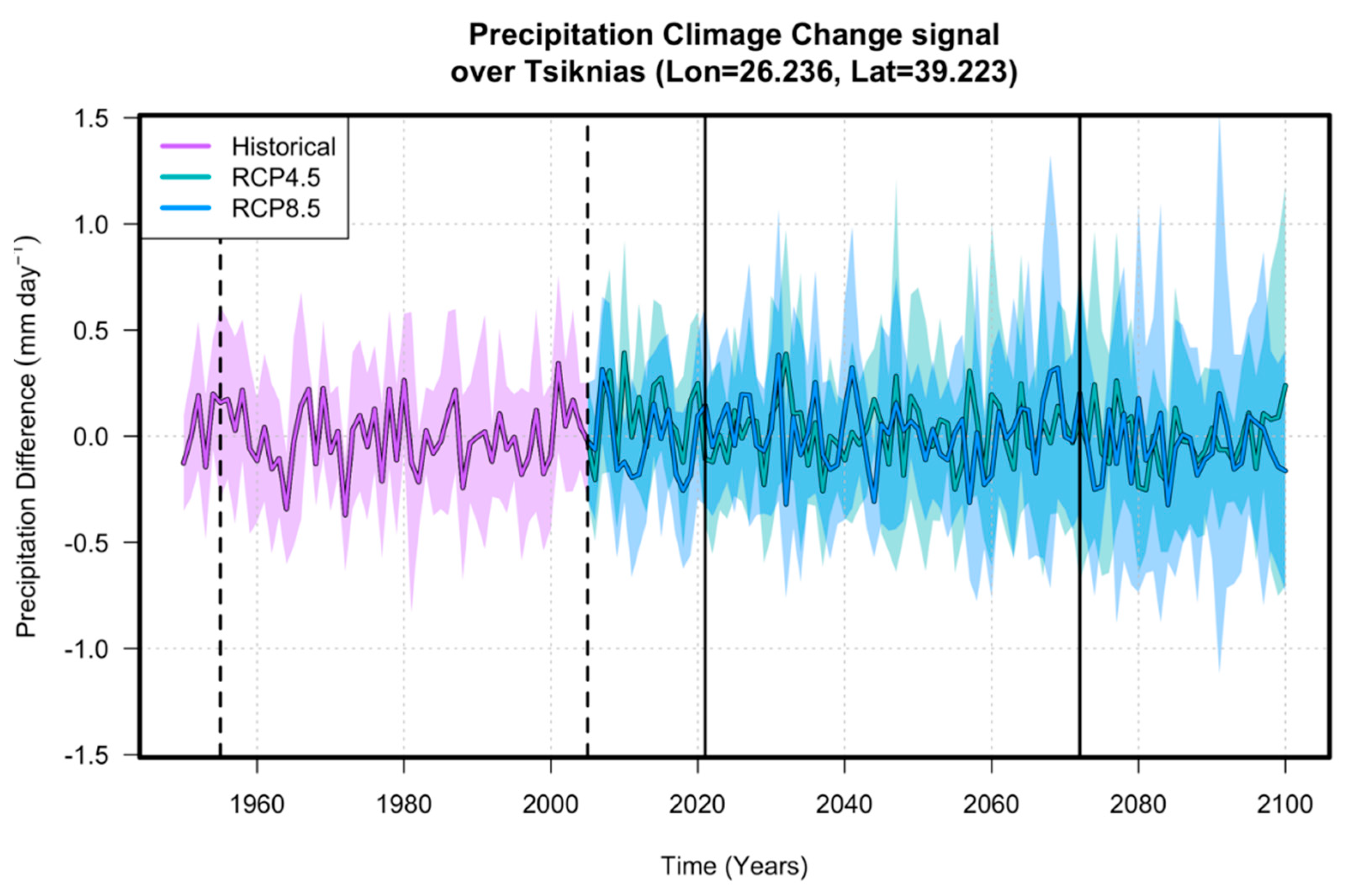
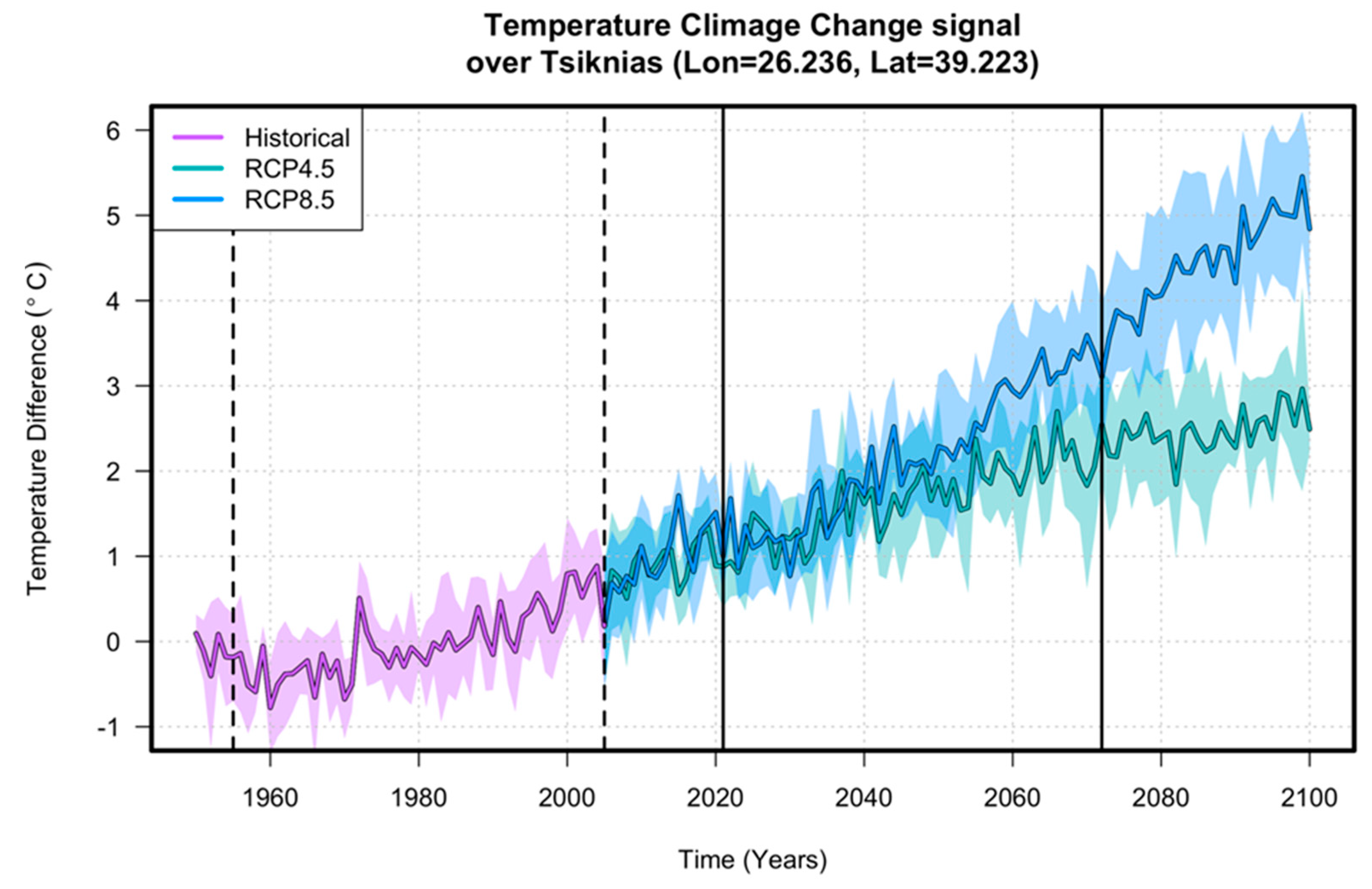
2.3. Regional Climate Model Data

The use of RCMs is necessary in regions with multiple topographic characteristics, and Greece is a Mediterranean country characterized by complex topography with steep orography from the mountainous regions to the coast, with elongated coastline and a number of small islands in the Aegean Sea and Ionian Sea. Hence, the use of dynamical downscaling to higher resolution is necessary to assess the regional and sub-regional climate of the complex topographically area of Greece [36,37].

Data series for several meteorological parameters (maximum and minimum temperature, precipitation, wind speed, and incoming shortwave radiation) of multiple RCMs, for Tsiknias basin over the time period 2021–2100, were used (

Table 2. CORDEX multi-model datasets abbreviation used in this study.

RCM Institution Name	RCM Institution Acronym	RCM Model Name	GCM Model Name	GCM Institution Acronym	Abbreviation Used in This Study
Climate Limited-area Modeling-Community	CLM com	CCLM4-8-17	CNRM-CM5	CNRM-CERFACS	CNRM-CM5_CCLM4-8-17
Centre national des recherches météorologiques	CNRM	ALADIN53	CNRM-CM5	CNRM-CERFACS	CNRM-CM5_ALADIN53
Koninklijk Nederlands Meteorologisch Instituut	KNMI	RACMO22E	EC-EARTH	ICHEC	EC-EARTH_RACMO22E
Institut Pierre-Simon-Laplace	IPSL-INERIS	WRF331F	CM5A-MR	IPSL-IPSL	CM5A-MR_WRF331F
Sveriges Meteorologiska och HydrologiskaInstitut	SMHI	RCA4	CM5A-MR	IPSL-IPSL	CM5A-MR_RCA4
Climate Limited-area Modeling–Community	CLMcom	CCLM4-8-17	HadGM2-ES	MOHC	HadGM2-ES_CCLM4-8-17
Sveriges Meteorologiska och HydrologiskaInstitut	SMHI	RCA4	HadGM2-ES	MOHC	HadGM2-ES_RCA4
Climate Limited-area Modeling–Community	CLMcom	CCLM4-8-17	MPI-ESM-LR	MPI-M	MPI-ESM-LR I_CCLM4-8-17
Max Planck Institute Magdeburg	MPI-CSC	REMO2009	MPI-ESM-LR	MPI-M	MPI-ESM-LR_REMO2009

). The projections are in a high resolution (0.11 deg) from various RCMs and emission scenarios (RCPs 4.5 and 8.5) based on data from EURO-CORDEX initiative [38]. EURO-CORDEX is the European branch of the international CORDEX initiative, which is a program sponsored by the World Climate Research Program (WRCP) to organize an internationally coordinated framework and produce improved regional climate change projections for all land regions worldwide. In this study, CORDEX results serve as input for climate change impact assessment, within the timeline of the Fifth Assessment Report (AR5). The data extraction and analysis is in the framework of GEO-CRADLE [39], which aims to provide a user-friendly web application tool for climate change impact studies, for end users and policy makers on climate change adaptation strategies.

In this work, the focus is on the changes between the future and control period, to assess future sensitivity of the hydrological regime to the climate change. Thus, no bias correction was conducted on the CORDEX RCMs meteorological datasets, since it would not have a quantitative added value; on the contrary, it may induce other uncertainties and mask the climate change effects from linear corrections in past and future, for a system that is not linear (hydrological regime). The applicability of bias correction approaches especially for extreme hydrological indicators, such as high flows, was found to have high impacts on their values and generally is still questionable [40].

3. Methodology

The methodology applied in this study is described in Figure 3 and includes the following steps: (1) setup of the SWAT model and calibration/validation using SWAT-Cup algorithm SUFI2 (see Section 3.1.2 and Section 3.1.3); (2) simulation of historical and future flow using the calibrated model forced by the CORDEX datasets (see Section 3.1.4); (3) classification of the Tsiknias River regime using metrics that measure the relative permanence of temporary flow phases within TREHS model; and (4) assessment of the degree of alteration due to climate change of the temporary regime of Tsiknias River (see Section 3.2.2).

3.1. Hydrological Modeling

3.1.1. Soil and Water Assessment Tool (SWAT)

The SWAT model was chosen because of the plethora of parameters available for a better simulation of processes specific to each basin, its flexibility during the calibration stage, and the option of running climate change scenarios. SWAT [17,18,19,41], is a continuous, semi-distributed, physically-based hydrologic model, developed by the U.S. Department of Agriculture (USDA), to predict the impact of land management practices on water, sediments, and agricultural chemical yields in large complex basins with varying soils, land use, and management conditions over long periods of time [18]. It divides a basin into sub-basins connected by a stream network and further, divides each sub-basin into Hydrologic Response Units (HRUs) consisting of unique combinations of slope, land use, and soils. Runoff is predicted separately for each HRU and routed to obtain the total runoff for the basin. This increases the accuracy and gives a much better physical description of the water balance. SWAT model operates on a daily or sub-daily time-step for each hydrologic unit based on water balance equation and simulates the hydrology into land and routing phases. During the land phase, the amount of water, sediment, and other non-point loads are calculated from each HRU and summed up to the level of sub-basins. Each sub-basin controls and guides the loads towards the sub-basin outlet. The routing phase defines the flow of water, sediments, and other non-point sources of pollution through the channel network, from one sub-basin to another and to the outlet of the basin.

The hydrological cycle simulated by SWAT is based on the water balance equation:

$$S{W}_t =S{W}_0+{\displaystyle \sum }_{i=1}^t\left(R_{day}-Q_{surf}-E_a-W_{seep}-Q_{lat}-Q_{gw}\right)$$

(1)

where SW_t is final soil water depth (mm), SW₀ is the initial soil water depth (mm), t is the time step (days), R_day is the daily precipitation (mm), Q_surf is a surface run-off (mm), E_a is the actual evapotranspiration (mm), Q_gw is the depth of water entering in vadose zone from soil profile (mm), and Q_lat is the depth of lateral flow (mm). Runoff is derived from the USDA Soil Conservation Service (SCS) runoff Curve Number (CN) method [42] as follows:

$$Q_{surf}=\frac{{\left(R_{day}-I_a\right)}^2}{\left(R_{day}-I_a+S\right)}$$

(2)

where R_day is rainfall depth for that day; I_a is the initial abstraction, which is a function of infiltration, interception and surface storage; and S is the retention parameter calculated from the curve number (CN), which is based on soil parameters and land use classes. CN is an important calibration parameter for surface runoff [19]. High CN corresponds to high overland flow often associated with developed soils, while low CN represents well-drained soils and results in low rates of surface runoff.

3.1.2. Model Setup

SWAT was setup for Tsiknias River basin through the ArcSWAT interface [43] using the land use, soil, and DEM datasets and meteorological data described in Table 1. The basin was divided into 25 sub-basins and 848 HRUs.

3.1.3. Model Calibration and Parametrization

The Tsiknias River basin was calibrated from 2014 to 2016 and validated from 2017 to 2019 on a daily time step with observed meteorological data and streamflow from Prini gauge station, with two years as a warmup period (2011–2013). The Sequential Uncertainty Fitting ver.2 (SUFI2) embedded within the SWAT Calibration and Uncertainty Program (SWAT-CUP) software [44,45,46] was employed for auto calibration, using the Nash–Sutcliffe Efficiency (NSE) as the objective function criterion. Nine parameters were selected (

Table 3. Parameters used in the calibration process.

Parameters 1	Definition	Physically Meaningful Range (min max)		Calibration Range
r__CN2.mgt	Initial SCS runoff curve number for moisture condition	35	98	−50% to 20%
v__ALPHA_BF.gw	Base flow travel time (days)	0	1	0.2−1
v__GWQMN.gw	Threshold depth of water in the shallow aquifer required for return flow to occur (mm)	0	5000	−1000–2000
r__SOL_AWC.sol	Available water capacity of the soil layer (mm/mm)	0	1	−20% to 20%
v__ESCO.hru	Soil evaporation compensation factor	0	1	0.6–1
v__REVAPMN.gw	Threshold depth of water in the shallow aquifer for revap to occur (mm)	0	500	0–500
v__GW_REVAP.gw	Ground water revap coefficient	0.02	0.2	0.02–0.2
v__LAT_TTIME.hru	Lateral flow travel time (days)	0	180	0–150
r__SLSUBBSN.hru	Average slope length (m)	10	150	−25%–25%

¹ v__ means the default parameter is replaced by a given value within calibration range; r__ means the existing parameter value is multiplied by a given value; mgt, crop cover management process; gw, groundwater process; sol, soil water dynamics process; bsn, basin scale; rte, water routing; hru, water dynamics at HRU level.

), based on dominant processes in Tsiknias basin reported by previous studies [26,47,48,49,50]. Previous streamflow measurements from July 2007 to July 2009 showed that the contribution of individual sub-basins, described in this work as Areas 1–5, respectively (Figure 4), were consistent with the size of the drainage area, the slope, and the existence of water springs [32].

The Percent Bias (PBias) [51] and NSE [52] were used to evaluate the agreement goodness of fit between observed and simulated data. In general, model simulation is regarded satisfactory if NSE > 0.50 and PBIAS = ±25% when simulated and observed streamflow are compared [53,54]. The parameter set that produced the best-fit stream discharge for the daily data was selected.

3.1.4. Future Streamflow Projections

After confirming SWAT model capability for hydrologic modeling during the previously selected time period (Section 3.1.3), CORDEX data (minimum and maximum air temperature, precipitation, wind speed, incoming shortwave radiation, and relative humidity) were applied to the calibrated SWAT model for the control period 1950–2005 to simulate historical monthly flow. Finally, CORDEX RCMs projected climate data under RCP 4.5 (intermediate scenario) and RCP 8.5 (worst-case scenario) [5] were used for simulating future monthly streamflow projections. The future time period of the simulation is 50 years (i.e., 2021–2071), having the same length as the control time period (i.e., 1955–2005).

3.2. Aquatic States (AS), Flow Regime (FR) Status, and Alteration Flow Regime (AFR) Assessment

In this section, the aquatic states are defined, TREHS tool is described (Section 3.2.1), and the methodology followed to identify the different distribution of AS, FR, and AFR for Tsiknias River due to climate change effect is analyzed (Section 3.2.2).

3.2.1. Temporary Rivers Ecological and Hydrological Status (TREHS)

TREHS was developed as a tool for applying the methods formulated during the MIRAGE Project [14], aiming to help managers capture the temporary stream dynamic and discover the convenient methods to define hydrological and ecological status [16,55,56]. By means of updated methods and visualization options, the tool facilitates the assessment of the hydrology of temporary rivers. Diverse types of hydrological-related data sources can be used to define the specific regime of temporary rivers, the aquatic states and the degree of their alteration [16,57]. for instance, monthly flow data obtained from monitoring stations, or in the case of absence of observed data, which is the case in most of intermittent rivers, rainfall–runoff model simulations, terrestrial photography, and/or interviews of locals.

TREHS defines six different AS, which correspond to the transient sets of aquatic mesohabitats occurring on a given river reach at a particular moment, depending on the hydrological conditions [14,16,56,58], allowing a better evaluation of biological assemblages [14]. From wet to dry ASs are classified as follows: flooding conditions (Hyperrheic); full prevalence of all the possible mesohabitats (Eurheic); sequence of pools connected by flowing water threads (Oligorheic); occurrence of isolated pools (Arheic); disappearance of surface water, with the wet alluvium still allowing underground aquatic life (Hyporheic); and the desiccation of the riverbed and alluvium, involving the disappearance of any active aquatic habitat (Edaphic).

The identification of the temporal patterns of occurrence of these ASs is determined based on the statistics of the occurrence of these diverse aquatic states [57,58]. The flowing water phase (Hyperrheic, Eurheic, and Oligorheic) is separated from the zero flow phase (Arheic, Hyporheic, and Edaphic) using flow threshold values, which can be identified by field observations of the ASs for more accuracy or automatically in TREHS tool by the shape of flow duration curve.

This flow duration analysis, which also characterizes the ability of the basin to provide flows of various magnitudes [59] in a given period, is identified by ranking the flow data from highest to lowest and assigning an exceedance probability, P, to each value according to the following formula:

$$\mathrm{P}=\frac{\mathrm{m}}{\mathrm{n}+1}$$

(3)

where P is the probability of exceedance, m is the rank of the data value (m = 1 being the largest), and n is the total number of data points.

The six metrics reflecting patterns of flow, isolated pools, and dry beds, for each data source are defined as follows: flow permanence (Mf), dry channel permanence (Md), isolated pool permanence (Mp), seasonal six-month predictability of the period without flow (Sd6), equinox-solstice seasonality (ESs), and summer-winter seasonality (SWs) [56,58]. The most important metrics are Mf and Sd6. They are used for the classification of flow into positive and zero flows, which have the most impact on the ecosystems of the stream [16,56,58]. Mf represents the long-term mean annual relative number of months with flow, which ranges between 0 (always dry) and 1 (always flowing). Sd6 signifies the seasonality of the dry conditions and hence the predictability of habitat availability, and it is described by the following equation [16].

$$\mathrm{Sd}6=1-{\displaystyle \sum }_1^6{\mathrm{Fd}}_{\mathrm{i}}/{\displaystyle \sum }_1^6{\mathrm{Fd}}_{\mathrm{j}}$$

(4)

where Fdi is the multi-annual frequency of zero-flow month i for the contiguous six wetter months of the year and Fdj is the multi-annual frequency of zero-flow month j for the remaining six drier months.

3.2.2. ASs, FR, and AFR Assessment Workflow

In summary the methodology followed to evaluate and determine the AS and the temporary FR in both natural and impacted (climate change) conditions of the Tsiknias temporary regime, is described Figure 4.

In the first part (Figure 4), natural AS (1955–1984) and present AS (1990–2019) were evaluated, using simulated monthly flow at one station scale, forced by observed meteorological datasets, and then were compared to each other to determine the degree of alteration. These were visualized by three plots provided by TREHS tool: (a) the Aquatic States Frequency Graph (ASFG) that shows the relative importance of the diverse states throughout the year and the degree of seasonality of the regime; (b) the Temporary Regime Plot (TRP) which presents the flow permanence against seasonal predictability in order to compare the occurrence of flow for different rivers (Permanent (P), Intermittent–Permanent (I-P), Intermittent–Dry (I-D), and Ephemeral (E)); and (c) the Flow-Pools-Dry plot (FPD) using the flow, pool, and dry permanence indicators [16].

Finally, using the projected monthly stream flows under RCP 4.5 and RCP 8.5 scenarios, we estimated the projected impacted aquatic states and their alteration. Similarly, to Part 1, results are presented in ASFG, TRP, and FDP plots.

4. Results

4.1. Hydrologic Modeling

In this section, the calibration and validation results of the SWAT hydrological model are discussed.

Table 4. Parameters used in calibration process.

Parameter	Best Simulation Fitted Value	p Value	Final Range (min, max)
r__CN2.mgt	−0.08	0.00	−0.15, −0.008
r__SLSUBBSN.hru	−0.435	0.01	−0.8, −0.08
v__GWQMN.gw	0.26	0.04	−0.17, 0.7
v__ESCO.bsn	0.783	0.05	0.72, 0.83
v__ALPHA_BF.gw	0.67	0.32	0.5, 0.8
r__SOL_AWC.sol	−0.005	0.39	−0.05, 0.05
v__LAT_TTIME.hru	16.65	0.46	0, 57.6
v__REVAPMN.gw	113.75	0.5	16.9, 210.6
v__GW_REVAP.gw	0.122	0.72	0.1, 0.15

shows the obtained calibrated fitted value for each parameter for Tsiknias basin, while Figure 5 and Figure 6 illustrate the resulting hydrographs of calibration and validation process at a daily time step.

All calibrated parameters are within the expected range for Tsiknias basin, with the most sensitive parameters being CN2, SLSUBBSN, and ESCO considering their p values. The model sensitivity to SLSBBSN confirms a previous study indicating that the size of the drainage area and the slope have great impact on the outflow within this basin (the highest elevation is 943 m and the lowest is −1 m) [32]. The small final fitted range of CN2 indicates low run-off potential of the basin due to land-use coverage, mostly agricultural (olive groves), significant natural cover such as coniferous forests in the northern part of the basin, grassland, and brushland habitats [48].

Statistical evaluations of both calibration and validation, as shown in Figure 5 and Figure 6, are within the acceptable levels reported in the literature (NSE values > 0.5, Pbias < 25%) [54]. The results show a positive correlation between the observed and simulated river flows and the water mass balance of Tsiknias River at annual scale. The simulated flow was slightly underestimated during the autumn; it sharply increases during the winter and levels off after the end of the wet period. SWAT, however, does not entirely capture both peaks in February 2015; it slightly overestimates it (Figure 5 and Figure 6). The validation flow records represent a time period during which the gauging and meteorological station are not adequately preserved, and sediment and debris have altered the examined river cross section.

Since the TREHS model requires monthly data to assess the temporary regime aquatic state and alteration, keeping the same calibrated parameters, SWAT model was run on a monthly timestep. Figure 7 shows the resulting hydrograph during the 2014–2019 period. The contribution of the different tributaries of the basin [32] was evaluated, compared to the total basin discharge, and confirmed. The main tributary referred to as Area 1 (Figure 2) is the main water contributor during the wet period (Figure 7, Subbasin 22 outflow) due to the high elevation difference, its great drainage area (30% of the basin), and the existence of spring sources. The secondary tributary (Area 4, Subbasin 20 outflow, 20% of total surface of basin) and the ephemeral tributaries (Areas 3 (Subbasin 24) and 2 (Subbasin 19), covering 15% and 17%, respectively) equally contribute less water to the main stream (Area 5, Subbasins 23 and 25 outflow). The ephemeral tributaries are showing a steeper reduction during spring in the end of the wet season, attributed to their ephemeral nature. The discharge at the Prini station of Tsiknias River corresponds to the sum of the outflows from the contributing streams. Correspondingly, the low slope at the lowland area near the outlet allows for higher infiltration with regards to the upstream parts of the basin and experiences higher groundwater recharge rates, resulting in zero flow during the dry period.

4.2. Future Climate

Based on high resolution regional climate data (0.11°) acquired from CORDEX, the multi-model simulated time series of changes in the annual precipitation and temperature relative to the period 1961–1990 for the scenarios RCP 4.5 and RCP 8.5 as well as the historical period are shown in Figure 8 and Figure 9. The lines indicate ensemble yearly means from the yearly ensemble mean data. All precipitation scenarios for the future indicate a slight but not robust decrease of precipitation, while temperature projections show warming trends for the different RCPs (highest for RCP 8.5 and lowest for RCP 4.5) which drift apart significantly during the second half of the 21 century. During the same period, the ensemble standard deviation (shaded area) is increasing, indicating a rise in the uncertainty of the simulated ensemble temperature and precipitation.

The projected climate variable of rainfall for the future period (2021–2071) under both RCPs was analyzed against the baseline situation (1955–2005). The precipitation mean monthly cycles are presented in Figure 10 for the historical period, RCP 4.5, RCP 8.5, and observed. Both RCP 4.5 and RCP 8.5 scenarios project a decrease in precipitation mostly during the wet season.

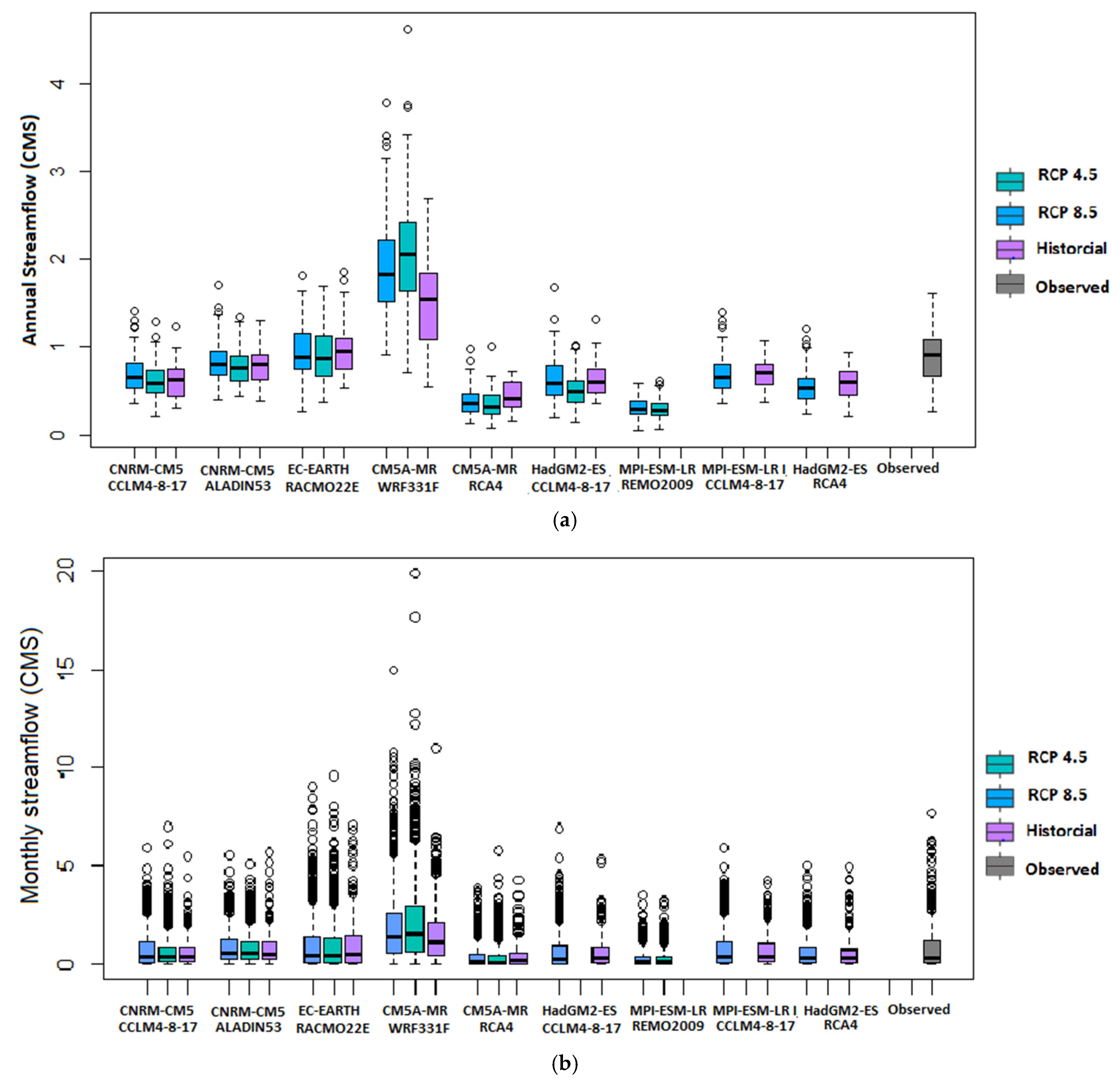
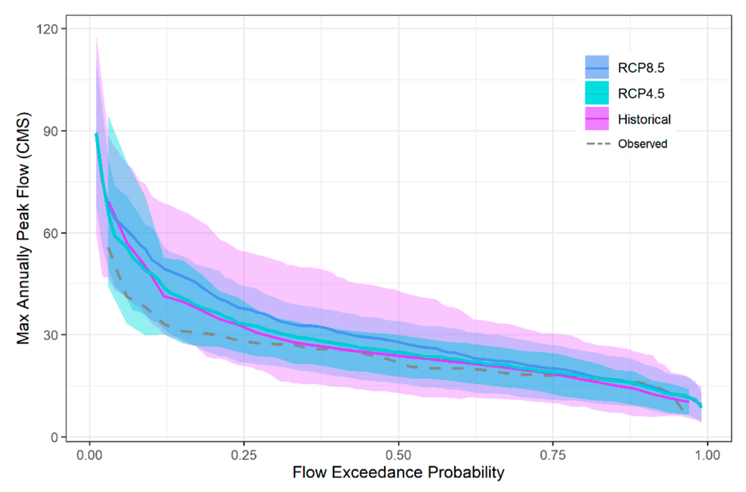
4.3. Future Streamflow Projections (Monthly and Annual)

Figure 11 presents boxplots of the streamflow distributions of the control period (1955–2005) and future streamflow projections (from 2021 to 2071 under RCP 4.5 and 8.5 scenarios) forced by CORDEX RCMs datasets listed in Table 2 compared with the reference period (1955–2005) simulated by SWAT model. How well different RCMs capture characteristics of the reference flow distribution and the change future scenarios is indicated. Primary evaluation of the simulated outflow for the historical climate (1955–2005) against simulated streamflow shows that the annual and monthly observations are captured well by the ICHEC_KNMI model, unlike other RCMs. Analysis of the future scenarios (2021–2071) projections of the RCM/GCM ensembles for all models shows an increase in extreme events occurrence. Ultimately, almost all RCMs show a decrease in flow in the future and higher occurrence of extreme flood events highlighted by the presence of outliers (Figure 11).

In Figure 12, the actual flow duration curve of Tsiknias streamflow is compared to flows generated from RCM simulated flow. Most models generally replicate the flow pattern, yet exhibit major differences, particularly in low flows. As for the future, a higher frequency of low flows is projected, as well as an increase of the frequency of mid-range and high flows (Figure 12).

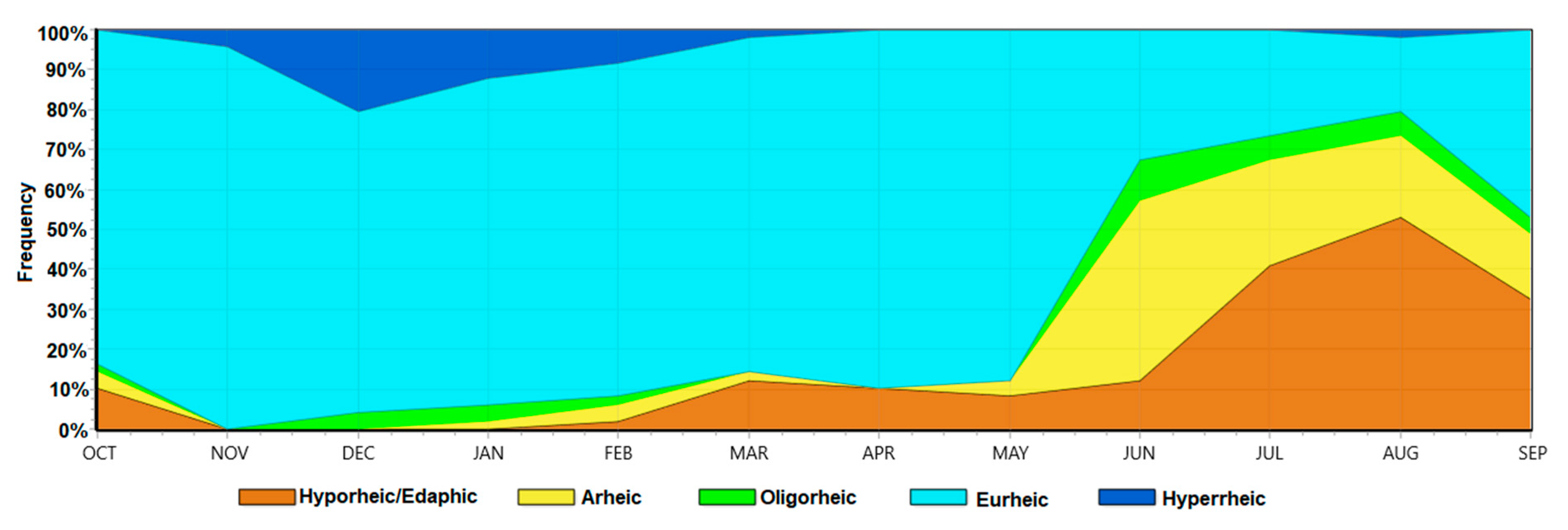
4.4. Hydrological Status

Tsiknias River is characterized by a temporary hydrological regime subject to seasonal abstraction in order to cover irrigation needs; it is, therefore, prone to more alteration [26]. Assessment of the current and projected future flow regimes, however, is important to understand the existing ecosystems functioning and river processes sustainability. In this section, the classification of Tsiknias flow regime and the distribution of the aquatic states is evaluated firstly, under natural (1955–1984) and present (1990–2019) conditions. Then, using CORDEX RMCs simulated monthly flows, the projected conditions (2021–2071) are gauged.

4.4.1. ASFG (Natural, Actual, and Projected)

The ASFG describes the relative frequency (%) of the aquatic states through the year, which is derived from the monthly frequencies of the simulated flows. It is generally applied for the selection of the most appropriate sampling methods (e.g., biomonitoring) according to the temporal variability and seasonal predictability of the transient sets of aquatic mesohabitats occurring in a stream [56], but also for the visualization of the flow regime of the streams. The threshold values between flow phases were fixed automatically in TREHS based on the flow duration curve. The ASFG was first generated for Tsiknias River during the natural state (1955–1984) and actual state (1990–2019) (Figures S1–S3), natural state represents the period with the minimum human intervention to the flow regime and the absence of any irrigation projects.

Figure 13 shows ASFG obtained from reference discharge (1955–2005) simulated by the calibrated SWAT model. Under natural state, Tsiknias River exhibits clear seasonality (dry summer and relatively wet winter). The permanence of the flow is considerable (Eurheic 83.7%, indicating full prevalence of all the possible mesohabitats), although it dries more than 10% of the time.

After describing the actual flow regime of Tsiknias River, its assessment under different scenarios, RCP 4.5 and RCP 8.5, can be useful for decision makers for taking appropriate measures to mitigate the alteration of flow regimes due to the impact of climate change. The same methodology was used during the assessment of the aquatic state frequency. Figure 14 shows a set of ASFGs obtained from diverse RCM simulations under both scenarios (RCP 4.5 and RCP 8.5) to determine the possible scenarios of alteration of the aquatic states due to climate change. According to the ASGF graphs (Figure 14), most RCMs indicate that Tsiknias River will be affected by increasing dry state and low flows periods under both RCP 4.5 and RCP 8.5 scenarios. CM5A-MR_RCA4 and MPI-ESM-LR_REMO2009 models on the other hand show a different pattern and loss of seasonality. HadGM2-ES_CCLM4-8-17 and HadGM2-ES_RCA4 models show a different pattern even in the historical period.

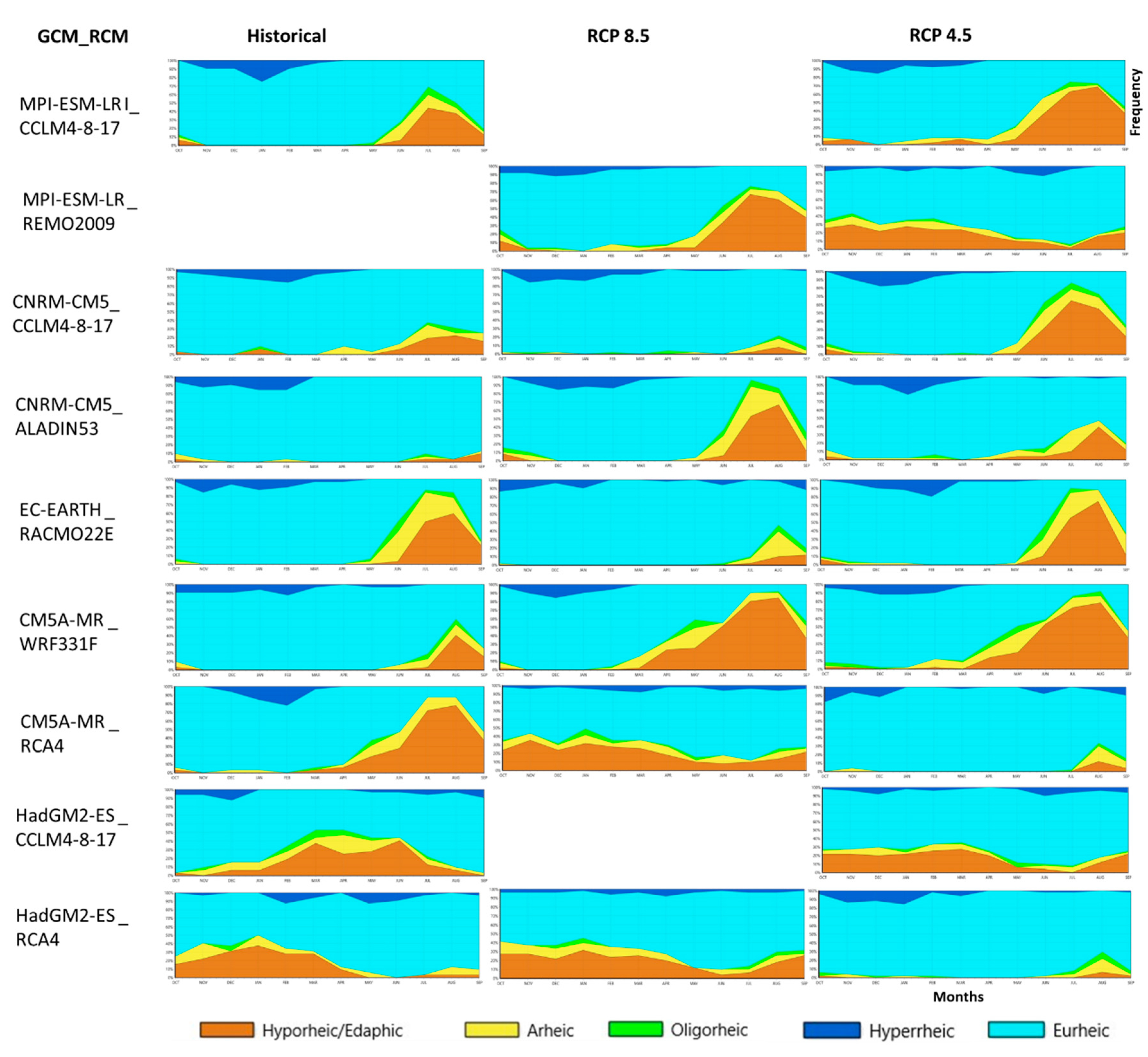
4.4.2. Projected Temporary Regime Alteration

The metrics of flow permanence, Mf, and seasonal predictability of dry periods, Sd6, were first evaluated for Tsiknias River in unimpacted (natural) and impacted conditions (climate change) using the SWAT simulated monthly outflows. The results are shown in TRP graphs (see the Supplementary Materials). They provide a classification of the river types, where the intermittence of the river increases from the upper right corner to the lower left. Gallart et al. (2012) [56] defined the limits between regime types in the Mediterranean region by analyzing flow time series from different streams within this area, which are Permanent (P), Intermittent–Permanent (I-P), Intermittent–Dry (I-D), and Ephemeral (E). They are differentiated by the grey lines on the graph. Furthermore, climate change impact on Tsiknias temporary regime was assessed by analyzing the shift between corresponding points of RCMs under both scenarios and natural conditions point. Analysis indicates the projected possible alteration degree of Tsiknias flow regime, due to the changes occurring in flow permanence (Mf) and dry season predictability (Sd6) (Figure 15). The results in the TRP indicate that the actual state of Tsiknias stream is Intermittent–Permanent (I-P) and the stream keeps this aquatic state according to many climate change scenarios. Both RCP 4.5 and RCP 8.5 scenarios predict a shift in the aquatic state to I-P. The distance between the corresponding points in unimpacted and impacted conditions is an indicator of the hydrological regime alterations capturing a shift in flow permanence. The FPD graphs are divided into nine aquatic phase regime classes based on three metrics corresponding to the proposed three aquatic phases: flow permanence, isolated pools permanence, and dry river permanence [16]. According to the reference period, Tsiknias River exhibits an alternate fluent regime (0.40 < Mf ≤ 0.90, 0.00 ≤ Mp < 0.50, and 0.10 ≤ Md < 0.60), meaning that it rotates between three aquatic phases. In impacted conditions, however, most models under both RCPs scenarios generally indicate an alternate–fluent regime with a decrease in dry and pool permanence (Figure 16). CM5A-MR_WRF3331F and CNRM-CM5_ALADIN53 models exhibit a shift from a quasi-perennial regime in reference conditions to an alternate–fluent aquatic regime. HadGM2-ES_CCLM4-8-17 and HadGM2-ES_RCA4 models indicate a shift in the opposite direction under RCP 4.5 and RCP 8.5.

5. Discussion

CORDEX RCM data were used to assess the climate change impact on the Tsiknias River hydrological regime. The results indicate that Tsiknias basin will suffer a combination of increased temperature and slightly reduced rainfall that will directly impact the flow regime; similar findings have been found in different parts of Mediterranean region [20,60,61,62]. The results of some RCMs simulations, however, do not capture the observed flow seasonality, which calls for further analysis, as it will provide further insight into projected climate model data and improve the accuracy of results, therefore improving the climate change impact adaptation strategies [60].

Analysis of the difference between the flow regime and distribution of its different aquatic states, based on the monthly average river discharge, the permanence of flow, and the six-month dry season predictability, between natural and present conditions, displays little to no alteration; nevertheless, in a neighboring watershed in Italy [62], the alteration was observed mostly downstream of the studied basin. Projected temperature increase and precipitation decrease, however, are expected to induce a change in the future flow regime, which exhibits an increase in summer and decrease in winter of flood events. These results are echoed in other studies within the Mediterranean region [63,64]; the predictions indicate high flow magnitudes will increase, the dry season will be extended, and extreme low flow conditions will be more aggravated. Furthermore, the major threat on the ecohydrological regime is expected in the last 30 years of the twenty-first century [63].

Using hydrological modeling for the reconstruction of the streamflow within an ungauged river basin and over the historical period is useful when observed data are missing [10]. In that scope. SWAT model was able to simulate streamflow in temporary river system, and therefore used to generate future flows to assess the projected hydrological regime of Tsiknias River. The variability of the aquatic states and thus ecosystems of temporary rivers make them more prone to be severely threatened by hydrological alteration [12]. Tsiknias River was identified as a temporary stream, which is the case of more than 50% of Mediterranean rivers [65]. Furthermore, it was concluded that high and low flows will become more extreme and dry periods will extend for longer periods as a result of climate change impact under both scenarios RCP 4.5 and RCP 8.5. These results resonate with different studies conducted in Europe [66] and the Mediterranean region in particular [6,12,67,68,69].

TREHS tool was tested and subsequently applied to assess the hydrological regime of temporary regime, however the ecological response to hydrological alterations was not evaluated, due to lack of data. Additionally, this model was previously tested on 119 stations from the Catalan River basin district, the Júcar River basin district, and the Ebro River basin district in Spain by the developers [16]. The results of these studies can be found in the TREHS database, allowing a comparison with other stations within the Mediterranean region. However, due to some limitations in the visualization of the results, this feature was not explored. Furthermore, using other methods offered by the TREHS tool such as photometry, observations, and interviews, is still to be explored. This tool is very useful and can be more advantageous due to rapid technological advancements in sensors and the massive penetration of smartphone technologies, which could facilitate the engagement of citizens in data collection in the context of hydrology, thus enhancing the long-term sustainability of monitoring networks [70].

6. Conclusions

In the present study, the assessment of flow and possible alteration of the hydrological and ecological status due to climate change impacts on the intermittent stream of Tsiknias stream was addressed, using hydrological modeling and ecological assessment. SWAT model with its plethora of available calibration parameters proved flexible enough during calibration and was able to reproduce the outflow of Tsiknias stream satisfactorily. Next, the calibrated model was run for historical (1955–2005) and projected (2021–2071) periods under RCP 4.5 and RCP 8.5 using CORDEX model simulations. The predicted increase in temperature and decrease in precipitation in the future resulted in a decrease of flow in the future and higher occurrence of extreme flood events captured with almost all RCM model simulations.

Using the flow records and RCMs simulated by SWAT flows, the present and projected four ASs of Tsiknias River were determined using the TREHS model. The ASFG of the actual flow is made exclusively with the use of the existing streamflow records without exploring the available options of aerial photography and interviews, which could have had a positive impact on the obtained results. The ASFGs showed high variability of the aquatic states in the future with a clear loss of the flow seasonality and an increase of the dry (Arheic and Hyporheic) states. The majority of the climate change scenarios predict an increase of the extreme flood events and expansion of the dry aquatic states of the IRES. The occurrence of extreme events is distributed not only to the winter months but in some cases to the whole year period. The ecosystem of this intermittent flow river is vulnerable to all these changes, with higher fragility in the flow-pool conditions, depicting future droughts, harming the local agriculture, ecological systems, and the socioeconomic life. Therefore, water retention measures could be considered such as the construction of reservoirs to store water and the adaptation of a set of nature-based solutions (i.e., small dams, weirs, and riparian restoration) to shield from future extreme flood phenomena.

IRES are complex hydrological systems. However, there are important obstacles for their proper study such as the hydrological or spatial information. The use of distributed models such as SWAT can facilitate the understanding of their response to the various human interventions and to the climate change impact. Finally, the application of the TREHS tool constitutes a great asset in defining the environmental flow requirements to prevent the degradation of these ecological pillars.

References

1. The European Communites Directive 2000/60/EC of the European Parliament and of the Council of 23 October 2000 Establishing a Framework for Community Action in the Field of Water Policy; Official Journal of the European Communities: Brussel, Belgium, 2000; Volume OJ L 327, pp. 1–73.
2. Datry, T.; Singer, G.; Sauquet, E.; Jorda-Capdevila, D.; Von Schiller, D.; Stubbington, R.; Magand, C.; Pařil, P.; Miliša, M.; Acuña, V.; et al. Science and Management of Intermittent Rivers and Ephemeral Streams (SMIRES). Res. Ideas Outcomes 2017, 3, e21774. [Google Scholar] [CrossRef]
3. Kaletová, T.; Loures, L.; Castanho, R.A.; Aydin, E.; da Gama, J.T.; Loures, A.; Truchy, A. Relevance of intermittent rivers and streams in agricultural landscape and their impact on provided ecosystem services—A mediterranean case study. Int. J. Environ. Res. Public Health 2019, 16, 2693. [Google Scholar] [CrossRef] [PubMed] [Green Version]
4. Datry, T.; Larned, S.T.; Tockner, K. Intermittent rivers: A challenge for freshwater ecology. Bioscience 2014, 64, 229–235. [Google Scholar] [CrossRef] [Green Version]
5. IPCC. Climate Change 2013; IPCC: Geneva, Switzerland, 2014; Volume 5, ISBN 9781107661820. [Google Scholar]
6. Loizidou, M.; Giannakopoulos, C.; Bindi, M.; Moustakas, K. Climate change impacts and adaptation options in the Mediterranean basin. Reg. Environ. Chang. 2016, 16, 1859–1861. [Google Scholar] [CrossRef] [Green Version]
7. Pachauri, R.K. Climate Change 2014 Synthesis Report; IPCC: Geneva, Switzerland, 2014; ISBN 9789291691432. [Google Scholar]
8. Giorgi, F.; Lionello, P.; Ictp, A.S.; Lecce, U. Climate Change Projections for the Mediterranean Region Submitted to Global and Planetary Change Special Issue on Mediterranean climate variability Abstract Key words: Climate change, Mediterranean climate, Precipitaton change, Temperature change. Glob. Planet. Chang. 2008, 63, 90–104. [Google Scholar] [CrossRef]
9. Alpert, P.; Krichak, S.O.; Sha, H.; Haim, D.; Osetinsky, I. Climatic trends to extremes employing regional modeling and statistical interpretation over the E. Mediterranean. Glob. Planet. Chang. 2008, 63, 163–170. [Google Scholar] [CrossRef]
10. Fonseca, A.R.; Santos, J.A. Predicting hydrologic flows under climate change: The Tâmega Basin as an analog for the Mediterranean region. Sci. Total Environ. 2019, 668, 1013–1024. [Google Scholar] [CrossRef]
11. Zittis, G.; Hadjinicolaou, P.; Klangidou, M.; Proestos, Y.; Lelieveld, J. A multi-model, multi-scenario, and multi-domain analysis of regional climate projections for the Mediterranean. Reg. Environ. Chang. 2019, 19, 2621–2635. [Google Scholar] [CrossRef] [Green Version]
12. Tzoraki, O.; Girolamo, A.D.; Gamvroudis, C.; Skoulikidis, N. Assessing the flow alteration of temporary streams under current conditions and changing climate by Soil and Water Assessment Tool model. Int. J. River Basin Manag. 2015, 1–10. [Google Scholar] [CrossRef]
13. Cramer, W.; Guiot, J.; Fader, M.; Garrabou, J.; Gattuso, J.P.; Iglesias, A.; Lange, M.A.; Lionello, P.; Llasat, M.C.; Paz, S.; et al. Climate change and interconnected risks to sustainable development in the Mediterranean. Nat. Clim. Chang. 2018, 8, 972–980. [Google Scholar] [CrossRef] [Green Version]
14. Prat, N.; Gallart, F.; Von Schiller, D.; Polesello, S.; García-Roger, E.M.; Latron, J.; Rieradevall, M.; Llorens, P.; Barberá, G.G.; Brito, D.; et al. The Mirage Toolbox: An Integrated Assessmen TOOl for Temporary Streams. River Res. Appl. 2014, 30, 1318–1334. [Google Scholar] [CrossRef]
15. Gauthier, M.; Launay, B.; Le Goff, G.; Pella, H.; Douady, C.J.; Datry, T. Fragmentation promotes the role of dispersal in determining 10 intermittent headwater stream metacommunities. Freshw. Biol. 2020, 65, 2169–2185. [Google Scholar] [CrossRef]
16. Gallart, F.; Cid, N.; Latron, J.; Llorens, P.; Bonada, N.; Jeuffroy, J.; Jiménez-Argudo, S.-M.; Vega, R.-M.; Solà, C.; Soria, M.; et al. TREHS: An open-access software tool for investigating and evaluating temporary river regimes as a first step for their ecological status assessment. Sci. Total Environ. 2017, 607–608, 519–540. [Google Scholar] [CrossRef] [PubMed]
17. Santhi, C.; Srinivasan, R.; Arnorld, J.; Williams, J. A modeling approach to evaluate the impacts of water quality management plans implemented in a watershed in Texas. Environ. Model. Softw. 2006, 21, 1141e1157. [Google Scholar] [CrossRef]
18. Neitsch, S.; Arnold, J.G.; Kiniry, J.; Williams, J. Soil and Water Assessment Tool Theoretical Documentation Version 2009; Texas Water Resources Institute: College Station, TX, USA, 2009. [Google Scholar]
19. Arnold, J.G.; Moriasi, D.N.; Gassman, P.W.; Abbaspour, K.C.; White, M.J.; Srinivasan, R.; Santhi, C.; Harmel, R.D.; van Griensven, A.; Liew, M.W.; et al. SWAT: Model Use, Calibration, and Validation. Trans. ASABE 2012, 55, 1317–1335. [Google Scholar] [CrossRef]
20. Abouabdillah, A.; Oueslati, O.; Girolamo, A.M.D.; Porto, A.L. Modeling the impact of climate change in a mediterranean catchement (merguellil, Tunisia). Fresenius Environ. Bull. 2010, 19, 2334–2347. [Google Scholar] [CrossRef]
21. Papatheodouliu, A.; Tzoraki, O.; Panagos, S.; Taylor, H.; Ebdon, J.; Papageorgiou, G.; Pissarides, N.; Antoniou, K.; Christofi, G.; Dorlfinger, G.; et al. Simulation of daily discharge using the distributed model SWAT as a catchment management tool: Limnatis River case study. Proc. SPIE Int. Soc. Opt. Eng. 2013. [Google Scholar] [CrossRef]
22. Tzoraki, O.; Cooper, D.; Kjeldsen, T.; Nikolaidis, N.P.; Froebrich, J.; Querner, E.; Gallart, F. Flood generation and classification of a semi-arid intermittent flow watershed: Evrotas river. Int. J. River Basin Manag. 2013, 11, 77–92. [Google Scholar] [CrossRef]
23. De Girolamo, A.; Gallart, F.; Pappagallo, G.; Santese, G.; Lo Porto, A. An eco-hydrological assessment method for temporary rivers. The Celone and Salsola rivers case study (SE, Italy). Ann. Limnol. Int. J. Limnol. 2015, 51, 1–10. [Google Scholar] [CrossRef] [Green Version]
24. D’Ambrosio, E.; De Girolamo, A.M.; Barca, E.; Ielpo, P.; Rulli, M.C. Characterising the hydrological regime of an ungauged temporary river system: A case study. Environ. Sci. Pollut. Res. 2017, 24, 13950–13966. [Google Scholar] [CrossRef]
25. Oueslati, O.; Girolamo, A.M.D.; Abouabdillah, A.; Kjeldsen, T.R.; Porto, A.L. Classifying the flow regimes of Mediterranean streams using multivariate analysis. Hydrol. Process. 2015, 4682, 4666–4682. [Google Scholar] [CrossRef]
26. Tzoraki, O. Operating Small Hydropower Plants in Greece under Intermittent Flow Uncertainty: The Case of Tsiknias River (Lesvos). Challenges 2020, 11, 17. [Google Scholar] [CrossRef]
27. Angela, D.; Krystalia, E.; Vaia, D.; Epaminondas, L.; Costas, A.; Panayiota, K.; Nikos, P.; Arsinoe, S.; Skevi, S.; Yioannis, B.; et al. Temporal and inter habitat variations of substratum, vegetation and substratum macroinvertebrates attributes across coastal wetland systems, North East Aegean, Greece. Transit. Waters Bull. 2008, 2, 1–16. [Google Scholar] [CrossRef]
28. Spyropoulou, A.; Spatharis, S.; Papantoniou, G.; Tsirtsis, G. Potential response to climate change of a semi-arid coastal ecosystem in eastern Mediterranean. Hydrobiologia 2013, 705, 87–99. [Google Scholar] [CrossRef]
29. Natura 2000 European Environment Agency (EEA), The Natura 2000 Protected Areas Network; EEA: Copenhagen, Denmark, 2000.
30. Borsi, S.; Ferrara, G.; Innocenti, F.; Mazzuoli, R. Geochronology and Petrology of Recent Volcanics in the Eastern Aegean Sea (West Anatolia and Lesvos Island). Bullin Volcanol. 1972, 81, 473–496. [Google Scholar] [CrossRef]
31. Pe-Piper, D.J.W. Spatial and temporal variation in Late Cenozoic volcanic rocks, Aegean Sea region. Tecronophysics 1989, 169, 113–134. [Google Scholar] [CrossRef]
32. Polatidou, M.; Tsirtsis, G.; Gaganis, P. Assessing nutrient dynamics in a small eastern mediterranean watershed. In Proceedings of the 13th International Conference on Environmental Science and Technology—CEST2013, Athens, Greece, 5–7 September 2013; pp. 5–7. [Google Scholar]
33. CLC 2000—Copernicus Land Monitoring Service. Available online: https://land.copernicus.eu/pan-european/corine-land-cover/clc-2000?tab=metadata (accessed on 16 February 2021).
34. Haines Young, R.; Weber, J.L. Land Accounts for Europe 1990–2000: Towards Integrated Land and Ecosystem Accounting; EEA: Copenhagen, Denmark, 2006; Volume 11. [Google Scholar]
35. Provatas, N. Time and Spatial Analysis of Water Quality in Insular Basins: The Case of Tsiknias River, Lesvos; University of the Aegean: Mytilene, Greece, 2015. [Google Scholar]
36. Zanis, P.; Kapsomenakis, I.; Philandras, C.; Douvis, K.; Nikolakis, D.; Kanellopoulou, E.; Zerefos, C.; Repapis, C. Analysis of an ensemble of present day and future regional climate simulations for Greece. Int. J. Climatol. 2009, 29, 1614–1633. [Google Scholar] [CrossRef]
37. Zanis, P.; Katragkou, E.; Ntogras, C.; Marougianni, G.; Tsikerdekis, A.; Feidas, H.; Anadranistakis, E.; Melas, D. Transient high-resolution regional climate simulation for Greece over the period 1960–2100: Evaluation and future projections. Clim. Res. 2015, 64, 123–140. [Google Scholar] [CrossRef] [Green Version]
38. Jacob, D.; Petersen, J.; Eggert, B.; Alias, A.; Christensen, O.B.; Bouwer, L.M.; Braun, A.; Colette, A.; Déqué, M.; Georgievski, G.; et al. EURO-CORDEX: New high-resolution climate change projections for European impact research. Reg. Environ. Chang. 2014, 14, 563–578. [Google Scholar] [CrossRef]
39. Zanis, P.; Akritidis, D.; Tsikerdekis, T.; Solomos, S.; Amiridis, V. Establishing a pilot regional climate change web application tool for end-users. In Proceedings of the GEO-CRADLE Workshop & Project Meeting, Limassol, Cyprus, 16–17 November 2016. [Google Scholar]
40. Willkofer, F.; Schmid, F.; Komischke, H.; Korck, J.; Braun, M.; Ludwig, R. Journal of Hydrology: Regional Studies The impact of bias correcting regional climate model results on hydrological indicators for Bavarian catchments. J. Hydrol. Reg. Stud. 2021, 19, 25–41. [Google Scholar] [CrossRef]
41. Gassman, P.W.; Reyes, M.R.; Green, C.H.; Arnold, J.G. The Soil And Water Assessment Tool: Historical Development, Applications, and Future Research Directions. Am. Soc. Agric. Biol. Eng. 2007, 50, 1211–1250. [Google Scholar] [CrossRef] [Green Version]
42. USDA-SCS. National Engineering Handbook; USDA-SCS: Washington, DC, USA, 1972. [Google Scholar]
43. Winchell, M.; Srinivasan, R.; Di Luzio, M. ArcSWAT 2.3. 4 Interface for SWAT2012; ArcSWAT: Temple, TX, USA, 2013. [Google Scholar]
44. Abbaspour, K.C.; Johnson, C.A.; Van Genuchten, M.T. Estimating Uncertain Flow and Transport Parameters Using a Sequential Uncertainty Fitting Procedure. Vadose Zone J. 2004, 3, 1340–1352. [Google Scholar] [CrossRef]
45. Abbaspour, K.C.; Yang, J.; Maximov, I.; Siber, R.; Bogner, K.; Mieleitner, J.; Zobrist, J.; Srinivasan, R. Modelling hydrology and water quality in the pre-alpine/alpine Thur watershed using SWAT. J. Hydrol. 2007, 333, 413–430. [Google Scholar] [CrossRef]
46. Abbaspour, K.C.; Rouholahnejad, E.; Vaghefi, S.; Srinivasan, R.; Yang, H.; Kløve, B. A continental-scale hydrology and water quality model for Europe: Calibration and uncertainty of a high-resolution large-scale SWAT model. J. Hydrol. 2015, 524, 733–752. [Google Scholar] [CrossRef] [Green Version]
47. Karavitis, C.A.; Kerkides, P.; Karavitis, C.A.; Iwra, M.; Collins, F. Estimation of the Water Resources Potential in the Island System of the Aegean Archipelago, Greece Estimation of the Water Resources Potential in the Island System of the Aegean Archipelago, Greece. Water Int. 2009. [Google Scholar] [CrossRef]
48. Varvara, M.; Christos, V.; Ourania, T.; Kostas, K. Using Remote Sensing technology with SWAT hydrological modeling to estimate soil moisture of an insular basin. In Proceedings of the IWA Balkan Young Water Professionals Conference 2015, Thessaloniki, Greece, 10–12 May 2015; Available online: http://bywp2015.gr (accessed on 22 January 2021).
49. Simha, P.; Mutiara, Z.Z.; Gaganis, P. Vulnerability assessment of water resources and adaptive management approach for Lesvos Island, Greece. Sustain. Water Resour. Manag. 2017. [Google Scholar] [CrossRef]
50. Bormann, H.; Brito, M.M.D.; Charchousi, D.; Chatzistratis, D.; Korali, A.; Krauzig, N.; Meier, J.; Meliadou, V.; Meinhardt, M. Impact of Hydrological Modellers’ Decisions and Attitude on the Performance of a Calibrated Conceptual Catchment Model: Results from a “Modelling Contest”. Hydrology 2018, 5, 64. [Google Scholar] [CrossRef] [Green Version]
51. Gupta, R.D.; Kundu, D. Generalized exponential distributions. Austral. Newzeal. J. Stat. 1999, 41, 173–188. [Google Scholar] [CrossRef]
52. Nash, J.E.; Sutcliffe, J.V. River flow forecasting through conceptual models part I—A discussion of principles. J. Hydrol. 1970, 10, 282–290. [Google Scholar] [CrossRef]
53. Moriasi, D.N.; Gitau, M.W.; Pai, N.; Daggupati, P. Hydrologic and Water Quality Models: Performance Measures And Evaluation Criteria. Am. Soc. Agric. Biol. Eng. 2015, 58, 1763–1785. [Google Scholar] [CrossRef] [Green Version]
54. Moriasi, D.N.; Arnold, J.G.; Liew, M.W.V.; Bingner, R.L.; Harmel, R.D.; Veith, T.L. Model Evaluation Guidelines For Systematic Quatification of accuracy in Watershed Simulations. Am. Soc. Agric. Biol. Eng. 2007, 50, 885–900. [Google Scholar]
55. Gallart, F.; Latron, J.; Llorens, P.; Cid, N.; Prat, N.; Rieradevall, M. Deliverable 9: The TREHS Manual; Life TRivers: Barcelona, Spain, 2015. [Google Scholar]
56. Gallart, F.; Prat, N.; Garc, E.M. A novel approach to analysing the regimes of temporary streams in relation to their controls on the composition and structure of aquatic biota. Hydrol. Earth Syst. Sci. 2012, 16, 3165–3182. [Google Scholar] [CrossRef] [Green Version]
57. Gallart, F.; Llorens, P.; Latron, J.; Cid, N.; Rieradevall, M.; Prat, N. Validating alternative methodologies to estimate the regime of temporary rivers when fl ow data are unavailable. Sci. Total Environ. 2016, 565, 1001–1010. [Google Scholar] [CrossRef] [PubMed]
58. Gallart, F.; Prat, N.; García-Roger, E.M.; Latron, J.; Rieradevall, M.; Llorens, P.; Barberá, G.G.; Brito, D.; De Girolamo, A.M.; Lo Porto, A.; et al. Developing a novel approach to analyse the regimes of temporary streams and their controls on aquatic biota. Hydrol. Earth Syst. Sci. Discuss. 2011, 8, 9637–9673. [Google Scholar] [CrossRef] [Green Version]
59. Foster, H. Duration curves. Trans (ASCE) 1934, 99, 1213–1267. [Google Scholar]
60. Stanzel, P.; Kling, H. From ENSEMBLES to CORDEX: Evolving climate change projections for Upper Danube River flow. J. Hydrol. 2018. [Google Scholar] [CrossRef]
61. Lionello, P.; Scarascia, L. The relation of climate extremes with global warming in the Mediterranean region and its north versus south contrast. Reg. Environ. Chang. 2020, 20. [Google Scholar] [CrossRef]
62. De Girolamo, A.M.; Lo Porto, A.; Pappagallo, G.; Gallart, F. Assessing flow regime alterations in a temporary river—The River Celone case study. J. Hydrol. Hydromech. 2015, 63, 263–272. [Google Scholar] [CrossRef] [Green Version]
63. Skoulikaris, C.; Makris, C.; Katirtzidou, M.; Baltikas, V.; Krestenitis, Y. Assessing the Vulnerability of a Deltaic Environment due to Climate Change Impact on Surface and Coastal Waters: The Case of Nestos River (Greece). Environ. Model. Assess. 2021, 1–28. [Google Scholar] [CrossRef]
64. De Girolamo, A.M.; Bouraoui, F.; Buffagni, A.; Pappagallo, G.; Lo Porto, A. Hydrology under climate change in a temporary river system: Potential impact on water balance and flow regime. River Res. Appl. 2017, 33, 1219–1232. [Google Scholar] [CrossRef]
65. Kirkby, M.J.; Gallart, F.; Kjeldsen, T.R.; Irvine, B.J.; Froebrich, J.; Lo Porto, A.; De Girolamo, A. Classifying low flow hydrological regimes at a regional scale. Hydrol. Earth Syst. Sci. 2011, 15, 3741–3750. [Google Scholar] [CrossRef] [Green Version]
66. Alderlieste, M.A.A.; Van Lanen, H.A.J.; Wanders, N. Future low flows and hydrological drought: How certain are these for Europe? IAHS-AISH Proc. Rep. 2014, 363, 60–65. [Google Scholar]
67. Girolamo, A.M.D.; Barca, E.; Pappagallo, G.; Porto, A.L. Simulating ecologically relevant hydrological indicators in a temporary river system. Agric. Water Manag. 2017, 180, 194–204. [Google Scholar] [CrossRef]
68. Skoulikidis, N.T.; Sabater, S.; Datry, T.; Morais, M.M.; Buffagni, A.; Dörflinger, G.; Zogaris, S.; del Mar Sánchez-Montoya, M.; Bonada, N.; Kalogianni, E.; et al. Non-perennial Mediterranean rivers in Europe: Status, pressures, and challenges for research and management. Sci. Total Environ. 2017, 577, 1–18. [Google Scholar] [CrossRef]
69. Vlach, V.; Ledvinka, O.; Matouskova, M. Changing Low Flow and Streamflow Drought Seasonality in Central European Headwaters. Water 2020, 12, 3575. [Google Scholar] [CrossRef]
70. Njue, N.; Kroese, J.S.; Gräf, J.; Jacobs, S.R.; Weeser, B.; Breuer, L.; Ru, M.C. Science of the Total Environment Citizen science in hydrological monitoring and ecosystem services management: State of the art and future prospects. Sci. Total Environ. 2019, 693. [Google Scholar] [CrossRef] [PubMed]
Figure 1. Map of the study area with stream network. The numbers represent subbasin division from SWAT model. Triangles represent meteorological stations: red for Stypsi station and blue for Agia Paraskevi. The circle represents Prini gauging station. The light blue represents Natura 2000 areas of the island.
Hydrology 08 00043 g001
Figure 2. (a) Annual rainfall over Tsiknias basin from Agia Paraskevi station (95 m); and (b) mean annual temperature in Tsiknias basin from Agia Paraskevi station. Vertical black dashed lines delimit the period of 1955–2005, while the horizontal dashed red line corresponds to the trend.
Hydrology 08 00043 g002
Figure 3. Flowchart of the overall methodology followed.
Hydrology 08 00043 g003
Figure 4. Flowchart of temporary regime assessment.
Hydrology 08 00043 g004
Figure 5. Measured and simulated daily discharge at Tsiknias River gauging station during calibration (2014–2016).
Hydrology 08 00043 g005
Figure 6. Measured and simulated daily discharge at Tsiknias River gauging station during validation (2017–2019).
Hydrology 08 00043 g006
Figure 7. Measured and simulated monthly discharge at Tsiknias River contributing tributaries during 2014–2019.
Hydrology 08 00043 g007
Figure 8. Multi-model simulated time series at Tsiknias (Lesvos) from 1950 to 2100 indicating the changes in annual precipitation relative to the period 1961–1990 for the historical, RCP 4.5, and RCP 8.5 experiments. Lines and shades represent the ensemble mean and standard deviation of all the available CORDEX models, respectively. Vertical dashed and continuous lines delimit the periods 1955–2005 and 2021–2071, respectively.
Hydrology 08 00043 g008
Figure 9. Multi-model simulated time series at Tsiknias (Lesvos) from 1950 to 2100 indicating the changes in mean annual near surface temperature relative to the period 1961–1990 for the historical, RCP 4.5, and RCP 8.5 experiments. Lines and shades represent the ensemble mean and standard deviation of all the available CORDEX models, respectively. Vertical dashed and continuous lines delimit the periods 1955–2005 and 2021–2071, respectively.
Hydrology 08 00043 g009
Figure 10. Multi-model simulated time series at Tsiknias (Lesvos) from 1950 to 2100 indicating the changes in mean monthly precipitation relative to the period 1961–1990 for the historical, RCP 4.5, and RCP 8.5 experiments, and observed 1955–2005. Lines and shades represent the ensemble mean and standard deviation of all the available CORDEX models, respectively.
Hydrology 08 00043 g010
Figure 11. Box-and-whiskers plots for monthly (b) and annual (a) streamflow of Tsiknias River for each RCM/GCM combination. The central line is the median, while whiskers represent 25th and 75th percentiles.
Hydrology 08 00043 g011
Figure 12. Flow duration curve of reference data from 1955 to 2005 against historical scenarios and projected future flow duration curve under RCP 4.5 and RCP 8.5 scenarios.
Hydrology 08 00043 g012
Figure 13. ASFG of the natural state of Tsiknias River derived from flow simulations (1955–2005).
Hydrology 08 00043 g013
Figure 14. Aquatic states frequency graphs of historical scenarios: from 1955 to 2005 (left); and from 2021 to 2071 under RCP 8.5 scenario (in the middle) and RCP 4.5 (right).
Hydrology 08 00043 g014
Figure 15. TRPs for the diverse sources: (a) RCP 4.5; (b) RCP 8.5; and (c) historical.
Hydrology 08 00043 g015
Figure 16. FDP plots for the diverse sources: (a) RCP 4.5; (b) RCP8.5; and (c) historical. Perennial (Pe), Quasi-perennial (Qp), Fluent-Stagnant (FS), Alternate-Fluent (AF), Stagnant (St), Alternate-Stagnant (AS), Alternate (Al), Occasional (Oc), Episodic (Ep).
Hydrology 08 00043 g016