Assessing the Impact of Land Use and Climate Change on Surface Runoff Response Using Gridded Observations and SWAT+

Abstract

The Anthropocene period is characterised by a general demographic shift from rural communities to urban centres that transform the predominantly wild global landscape into mostly cultivated land and cities. In addition to climate change, there are increased uncertainties in the water balance and these feedbacks cannot be modelled accurately due to scarce or incomplete in situ data. In African catchments with limited current and historical climate data, precise modelling of potential runoff regimes is difficult, but a growing number of model applications indicate that useful simulations are feasible. In this study, we used the new generation of soil and water assessment tool (SWAT) dubbed SWAT+ to assess the viability of using high resolution gridded data as an alternative to station observations to investigate surface runoff response to continuous land use change and future climate change. Simultaneously, under two representative concentration pathways (RCP4.5 and RCP8.5), six regional climate models (RCMs) from the Coordinated Regional Climate Downscaling Experiment Program (CORDEX) and their ensemble were evaluated for model skill and systematic biases and the best performing model was selected. The gridded data predicted streamflow accurately with a Nash–Sutcliffe efficiency greater than 0.89 in both calibration and validation phases. The analysis results show that further conversion of grasslands and forests to agriculture and urban areas doubled the runoff depth between 1984 and 2016. Climate projections predict a decline in March–May rainfall and an increase in the October–December season. Mean temperatures are expected to rise by about 1.3–1.5 °C under RCP4.5 and about 2.6–3.5 °C under RCP8.5 by 2100. Compared to the 2010–2016 period, simulated surface runoff response to climate change showed a decline under RCP4.5 and an increase under RCP8.5. In contrast, the combine effects of land use change and climate change simulated a steady increase in surface runoff under both scenarios. This suggests that the land use influence on the surface runoff response is more significant than that of climate change. The study results highlight the reliability of gridded data as an alternative to instrumental measurements in limited or missing data cases. More weight should be given to improving land management practices to counter the imminent increase in the surface runoff to avoid an increase in non-point source pollution, erosion, and flooding in the urban watersheds.

1. Introduction

Human population growth, accompanied by an increase in technological development over time, has led to a significant increase in the utilisation of land, water, energy, minerals and biological resources to meet human socio-economic needs [1]. Globally, human-induced changes have become so significant over the past two centuries that they are now seen as marking a new Anthropocene era [2,3,4]. From 1800 to 2000, the global population increased from less than 1 billion to 6.5 billion, with a projected increase to 9 billion by 2050. This has been accompanied by cities’ development and a general demographic shift away from rural communities to major urban centres, a characteristic feature of land-use landcover changes (LULC) in the Anthropocene period [5]. Similarly, the global landscape shifted from a predominantly wild or semi-natural state with very little use for agriculture and settlement in 1700 to most of the land now used for agriculture and urban development [6,7]. This human population growth and socio-economic advancement have been made possible by the industrial and agricultural revolutions leading to a dramatic increase in energy, water and other natural resource consumption [5].

LULC change significantly affects hydrological balance and aggravates water quantity issues [8]. LULC influences hydrological processes such as infiltration, groundwater recharge, baseflow and surface runoff in the watershed [9] by altering surface roughness and Leaf Area Index (LAI). This leads to disturbances in the surface energy balance and evapotranspiration (ET) [10] and also accelerates sediment loading mainly due to uncontrolled urban runoff and soil erosion [11,12]. The energy balance changes and evapotranspiration changes can significantly affect the frequency and severity of atmospheric evaporative losses and water yields that control the moisture content, surface runoff and baseflow. As a result, these hydrological imbalances lead to increased runoff rates, volumes and severe and frequent floods [13,14,15].

Climate change is another stressor in hydrological water balance [16,17,18]. The feedbacks between global warming and hydrological processes affect precipitation patterns and the frequency of extreme weather events [19,20,21]. According to the recent IPCC Special Report [22], it is noted that from the pre-industrial period (1850–1900) until the present day (1999–2018), the global average land surface air temperature (LSAT) rose quicker than the global average surface temperature as the mean LSAT rose by 1.53 °C, while the global average surface temperature increased by 0.87 °C. These changes are likely to disrupt the rainfall-runoff relationships, water budget and increase evapotranspiration, leading to changes in rainfall timing and intensity [23]. Subsequently, higher water temperatures and possible extreme hydrometeorological events will likely aggravate various types of stresses on water supplies with potentially adverse effects on habitats and human health [24,25,26]. Climate-related water quantity changes may also affect food availability, access to and use of water and water infrastructure [27,28].

Several studies have explored the relationship between climate, land use, and hydrological processes to understand the natural hydrological systems [29,30]. Li et al. [31] found that combined effects of LULC and climate variability led to decreased runoff. Simultaneously, independent factor assessment showed that LULC increased evapotranspiration by 8.0%, while climate changes reduced evapotranspiration by 103.0%. Using a combined land use and climate scenarios, Pervez et al. [32] predicted increased hydrological components due to seasonal variability with potential flooding in August–October and a drought potential in May–July. While researching a Danish watershed, Karlsson et al. [33] observed that climate-based models had high variability on mean discharge response linked with increased extreme events. In contrast, LULC based models showed minimum variation. In the Ethiopian highlands, Dibaba et al. [34] investigated the combined effects of climate change using two representative concentration pathways (RCP4.5 and RCP8.5). He observed that LULC contributed to increased water yield and surface runoff and decreased groundwater volumes. In contrast, the projected climate change predicted a decrease in surface runoff, water yield and groundwater. The combined LULC and climate change scenario hydrologic responses were similar to that of climate change only.

Several studies have also investigated land cover change and climate impacts on the hydrologic response in Kenya’s different ecosystems. Githui et al. [35] reported that increased agricultural area and decreased forest coverage resulted in a 55%–68% change in the two study periods’ runoff. Musau et al. [36] downscaled ten climatic models and three greenhouse emission scenarios to study potential streamflow response to climate change in four upper Nzoia River watersheds. Although the watersheds were proximal, each showed different streamflow variability indicating sensitivity to climate change and the uncertainty in potential hydrological impacts of climate change. With a combined climate/land use scenario, Mango et al. [37] found that further conversion of forests to agriculture and grassland paired with modest climate change projections (precipitation +5%–10%, temperature +2.5–3.5 °C) yielded a non-linear runoff response suggesting that the basin may be highly vulnerable under extreme climatic conditions. While these studies substantiate the impacts of LULC and climate change on hydrological processes in diverse landscapes, none has focused on dynamic urban watersheds.

Watershed-scale models are deterministic (i.e., given input yields the same output) and can be spatially categorised as lumped, semi-distributed, and distributed models. Lumped models [38,39,40] consider watersheds as a single computational entity over averaged watershed parameters and variables, while semi-distributed models [41,42,43] partition watersheds into hydrological response units (HRUs). Distributed models [44,45,46] consider spatial heterogeneity by dividing watersheds into grids with independent inputs, boundary conditions and watershed characteristics. The SWAT model is a semi-distributed hydrological model. It has been widely used to quantify ecosystem services in terms of provisioning, policing, sustaining and cultural facets [47]. SWAT is advantageous because of its ability to be used in various temporal scales [48,49], has an open-access policy and detailed documentation [50] and can use multiple-input constraints and process-based biogeochemical sub-models [51,52]. QSWAT, an open-source software written in the Python Programming Language, utilises an open-source Quantum Geographical Information System (QGIS) to execute SWAT functions [53]. QSWAT creates input data, executes the SWAT model and allows visualisations ranging from static maps, animated time-series maps, and streamflow graphs. Further, it encapsulates calibration procedures through soft calibration and hard calibration and has seen numerous applications since its recent inception [54,55,56,57,58]. Unlike the ArcGIS-based SWAT environment, which requires a Spatial Analyst license and lacks integrated visualisation capability, QSWAT is freely accessible, supports parallel processing and integrates a visualisation platform.

Although these deterministic models can effectively simulate hydrological responses, accurately modelling long-term historical and future flow regimes in African catchments is challenging due to limited or incomplete meteorological observations [37]. Most simulations exhibit low or moderate performance due to difficulties in estimating catchment-scale weather variables from station observations. Hence, researchers have assessed the possibility of supplementing or substituting instrumental measurements with gridded climate data [59]. This can be achieved through imputing missing data [60], interpolating additional stations from gridded data [37], or substituting station data with gridded observations [61]. While there has been a substantial improvement of gridded datasets, few studies to have utilised gridded observations have either supplemented with station data or used coarse resolution gridded datasets [37,61,62]. This study seeks to test the performance of the high-resolution (0.05°, ~5.55 km) Climate Hazards Group InfraRed Precipitation with Station data (CHIRPS) [63] and CHIRTS (Temperature) [64] datasets as an alternative to station data in hydrological simulations and utilise them to assess the long-term impacts of LULC on the surface runoff response in a dynamic tropical urban watershed and downscale future climate simulations. The bias-corrected climate data will provide a basis for assessing and quantifying climate/land use impacts on the watershed’s surface runoff patterns. The success of rainfall-runoff models is highly dependent on the quality of the input data as runoff and streamflow are highly correlated to the rainfall [65].

The study has been executed as follows. First, four land use epochs were classified to determine trends in the LULC transitions and simulate future land-use scenarios for 2050 and 2080. Secondly, maximum temperature, minimum temperature, and precipitation from six CORDEX-Africa regional climate model (RCM) (2006–2100) were evaluated for model skill, biases and subsequent downscaling against CHIRPS and CHIRTS datasets and the best performing model was selected. Thirdly, QSWAT was then set to calibrate and validate the SWAT+ model to assess LULC and climate change impacts on an urban watershed surface runoff response. Runoff change assessment was done in three phases: (1) Using historical land use and historical meteorological observations; (2) using historical land use and corrected climate data; and (3) using simulated future land use and future climate data. Finally, the surface runoff responses were then compared and analysed based on the individual surface runoff depth (Q) and surface runoff coefficient (α).

2. Materials and Methods

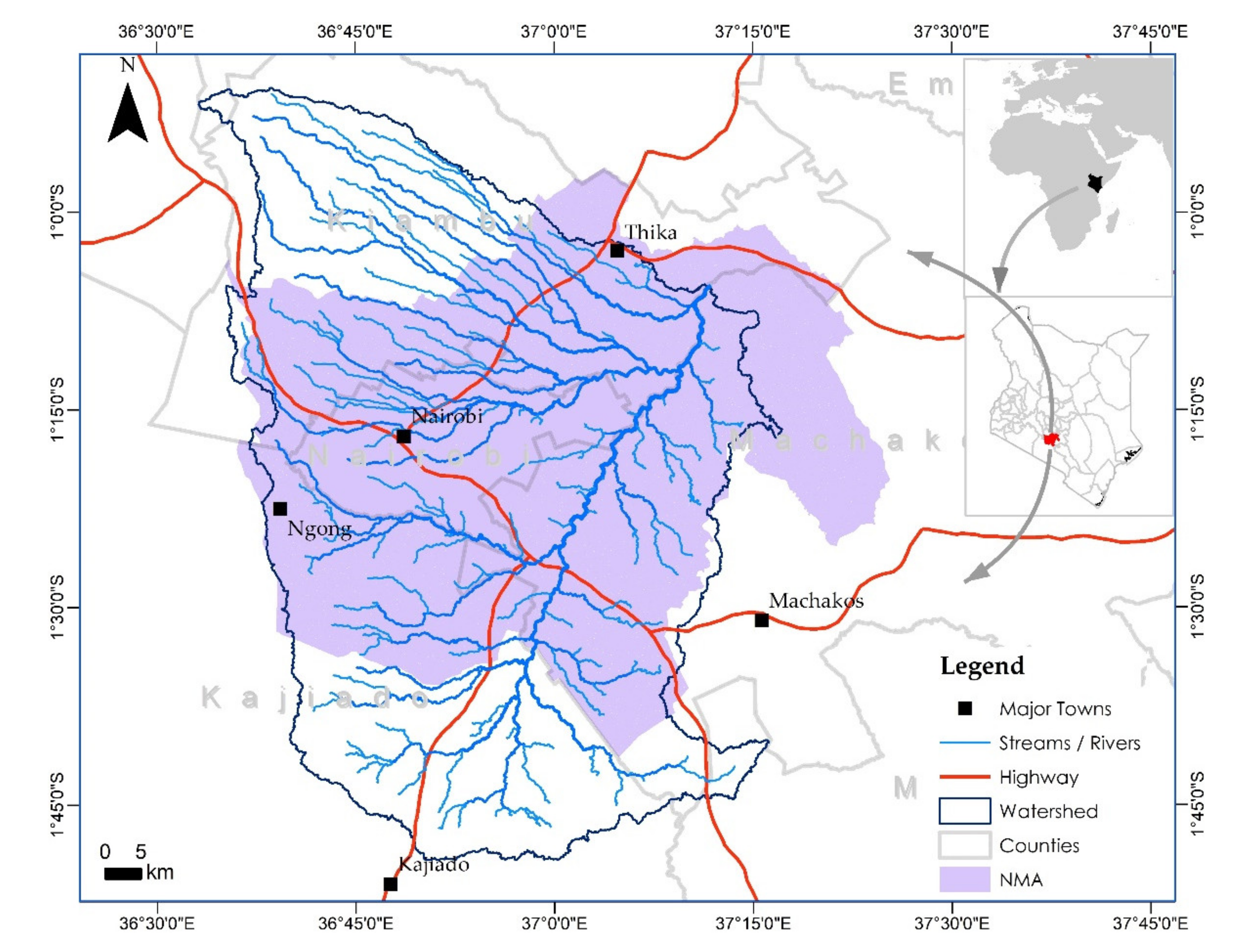
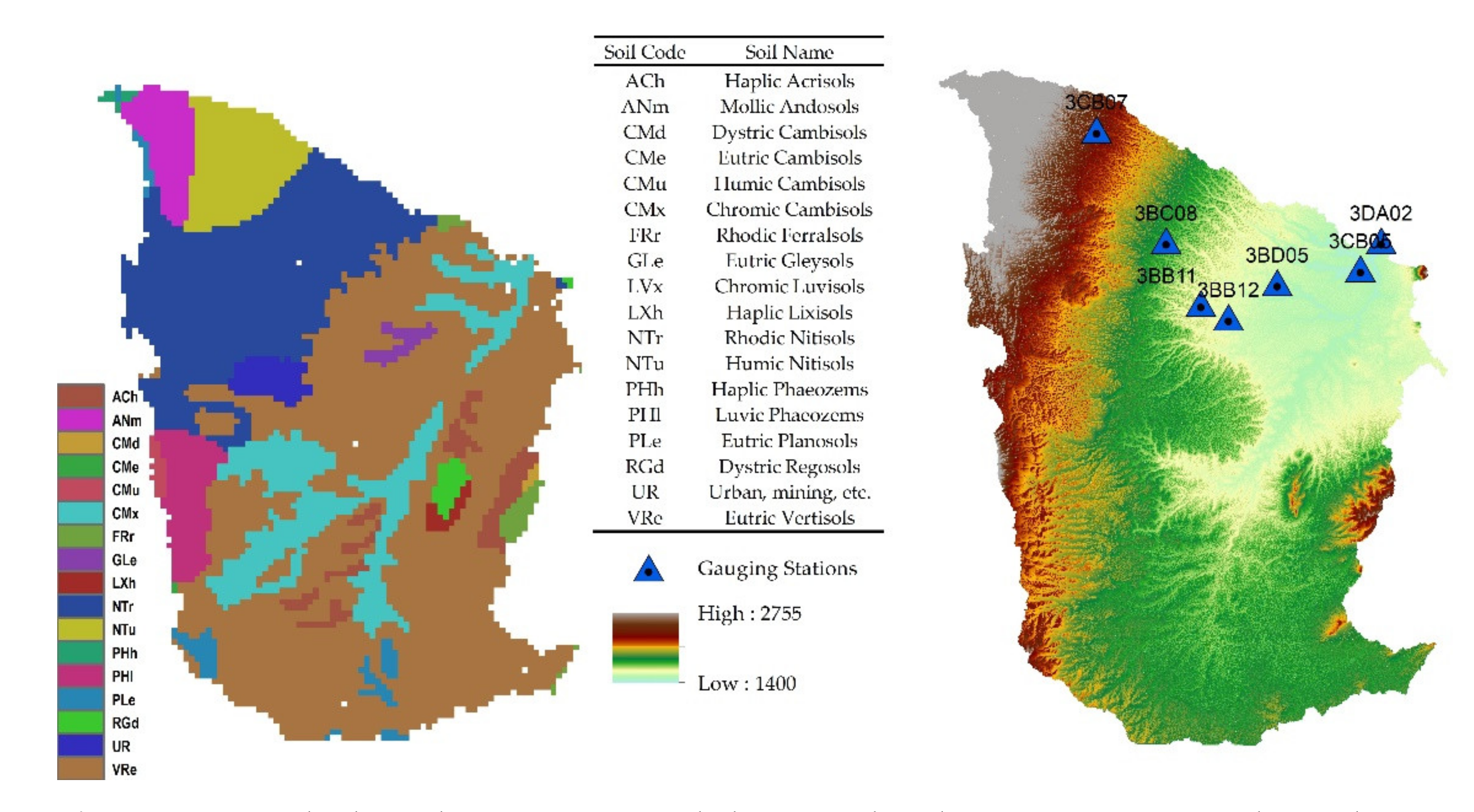
2.1. Study Area

Nairobi metropolitan area (NMA) (Figure 1) is situated in the upper Athi basin lying between latitude 0°45′ S~1°48′ S and longitude 36°30′ E~37°15′ E. The watershed’s topography is characterised by steep ranges in the east and rolling plains to the west. The soil distribution majorly consists of Rhodic Nitisols along the steep volcanic slopes, Cambisols and poorly-drained Eutric Vertisols on the gently undulating western region. The watershed is predominantly agricultural, grasslands and cluster of polycentric urban areas. The climate is warm and temperate, and the annual precipitation during the study period varied from 552 mm to 1620 mm and temperatures above 19.0 °C with the hottest month and the wettest month in February and April, respectively. The watershed experiences two wet seasons, with the significantly wet season in March through April than in October through December.

2.2. Datasets

Digital elevation model (DEM) data, needed to compute the flow accumulation, stream links, and watershed delineation, was obtained from the NASA website at a spatial resolution of 30 m. The soil data were obtained from the Harmonized World Soil Database. Eighteen major soil groups were identified based on FAO/UNESCO—ISRIC classification. The soil attributes prepared in the Harmonized World Soil Database (HWSD) and FAO soil map comprised electrical conductivity (EC), pH, organic carbon and soil texture (%sand, %silt, %clay). However, the SWAT model requires soil depth, bulk density, available water content and hydraulic conductivity for each soil layer. These parameters can be estimated using the pedotransfer functions. The weather input data required for SWAT simulation includes daily rainfall, maximum and minimum temperature, wind speed, relative humidity, and solar insolation. Precipitation and temperature data were obtained from high resolution gridded CHIRPS and CHIRTS datasets. Simultaneously, solar radiation, wind speed, and relative humidity were added from the SWAT global weather database. The gridded data was sampled on 42 stratified random stations to act as station input for the data. The meteorological data used for this study covers 36 years from January 1981 to December 2016. The land-use/land cover maps were classified and validated using image composites in the Google Earth Engine (GEE).

2.3. Land Use Model

The future land use simulation (FLUS) model [66] is a self-adaptive model for land use scenario simulation designed based on the cellular automata (CA) theory and artificial neural networks (ANN). The model is implemented by training an ANN model to generate the urban probability of occurrence by finding complex relationships between land use patterns and the human and natural environment driving factors. The probability of occurrence guides the allocations of land use distribution changes. At the same time, a designed roulette mechanism models urban and non-urban area competition in each cell. The simulation is then forecasted in a tightly coupled “bottom-up” CA model and “top-down” Markov chain model to determine transition probabilities of change from one class to another.

The FLUS model requires two land use maps (one as model input and another for precision and validation), driving factors classified as natural factors and human factors (such as altitude, slope, aspect, proximity to towns, cities, roads, rails), and restriction zones for exclusions (such as water, protected areas and policies) to create the probability of occurrence and perform self-adaptive inertia and competition mechanism. Due to the complex landscape features and vast socio-economic data required to fit various sub-modules and components, FLUS can only execute a single scenario equivalent to the historical trend. Map validation is done using the Kappa statistic and figure of merit (FOM).

FLUS model has been applied successfully both in global and local scales to simulate elaborate land-use/land cover and has seen improvements in the recent past through tailored applications [67,68,69]. It is a powerful tool with diverse applications not limited to establishing urban construction boundaries (UCBs), discriminating large scale LULC, hotspot recognition, land suitability analysis and future land-use simulations.

2.4. Climate Models

Downscaling global climate models (GCMs) provide an effective adaptation strategy to obtain high-resolution future climate simulation at regional and local scales. The approach assumes that large scale weather exerts a significant influence on the local scale. However, it disregards reverse local scale effects. Downscaling can be accomplished in two approaches, i.e., statistical downscaling and dynamic downscaling. Statistical downscaling is developed based on statistical transfer function between local climate observations and the large scale GCM outputs, assuming that the past climate statistics will remain valid in the future. For dynamic downscaling, high-resolution regional climate models (RCMs) is nested within GCM and solved using boundary conditions from the GCM. The assumption is that high-resolution RCM could simulate local climatic conditions over a limited region in greater detail. Statistical downscaling is widely used because it is inexpensive computationally. However, its downscaling skill depends on the predictor stationarity. In this study, dynamic downscaling was selected with an assumption that observed predictor and prediction relationships would remain reasonable under different future climatic forcing conditions.

Regional climate model (RCM) simulations (

Table 1. Regional climate models (RCMs) used in the study. Historical, RCP4.5 and RCP8.5 were obtained from the CORDEX project.

Institute	RCM	Driving GCM	Historical	RCP4.5	RCP8.5
SHMI	RCA4	CNRM-CERFACS-CNRM-CM5	√	√	√
SHMI	RCA4	CSIRO-QCCCE-CSIRO-Mk3-6-0	√	√	√
SHMI	RCA4	MOHC-HadGEM2-ES	√	√	√
SHMI	RCA4	MPI-M-MPI-ESM-LR	√	√	√
SHMI	RCA4	NCC-NorESM1-M	√	√	√
SHMI	RCA4	NOAA-GFDL-GFDL-ESM2M	√	√	√

) from the Coordinated Regional Climate Downscaling Experiment Program (CORDEX) were obtained from the CORDEX Project under the Africa Domain with a spatial resolution of ~50 km (0.44°). Monthly mean precipitation (P_avg), maximum (T_max) and minimum (T_min) surface air temperatures were evaluated against CHIRPS and CHIRTS gridded datasets for model skill and systematic biases using methods put forth by Kim et al. [70]. The RCMs used in this study are based on two representative concentration pathways (RCP) scenarios; the high emission scenario (connoted as RCP8.5) and mid-range mitigation emission (RCP4.5) [71]. RCP4.5 assumes that economic structures are rapidly changing, with the aim of reducing the material intensity and introducing clean energy, with a focus on a global solution to economic, social and environmental stability. In the year 2100, the scenario will stabilise the radiative force at 4.5 W/m² without ever exceeding it. RCP8.5 [72], on the other hand, is a worst-case scenario (the current trend) characterised by high population growth, a lower rate of development of technology, little efforts to curb emissions, and a heavy reliance on coal-fired power [71]. RCP8.5 radiative forcing will peak by 2100 at 8.5 W/m² and overshoot the value due to heavy fossil fuel dependence.

The years 2051–2059 (near future) and 2080–2089 (far future) served as future scenario periods and the period from 1981 to 2016 as a historical baseline to evaluate the climate biases. Other baseline weather variables such as solar radiation, relative moisture and wind speed were omitted in future scenarios as changes in these variables may not significantly affect the local hydrology’s climate simulations [73].

The model’s climatology has been evaluated under four subregions to select the best model having the best model skill with the observations. Four statistical functions are hereby used: Correlation, RMSE, standard deviation and bias.

2.5. Bias Correction

Once the best model was selected, climate model data for hydrological modelling (CMhyd) [74] was used to apply the precipitation and temperature bias correction. While applying five precipitation corrections methods and three temperature correction methods on an arid watershed, Fang et al. [75] noted that power transform (PT) and quantile mapping (QM) performed equally best in fixing precipitation’s frequency-based indices. Simultaneously, local intensity scaling (LOCI) performed best in correcting time series-based indices in precipitation. The three tested correction techniques (linear scaling (LS), variance scaling (VARI), and distribution mapping (DM)) worked relatively the same for temperature correction. While using CMhyd to test five bias correction methods on 12 model combinations, Zhang et al. [76] noted that DM performed best for both precipitation and temperature bias corrections. Owing to the successful application of DM in bias correction of temperature [34] and the need to correct precipitation time-series indices, local intensity scaling (LOCI) was used in precipitation bias correction. In contrast, distribution mapping was used to temperature bias correction of T_max and T_min.

2.6. QSWAT Interface

QSWAT can be divided into two sections: (1) A QSWAT Control containing the code that responds to the user’s interactive input; and (2) QSWAT functions housing the code to implement specific tasks such as combining sub-basins or snapping points to a stream link [53]. It depends on a set of programs termed terrain analysis using digital elevation models (TauDEM, http://hydrology.usu.edu/tandem/taudem5; accessed on 17 November 2020) to execute several geoprocessing functions combined with QGIS inbuilt functions. QSWAT accepts GDAL supported rasters and vectors. It creates copies in the project directory linked using relative paths, making it easy to move, copy, or archive projects between and within computers.

During model execution, QSWAT first performs watershed delineation using TauDEM by executing functions such as pit (depression) removal, calculation of contributing areas, delineation of stream networks, watersheds and sub-basins, routing to stream sections and linking subbasin and stream segment attributes. Secondly, it creates homogenous HRUs using the intersection of land use, soil maps and related lookup tables. Each HRU will belong to a particular sub-basin, and each cell has the same land use, soil layer, and slope range. Thirdly, QSWAT is then linked with SWAT Editor to create several database tables from the previous two steps. SWAT Editor will help create or import weather databases, edit control databases, execute the SWAT model, manually calibrate outputs, and export SWAT outputs. Lastly, QSWAT enables three visualisations for investigation and analysis in the QGIS map window: static, dynamic and plot function. Static and dynamic visualisations are designed to show spatial distribution through symbology or the creation of categorical displays, with dynamic visualisation encapsulating time steps. The plot function displays graphical outputs for comparisons read using a separate tool called SWATGraph. The graphs can be exported as a comma-separated value (CSV) file. Further, SWATGraph can calculate the correlation coefficient (R) and Nash–Sutcliffe efficiency (NSE) coefficients between simulated and observed data.

2.7. Model Setup

A 30 m spatial resolution DEM was used to generate a stream network. Hydrological station 3DA02 (Figure 2) was considered an outlet point to offer a threshold value to delineate the watershed boundary. A prepared land use containing six classes, soil map and its respective lookup tables, and slope map (classified into five slope classes) was subjected to a defined threshold of 10% land use, 20% soil and 10% slope as put forth by Setegn et al. [77] delineating 23,699 valid HRUs. SWAT uses Soil Conservation Service’s curve number (CN) method for runoff estimation. The Penman–Monteith method and variable storage routing method are used to estimate potential evapotranspiration and flow routing respectively.

The SCS-CN model can be expressed in its general form as follows:

$$Q=\frac{{\left(P-I_{\alpha }\right)}^2}{P-I_{\alpha }+S},I_{\alpha }=\lambda S$$

(1)

where $P$ is the total precipitation (mm), $I_{\alpha }$ is the initial abstraction (mm), Q is the direct surface runoff (mm), S is the potential maximum retention (mm) after runoff begins, and $I$ is the initial abstraction coefficient. When $I_{\alpha }$ is taken to be 0.2 S, i.e., $I_{\alpha }=0.2$ Equation (3) becomes:

$$Q=\frac{{\left(P-0·2S\right)}^2}{P+0·8S} for P>0 else Q=0$$

(2)

S can be converted into a unitless CN, variable in a logical scale (0, 100) and can be stated as:

$$S=\frac{\mathrm{25,400}}{CN}-254$$

(3)

The CN values were obtained from the intersection of watershed characteristics (land use land cover, soil hydrologic condition, hydrologic soil group and antecedent soil moisture condition) [78]. These equations take into account the watershed characteristics in the form of S and the effect of rainfall variation.

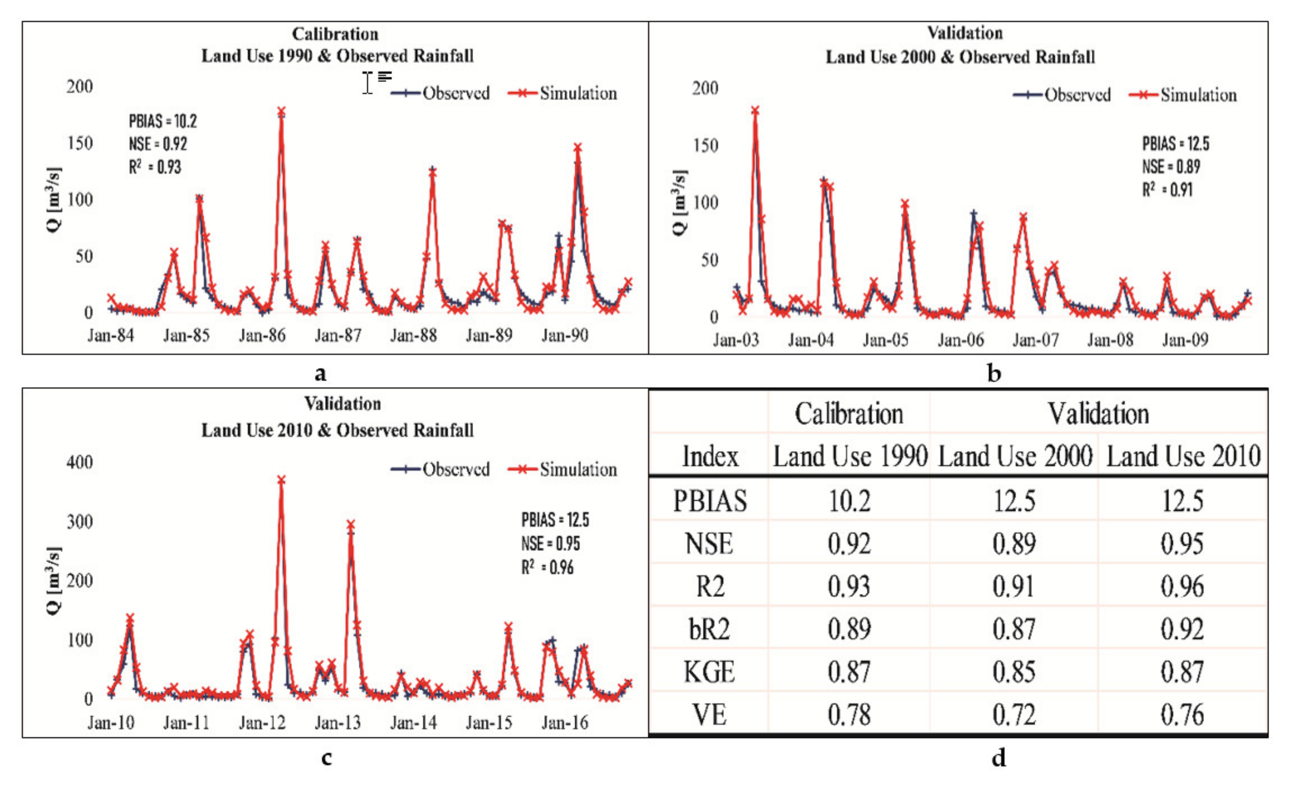
2.8. Sensitivity Analysis, Calibration and Validation

For optimal model performance, surface runoff, subsurface flow, and temporal flow must be calibrated. Sequential Uncertainty Fitting version 2 (SUFI-2) algorithm [43] has been widely used for automatic calibration and sensitivity analysis of SWAT models. QSWAT, however, can be calibrated using: (1) SWATCup-plus SUFI-2, a premium version of the public domain SWAT-CUP; (2) a novel Integrated Parameter Estimation and Uncertainty Analysis Tool Plus (IPEAT+) [79] explicitly designed for SWAT+; and (3) inbuilt SWAT Editor hard and soft calibration. In this study, sensitivity analysis and calibration were performed in two phases: first, sensitive model parameters from

Table 2. SWAT+ calibration parameters. Default values obtained from the calibration parameters file.

Parameter	Object Type	Description	Range
cn2	hru	Initial SCS runoff curve number for moisture condition II.	28–98
awc	sol	Available water content of the soil layer (mm H2O/mm).	0.01–1.0
esco		Soil evaporation compensation factor.	0.01–1.00
perco	hru	Amount of water percolating out of root zone (mm H2O)	0–1
gw_lte	hlt	Initial shallow aquifer storage	0–10 m
revap_co	aqu	Groundwater “revap” coefficient.	0.02–0.2
revap_min	aqu	Minimum depth of water in the shallow aquifer for percolation to the deep aquifer to occur (mm H2O).	0–10 m
alpha_bf	aqu	Baseflow alpha-factor (days).	0–1 day
canmax	hru	Maximum canopy storage (mm H2O)	0–100 mm/H2O
k_ch	rte	Effective hydraulic conductivity in tributary channelalluvium (mm/h).	0–0.01–500 mm/h
flo_min	aqu	Minimum water depth in the shallow aquifer required to return flow (mm H2O).	0–10 m
gwflow	lte	Groundwater contribution to streamflow (mm H2O).	0–10 m
gwdeep	lte	Deep aquifer percolation fraction.	0–10 m
ovn	hru	Manning’s “n” value for overland flow	0.01–30

were identified using relative sensitivity analysis suggested by Haan [80], and then calibration was done using IPEAT+ after identifying the sensitive parameters. IPEAT+ is freely available while SWATCup plus requires a license to calibrate SWAT+ model data. SWAT+ is incompatible with the public domain SWATCup.

Based on previous studies, fourteen most influential parameters were selected for analysis using the relative sensitivity analysis method proposed by Haan [80] as follows:

$$S_r=\frac{\left[\frac{O_{P+\Delta P} - O_{P-\Delta P}}{O_P}\right]}{\left[\frac{2\Delta P}{P}\right]}$$

(4)

where S_r is the relative sensitivity, $O_{P+\Delta P}$ is the model outputs with the input parameter set at the base value plus a specified percentage (between 10 and 25%), $O_{P-\Delta P}$ is the model outputs with the input parameter set at base minus a specified percentage (between 10 and 25%), $O_P$ is the model output with input parameter set at the base value $\Delta P$ is the prescribed input parameter absolute change value, and p is the initial input parameter base value.

Regarding the absolute value of $\Delta P$, Lenhart et al. [81] found out that varying value by 25% gave a more contrasted outcome than when as low as 10%. Other studies have successfully used ±25% as the variation value [82,83]; therefore, $\Delta P\pm 25\%$ of was taken as the absolute variation for the study sensitivity test. Mean relative sensitivity ($\mu S_r$) parameter values were then classified into four sensitivity categories as defined by Lenhart et al. [81] (

Table 3. Mean relative sensitivity categories for classifying the parameter sensitivity.

Class	$\mathit{\mu }{\mathit{S}}_{\mathit{r}}$	Sensitivity Category
I	0.00 ≤ $\mu S_r$ < 0.05	Small to negligible
II	0.05 ≤ $\mu S_r$ < 0.20	Medium
III	0.2 ≤ $\mu S_r$ < 1	High
IV	$\mu S_r$ > 1	Very high

).

After the completing sensitivity analysis, the three primary IPEAT+ controls files, i.e., the technical control file (IPEAT_Control.set), the parameter setting file (IPEAT_para.set) and the observation file (IPEAT_ObsXY.set) were set. IPEAT_Control.set contains variables needed to conduct the optimisation algorithm and define the calibration variables, including objective functions. IPEAT_para.set defines the full list of candidate parameters available for calibration in SWAT+, which is the same as that cal_parms.cal in the SWAT model, while IPEAT_ObsXY.set defines the simulation timestep (day, month, or year), the outlet number to be calibrated, and the observations used in model calibration. Monthly streamflow was examined, and five statistical goodness-of-fit indices (

Table 4. Statistical goodness-of-fit indices to probe model validity.

Coefficient	Description	Optimal Values
Percent bias (PBIAS) [85]	measures the average tendency of the simulated channel flow to deviate from the observed flow.	0—Optimal, Negative—underestimation, Positive—overestimation
Nash-Sutcliffe efficiency (NSE) [86]	a normalised statistic that calculates the relative magnitude of the simulated flow variance compared to the observed flow variance.	NSE = 1 perfect match, NSE = 0, model predictions accurate as the mean of the observed data, -Inf < NSE < 0, observed mean is a better predictor than the model
Product of coefficient of determination (R2) and the regression line slope between simulation and observation (bR2) [87]	allows measurement for the discrepancy in the magnitude of simulated and observed flows (b) and their dynamics (R2)	0 ≤ bR2 ≤ 1 1—Optimal, >0.5—good match, <0.5—representative.
Kling-Gupta efficiency (KGE) [88]	aids the evaluation of the relative importance of diverse components (correlation, bias, and variability)	-inf < KGE > 1 $~1$ efficient
Volumetric efficiency (VE) [89]	represents the fraction of water reaching the channel at the proper time	-Inf ≤ VE ≤ 1 $~1-$ efficient

) were calculated in the R software using the hydroGOF library [84] as the model performance indicators.

$$PBIAS=\frac{{{\displaystyle \sum }}_{i=1}^n\left(Y_i^{obs}-Y_i^{sim}\right)}{{{\displaystyle \sum }}_{i=1}^n\left(Y_i^{sim}\right)}·100$$

(5)

$$NSE=1-\frac{{{\displaystyle \sum }}_{i=1}^n{\left(Y_i^{obs}-Y_i^{sim}\right)}^2}{{{\displaystyle \sum }}_{i=1}^n{\left(Y_i^{obs}-Y_{obs}^{mean}\right)}^2}$$

(6)

$$b{R}^2={\left(\frac{{{\displaystyle \sum }}_{i=1}^n\left(Y_i^{obs}-Y_{obs}^{mean}\right)\left(Y_i^{sim}-Y_{sim}^{mean}\right)}{\sqrt{{{\displaystyle \sum }}_{i=1}^n{\left(Y_i^{obs}-Y_{obs}^{mean}\right)}^2}\sqrt{{{\displaystyle \sum }}_{i=1}^n\left(Y_i^{sim}-Y_{sim}^{mean}\right){ }^2}}\right)}^2$$

(7)

$$KGE=1-\sqrt{{\left(r-1\right)}^2+{\left(\beta -1\right)}^2+{\left(\gamma -1\right)}^2}$$

(8)

$$VE=1-\frac{{{\displaystyle \sum }}_{i=1}^n\left|Y_{sim}-Y_{obs}\right|}{{{\displaystyle \sum }}_{i=1}^n{Y}_{obs}}$$

(9)

where Y is the streamflow discharge, obs is the observation, while sim is the simulation. r is the correlation coefficient, $\beta$ is the bias ratio (dimensionless) and $\gamma$ is the variability ratio (dimensionless)

Three historical epochs were selected for calibration and validation. Due to gaps in the hydrological station data, 1984–1990 was selected as base years for calibration using corresponding historical meteorological data and the year 1990 land use map. For validation, the land use map for the year 2000 was validated using 2003–2009 weather data. The land use map for the year 2010 was validated using 2010–2016 weather data. All simulations had an initial one year warming period, i.e., 1983, 2002 and 2009.

2.9. Evaluation of the Effects of LULC and Climate Change on Surface Runoff

To assess impacts of LULC and climate change on the surface runoff, runoff discrepancies have been evaluated annually in three phases: (1) The impacts of LULC is independently evaluated using historical data and assuming that the observed historical meteorological data are subject to negligible climate change effects; (2) the independent climate influence is tested by changing meteorological conditions over a static 2010 land use map; and (3) the combined effects of LULC and climate change are evaluated using future corrected climate data and projected land use evolution. Under the first condition, 1984–1990 serves as a baseline for 2003–2009 and 2010–2016 LULC scenarios. For the third condition, two bias-corrected RCM data under RCP4.5 and RCP8.5 were combined with the historical trend of LULC and evaluated under three temporal conditions at 30-year interval; historical baseline (2010s), near future (2050s), and far future (2080s). This temporal spacing is likely to enable climate change effects to be pronounced as the climate is considered at least a 30-year weather average.

The deviation from baseline observation of two SCS-CN model variables (the runoff depth (Q) and runoff coefficient (α)) were evaluated to assess land use and climate impacts on the surface runoff as given below:

$$\Delta Q=Q_a-Q_b$$

(10)

$$\propto =\frac{Q}{P},\Delta \propto =\frac{\Delta Q}{P}$$

(11)

$$\beta =\frac{Q_{i+1}-Q_i}{Q_i}$$

(12)

where $Q_a$ and $Q_b$ denotes surface runoff depths (mm) of the baseline and the subsequent land-use scenarios, respectively, $P$ is the rainfall depth (mm), $\Delta Q$ is the change in runoff depth between two successive epochs, $\Delta \propto$ is the absolute change in the runoff coefficient and $\beta$ represent the relative degree of change between to subsequent land use/climate scenarios ($i$). Positive values of $\Delta Q$ and $\Delta \propto$ indicate land use/climate change increased the surface runoff, reduced if negative, or otherwise, no significant changes [90].

3. Results and Discussion

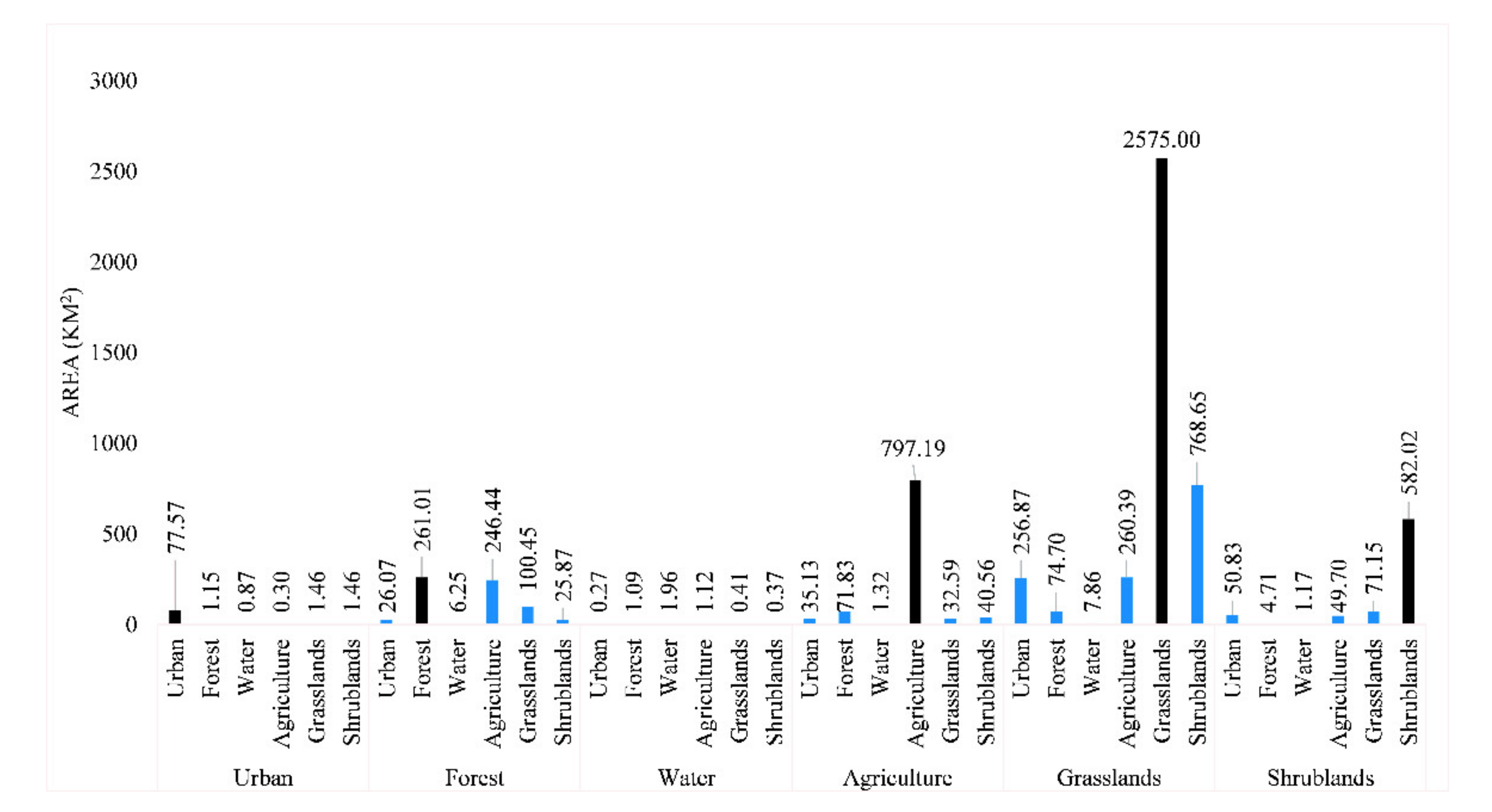
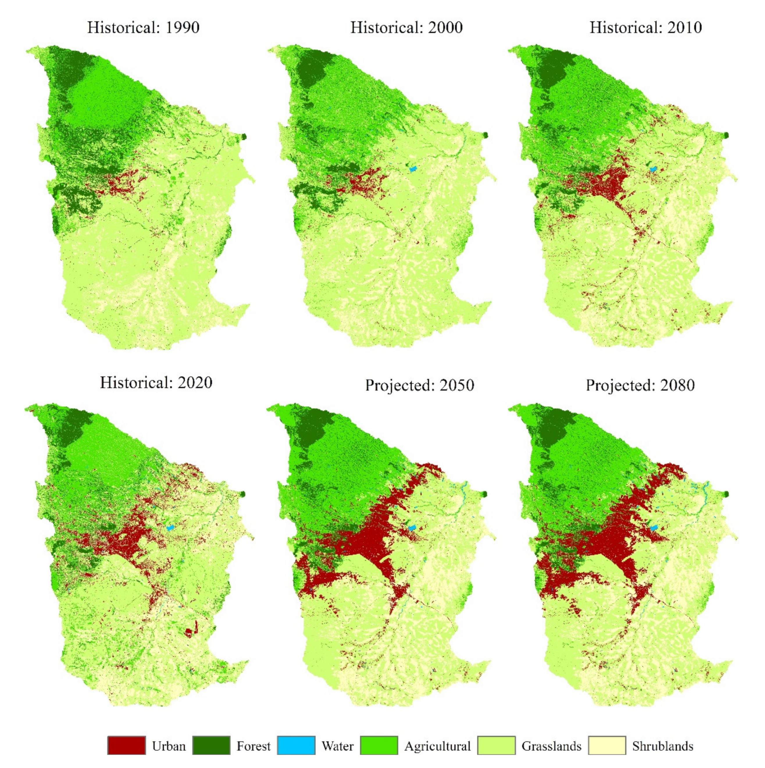
3.1. Land Use/Land Cover Change Analysis

A confusion matrix is used to establish the correctness of the classified image during the accuracy assessment. Randomly-selected points were compared to the classification maps from the image mosaics and the Google Earth image as a reference. 301, 576, 1020 and 1407 sampling points were chosen to validate images from 1990, 2000, 2010 and 2020. Results (

Table A1. Confusion matrix, 1990.

1990
	URB	FOR	WAT	AGR	GRA	SHR	Total	U_Accuracy	Kappa
URB	50	0	0	0	0	0	50	1
FOR	0	64	1	2	2	0	69	0.93
WAT	0	0	9	0	0	0	9	1
AGR	0	3	0	51	5	0	59	0.86
GRA	0	1	0	0	46	5	52	0.88
SHR	6	0	0	7	7	42	62	0.68
Total	56	68	10	60	60	47	301
P_Accuracy	0.89	0.94	0.90	0.85	0.77	0.89		0.87
Kappa									0.84

,

Table A2. Confusion matrix, 2000.

2000
	URB	FOR	WAT	AGR	GRA	SHR	Total	U_Accuracy	Kappa
URB	81	0	0	0	0	0	81	1.00
FOR	0	87	4	5	0	0	96	0.91
WAT	0	0	31	0	0	0	31	1.00
AGR	1	10	0	131	2	0	144	0.91
GRA	9	3	0	10	110	8	140	0.79
SHR	3	0	0	2	7	72	84	0.86
Total	94	100	35	148	119	80	576
P_Accuracy	0.86	0.87	0.89	0.89	0.92	0.90		0.89
Kappa									0.86

,

Table A3. Confusion matrix, 2010.

2010
	URB	FOR	WAT	AGR	GRA	SHR	Total	U_Accuracy	Kappa
URB	171	0	1	2	2	0	176	0.97
FOR	0	174	2	30	0	0	180	0.97
WAT	3	0	71	0	0	0	74	0.96
AGR	4	3	0	296	0	0	303	0.98
GRA	0	1	2	9	169	7	188	0.90
SHR	6	0	0	1	8	84	99	0.85
Total	184	178	76	312	179	91	1020
P_Accuracy	0.93	0.98	0.93	0.95	0.94	0.92		0.95
Kappa									0.93

and

Table A4. Confusion matrix, 2020.

2020
	URB	FOR	WAT	AGR	GRA	SHR	Total	U_Accuracy	Kappa
URB	301	0	0	15	2	0	318	0.95
FOR	0	379	2	3	1	0	385	0.98
WAT	0	0	101	0	0	0	101	1.00
AGR	0	3	5	367	6	3	384	0.95
GRA	1	1	2	6	82	7	99	0.83
SHR	2	0	0	9	5	104	120	0.87
Total	304	383	110	400	96	114	1407
P_Accuracy	0.99	0.99	0.92	0.92	0.85	0.91		0.95
Kappa									0.93

) reveal that the average precision for 1990, 2000, 2010 and 2020 maps was 87%, 89%, 95% and 95%, respectively. The producer’s accuracy ranged from 85% to 99%, while the user’s accuracy ranged from 79% to 100%.

For the predicted land use map, 5% of the valid pixels (

Table A5. 5% valid cells samples for validating predicted land use map, 2020.

Land Use Types	Urban	Forest	Water	Agricultural	Grassland	Shrubland	Total
Urban	22563	24	107	1843	1265	95	25897
Forest	76	32402	18	4468	881	0	37845
Water	8	0	409	0	7	0	424
Agricultural	781	372	77	76073	22090	49	99442
Grassland	3478	11	108	12537	176014	361	192509
Shrubland	114	0	0	260	9323	77019	86716
Total	27020	32809	719	95181	220324	77524	453577

in Appendix B) in the 2020 predicted raster were randomly selected to compute the confusion matrix against the 2020 classified image (ground truth). The overall accuracy was 88%, and the Kappa statistic was 0.84 (

Table A6. Accuracy assessment of the predicted land use map, 2020.

Land Use Types	Commission Error	Omission Error	Producer’s Accuracy	User’s Accuracy
Urban	0.13	0.16	0.84	0.87
Forest	0.14	0.01	0.99	0.86
Water	0.04	0.43	0.57	0.96
Agricultural	0.24	0.20	0.80	0.76
Grassland	0.09	0.20	0.80	0.91
Shrubland	0.11	0.01	0.99	0.89
Kappa	0.835048		Overall	0.8750

). Commission errors were high in agricultural land use (0.24), while the omission errors were high in the water land class (0.43). Additionally, the computed figure of merit (FoM) was 23.43%. Similar studies computed FoM values ranging from 12% to 59% [66,91,92]. Low FoM can be attributed to the short simulation period used in the study (2010–2020), as long-term simulations have relatively higher FoM values [66,91].

Historical land use/land cover change (

Table 5. Historical and future land use composition in the watershed.

	Urban	Forest	Water	Agriculture	Grasslands	Shrublands
1990	85.87	666.01	5.93	980.90	3162.12	785.02
2000	98.73	401.99	10.78	1041.76	3097.78	1034.78
2010	274.98	427.09	9.64	1083.75	2817.02	1073.40
2020	428.31	410.72	19.68	1154.78	2532.13	1140.26
2050	624.58	419.05	21.03	1185.73	2244.61	1190.17
2080	725.20	392.75	23.27	1194.67	2169.12	1181.17

) between 1990 and 2020 was dominated by the change in the grasslands (σ = 423.71) with a total loss of 629.99 km² followed by urban (+342.44 km², σ = 267.46) and shrublands (+355.24 km², σ = 151.11). Agricultural land showed an increasing trend gaining 173.88 km² (σ = 85.87) while water changed the least (+13.75 km², σ = 7.15).

For the class-to-class transitions (Figure 3), grasslands loss made it the primary player in the watershed. About 768.65 km² of grasslands in 1990 have transited to shrublands gaining about 71.15 km² with a net loss of −697.5 km² between these two classes. Additionally, much of its area has been converted to agricultural (505.83 km²), urban (373.28 km²) and forest (166.04 km²). Forest also has seen a decrease in its coverage (net −405.08 km²), chiefly lost to agricultural (246.44 km²), cleared to grassland-like land (100.45 km²), and urban (26.07 km²). However, it has reclaimed a substantial 152.39 km², mostly from grasslands (74.70 km²), agricultural (71.83 km²) and shrubs (4.71 km²).

Projected land use land cover (Figure 4) based on the recent land-use transition probabilities (between 2010 and 2020) instead of long-term land-use trends (1990–2020) has been used to capture current land-use dynamics. It was noted that high class to class transition probabilities between 1990 and 2020 land use maps did not accurately reflect current trends in urban and forest land utilisation as compared to using recent land-use epochs. This was partly because the CA-Markov land use prediction only considers two sets of land use maps for LULC simulation. Urban land cover is expected to rise steadily to about 624.58 km² in 2050 and 725.20 km² in 2080, an equivalent of 45.82% increase between 2020 and 2050 and a 16.11% increase between 2050 and 2080. Agricultural land, shrubland and water land use land cover classes exhibit positive net change. At the same time, forest and grasslands will continue to be converted to other land uses. The loss of grasslands could be attributed to the urban growth in the suburbs in the Kajiado, Kiambu and Machakos counties. Increasing agricultural land demand would likely absorb significant portions of the forests.

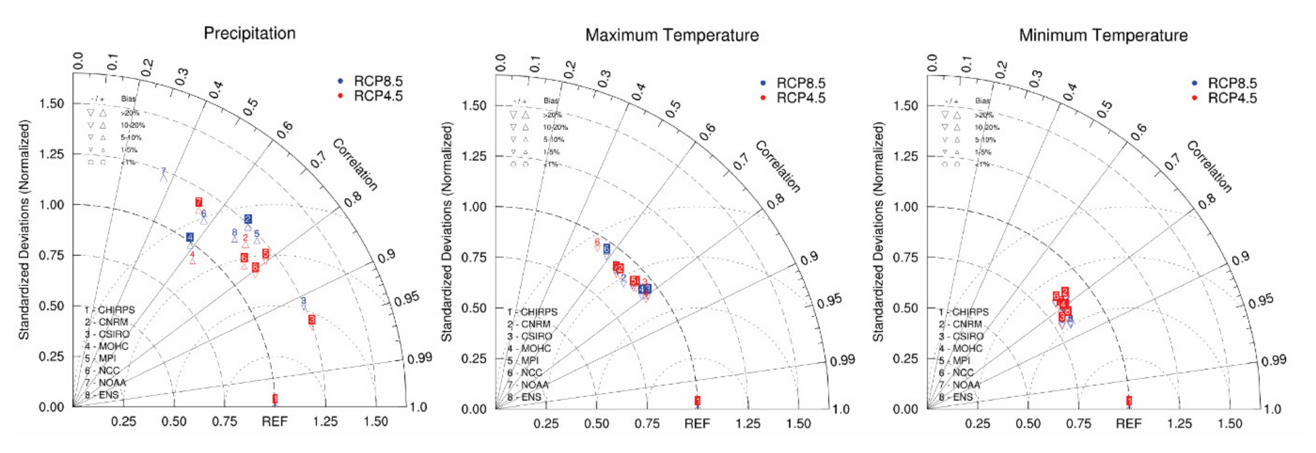
3.2. Climate Data Evaluation

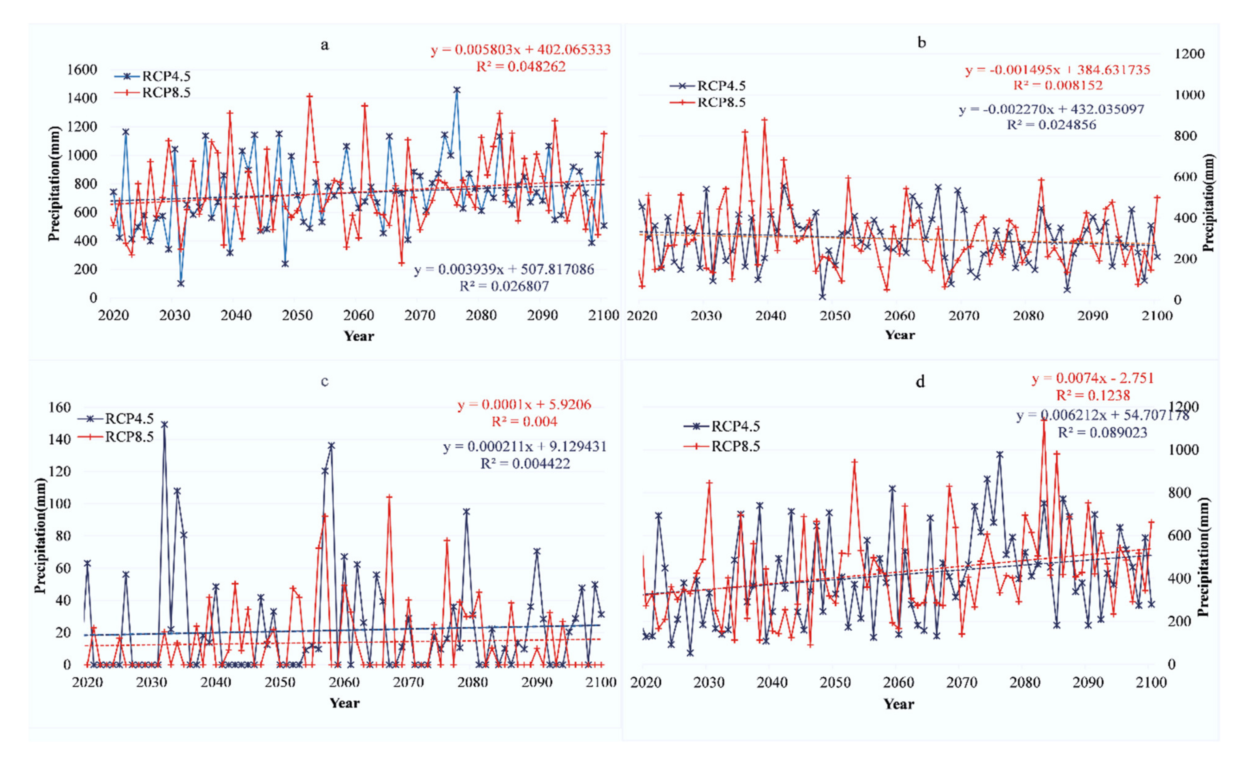
3.2.1. Precipitation

All the precipitation RCMs generated wet biases in the wettest northern region and dry biases in the study area’s southern region. Among the models, CSIRO and the ensemble (ENS) performed best with high spatial correlation (R > 0.8) for RCP4.5. However, ENS dropped in quality under RCP8.5 (R > 0.7). Additionally, comparing all models, CSIRO yielded the lowest RMSE (<10%) followed by the ENS, whereas NOAA yielded the highest (>20%) in both climate scenarios. NOOA, MOHC and ENS had the lowest standard deviation against CHIRPS data. On evaluating model skill (spatial correlation, biases, RMSE, and standard deviation), CSIRO and ENS performed better under both climate scenarios in the study area, with CSIRO being selected for statistical downscaling (Figure 5).

Corrected precipitation (Figure 6) exhibits an increasing annual precipitation trend from 2021 to about 2076 in both climate scenarios. These findings show consistency with other previous studies considering rainfall projections in East Africa [93]. However, long rains (March–April–May, (MAM)) are set to decline while short rains (ON and DJF) are expected to increase. The cause of these seasonal variabilities is still debated. Williams et al. [94] attributed these changes to the enhanced convection in the Western Equatorial Pacific stretching warm pool and Walker circulation towards the Indian ocean. In contrast, Lyon et al. [95] linked the decline to the warming SSTs over the Western Tropical Pacific and the cooling SSTs over the Eastern Tropical Pacific. The linear rainfall trend is not determinant; hence, it is inaccurate to estimate linear annual average precipitation change. Generally, the results suppose an annual loss of 3 mm of precipitation in the MAM season and an annual net gain of 0.2 mm and 14 mm in JJAS and ONDJF, respectively.

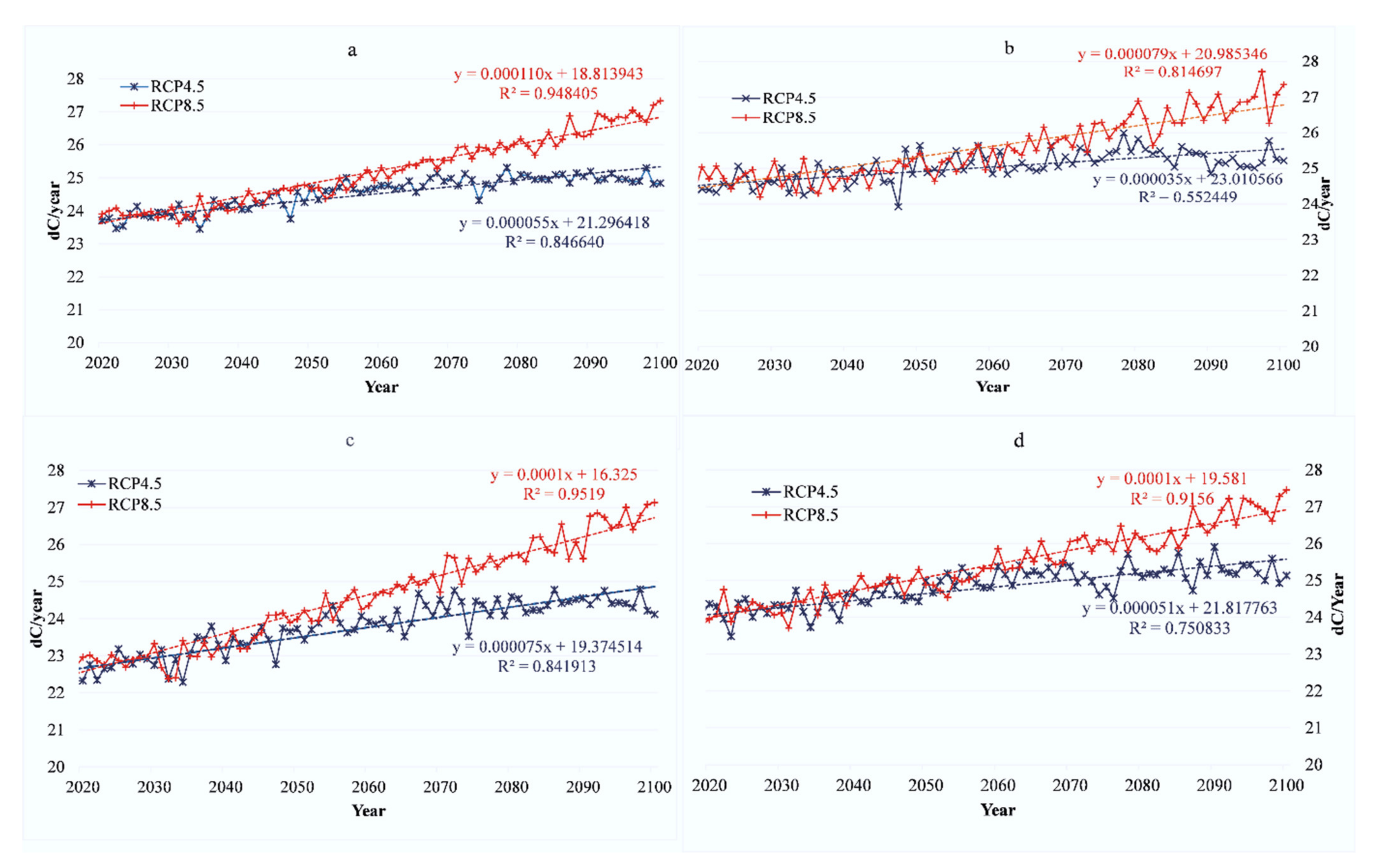
3.2.2. Surface Air Temperature

T_max and T_min evaluation were also performed against CHIRTS data, with all the models underestimating both T_max and T_min. Under both climate scenarios, T_max spatial correlation ranged from 0.55 to 0.82, while all models yielded almost a unified spatial correlation for T_min ranging from 0.8 to 0.85. ENS (bias < 20%, 1.02 < RMSE < 1.75) and CSIRO (bias < 20%, 1.02 < RMSE < 1.61) performed best for T_min under both climatic scenarios, while CSIRO (bias < 20%, 0.71 < RMSE < 0.87) and MOHC (bias < 20%, 0.51 < RMSE < 0.65) had a good skill for estimating T_max. In the light of the CSIRO model’s high performance for precipitation and surface air temperatures and the efficiency in single model bias correction, CSIRO-QCCCE-CSIRO-Mk3-6-0 driven RCM was selected as a representative of future climate data for subsequent bias correction. The CSIRO Mk3.6.0 has also been noted to be the only model to account for both East Africa long rains rainfall-SST relationship and the precipitation climatology [96].

Corrected temperature projections (Figure 7) predict general increase warming at all seasons in the study area, with average increases of about 1.3–1.5 °C under RCP4.5 and about 2.6–3.5 °C under RCP8.5. These findings are consistent with similar studies downscaling RCMs and within limits of the theoretical values [34]. Using 11 RCMs to assess climate change implications on Nile basin water resources, Beyene et al. [97] noted an annual average increase in temperatures ranging from 1.5 °C to 4.4 °C as compared to the historical observations. Under RCP4.5, mean annual temperatures are projected to increase by 0.57 °C, 0.76 °C, and 0.17 °C between 2021–2050, 2050–2080 and 2080–2100. For RCP8.5, mean temperatures will increase by 0.62 °C, 1.21 °C and 0.97 °C under the same periods. Cumulatively, mean temperatures would rise from historical 23.45 °C (2006–2020) to 24.96 °C (+1.51 °C) by 2100 under RCP4.5 and 26.26 °C (+2.81 °C) under RCP8.5 in the NMA.

3.3. SWAT + Model Sensitivity Evaluation

Fourteen SWAT+ parameters (Table 2) were evaluated for sensitivity using relative sensitivity analysis to identify and optimise the three SWAT+ water balance components (total water yield, baseflow, and surface runoff). Four parameters were significantly sensitive to variations and were ranked based on their absolute mean, as tabulated in Table 3. CN2 was the most sensitive parameter to total water yield ($S_r=1.53$), baseflow ($S_r=-1.32$) and surface runoff ($S_r=5.01$) yield. $S_r \mathrm{means}$ that a 1% change in the parameter results in $S_r\%$ change in the affected parameter, i.e., a 1% change in CN2 results in the 1.53% change in the total water yield. Total water yield is sensitive primarily to CN2 ($S_r=1.53$) and SOL_AWC ($S_r=$ −0.31) and mildly to ESCO ($S_r=0.1$) and PERCO ($S_r=-0.03$). Baseflow is affected chiefly by CN2 ($S_r=-1.32)$ and SOL_AWC ($S_r=-0.55)$ with effects of SOL_AWC more pronounced in baseflow balance than in the total water yield. Surface runoff is the most affected parameter by CN2 ($S_r=5.01)$ and also significantly by SOLW_AWC ($S_r=-0.67)$ and ESCO ($S_r=0.11).$ Ranking these parameters (

Table 6. Calibration parameters sensitivity, rank and final calibrated values.

Parameter	Water Yield	Baseflow	Surface Runoff	Sr	Sensitivity Category	Final Calibrated Value	Rank
cn2	1.53	−1.32	5.01	1.74	IV	20.175–79.086	1
awc	−0.31	−0.55	−0.67	0.51	III	0.733	2
esco	0.10	0.09	0.11	0.10	II	0.659	3
perco	−0.03	−0.02	−0.04	0.03	I	0.128	4
gw_lte	0.00	0.00	0.00	0.00	I	-	-
revap_co	0.00	0.00	0.00	0.00	I	-	-
revap_min	0.00	0.00	0.00	0.00	I	-	-
alpha_bf	0.00	0.00	0.00	0.00	I	-	-
canmax	0.00	0.00	0.00	0.00	I	-	-
k_ch	0.00	0.00	0.00	0.00	I	-	-
flo_min	0.00	0.00	0.00	0.00	I	-	-
gwflow	0.00	0.00	0.00	0.00	I	-	-
gwdeep	0.00	0.00	0.00	0.00	I	-	-
ovn	0.00	0.00	0.00	0.00	I	-	-

), CN2 is the most sensitive parameter, followed by SOL_AWC, ESCO, and lastly PERCO.

The four sensitive parameters were calibrated using IPEAT+. A 100 simulation runs were set, and the objective function $1-R^2$ was used to measure and track model performance. It was noted that the model iterations exhibited no further change in parameter randomisation after 59 iterations with optimal objective function $1-R^2$ converging at 0.0657 ($R^2=0.93$). Final optimal values were then used for hard calibration in SWAT Editor for all the subsequent model experiments (land use maps 2000, 2010, 2050, 2080). Both calibration and validation results indicated a good agreement between simulated streamflow and the observed flow data, as tabulated in Figure 8d.

The model success to predict monthly flow with high accuracy reflects CHIRPS and CHIRTS algorithms success in blending CHIRP/CHIRT and station data. Although there is an overestimation of streamflow, monthly flow statistics indicate a good relationship between observed and simulate streamflow. NSE coefficients were 0.92 for the calibration period and 0.89 and 0.95 for the validation periods. A better predictor for estimating volumetric efficiency, the VE, returned satisfactory indices of 0.78, 0.72 and 0.76 during the same phases.

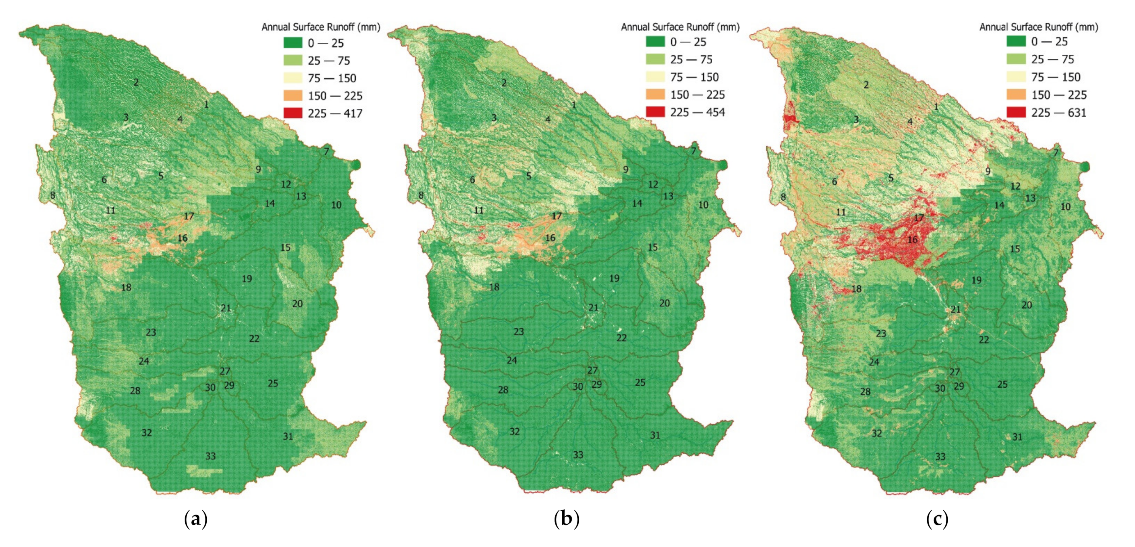
3.4. Surface Runoff Response

3.4.1. Due to LULC

Historical LULCs exhibit a high relationship with the surface runoff response with a statistically insignificant (p > 0.05) correlation with all land classes having a Pearson’s product-moment correlation coefficient ranging from 0.57 to 0.99, as shown in

Table 7. Historical land use relationship with watersheds average surface runoff depth. t—t-statistic, p—p-value, and R²—the Spearman correlation coefficient. Areas in square kilometres.

	Urban	Forest	Water	Agriculture	Grasslands	Shrublands	Q
1990	85.87	666.01	5.93	980.90	3162.12	785.02	18.32
2000	98.73	401.99	10.78	1041.76	3097.78	1034.78	25.32
2010	274.98	427.09	9.64	1083.75	2817.02	1073.40	40.70
t	3.92	−0.93	0.70	3.03	−7.40	1.42	-
p	0.16	0.52	0.61	0.20	0.09	0.39	-
R2	0.94	0.46	0.33	0.90	0.98	0.67	-

. Grasslands $R^2=0.98$, urban land ($R^2=0.94$) classes and agriculture ($R^2=0.90$) are the most contributors to changes in the runoff depth. An increase in urban land and agricultural use corresponded to the increasing surface runoff depth, while the decrease in grasslands corresponded to the increasing surface runoff (Figure 9). Additionally, a decrease in forest cover contributed significantly to the increasing runoff depth ($R^2=0.463$). In contrast, an increase in shrubland cover contributed positively to the average runoff depth ($R^2=0.67)$ whereas water coverage had little relationship with increasing runoff depth.

The average annual runoff depth in the period 2000–2009 (25.32 mm) increased by 38.18% compared to the period 1984–1990 (18.32 mm) supplemented by the increase in urban land use (14.97%), shrublands (31.82%), decrease in forests cover (−39.64%) and decrease in average annual precipitation (−9.31%) between 1990 and 2000. Comparably, exponential urban land use growth (+179%), loss of grasslands (−9.06%) and increased precipitation (15.13%) between 2000 and 2010 doubled the average surface runoff depth to 40.70 mm (+107%). Surface runoff coefficient (α), the runoff rainfall ratio, increased steadily from 1984 to 2010 with an average increase of 49.07% compared to the base period.

Impacts of land use fragmentation have been found to alter the hydrological response of the watershed substantially. Due to their influence on evapotranspiration, soil surface temperatures, and aerodynamic roughness associated with the leaf area index (LAI) and root depth, forests have long been considered the main cause of altering water yield and flow patterns. However, weak correlations have been found between forest cover and surface runoff (r = 0.42, p < 0.05) [98], which is consistent with our findings (r = 0.46). Experimental observations by Guzha et al. [98] also showed a significant increase in surface runoff due to forest loss to agricultural parcels, suggesting that the high probability of transition between forest and agriculture observed in our study would likely increase surface runoff, particularly in the hilly slopes. Conversion of grasslands to shrublands primarily used for grazing results in changes in soil hydro-physical properties, such as increased bulk density and lower total porosity, resulting in lower evapotranspiration and increased runoff coefficients. The urban expansion also increases the impermeable surface’s ratio, leading to decreased infiltration and baseflow and eventually increasing surface runoff. Hu et al. [90] verified a high correlation between increasing impermeable surfaces and increasing surface runoff in the Beijing Central Area case study. By comparing predictor residuals and runoff depth, grassland changes contributed to 43.4% of surface runoff, while urban and agricultural changes contributed to 38.71% and 11.6%, respectively. On the other hand, forest and shrubland accounted for 2.13% and 2.4% of total changes, while the water class was the least significant (1.7%).

3.4.2. Due to Climate Change

In order to assess the intensity of the individual climate contribution to the surface runoff response, the 2010 land use map was used with projected weather data for 2010–2016, 2050–2059 and 2080–2089 under both climate scenarios (RCP4.5 and RCP8.5). First, to measure model discrepancies, climate projections between 2010 and 2016 were compared with historical outputs, and then the latter epochs were considered to be the direct impacts of climate change on the surface runoff response. Both climate-induced surface runoff and the calibrated epoch generated almost equal runoff between 2010 and 2016 (calibrated 2010–2016 = 40.70 mm, RCP4.5 2010–2016 = 45.57 mm, RCP8.5 2010–2016 = 39.65 mm) as shown in

Table 8. Annual surface runoff depth in different scenarios in millimetres (mm).

	Land Use	Climate		Climate + Land Use
	Baseline	RCP4.5	RCP8.5	RCP4.5	RCP8.5
1984–1990	18.32	-	-	-	-
2003–2009	25.32	-	-	-	-
2010–2016	40.70	45.57	39.65	-	-
2051–2059	-	42.70	67.78	60.72	97.36
2081–2089	-	39.13	80.52	63.17	127.33

, instilling confidence in the rainfall model performance to capture rainfall variability within its recent years. When the current land use conditions are kept constant, it is noted that under RCP4.5, the surface runoff will decrease slightly (−1.57 mm) by the end of the century, while expected to increase significantly under RCP8.5 (+39.83 mm).

The decline in the surface runoff generated under RCP4.5 and the latter period of RCP8.5 (2080–2089) can be attributed to decreased precipitation. Rainfall-runoff correlation on these periods (RCP4.5 2050–2059 = 0.75, RCP4.5 2080–2089 = 0.90, and RCP8.5 2080–2089 = 0.89) are statistically significant (p < 0.05), indicating that any increase in rainfall under these climate scenarios would positively influence the amount of surface runoff if the land use land cover is kept constant. However, in the middle of this century, surface runoff under RCP8.5 will substantially increase due to an extreme precipitation event and a dip in surface temperatures. It has been noted that an increase in precipitation and a decrease in temperature increases simulated runoff the most as the decrease in minimum temperature influenced the evaporation thresholds. Climate effects are significant under extreme conditions (RCP8.5) compared to the mild meteorological changes (RCP4.5).

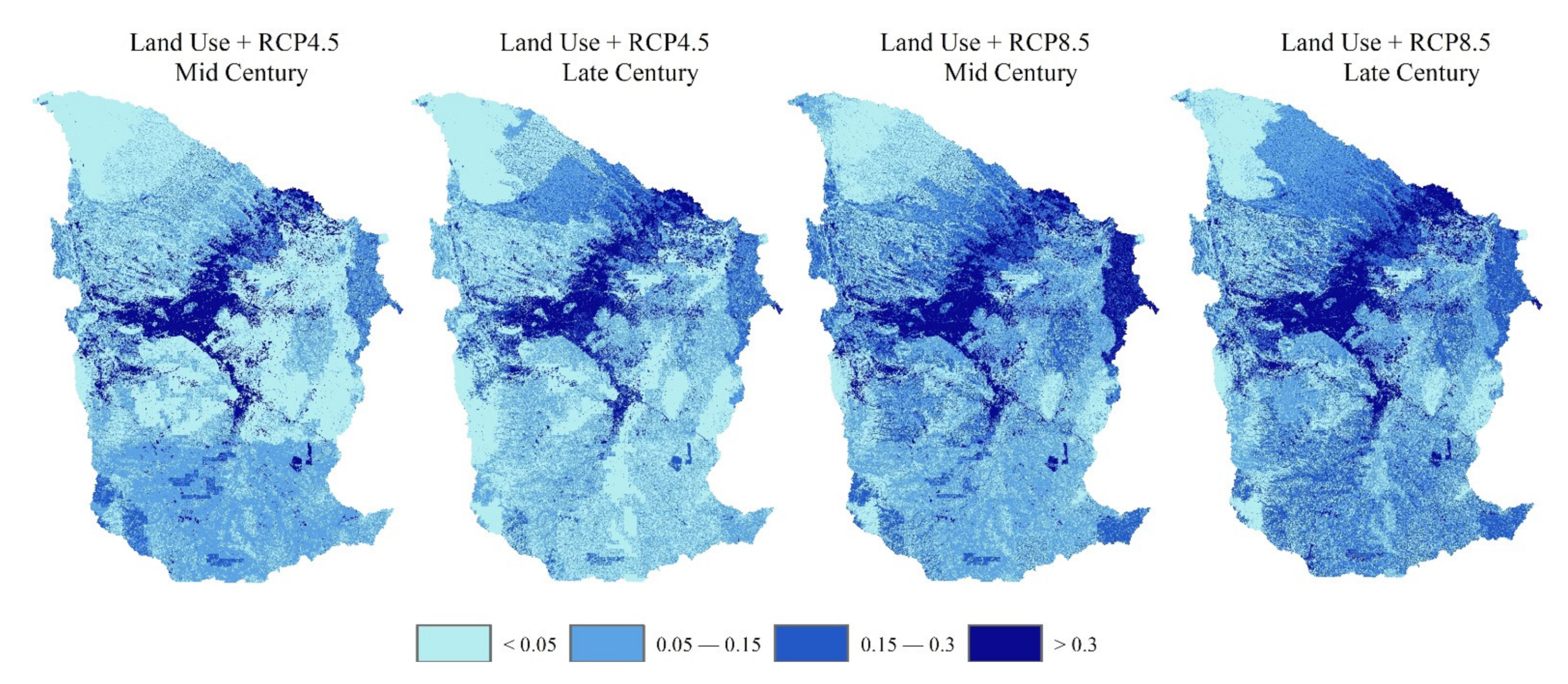
3.4.3. Due to Climate and Land Use

Combining land use and climate change impacts resulted in increased surface runoff generated in both climate scenarios compared to climate change contributions alone. Under the RCP4.5 scenarios, there is an average increase of 21.24 mm (+52.20%) in the surface runoff generated, while RCP8.5 projects a substantial increase in surface runoff depth (+56 mm between 2050 and 2059, and +29.97 mm between 2080 and 2089). Although there is a projected decline in rainfall intensity between 2076 and 2100, the average annual runoff depth increased by 4%. This highlights the resilience of LULC and its dominance in the combined scenarios driven by an increase in urban land use and a decrease in forest and grasslands quotas.

Table 9. Changes in watershed annual surface runoff coefficients $\left(\Delta \propto \right).$

	Land Use	Climate		Climate + Land Use
	Baseline	RCP4.5	RCP8.5	RCP4.5	RCP8.5
1984–1990	-	-	-	-	-
2003–2009	0.0040	-	-	-	-
2010–2016	0.0208	-	-	-	-
2051–2059	-	−0.0185	0.0455	0.0441	0.0838
2081–2089	-	−0.0072	−0.0040	0.0004	0.0069

summarises changes in surface runoff coefficients under all three scenarios. Both land use and climate/land use scenarios exhibit a positive increase in rainfall-runoff ratio while the climate scenario exhibits otherwise.

Combining the effects of LULC and climate change on watershed hydrologic responses can be very complex due to the unique feedbacks of each independent hydrometeorological parameters. While caution must be taken when the model results are interpreted or reported, heuristic measured values provide a basis for quantifying and understanding the feedback’s magnitudes. Although the LULC is expected to catalyse the surface runoff response, climate change has both probabilities (to decrease or increase the surface runoff) based on their measured/projected output. For example, the effects of climate/land use under RCP4.5 are more significant than that of climate alone, suggesting that LULC could be the primary determinant of hydrological response. Under the RCP4.5 climate/land use scenario, the runoff coefficient between 2050 and 2059 increased by an average of 93.99%, while it decreased by 35.35% in the climate only scenario. Overall, decreased precipitation between 2076 and 2100 reduced the average surface runoff coefficient by 0.0072 (−21.24%), while the combined simulation of land use and climate change remained relatively unchanged. (+0.0004, +0.75%). However, the high emission scenario (RCP8.5) simulated almost a double increase in surface runoff coefficient (+0.0838, +178.83%) compared to the average climate condition under RCP4.5 (0.0469). These discrepancies indicate that extreme weather conditions and significant landcover changes (especially grasslands, urban and agricultural land classes) could result in severe hydrometeorological conditions. Increased runoff coefficient is seen mostly in urban and agricultural land classes that dominate the watershed’s upper and middle reaches (Figure 10).

Similar studies in tropical areas are still limited, especially in dynamic urban watersheds. However, the present studies suggest positive variations under land use and climate change scenarios. Lucas-Borja et al. [99] found that maximum runoff coefficients increased by 23.3% on average compared to the baseline scenario in a tropical Brazilian watershed primarily driven by forest land conversion to agricultural use. However, in an Ethiopian highland, the combined climate and LULC scenario were comparable to climate change only due to the observed decrease in surface runoff, groundwater and total water yield driven by a decrease in precipitation and higher surface temperatures [34].

3.5. Implications of Surface Runoff Change on Water Balance and Quality

Renewable water supplies are critical for the sustainability of terrestrial and marine habitats, as well as human use in agriculture, industry, and households. As increased amounts of water vapour are anticipated in a warmer environment, climate change will alter the hydrological cycle and, thus, the regional freshwater supplies. While rainy areas are expected to become wetter and dry regions drier, the NMA watershed has high potential evapotranspiration, resulting in increased water loss through evapotranspiration. Consequential impacts will differ regionally; where rainfall is estimated to be lower in the future, especially in the southern part of the watershed, a decrease in water resources is expected. Increased temperatures and reduced rainfall between 2076 and 2100 would decrease surface and groundwater supplies, increase plant evapotranspiration and increase evaporation rates from open water and water infrastructure. In the western and northern regions where rainfall is estimated to be higher in the future, an increase in water supplies can be expected to support terrestrial and freshwater habitats, agriculture and domestic use, but these benefits may be limited due to higher temperatures. Increases in severe precipitation events are also expected to lead to increased surface runoff, regional flooding and fertiliser removal, as well as a decrease in soil water and groundwater recharge in many areas. Anthropogenic land use change will intensify or moderate climate change effects on water supplies, and informed land management strategies need to be established. The warming climate will intensify current pressures on renewable freshwater supplies especially in the water-stressed south regions of the NMA watershed, and will result in intensified competition for water between human and natural systems.

Any land transition and how it is used can influence the exchange of water, energy, greenhouse gasses, non-greenhouse gasses and aerosols between the soil and the atmosphere. LULC thus changes the condition and dynamics of the atmosphere, which, in turn, can dampen or intensify local climate change. Land-induced changes in humidity and wind may affect neighbouring and often more distant regions. In addition to global warming, deforestation and urbanisation, especially in the upper northern reaches, may contribute to surface warming and increases convection, which then increases the relative terrestrial temperature difference. These changes invariably cause incoming solar radiation to be redistributed, resulting in an urban-rural contrast in surface radiance and air temperature, resulting in higher ambient and surface temperatures in urban areas than in adjacent rural areas (urban heat island effect) and a localised rainfall pattern (urban rainfall effects). Grasslands absorb CO₂ to be used for growth and continuation. Forests also confine more carbon in their wood and soils than cropland, and the conversion of forests and grasslands in the watershed to cropland, for example, may result in CO₂ emissions to the atmosphere, thereby accelerating the global warming caused by greenhouse gasses. Terrestrial habitats are sources and sinks of chemical compounds such as nitrogen and ozone. Although the watershed rainfall formation is complex, biogenic volatile organic compounds (BVOCs) from increasing agricultural land use may contribute to the formation of tropospheric ozone and secondary aerosols that influence both surface and cloud formation [100]. Shrublands further emit dust as also do the cropland areas after harvesting. An increase in these aerosol volumes in the atmosphere influences temperature positively and negatively, depending on the size, altitude, and composition of the particles. While global warming can affect the land’s functioning and condition, it is not a one-way relationship, as changes in land use/land cover will also influence climate change and, thus, modulate climate change. Understanding this two-way relationship will help to improve adaptation and mitigation strategies and manage the NMA watershed ecosystem.

While this research’s findings focus on alternative data sources and quantification of probable effects land use and climate scenarios, landscape vulnerability should be tested based on integrated surface water management such as controlled development, green infrastructure, sustainable urban drainage designs (SUDS), and water-sensitive urban designs (WSUD). These concepts should encompass greening open spaces, idle land use management, climate change adaptation to land use plans, and ecological functions to maintain water balance by providing a natural water cycle system and improving water quality through guided suitability analysis of waste disposal sites.

The realisation of climate/land use implication on hydrological response is still farfetched as scaling climate/land use models to understand hydrological processes are exceedingly complicated. Critical issues lie in predicting precipitation as climate models cannot provide exact scenarios, especially in individual land classes. For example, models do not include the local effects of urban heat intensity and urban rainfall effects. Further, land use is also interconnected through intricate patchworks of the artificial and natural environment and can be estimated on contributing landscape scale, resulting in complex rainfall-runoff transformations.

4. Conclusions

Rainfall runoff models are input-dependent and require that gridded data have the threshold accuracies in representing the corresponding input parameters’ actual observations. The successful calibration of rainfall runoff models depends highly on rainfall observation to capture the observed precipitation patterns and trends. CHIRPS and CHIRTS datasets yielded a high observed-simulated streamflow correlation (≥0.91) and Nash–Sutcliffe efficiency (≥0.89) in all calibration and validation phases, implying that CHIRPS/CHIRTS datasets can provide valuable and dependable alternative data for climate services. While the model accuracies cannot depend only on the inputs, model algorithms play a significant role in estimating physical variables used in the model execution. The ability of SWAT+ to perform functions with high integrity suggests that SWAT+ model algorithms can represent real-world physical environments with remarkable accuracy. Further, sensitivity analysis, model calibration, and validation procedures are essential in optimising parameters, determining input/output errors and detecting/quantifying model biases. SWAT+ model can be calibrated successfully using IPEAT+.

Climate and land use utilisation are vital parameters in hydrological response, especially in surface runoff generation. In particular, land use has a significant influence on surface runoff change compared to climate changes. Land use plays an essential role in determining the amount of percolating water, surface runoff, and the lost water to the atmosphere through evapotranspiration. The principal drivers of surface runoff generation in the NMA watershed are a rise in the urban area and agricultural land and a loss of grasslands. The effects of climate change cannot be neglected since their combined effects are exponential. The explicit nature of the results of the study requires critical adaptation of sustainable land practises tailored to counter the inevitable pressures of demand for land use, particularly in these rapidly urbanising ecosystems. While such findings can only provide scenarios, patterns, and insights into these changes, cities’ scientific planning is essential in controlling extreme rainfall-related events by considering these scenarios. These data and models’ availability provides essential prerequisites to develop, evaluate and compare different sustainable practices against these findings.

The realisation of climate/land use implication on hydrological response is still farfetched as scaling climate/land use models to understand hydrological processes are exceedingly complicated. Critical issues lie in predicting precipitation as climate models cannot provide exact scenarios or local feedback factors. For example, models do not include the local effects of urban heat intensity and urban rainfall effects. Land use is also interconnected through intricate patchworks of the artificial and natural environment and can be estimated on contributing landscape scale, resulting in complex rainfall runoff transformations which the models oversimplify. Future models should consider land use as complex entities with their local feedback and not generalised only by roughness coefficients and curve numbers.

The study fundamentally highlights the reliability of gridded data as an alternative to instrumental measurements in limited or missing data cases. Further, it highlights the SWAT+ model’s integrity in hydrological simulations and underscores climate/land use change impacts on local hydrology. This research provides a basis for land-use planners on strategies, adaptations and empirical analysis of sustainable development practices for a balanced ecological urban watershed.

References

1. Dale, V.H.; Efroymson, R.A.; Kline, K.L. The land use-climate change-energy nexus. Landsc. Ecol. 2011. [Google Scholar] [CrossRef]
2. Smith, B.D.; Zeder, M.A. The onset of the Anthropocene. Anthropocene 2013. [Google Scholar] [CrossRef]
3. Crutzen, P.J. The Anthropocene. In Earth System Science in the Anthropocene; Springer: Berlin/Heidelberg, Germany, 2006; ISBN 3540265880. [Google Scholar]
4. Lewis, S.L.; Maslin, M.A. Defining the Anthropocene. Nature 2015, 519, 171–180. [Google Scholar] [CrossRef]
5. Zalasiewicz, J.; Williams, M.; Haywood, A.; Ellis, M. The anthropocene: A new epoch of geological time? Philos. Trans. R. Soc. A Math. Phys. Eng. Sci. 2011, 369, 835–841. [Google Scholar] [CrossRef] [Green Version]
6. Ellis, E.C.; Goldewijk, K.K.; Siebert, S.; Lightman, D.; Ramankutty, N. Anthropogenic transformation of the biomes, 1700 to 2000. Glob. Ecol. Biogeogr. 2010, 19, 589–606. [Google Scholar] [CrossRef]
7. Ellis, E.C.; Beusen, A.H.W.; Goldewijk, K.K. Anthropogenic biomes: 10,000 BCE to 2015 CE. Land 2020, 9, 129. [Google Scholar] [CrossRef]
8. Fu, B.J.; Wang, Y.F.; Lu, Y.H.; He, C.S.; Chen, L.D.; Song, C.J. The effects of land-use combinations on soil erosion: A case study in the Loess Plateau of China. Prog. Phys. Geogr. 2009, 33, 793–804. [Google Scholar] [CrossRef]
9. Lin, Y.P.; Hong, N.M.; Wu, P.J.; Wu, C.F.; Verburg, P.H. Impacts of land use change scenarios on hydrology and land use patterns in the Wu-Tu watershed in Northern Taiwan. Landsc. Urban Plan. 2007, 80, 111–126. [Google Scholar] [CrossRef]
10. Pielke, R.A.; Avissar, R. Influence of landscape structure on local and regional climate. Landsc. Ecol. 1990, 4, 133–155. [Google Scholar] [CrossRef]
11. Yeh, C.T.; Huang, S.L. Investigating spatiotemporal patterns of landscape diversity in response to urbanization. Landsc. Urban Plan. 2009, 93, 151–162. [Google Scholar] [CrossRef]
12. Randhir, T.O.; Tsvetkova, O. Spatiotemporal dynamics of landscape pattern and hydrologic process in watershed systems. J. Hydrol. 2011, 404, 1–12. [Google Scholar] [CrossRef]
13. Mohammady, M.; Moradi, H.R.; Zeinivand, H.; Temme, A.J.A.M.; Yazdani, M.R.; Pourghasemi, H.R. Modeling and assessing the effects of land use changes on runoff generation with the CLUE-s and WetSpa models. Theor. Appl. Climatol. 2018, 133, 459–471. [Google Scholar] [CrossRef]
14. Huong, H.T.L.; Pathirana, A. Urbanization and climate change impacts on future urban flooding in Can Tho city, Vietnam. Hydrol. Earth Syst. Sci. 2013, 17, 379–394. [Google Scholar] [CrossRef] [Green Version]
15. Brath, A.; Montanari, A.; Moretti, G. Assessing the effect on flood frequency of land use change via hydrological simulation (with uncertainty). J. Hydrol. 2006, 324, 141–153. [Google Scholar] [CrossRef]
16. IPCC. IPCC Fourth Assessment Report, Climate Change 2007: Impacts, Adaptation and Vulnerability; Working Group II Contribution to the 4th Assessment Report; IPCC: Geneva, Switzerland, 2007; ISBN 0521705975. [Google Scholar]
17. IPCC. IPCC—Fifth Assessment Report (AR5) WGII; IPCC: Geneva, Switzerland, 2014. [Google Scholar]
18. Metz, B.; Meyer, L.; Bosch, P. Climate Change 2007: Mitigation of Climate Change; IPCC: Geneva, Switzerland, 2007; ISBN 9780511546013. [Google Scholar]
19. Steele-Dunne, S.; Lynch, P.; McGrath, R.; Semmler, T.; Wang, S.; Hanafin, J.; Nolan, P. The impacts of climate change on hydrology in Ireland. J. Hydrol. 2008, 356, 28–45. [Google Scholar] [CrossRef]
20. Boyer, C.; Chaumont, D.; Chartier, I.; Roy, A.G. Impact of climate change on the hydrology of St. Lawrence tributaries. J. Hydrol. 2010, 384, 65–83. [Google Scholar] [CrossRef]
21. Yang, N.; Men, B.H.; Lin, C.K. Impact analysis of climate change on water resources. Procedia Eng. 2011, 24, 643–648. [Google Scholar]
22. IPCC. Climate Change and Land: An IPCC Special Report on Climate Change, Desertification, Land Degradation, Sustainable Land Management, Food Security, and Greenhouse Gas Fluxes in Terrestrial Ecosystems; IPCC: Geneva, Switzerland, 2019. [Google Scholar]
23. Vaze, J.; Post, D.A.; Chiew, F.H.S.; Perraud, J.M.; Viney, N.R.; Teng, J. Climate non-stationarity—Validity of calibrated rainfall-runoff models for use in climate change studies. J. Hydrol. 2010, 394, 447–457. [Google Scholar] [CrossRef]
24. Araos, M.; Berrang-Ford, L.; Ford, J.D.; Austin, S.E.; Biesbroek, R.; Lesnikowski, A. Climate change adaptation planning in large cities: A systematic global assessment. Environ. Sci. Policy 2016, 66, 375–382. [Google Scholar] [CrossRef]
25. Winsemius, H.C.; Aerts, J.C.J.H.; Van Beek, L.P.H.; Bierkens, M.F.P.; Bouwman, A.; Jongman, B.; Kwadijk, J.C.J.; Ligtvoet, W.; Lucas, P.L.; Van Vuuren, D.P.; et al. Global drivers of future river flood risk. Nat. Clim. Chang. 2016, 6, 381–385. [Google Scholar] [CrossRef]
26. Mozumder, P.; Flugman, E.; Randhir, T. Adaptation behavior in the face of global climate change: Survey responses from experts and decision makers serving the Florida Keys. Ocean Coast. Manag. 2011, 54, 37–44. [Google Scholar] [CrossRef]
27. Quevauviller, P. Adapting to climate change: Reducing water-related risks in Europe—EU policy and research considerations. Environ. Sci. Policy 2011, 14, 722–729. [Google Scholar] [CrossRef]
28. Forsee, W.J.; Ahmad, S. Evaluating Urban Storm-Water Infrastructure Design in Response to Projected Climate Change. J. Hydrol. Eng. 2011, 16, 865–873. [Google Scholar] [CrossRef]
29. Bormann, H.; Breuer, L.; Gräff, T.; Huisman, J.A.; Croke, B. Assessing the impact of land use change on hydrology by ensemble modelling (LUCHEM) IV: Model sensitivity to data aggregation and spatial (re-)distribution. Adv. Water Resour. 2009, 32, 171–192. [Google Scholar] [CrossRef]
30. Tang, L.; Yang, D.; Hu, H.; Gao, B. Detecting the effect of land-use change on streamflow, sediment and nutrient losses by distributed hydrological simulation. J. Hydrol. 2011, 409, 172–182. [Google Scholar] [CrossRef]
31. Li, Z.; Liu, W.Z.; Zhang, X.C.; Zheng, F.L. Impacts of land use change and climate variability on hydrology in an agricultural catchment on the Loess Plateau of China. J. Hydrol. 2009, 377, 35–42. [Google Scholar] [CrossRef]
32. Pervez, M.S.; Henebry, G.M. Assessing the impacts of climate and land use and land cover change on the freshwater availability in the Brahmaputra River basin. J. Hydrol. Reg. Stud. 2015, 3, 285–311. [Google Scholar] [CrossRef] [Green Version]
33. Karlsson, I.B.; Sonnenborg, T.O.; Refsgaard, J.C.; Trolle, D.; Børgesen, C.D.; Olesen, J.E.; Jeppesen, E.; Jensen, K.H. Combined effects of climate models, hydrological model structures and land use scenarios on hydrological impacts of climate change. J. Hydrol. 2016, 535, 301–317. [Google Scholar] [CrossRef]
34. Dibaba, W.T.; Demissie, T.A.; Miegel, K. Watershed hydrological response to combined land use/land cover and climate change in highland ethiopia: Finchaa catchment. Water 2020, 12, 1801. [Google Scholar] [CrossRef]
35. Githui, F.; Mutua, F.; Bauwens, W. Estimating the impacts of land-cover change on runoff using the soil and water assessment tool (SWAT): Case study of Nzoia catchment, Kenya/Estimation des impacts du changement d’occupation du sol sur l’écoulement à l’aide de SWAT: Étude du cas du bassi. Hydrol. Sci. J. 2009, 54, 899–908. [Google Scholar] [CrossRef]
36. Musau, J.; Sang, J.; Gathenya, J.; Luedeling, E. Hydrological responses to climate change in Mt. Elgon watersheds. J. Hydrol. Reg. Stud. 2015. [Google Scholar] [CrossRef] [Green Version]
37. Mango, L.M.; Melesse, A.M.; McClain, M.E.; Gann, D.; Setegn, S.G. Land use and climate change impacts on the hydrology of the upper Mara River Basin, Kenya: Results of a modeling study to support better resource management. Hydrol. Earth Syst. Sci. 2011, 15, 2245–2258. [Google Scholar] [CrossRef] [Green Version]
38. Seiller, G.; Anctil, F.; Perrin, C. Multimodel evaluation of twenty lumped hydrological models under contrasted climate conditions. Hydrol. Earth Syst. Sci. 2012, 16, 1171–1189. [Google Scholar] [CrossRef] [Green Version]
39. Roy, T.; Gupta, H.V.; Serrat-Capdevila, A.; Valdes, J.B. Using satellite-based evapotranspiration estimates to improve the structure of a simple conceptual rainfall-runoff model. Hydrol. Earth Syst. Sci. 2017, 21, 879–896. [Google Scholar] [CrossRef] [Green Version]
40. Rozos, E. A methodology for simple and fast streamflow modelling. Hydrol. Sci. J. 2020, 65, 1084–1095. [Google Scholar] [CrossRef]
41. Zhang, H.; Huang, G.H.; Wang, D.; Zhang, X. Multi-period calibration of a semi-distributed hydrological model based on hydroclimatic clustering. Adv. Water Resour. 2011. [Google Scholar] [CrossRef]
42. Kim, N.W.; Chung, I.M.; Won, Y.S.; Arnold, J.G. Development and application of the integrated SWAT-MODFLOW model. J. Hydrol. 2008, 356, 1–16. [Google Scholar] [CrossRef]
43. Arnold, J.G.; Moriasi, D.N.; Gassman, P.W.; Abbaspour, K.C.; White, M.J.; Srinivasan, R.; Santhi, C.; Harmel, R.D.; Van Griensven, A.; Van Liew, M.W.; et al. SWAT: Model use, calibration, and validation. Trans. ASABE 2012, 55, 1491–1508. [Google Scholar] [CrossRef]
44. Abbott, M. Distributed Hydrological Modelling; Kluwer Academic: Dordrecht, The Netherlands; Boston, MA, USA, 1996; ISBN 0792340426. [Google Scholar]
45. Beven, K.; Binley, A. The future of distributed models: Model calibration and uncertainty prediction. Hydrol. Process. 1992. [Google Scholar] [CrossRef]
46. Immerzeel, W.W.; Droogers, P. Calibration of a distributed hydrological model based on satellite evapotranspiration. J. Hydrol. 2008, 349, 411–424. [Google Scholar] [CrossRef]
47. Francesconi, W.; Srinivasan, R.; Pérez-Miñana, E.; Willcock, S.P.; Quintero, M. Using the Soil and Water Assessment Tool (SWAT) to model ecosystem services: A systematic review. J. Hydrol. 2016, 535, 625–636. [Google Scholar] [CrossRef]
48. Jayakrishnan, R.; Srinivasan, R.; Santhi, C.; Arnold, J.G. Advances in the application of the SWAT model for water resources management. Hydrol. Process. 2005, 19, 749–762. [Google Scholar] [CrossRef]
49. Radcliffe, D.E.; Reid, D.K.; Blombäck, K.; Bolster, C.H.; Collick, A.S.; Easton, Z.M.; Francesconi, W.; Fuka, D.R.; Johnsson, H.; King, K.; et al. Applicability of Models to Predict Phosphorus Losses in Drained Fields: A Review. J. Environ. Qual. 2015, 44, 614–628. [Google Scholar] [CrossRef]
50. Krysanova, V.; White, M. Advances in water resources assessment with SWAT—An overview. Hydrol. Sci. J. 2015. [Google Scholar] [CrossRef] [Green Version]
51. Glavan, M.; Pintar, M.; Urbanc, J. Spatial variation of crop rotations and their impacts on provisioning ecosystem services on the river Drava alluvial plain. Sustain. Water Qual. Ecol. 2015, 5, 31–48. [Google Scholar] [CrossRef]
52. Arnold, J.G.; Kiniry, J.R.; Srinivasan, R.; Williams, J.R.; Haney, E.B.; Neitsch, S.L. Soil and Water Assessment Tool; Input/Output Documentation, TR-439; Texas Water Resources Institute: Huston, TX, USA, 2012. [Google Scholar]
53. Dile, Y.T.; Daggupati, P.; George, C.; Srinivasan, R.; Arnold, J. Introducing a new open source GIS user interface for the SWAT model. Environ. Model. Softw. 2016, 85, 129–138. [Google Scholar] [CrossRef]
54. Molina-Navarro, E.; Nielsen, A.; Trolle, D. A QGIS plugin to tailor SWAT watershed delineations to lake and reservoir waterbodies. Environ. Model. Softw. 2018, 108, 67–71. [Google Scholar] [CrossRef]
55. Reddy, N.N.; Reddy, K.V.; Vani, J.S.L.S.; Daggupati, P.; Srinivasan, R. Climate change impact analysis on watershed using QSWAT. Spat. Inf. Res. 2018, 26, 253–259. [Google Scholar] [CrossRef]
56. Tanksali, A.; Soraganvi, V.S. Assessment of impacts of land use/land cover changes upstream of a dam in a semi-arid watershed using QSWAT. Model. Earth Syst. Environ. 2020. [Google Scholar] [CrossRef]
57. Bansode, S.; Patil, K. Water Balance Assessment using Q-SWAT Rheological Properties of Nanoclay Modified Bitumen View project Water Balance Assessment using Q-SWAT. Artic. Int. J. Eng. Res. 2016, 5, 515–518. [Google Scholar]
58. Munoth, P.; Goyal, R. Effects of area threshold values and stream burn-in process on runoff and sediment yield using QSWAT model. ISH J. Hydraul. Eng. 2019. [Google Scholar] [CrossRef]
59. Ledesma, J.L.J.; Futter, M.N. Gridded climate data products are an alternative to instrumental measurements as inputs to rainfall–runoff models. Hydrol. Process. 2017, 31, 3283–3293. [Google Scholar] [CrossRef] [Green Version]
60. Afrifa-Yamoah, E.; Mueller, U.A.; Taylor, S.M.; Fisher, A.J. Missing data imputation of high-resolution temporal climate time series data. Meteorol. Appl. 2020. [Google Scholar] [CrossRef]
61. Vu, M.T.; Raghavan, S.V.; Liong, S.Y. SWAT use of gridded observations for simulating runoff—A Vietnam river basin study. Hydrol. Earth Syst. Sci. 2012, 16, 2801–2811. [Google Scholar] [CrossRef] [Green Version]
62. Try, S.; Tanaka, S.; Tanaka, K.; Sayama, T.; Oeurng, C.; Uk, S.; Takara, K.; Hu, M.; Han, D. Comparison of gridded precipitation datasets for rainfall-runoff and inundation modeling in the Mekong River Basin. PLoS ONE 2020. [Google Scholar] [CrossRef] [Green Version]
63. Funk, C.; Peterson, P.; Landsfeld, M.; Pedreros, D.; Verdin, J.; Shukla, S.; Husak, G.; Rowland, J.; Harrison, L.; Hoell, A.; et al. The climate hazards infrared precipitation with stations—A new environmental record for monitoring extremes. Sci. Data 2015. [Google Scholar] [CrossRef] [PubMed] [Green Version]
64. Funk, C.; Peterson, P.; Peterson, S.; Shukla, S.; Davenport, F.; Michaelsen, J.; Knapp, K.R.; Landsfeld, M.; Husak, G.; Harrison, L.; et al. A high-resolution 1983–2016 TMAX climate data record based on infrared temperatures and stations by the climate hazard center. J. Clim. 2019, 32, 5639–5658. [Google Scholar] [CrossRef]
65. Qin, L.; He, Y.; Huang, W.; Ma, G. Analysis of the rainfall and runoff temporal variation of Jialing River during 1955–2006. In Proceedings of the 11th Asian Conference on Chemical Sensors (ACCS2015), Penang, Malaysia, 16–18 November 2015; Volume 1820, p. 80008. [Google Scholar] [CrossRef]
66. Liu, X.; Liang, X.; Li, X.; Xu, X.; Ou, J.; Chen, Y.; Li, S.; Wang, S.; Pei, F. A future land use simulation model (FLUS) for simulating multiple land use scenarios by coupling human and natural effects. Landsc. Urban Plan. 2017, 168, 94–116. [Google Scholar] [CrossRef]
67. Luo, M.; Li, X. Forest Loss Simulation and Water Yield Assessment Based on GEOSOS-FLUS Model: A Case Study of Yangtze River Delta and Pearl River Delta. In Proceedings of the International Geoscience and Remote Sensing Symposium (IGARSS), Madrid, Spain, 13–16 September 2019; pp. 6582–6585. [Google Scholar]
68. Li, X.; Chen, G.; Liu, X.; Liang, X.; Wang, S.; Chen, Y.; Pei, F.; Xu, X. A New Global Land-Use and Land-Cover Change Product at a 1-km Resolution for 2010 to 2100 Based on Human-Environment Interactions. Ann. Am. Assoc. Geogr. 2017, 107, 1040–1059. [Google Scholar] [CrossRef]
69. Wang, Y.; Shen, J.; Yan, W.; Chen, C. Backcasting approach with multi-scenario simulation for assessing effects of land use policy using GeoSOS-FLUS software. MethodsX 2019, 6, 1384–1397. [Google Scholar] [CrossRef] [PubMed]
70. Kim, J.; Waliser, D.E.; Mattmann, C.A.; Goodale, C.E.; Hart, A.F.; Zimdars, P.A.; Crichton, D.J.; Jones, C.; Nikulin, G.; Hewitson, B.; et al. Evaluation of the CORDEX-Africa multi-RCM hindcast: Systematic model errors. Clim. Dyn. 2014, 42, 1189–1202. [Google Scholar] [CrossRef]
71. Van Vuuren, D.P.; Edmonds, J.; Kainuma, M.; Riahi, K.; Thomson, A.; Hibbard, K.; Hurtt, G.C.; Kram, T.; Krey, V.; Lamarque, J.F.; et al. The representative concentration pathways: An overview. Clim. Chang. 2011, 109, 5–31. [Google Scholar] [CrossRef]
72. Riahi, K.; Grübler, A.; Nakicenovic, N. Scenarios of long-term socio-economic and environmental development under climate stabilization. Technol. Forecast. Soc. Chang. 2007, 74, 887–935. [Google Scholar] [CrossRef]
73. Gadissa, T.; Nyadawa, M.; Behulu, F.; Mutua, B. The effect of climate change on loss of lake volume: Case of sedimentation in Central Rift Valley Basin, Ethiopia. Hydrology 2018, 5, 67. [Google Scholar] [CrossRef] [Green Version]
74. Rathjens, H.; Bieger, K.; Srinivasan, R.; Arnold, J.G. CMhyd User Manual Documentation for Preparing Simulated Climate Change Data for Hydrologic Impact Studies; SWAT: Huston, TX, USA, 2016. [Google Scholar]
75. Fang, G.H.; Yang, J.; Chen, Y.N.; Zammit, C. Comparing bias correction methods in downscaling meteorological variables for a hydrologic impact study in an arid area in China. Hydrol. Earth Syst. Sci. 2015, 19, 2547–2559. [Google Scholar] [CrossRef] [Green Version]
76. Zhang, B.; Shrestha, N.K.; Daggupati, P.; Rudra, R.; Shukla, R.; Kaur, B.; Hou, J. Quantifying the impacts of climate change on streamflow dynamics of two major rivers of the Northern Lake Erie basin in Canada. Sustainability 2018, 10, 2897. [Google Scholar] [CrossRef] [Green Version]
77. Setegn, S.G.; Srinivasan, R.; Dargahi, B. Hydrological Modelling in the Lake Tana Basin, Ethiopia Using SWAT Model. Open Hydrol. J. 2008, 2, 49–62. [Google Scholar] [CrossRef] [Green Version]
78. Soil Conservation Service Engineering Division. Section 4: Hydrology. In National Engineering Handbook; NRCS: Washington, DC, USA, 1972. [Google Scholar]
79. Yen, H.; Park, S.; Arnold, J.G.; Srinivasan, R.; Chawanda, C.J.; Wang, R.; Feng, Q.; Wu, J.; Miao, C.; Bieger, K.; et al. IPEAT+: A built-in optimization and automatic calibration tool of SWAT. Water 2019, 11, 1681. [Google Scholar] [CrossRef] [Green Version]
80. Haan, C.T. Statistical methods in hydrology. Stat. Methods Hydrol. 1977. [Google Scholar] [CrossRef]
81. Lenhart, T.; Eckhardt, K.; Fohrer, N.; Frede, H.G. Comparison of two different approaches of sensitivity analysis. Phys. Chem. Earth 2002, 27, 645–654. [Google Scholar] [CrossRef]
82. Feyereisen, G.W.; Strickland, T.C.; Bosch, D.D.; Sullivan, D.G. Evaluation of SWAT Manual Calibration and Input Parameter Sensitivity in the Little River Watershed. Trans. ASABE 2007, 50, 843–855. [Google Scholar] [CrossRef]
83. Brouziyne, Y.; Abouabdillah, A.; Bouabid, R.; Benaabidate, L.; Oueslati, O. SWAT manual calibration and parameters sensitivity analysis in a semi-arid watershed in North-western Morocco. Arab. J. Geosci. 2017, 10. [Google Scholar] [CrossRef]
84. Zambrano, M.B. Package “hydroGOF”: Goodness-of-Fit Functions for Comparison of Simulated and Observed Hydrological Time Series; SWAT: Huston, TX, USA, 2017. [Google Scholar]
85. Yapo, P.O.; Gupta, H.V.; Sorooshian, S. Automatic calibration of conceptual rainfall-runoff models: Sensitivity to calibration data. J. Hydrol. 1996. [Google Scholar] [CrossRef]
86. Nash, J.E.; Sutcliffe, J.V. River flow forecasting through conceptual models part I—A discussion of principles. J. Hydrol. 1970, 10, 282–290. [Google Scholar] [CrossRef]
87. Krause, P.; Boyle, D.P.; Bäse, F. Comparison of different efficiency criteria for hydrological model assessment. Adv. Geosci. 2005, 5, 89–97. [Google Scholar] [CrossRef] [Green Version]
88. Gupta, H.V.; Kling, H.; Yilmaz, K.K.; Martinez, G.F. Decomposition of the mean squared error and NSE performance criteria: Implications for improving hydrological modelling. J. Hydrol. 2009. [Google Scholar] [CrossRef] [Green Version]
89. Criss, R.E.; Winston, W.E. Do Nash values have value? Discussion and alternate proposals. Hydrol. Process. 2008, 22, 2723–2725. [Google Scholar] [CrossRef]
90. Hu, S.; Fan, Y.; Zhang, T. Assessing the Effect of Land Use Change on Surface Runoff in a Rapidly Urbanized City: A Case Study of the Central Area of Beijing. Land 2020, 9, 17. [Google Scholar] [CrossRef] [Green Version]
91. Chen, Y.; Li, X.; Liu, X.; Ai, B. Modeling urban land-use dynamics in a fast developing city using the modified logistic cellular automaton with a patch-based simulation strategy. Int. J. Geogr. Inf. Sci. 2014, 28, 234–255. [Google Scholar] [CrossRef]
92. Pontius, R.G.; Boersma, W.; Castella, J.-C.; Clarke, K.; de Nijs, T.; Dietzel, C.; Duan, Z.; Fotsing, E.; Goldstein, N.; Kok, K.; et al. Comparing the input, output, and validation maps for several models of land change. Ann. Reg. Sci. 2008, 42, 11–37. [Google Scholar] [CrossRef] [Green Version]
93. Lyon, B.; Vigaud, N. Unraveling East Africa’s Climate Paradox. Clim. Extrem. Patterns Mech. Geophys. Monogr. 2017, 265, 281. [Google Scholar] [CrossRef]
94. Williams, A.P.; Funk, C. A westward extension of the warm pool leads to a westward extension of the Walker circulation, drying eastern Africa. Clim. Dyn. 2011, 37, 2417–2435. [Google Scholar] [CrossRef] [Green Version]
95. Lyon, B.; Dewitt, D.G. A recent and abrupt decline in the East African long rains. Geophys. Res. Lett. 2012, 39, 1–5. [Google Scholar] [CrossRef] [Green Version]
96. Yang, W.; Seager, R.; Cane, M.A.; Lyon, B. The East African long rains in observations and models. J. Clim. 2014, 27, 7185–7202. [Google Scholar] [CrossRef]
97. Beyene, T.; Lettenmaier, D.P.; Kabat, P. Hydrologic impacts of climate change on the Nile River Basin: Implications of the 2007 IPCC scenarios. Clim. Chang. 2010. [Google Scholar] [CrossRef]
98. Guzha, A.C.; Rufino, M.C.; Okoth, S.; Jacobs, S.; Nóbrega, R.L.B. Impacts of land use and land cover change on surface runoff, discharge and low flows: Evidence from East Africa. J. Hydrol. Reg. Stud. 2018, 15, 49–67. [Google Scholar] [CrossRef]
99. Lucas-Borja, M.E.; Carrà, B.G.; Nunes, J.P.; Bernard-Jannin, L.; Zema, D.A.; Zimbone, S.M. Impacts of land-use and climate changes on surface runoff in a tropical forest watershed (Brazil). Hydrol. Sci. J. 2020, 65, 1–18. [Google Scholar] [CrossRef]
100. Laothawornkitkul, J.; Taylor, J.E.; Paul, N.D.; Hewitt, C.N. Biogenic volatile organic compounds in the Earth system: Tansley review. New Phytol. 2009, 183, 27–51. [Google Scholar] [CrossRef]
101. Nyenzi, B.S.; Kiangi, P.M.R.; Rao, N.N.P. Evaporation values in East Africa. Arch. Meteorol. Geophys. Bioclimatol. Ser. B 1981, 29, 37–55. [Google Scholar] [CrossRef]
102. Karongo, S.K.; Sharma, T.C. An evaluation of actual evapotranspiration in tropical East Africa. Hydrol. Process. 1997, 11, 501–510. [Google Scholar] [CrossRef]
103. Dagg, M.; Woodhead, T.; Rijks, D.A. Evaporation in East Africa. Int. Assoc. Sci. Hydrol. Bull. 1970, 15, 61–67. [Google Scholar] [CrossRef] [Green Version]
104. Alemayehu, T.; van Griensven, A.; Senay, G.B.; Bauwens, W. Evapotranspiration Mapping in a Heterogeneous Landscape Using Remote Sensing and Global Weather Datasets: Application to the Mara Basin, East Africa. Remote Sens. 2017, 9, 390. [Google Scholar] [CrossRef] [Green Version]
Figure 1. Study Area. The Nairobi Metropolitan Area (NMA) covers partly neighbouring Kajiado, Machakos and Kiambu counties.
Hydrology 08 00048 g001
Figure 2. Watershed’s soil composition and elevation distribution. Eutric vertisols are the most dominant soils, while the elevation is high on the western bounds. The watershed was calibrated using gauging station 3DA02.
Hydrology 08 00048 g002
Figure 3. Class-to-class land-use transition changes in square kilometres. Black bars represent unchanged land class area while blue denotes the respective conversion to individual classes.
Hydrology 08 00048 g003
Figure 4. Maps showing land use land cover distribution. The first four maps show historical LULC classified from Landsat imageries, while the latter two represent projected land use distribution.
Hydrology 08 00048 g004
Figure 5. Taylor diagrams: Model skill and biases. The plots display individual model correlation coefficient, standard deviation and% bias compared to CHIRPS and CHIRTS datasets. The red markers and labels represent RCP8.5, while blue markers and labels represent RCP8.5. Note that the shape variation of markers corresponds to the percentage bias sizes.
Hydrology 08 00048 g005
Figure 6. Model precipitation trends at a sample station (a) Annual precipitation trends, (b) March–April–May (MAM) seasonal trend, (c) June–July–August (JJA) seasonal trend, and (d) October–February (ON + DJF) Seasonal trend.
Hydrology 08 00048 g006
Figure 7. Model mean surface temperature trends at a sample station. (a) Annual precipitation trends, (b) March–April–May (MAM) seasonal trend, (c) June–July–August (JJA) seasonal trend, and (d) October–February (ON + DJF) seasonal trend.
Hydrology 08 00048 g007
Figure 8. Calibration results. (a) Calibration phase, (b,c) validation phase and (d) goodness-of-fit coefficients.
Hydrology 08 00048 g008
Figure 9. Historical annual surface runoff depth in millimetres (mm) for the epochs (a) 1984–1990, (b), 2003–2009, (c) 2010–2016.
Hydrology 08 00048 g009
Figure 10. Annual surface runoff coefficient distribution under both climate scenarios.
Hydrology 08 00048 g010