
Modeling Climate Change Impacts on Water Balance of a Mediterranean Watershed Using SWAT+


1
CREA-Research Centre for Agricultural Policies and Bioeconomy, 00198 Rome, Italy
2
Bayer CropScience, 700 Chesterfield Parkway West, Chesterfield, MO 63017, USA
3
College of Environmental Science and Engineering, Tongji University, No 1239, Siping Road, Shanghai 200092, China
*
Author to whom correspondence should be addressed.
Hydrology 2021, 8(4), 157; https://0-doi-org.brum.beds.ac.uk/10.3390/hydrology8040157
Submission received: 24 September 2021
/
Revised: 11 October 2021
/
Accepted: 12 October 2021
/
Published: 15 October 2021
(This article belongs to the Special Issue Sustainable Water Management in Urban, Agricultural and Natural Systems)
Abstract
:The consequences of climate change on food security in arid and semi-arid regions can be serious. Understanding climate change impacts on water balance is critical to assess future crop performance and develop sustainable adaptation strategies. This paper presents a climate change impact study on the water balance components of an agricultural watershed in the Mediterranean region. The restructured version of the Soil and Water Assessment Tool (SWAT+) model was used to simulate the hydrological components in the Sulcis watershed (Sardinia, Italy) for the baseline period and compared to future climate projections at the end of the 21st century. The model was forced using data from two Regional Climate Models under the representative concentration pathways RCP4.5 and RCP8.5 scenarios developed at a high resolution over the European domain. River discharge data were used to calibrate and validate the SWAT+ model for the baseline period, while the future hydrological response was evaluated for the mid-century (2006–2050) and late-century (2051–2098). The model simulations indicated a future increase in temperature, decrease in precipitation, and consequently increase in potential evapotranspiration in both RCP scenarios. Results show that these changes will significantly decrease water yield, surface runoff, groundwater recharge, and baseflow. These results highlight how hydrological components alteration by climate change can benefit from modelling high-resolution future scenarios that are useful for planning mitigation measures in agricultural semi-arid Mediterranean regions.
1. Introduction
Climate and land-use change are significantly impacting water resources and altering the precipitation regime and the components of the hydrological cycle [1]. These alterations are putting rising pressures on freshwater-related ecosystem services and, consequently, on their ability to sustain ecosystems, biodiversity, agriculture production, and human water need [2].
Agriculture is one of the sectors most dependent on climate as it directly impacts crop productivity. More frequent extreme events such as droughts have had adverse effects on farmlands in vulnerable areas around the world [3]. This is especially true for arid and semi-arid environments, where water shortage is a chief issue [4]. Meanwhile, the world population is expected to grow upward to 9.7 billion by 2050 [5]. Increasing demand under unfavorable weather conditions put huge pressure on agricultural systems. These circumstances call for the proactive development of sustainable adaptation strategies, which require an understanding of crop performance under projected climate change scenarios. As water availability is a major determinant of crop yield, modeling climate change impacts on water balance is a prerequisite for reliable prediction of future agricultural productivity [6].
The Mediterranean area is particularly exposed to the effects of climate change and consequent alterations in the hydrological regime [7,8]. It was projected that future winters will become wetter and summers drier [9], exacerbating the magnitude and frequency of the extreme weather events experienced in the last decades [10,11].
In recent years, the use of General Circulation Models (GCMs) and Regional Climate Models (RCMs) allows performing reliable and accurate future projections for a range of climate variables at high resolution in time and space. For instance, Leta and Bauwens [12] assessed the impact of future climate change on the hydrological extremes in a river basin in Belgium using statistically downscaled time series data. Similarly, Brouziyne et al. [13] modeled flow regime alterations under projected climate change in a Mediterranean basin forcing the eco-hydrological SWAT model with data from one climate model under two emission scenarios. In the same vein, Vezzoli et al. [14] investigated river discharge in the Po River basin using the TOPKAPI model and regional climate model projections under two different representative concentration pathways (RCPs) [15]. In another study, Fonseca and Santos [16] assessed projected climate change impacts on hydrologic flows applying the HSPF model and a climatic dataset by an ensemble of five different GCM-RCM model chains under two greenhouse gas emission scenarios.
All the above studies suggest a rising interest in modeling accurately internal watershed processes and in simulating reliable scenarios under future climate conditions. In this sense, the Soil and Water Assessment Tool (SWAT) is one of the widely used hydrological models that simulate the watershed processes, water quality, pesticide fate and transport, and the nutrient cycles under various climates and conditions [17,18,19].
SWAT+ is the restructured version of the SWAT model [20,21], allowing a more realistic simulation of river basins and water cycle compared to the previous version [18]. Although extensive research has been conducted using SWAT for modeling the effects of climate change on hydrology [22], to date, few studies have investigated the use of SWAT+ for representing hydrological consequences of climate change. In this study, we test the ability of SWAT+ to model current and future effects of climate change on water balance in a catchment in the Sulcis area (Italy). The specific objectives of this study were: (i) to calibrate and validate the model to adequately represent the hydrological cycle in the current scenario; (ii) to assess the projected changes in terms of climate patterns and water balance under different RCP scenarios; (iii) to discuss potential consequences of these changes in terms of suitable adaptation strategies. To the best of the authors’ knowledge, there is no such study in the Mediterranean region that has assessed the impacts of climate change on water balance on agricultural watersheds using the SWAT+ and RCMs at a higher resolution.
2. Materials and Methods
2.1. Study Area
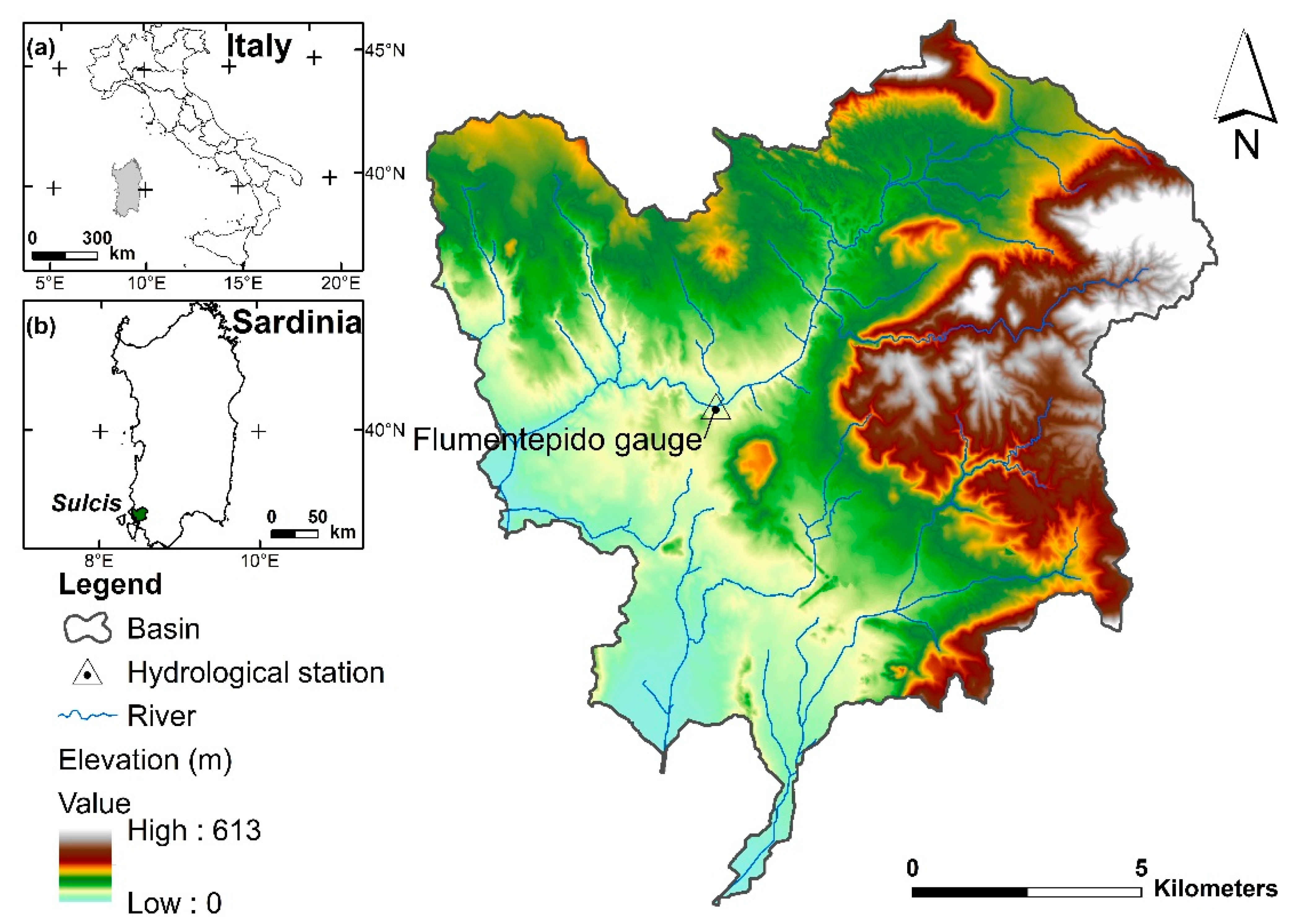
The study area is the Sulcis district in the southwest part of Sardinia Region (Italy), with a total drainage surface of around 173 km2 and an elevation ranging from 1 to 613 m above the mean sea level (39°10’ N, 8°30’ E, Figure 1). The regional climate is classified as Mediterranean semi-arid with a bimodal pattern of precipitation distribution, with a mean annual temperature and rainfall of 16 °C and 648 mm, respectively. The basin is relatively flat, with undulating terrain in the northern part. Agricultural arable land, shrubs and scattered grasses and pasture are the main land cover categories. There is one urban center and few small villages located within the catchment territory.
2.2. Experimental Setup
2.2.1. SWAT+ Model
SWAT is a semi-distributed eco-hydrological model used to simulate the hydrological cycle and sediment transport at the watershed scale. The SWAT model delineated a watershed and sub-watersheds into Hydrologic Response Units (HRUs) that are homogenous spatial units with a unique combination of land use, soil, and slope. Soil water balance is determined within the HRUs. The model was extensively used worldwide in the past at different scales for ecohydrological modeling during different climate conditions and with future climate projections [23,24,25,26].
In this study, the SWAT+ is used. The SWAT+ is a restructured version of SWAT that is more flexible in terms of watershed discretization, configuration, and spatial representation of processes, as well as in defining management schedules and operations, and database maintaining. Advantages include improved anthropogenic water use and management, flexibility in management schedules and operations, easier printing of outputs, and rapid model calibration. Finally, SWAT+ has a free-file format that can be easily managed into a spreadsheet. See Bieger et al. [21] for more details and further explanations on new functions, improvements, and advantages.
SWAT+ models the hydrologic cycle using the water balance equation (Equation (1)):
where SWt i is the final soil water content (mm) on day i, SW0 i is the initial soil water content on day i (mm), t is the time (days), Rday i is the amount of precipitation on day i (mm), Qsurf i is the amount of surface runoff on day i (mm), Ea i is the amount of evapotranspiration on day i (mm), Wseep i is the amount of water entering the vadose zone from the soil profile on day i (mm), and Qgw i is the amount of return flow on day i (mm) [23].
The work has been organized in the following way. First, baseline model simulation is conducted through a four-step procedure (see Figure 2): (i) delineation of the watershed; (ii) creation of the HRU; (iii) editing of inputs and run of the model; (iv) visualization of the results. Second, the model is calibrated and validated using discharge data measured in the field from one gauge station (Figure 1). Finally, climate change projections are computed forcing the validated SWAT+ model by data (daily minimum and maximum temperatures and precipitation) from two RCM under RCP4.5 and RCP8.5 scenarios. In this study, the watershed was delineated using the SWAT+ plugin within QGIS 3.16 [27].
2.2.2. Dataset
The geospatial data required by the SWAT+ model include (Table 1): Digital Elevation Model (DEM), land use/cover data, soil data, and river network. The DEM was used to generate stream networks, the catchment and sub-basin delineation. Land use/cover, soil data and elevations were jointly used to delineate HRUs. The dataset is available from the web-portal of the Autonomous Region of Sardinia (RAS) [28]. The original spatial data were converted and ingested in a grid format at a 10-meter resolution.
Step 1 uses the 10-meter DEM and stream network to derive the watershed, landscape units and sub-basins. In Step 2, we used a land use map (scale 1:25,000) and a soil map (scale 1:50,000) with 21 and 32 map units, respectively. These data provide specific soil properties (e.g., sand, silt, and clay contents, the available water capacity of soil layers) and crop types required for the creation of the HRUs. The dataset provided by RAS is validated in terms of consistency, accuracy, and reliability.
In Step 3, climate data for the period 1979–2005 were used to set up the baseline scenario covering a reasonable time span before future periods simulations. Climate variables include daily maximum and minimum temperature, precipitation, solar radiation, relative humidity, and wind speed obtained from the Climate Forecast System Reanalysis [29]. In this step, prior to the simulation starts, the warm-up period of three years was set along with other attributes such as the curve number (a function of the soil moisture) and the water routing as a variable storage method.

Table 1.
Dataset used for modeling water balance under the baseline period.
| Data | Resolution | Date/Period | Description | Source |
|---|---|---|---|---|
| Land use | 1:25,000 | 2008 | Land use classes | [28] |
| DEM | 10 m | 2008 | Elevation | [28] |
| Soil data | 1:50,000 | 2003 | Soil properties (hydrological group, clay, silt, sand) | [28] |
| Meteorological data | daily | 1979–2005 | Temperature, precipitation, humidity, solar radiation, wind speed | [29] |
| Hydrological data | monthly | 1979–1992 | River discharge | [28] |
2.2.3. Calibration and Validation
Sensitivity analysis, calibration, and validation of the SWAT+ model were conducted using the SWAT+ Toolbox (integrated into QGIS interface), a free tool that assists users on uncertainty and calibration analysis, and model check [30]. The calibration procedure is performed through the optimization of model performances, which is carried out by comparing observed and simulated data. Sensitivity analysis was carried out in the SWAT+ Toolbox using a Fourier Amplitude method with several iterations until the most suitable parameters were fitted and fixed (see Section 3.1).
The model performances were evaluated by assessing the goodness-of-fit objective function values recommended by Moriasi et al. [31] as well as graphical inspection. Nash-Sutcliffe efficiency (NSE), the mean square error (MSE), the ratio of the root mean square error (RMSE) to the standard deviation, and the percent of model bias (PBIAS) indices between observed and simulated data were used as objective functions for model calibration and validation.
Monthly streamflow observations (m3/s) from 1979 to 1992 at the Flumentepido hydrological station (stream Flumentepido, Figure 1) were also obtained from RAS [32]. These data were used to assess and verify the predictive performances of the model simulation. Streamflow was calibrated comparing observed and simulated data between January 1982 and December 1985, while the period between January 1986 and December 1992 was set for validation. As mentioned above, the first three years of the dataset are set as a warm-up.
2.2.4. Climate Projections
In this study, climate simulations over the 21st century for the period 2006–2098 were used using two RCM, namely COSMO-CLM and KNMI RACMO22E models (Table 2). COSMO-CLM is a very high-resolution model (about 8 km) provided by the Euro-Mediterranean Center on Climate Change [33,34]. The model projections adapted to the Italian territory showed good results on reproducing future climate scenarios in different contexts [35,36,37]. KNMI RACMO22E model [38] is a dynamical downscaling dataset based on the CMIP5 CNRM-CM5 driving model at a very high resolution (about 12.5 km) under the EURO-CORDEX initiative [39]. The bias-adjusted RACMO22E dataset was provided by the service Climadjust [40]. For more details regarding the application of the different RCMs over the European continent, readers are referred to Vautard et al. [41].
Climate change projections were conducted using the RCP4.5 and RCP8.5 scenarios until the mid-century (2006–2050) and late-century (2051–2098). The RCP4.5 is a medium scenario of global emissions of greenhouse gases that stabilizes radiative forcing at 4.5 W/m2 (approximately 650 ppm CO2-equivalent) [42], while the RCP8.5 is a very high emission scenario leading to 8.5 W/m2 in the year 2100 (approximately 1370 ppm CO2-equivalent) [43]. Radiative forcing measures the combined effect of greenhouse-gas emissions and other factors (e.g., aerosols, methane, nitrous oxide, other gases) on climate warming [44].
Gridded dataset for two meteorological parameters (maximum and minimum temperature, precipitation) available as network Common Data Form (netCDF) files were converted into text format at each grid point to be ingested as weather stations in the SWAT+ model.
Table 2.
List of the regional climate models used in this study.
| Model Name | Institution | RCP Scenario 1 | Resolution | Source |
|---|---|---|---|---|
| RACMO22E | Royal Netherlands Meteorological Institute-Netherlands | RCP4.5-RCP8.5 | 12.5 km | [38] |
| COSMO-CLM | Centro Euro-Mediterraneo sui Cambiamenti Climatici-Italy | RCP4.5-RCP8.5 | 8 km | [33,34] |
1 van Vuuren et al., [43]: “The RCPs describe a set of possible developments in emissions and land use, based on consistent scenarios representative of current literature. The RCPs should not be interpreted as forecasts or absolute bounds or be seen as policy prescriptive. The socio-economic scenarios underlying the RCPs cannot be treated as a set with an overarching internal logic. The socio-economic scenarios underlying each RCP should not be considered unique”.
3. Results and Discussion
3.1. SWAT+ Calibration and Validation
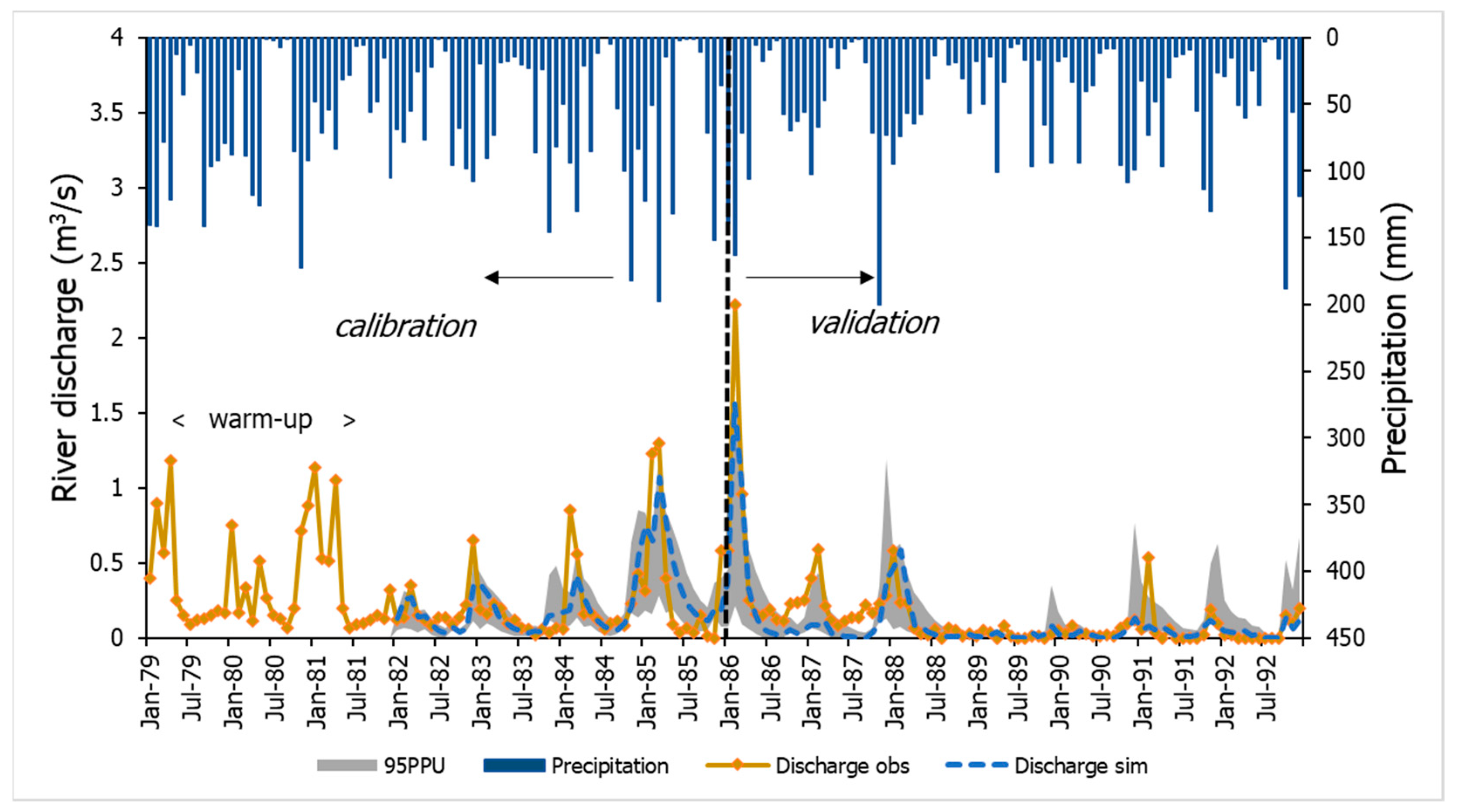
The comparison between the observed and simulated river discharge at Flumentepido gauge showed very good model performance reproducing the water balance in the watershed during validation (Figure 3). For the calibration period, the NSE, MSE, RMSE, and PBIAS values were 0.349, 0.050, 0.224, and 33.95, respectively (Table 3). For the validation period, the NSE, MSE, RMSE, and PBIAS values were 0.757, 0.019, 0.139, and 30.99, respectively (Table 2). According to Moriasi et al. [32], a streamflow simulation at monthly time step is considered very good if NSE > 0.75, and PBIAS < ± 10%, while RMSE being closer to zero indicates accurate model prediction. The unsatisfactory PBIAS value (>25%) could be explained by bias in some input and consequent some incorrect peak flow simulation during moderate rainfall events.
This effect was also reported in the literature for arid and semi-arid environments in Mediterranean climates [13,45]. The underestimation of major peak flow events could be explained by some errors in the meteorological data not uniformly distributed across the study area, as well as model limitations on reproducing complex processes that drive climate variability. Another possible explanation for prediction uncertainty is the complex geomorphology of the area and the proximity to the sea, which can limit both the performance of both baseline and climate projections performances.
The sensitivity analysis performed with the SWAT+ Toolbox showed that the most sensitive parameters that affect the simulation are: the baseflow recession constant (alpha); percolation coefficient (perco); minimum aquifer storage to allow return flow (flo_min); available water capacity of the soil layer (awc).
3.2. Future Climate and Water Balance Projections
For the assessment of future climate and water projections, the period 1979–2005 was considered as a baseline, while the future changes were estimated for up to 2050s (2006–2050) and 2098s (2051–2098), respectively. The results of projected changes for the main components of temperature, precipitation, and the water balance, under the climate models and RCP scenarios, are reported in Table 4, Table 5, Table 6, and Table 7. Supplementary data are presented in Tables S1–S6.
3.2.1. Projected Changes in Precipitation and Temperature
The mean annual precipitation under RCP4.5 and RCP8.5 scenarios project contrasting values for the RACMO22E model. Under the RCP4.5 during the mid-century, the projected precipitation was 474 mm/year (decrease by −25.4% compared to baseline), while during the late-century, a decrease equal to 456 mm/year (decrease by −28.3% compared to baseline) was estimated. Conversely, under the RCP8.5 scenario during the mid-century, the projected precipitation was 649 mm/year (decrease by −2% compared to baseline), while during the late-century, it was estimated equal to 647 mm/year (decrease by −1.7% compared to baseline). For the COSMO-CLM model under the RCP4.5 and RCP8.5, the precipitation projections indicate a slight increase (about 660 mm/year) for both emission scenarios for the mid-century and late-century.
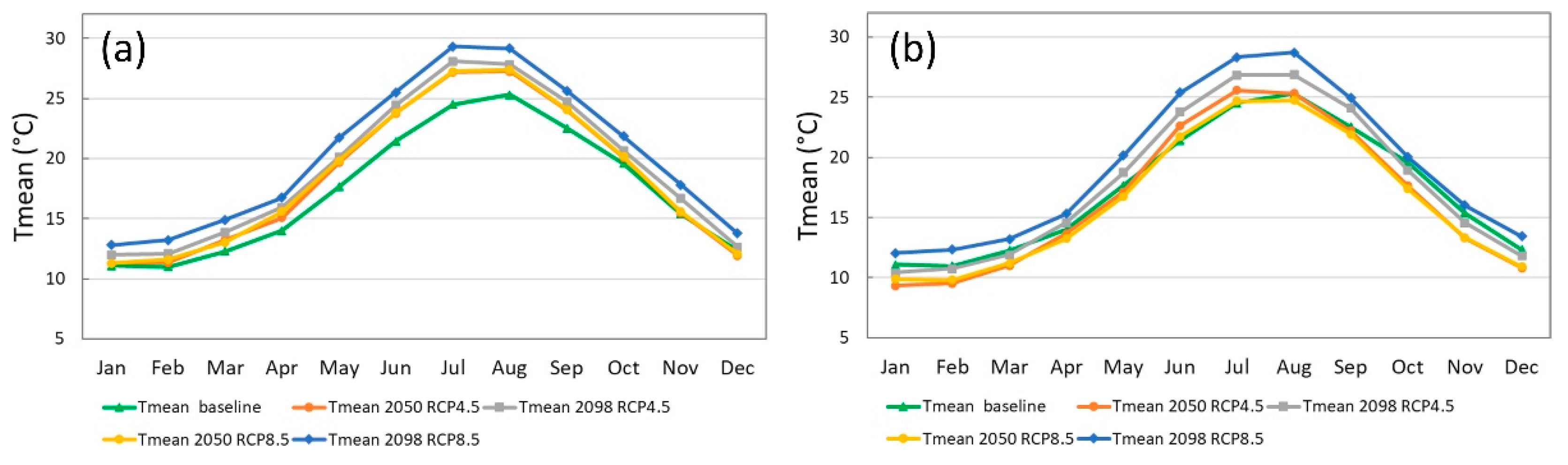
Concerning temperature, for the RACMO22E model, the mean annual temperature was projected to increase for both emission scenarios during the mid- and late-century (Figure 4). The highest increase is expected for the RCP8.5 emission scenario by 2.9 °C in the late-century compared to the baseline mean annual temperature. On a seasonal scale, July is the warmest month with a mean temperature and max temperature of 29.3 °C and 35.08 °C, respectively, under the RCP8.5 during the late-century (Table S2).
Temperatures for the COSMO-CLM model showed an increase during the late-century for both emission scenarios, with a maximum of 1.9 °C for the RCP8.5 as compared to the historically observed values. On a monthly scale, August is the warmest month with a mean temperature and max temperature of 28.7 °C and 33.1 °C, respectively, under the RCP8.5 during the late-century (Table S3). Overall, in contrast to predicted precipitation, both RCMs showed an increasing trend in temperatures, confirming general warming expected in Italy for the end of the century [34]. Simulations are not so large for median values, although the COSMO-CLM model tends to underestimate temperature, as suggested by other studies [33]. As suggested above for the baseline results, climate projections can be biased in areas with heterogeneous land cover, complex terrain, as well as with irregular coastlines [33]. Other researchers (see [46,47]) suggested that multiscale relations between climate phenomena and the streamflow could be rigorously analyzed in the future by the cross-wavelet analysis.
3.2.2. Projected Changes in Water Balance
At the basin scale, the mean annual potential evapotranspiration (PET) calculated with the Penman–Monteith equation was projected to increase significantly under both climate models compared to the baseline period equal to 1581 mm/year (Table 6 and Table 7). Under the RCP4.5 emission scenario for RACMO22E, PET was projected to increase up to 2201 mm/year and 2312 under the mid-century and late-century, respectively. Under the RCP8.5 scenario, PET has projected a further increase up to 2539 and 2763 mm/year under the mid-century and late-century, respectively.
PET is the dominant water balance component, and its increase is strongly driven by the increase in temperature. Conversely, actual evapotranspiration (ET) showed a decreasing trend during the summer months (Figure 4) since ET represents the real flow of water from the surface to the atmosphere, while PET is the evaporative demand of the atmosphere, mostly driven by temperature [13,48]. Data from several studies suggest similar increasing trends of PET in semi-arid climates [16,49]. The future increase in PET compared to the baseline in the basin is evident for both models and RCPs, as depicted on a monthly scale in Figure 4. In contrast, the ET trend is more uniform for both models and RCPs throughout the year.
The mean annual ET under the RCP4.5 scenario for RACMO22E showed a decrease during the mid-century (439 mm/year) (decrease by −19.3% compared to the baseline) and the late-century (425 mm/year) (decrease by −21.9% compared to the baseline) compared to the baseline period (544 mm/year). This decrease is consistent with the decrease in projected precipitation since these are a proxy for the ET trend, reflecting the exchange of energy in the soil-water-atmosphere processes [50]. On the contrary, under the RCP8.5 scenario, ET was projected to increase about 605 mm, following the increase in projected precipitation (both mid- and late-century) compared to the RCP4.5 scenario. On a monthly scale, the reduction in projected ET under the RCP4.5 was evident for the autumn months (Table S5 and Figure 5) due to a reduction in projected precipitation.
The total mean annual ET and PET for the COSMO-CLM model showed an increase during the late-century for both emission scenarios. Under the RCP4.5 scenario, PET has projected a further increase up to 2382 and 2563 mm/year under the mid-century and late-century, respectively. A less evident increase for the RCP8.5 scenario compared to RCP4.5, up to 2358 and 2675 mm/year under the mid-century and late-century, respectively. For the COSMO-CLM model, the projected annual ET remained almost constant for both scenarios during the mid-century and late-century (approximately 615 mm/year), an increase of 13% compared to the baseline period.
At the basin scale, the simulated water balance was projected to decrease for both scenarios due to increasing temperatures and the consequent amount of water loss in the atmosphere. Significant decreases are projected for total annual streamflow leaving the watershed (WYLD), surface runoff (SURQ), percolation (PERC), and lateral flow (LATQ) (Table 6 and Table 7). For the RACMO22E model, SURQ was projected with a marked reduction of 26.7 mm/year under the RCP4.5 scenario (decrease by −50% compared to the baseline period (54.3 mm/year), while the reduction under the RCP8.5 scenario is close to −40% compared to baseline period). Similarly, the COSMO-CLM model showed a decrease for SURQ of about 34 mm/year, a decrease of around −37% compared to the baseline period.
3.3. Consequences of Water Balance Alterations
In line with other climate change impacts on water balance over the Mediterranean region, this study found that the Sulcis area will experience a marked decrease of water components under the RCMs and emission scenarios in the future decades [13,51]. The reduction in precipitation and rising temperatures will alter flow regimes and consequently water availability at the watershed level [52,53,54]. Drought events, water stress, and temperature increases at the seasonal level will impact the growing cycle and phenological stages (e.g., flowering, ripening) of major crops, such as durum wheat, maize, vegetables, and forage production, impacting the quantity and quality of food production [55]. Mitigation scenarios and adaptation measures (e.g., early flowering and early sowing cultivars, new cultivars) toward climate-smart agriculture need to be addressed urgently to guarantee sustainable productions and economic benefits for local communities [3,56,57].
4. Conclusions
This study assesses the impacts of climate change on the hydrologic regime of a semi-arid Mediterranean watershed located in Sardinia (Italy) by using the restructured version of the Soil and Water Assessment Tool model. Simulation of the hydrological cycle was carried out by forcing the model with two RCMs for two emission scenarios (RCP4.5 and RCP8.5). The results show that by the end of the 21st century, climate change is projected to significantly affect water balance (i.e., water yield, groundwater recharge, baseflow, surface runoff). Therefore, these climate change effects on the hydrological regime might pose great challenges and further stress on agricultural crops in the study area, e.g., jeopardizing land use and irrigation practices.
Despite some inherent limitations of climate projections (e.g., accuracy, uncertainty) and specific methodological assumptions of the study (e.g., constant land use, constant agricultural management practices, and their role in the future flowrate conditions), the findings of this work can contribute to highlight possible consequences of future climate changes under the Mediterranean regions, as well as helping in designing high-resolution transformative adaptation on suitable water management, by providing insights for policymakers and decision-makers. From a further research perspective, the results of this study can be used to develop set-up detailed crop models and to define climate-smart agriculture practices and improved resources management.
Supplementary Materials
The following are available online at https://0-www-mdpi-com.brum.beds.ac.uk/article/10.3390/hydrology8040157/s1, Tables S1–S6.
Author Contributions
Conceptualization, G.P.; data curation, G.P.; methodology, G.P.; software, G.P.; validation, G.P.; formal analysis, G.P., F.L.; investigation, G.P.; writing—original draft preparation, G.P., F.L., H.C. and H.Y.; writing—review and editing, G.P., F.L., H.C. and H.Y.; visualization, G.P.; supervision, G.P. All authors have read and agreed to the published version of the manuscript.
Funding
This research received no external funding.
Institutional Review Board Statement
Not applicable.
Informed Consent Statement
Not applicable.
Data Availability Statement
The datasets generated during and/or analysed during the current study are available from the corresponding author on reasonable request.
Acknowledgments
We would like to thank Edoardo Bucchignani and CMCC Foundation (EuroMediterranean Centre on Climate Changes)—REMHI Division for providing the COSMO-CLM data. Thanks also to Juan José Sáenz de la Torre and Climadjust (https://climadjust.com/home (accessed on 30 May 2021)) for providing the RACMO22E data. Climadjust was funded by the Copernicus Climate Change Service and developed under contract C3S_428i.
Conflicts of Interest
The manuscript has no conflict of interests with Bayer CropScience.
Abbreviations
List of abbreviation: GCMs, General Circulation Models; RCMs, Regional Climate Models; SWAT, the Soil and Water Assessment Tool model; TOPKAPI, the TOPographic Kinematic APproximation and Integration model; RCPs, representative concentration pathways; HSPF, the Hydrological Simulation Program FORTRAN model; HRUs, Hydrologic Response Units; DEM, Digital Elevation Model; RAS, Autonomous Region of Sardinia; NSE, Nash-Sutcliffe efficiency; MSE, the mean square error; RMSE, the ratio of the root mean square error to the standard deviation; PBIAS, the percent of model bias; netCDF, network Common Data Form; COSMO-CLM, the climate model of the Centro Euro-Mediterraneo sui Cambiamenti Climatici; RACMO22E, the climate model of the Royal Netherlands Meteorological Institute; netCDF, Network Common Data Form file; CMIP5 CNRM-CM5, the Coupled Model Intercomparison Project of the National Centre for Meteorological Research; EURO-CORDEX, the European branch of the international CORDEX initiative; PET, potential evapotranspiration; ET, actual evapotranspiration. WYLD, water yield; SURQ, surface runoff; PERC, percolation; LATQ lateral flow.
References
- Ficklin, D.L.; Abatzoglou, J.T.; Robeson, S.M.; Null, S.E.; Knouft, J.H. Natural and managed watersheds show similar responses to recent climate change. Proc. Natl. Acad. Sci. USA 2018, 115, 8553–8557. [Google Scholar] [CrossRef] [PubMed] [Green Version]
- Pham, H.V.; Sperotto, A.; Torresan, S.; Acuña, V.; Jorda-Capdevila, D.; Rianna, G.; Marcomini, A.; Critto, A. Coupling scenarios of climate and land-use change with assessments of potential ecosystem services at the river basin scale. Ecosyst. Serv. 2019, 40, 101045. [Google Scholar] [CrossRef]
- Brouziyne, Y.; Abouabdillah, A.; Hirich, A.; Bouabid, R.; Zaaboul, R.; Benaabidate, L. Modeling sustainable adaptation strategies toward a climate-smart agriculture in a Mediterranean watershed under projected climate change scenarios. Agric. Syst. 2018, 162, 154–163. [Google Scholar] [CrossRef]
- Kahil, M.T.; Dinar, A.; Albiac, J. Modeling water scarcity and droughts for policy adaptation to climate change in arid and semiarid regions. J. Hydrol. 2015, 522, 95–109. [Google Scholar] [CrossRef] [Green Version]
- McConnell, L.L.; Kelly, I.D.; Jones, R.L. Integrating Technologies to Minimize Environmental Impacts. In Agricultural Chemicals and the Environment: Issues and Potential Solutions, 2nd ed.; Royal Society of Chemistry: London, UK, 2016; pp. 1–19. [Google Scholar]
- Aliyari, F.; Bailey, R.T.; Arabi, M. Appraising climate change impacts on future water resources and agricultural productivity in agro-urban river basins. Sci. Total Environ. 2021, 788, 147717. [Google Scholar] [CrossRef] [PubMed]
- Lionello, P.; Malanotte-Rizzoli, P.; Boscolo, R.; Alpert, P.; Artale, V.; Li, L.; Luterbacher, J.; May, W.; Trigo, R.; Tsimplis, M.; et al. The Mediterranean climate: An overview of the main characteristics and issues. In Developments in Earth and Environmental Sciences; Elsevier: Amsterdam, The Netherlands, 2006; pp. 1–26. [Google Scholar]
- Erol, A.; Randhir, T.O. Climatic change impacts on the ecohydrology of Mediterranean watersheds. Clim. Chang. 2012, 114, 319–341. [Google Scholar] [CrossRef]
- Alessandri, A.; De Felice, M.; Zeng, N.; Mariotti, A.; Pan, Y.; Cherchi, A.; Lee, J.-Y.; Wang, B.; Ha, K.-J.; Ruti, P.; et al. Robust assessment of the expansion and retreat of Mediterranean climate in the 21st century. Sci. Rep. 2015, 4, 7211. [Google Scholar] [CrossRef]
- Schär, C.; Vidale, P.L.; Lüthi, D.; Frei, C.; Häberli, C.; Liniger, M.A.; Appenzeller, C. The role of increasing temperature variability in European summer heatwaves. Nature 2004, 427, 332–336. [Google Scholar] [CrossRef] [PubMed]
- Mastrantonas, N.; Herrera-Lormendez, P.; Magnusson, L.; Pappenberger, F.; Matschullat, J. Extreme precipitation events in the Mediterranean: Spatiotemporal characteristics and connection to large-scale atmospheric flow patterns. Int. J. Climatol. 2021, 41, 2710–2728. [Google Scholar] [CrossRef]
- Leta, O.T.; Bauwens, W. Assessment of the impact of climate change on daily extreme peak and low flows of Zenne basin in Belgium. Hydrology 2018, 5, 38. [Google Scholar] [CrossRef] [Green Version]
- Brouziyne, Y.; De Girolamo, A.M.; Aboubdillah, A.; Benaabidate, L.; Bouchaou, L.; Chehbouni, A. Modeling alterations in flow regimes under changing climate in a Mediterranean watershed: An analysis of ecologically-relevant hydrological indicators. Ecol. Inform. 2021, 61, 101219. [Google Scholar] [CrossRef]
- Vezzoli, R.; Mercogliano, P.; Pecora, S.; Zollo, A.L.; Cacciamani, C. Hydrological simulation of Po River (North Italy) discharge under climate change scenarios using the RCM COSMO-CLM. Sci. Total Environ. 2015, 521–522, 346–358. [Google Scholar] [CrossRef]
- Meinshausen, M.; Smith, S.J.; Calvin, K.; Daniel, J.S.; Kainuma, M.L.T.; Lamarque, J.; Matsumoto, K.; Montzka, S.A.; Raper, S.C.B.; Riahi, K.; et al. The RCP greenhouse gas concentrations and their extensions from 1765 to 2300. Clim. Change 2011, 109, 213–241. [Google Scholar] [CrossRef] [Green Version]
- Fonseca, A.R.; Santos, J.A. Predicting hydrologic flows under climate change: The Tâmega Basin as an analog for the Mediterranean region. Sci. Total Environ. 2019, 668, 1013–1024. [Google Scholar] [CrossRef]
- Arnold, J.G.; Moriasi, D.N.; Gassman, P.W.; Abbaspour, K.C.; White, M.J.; Srinivasan, R.; Santhi, C.; Harmel, R.D.; van Griensven, A.; Van Liew, M.W.; et al. SWAT: Model Use, Calibration, and Validation. Trans. ASABE 2012, 55, 1491–1508. [Google Scholar] [CrossRef]
- Wang, R.; Yuan, Y.; Yen, H.; Grieneisen, M.; Arnold, J.; Wang, D.; Wang, C.; Zhang, M. A review of pesticide fate and transport simulation at watershed level using SWAT: Current status and research concerns. Sci. Total Environ. 2019, 669, 512–526. [Google Scholar] [CrossRef]
- Gassman, P.W.; Sadeghi, A.M.; Srinivasan, R. Applications of the SWAT Model Special Section: Overview and Insights. J. Environ. Qual. 2014, 43, 1–8. [Google Scholar] [CrossRef]
- van Tol, J.; Bieger, K.; Arnold, J.G. A hydropedological approach to simulate streamflow and soil water contents with SWAT+. Hydrol. Process. 2021, 35. [Google Scholar] [CrossRef]
- Bieger, K.; Arnold, J.G.; Rathjens, H.; White, M.J.; Bosch, D.D.; Allen, P.M.; Volk, M.; Srinivasan, R. Introduction to SWAT+, A Completely Restructured Version of the Soil and Water Assessment Tool. JAWRA J. Am. Water Resour. Assoc. 2017, 53, 115–130. [Google Scholar] [CrossRef]
- Tan, M.L.; Gassman, P.W.; Yang, X.; Haywood, J. A review of SWAT applications, performance and future needs for simulation of hydro-climatic extremes. Adv. Water Resour. 2020, 143, 103662. [Google Scholar] [CrossRef]
- Pulighe, G.; Bonati, G.; Colangeli, M.; Traverso, L.; Lupia, F.; Altobelli, F.; Marta, A.D.; Napoli, M. Predicting streamflow and nutrient loadings in a semi-arid Mediterranean watershed with ephemeral streams using the SWAT model. Agronomy 2020, 10, 2. [Google Scholar] [CrossRef] [Green Version]
- Ricci, G.F.; De Girolamo, A.M.; Abdelwahab, O.M.M.; Gentile, F. Identifying sediment source areas in a Mediterranean watershed using the SWAT model. L. Degrad. Dev. 2018, 29, 1233–1248. [Google Scholar] [CrossRef]
- Panagopoulos, Y.; Makropoulos, C.; Baltas, E.; Mimikou, M. SWAT parameterization for the identification of critical diffuse pollution source areas under data limitations. Ecol. Modell. 2011, 222, 3500–3512. [Google Scholar] [CrossRef]
- Chen, Y.; Marek, G.W.; Marek, T.H.; Moorhead, J.E.; Heflin, K.R.; Brauer, D.K.; Gowda, P.H.; Srinivasan, R. Simulating the impacts of climate change on hydrology and crop production in the Northern High Plains of Texas using an improved SWAT model. Agric. Water Manag. 2019, 221, 13–24. [Google Scholar] [CrossRef]
- QGIS Geographic Information System. QGIS Development Team. Available online: https://www.qgis.org/it/site/ (accessed on 30 September 2021).
- RAS Regione Autonoma della Sardegna—Sardegna Geoportale. Available online: http://www.sardegnageoportale.it/index.php?xsl=1594&s=40&v=9&c=8753&n=10 (accessed on 30 May 2021).
- CFSR, The National Centers for Environmental Prediction (NCEP)–Climate Forecast System Reanalysis (CFSR), 2019. Available online: https://www.ncei.noaa.gov/products/weather-climate-models/climate-forecast-system (accessed on 30 May 2021).
- SWAT+. Introducing SWAT+, A Completely Revised Version of the SWAT Model. Available online: https://swat.tamu.edu/software/plus/ (accessed on 30 September 2021).
- Moriasi, D.N.; Arnold, J.G.; Van Liew, M.W.; Bingner, R.L.; Harmel, R.D.; Veith, T.L. Model evaluation guidelines for systematic quantification of accuracy in watershed simulations. Trans. ASABE 2007, 50, 885–900. [Google Scholar] [CrossRef]
- RAS Regione Autonoma della Sardegna—Annali Idrologici Della Sardegna. Available online: https://www.regione.sardegna.it/j/v/25?s=205270&v=2&c=5650&t=1 (accessed on 10 May 2021).
- Zollo, A.L.; Rillo, V.; Bucchignani, E.; Montesarchio, M.; Mercogliano, P. Extreme temperature and precipitation events over Italy: Assessment of high-resolution simulations with COSMO-CLM and future scenarios. Int. J. Climatol. 2016, 36, 987–1004. [Google Scholar] [CrossRef] [Green Version]
- Bucchignani, E.; Montesarchio, M.; Zollo, A.L.; Mercogliano, P. High-resolution climate simulations with COSMO-CLM over Italy: Performance evaluation and climate projections for the 21st century. Int. J. Climatol. 2016, 36, 735–756. [Google Scholar] [CrossRef]
- Bonfante, A.; Monaco, E.; Langella, G.; Mercogliano, P.; Bucchignani, E.; Manna, P.; Terribile, F. A dynamic viticultural zoning to explore the resilience of terroir concept under climate change. Sci. Total Environ. 2018, 624, 294–308. [Google Scholar] [CrossRef]
- Adinolfi, M.; Raffa, M.; Reder, A.; Mercogliano, P. Evaluation and expected changes of summer precipitation at convection permitting scale with COSMO-CLM over alpine space. Atmosphere 2021, 12, 54. [Google Scholar] [CrossRef]
- Senatore, A.; Mendicino, G.; Smiatek, G.; Kunstmann, H. Regional climate change projections and hydrological impact analysis for a Mediterranean basin in Southern Italy. J. Hydrol. 2011, 399, 70–92. [Google Scholar] [CrossRef]
- van Meijgaard, E.; van Ulft, L.H.; van de Berg, W.J.; Bosveld, F.C.; van den Hurk, B.J.J.M.; Lenderink, G.; Siebesma, A.P. The KNMI Regional Atmospheric Climate Model RACMO Version 2.1; KNMI: De Bilt, The Netherlands, 2008. [Google Scholar]
- EURO-CORDEX Coordinated Downscaling Experiment—European Domain. Available online: https://www.euro-cordex.net/ (accessed on 30 September 2021).
- Climadjust. Climadjust Was Funded by the Copernicus Climate Change Service and Developed under Contract C3S_428i. Available online: https://climadjust.com/home (accessed on 10 March 2021).
- Vautard, R.; Kadygrov, N.; Iles, C.; Boberg, F.; Buonomo, E.; Bülow, K.; Coppola, E.; Corre, L.; Meijgaard, E.; Nogherotto, R.; et al. Evaluation of the large EURO-CORDEX regional climate model ensemble. J. Geophys. Res. Atmos. 2020, 26, 1–28. [Google Scholar]
- Thomson, A.M.; Calvin, K.V.; Smith, S.J.; Kyle, G.P.; Volke, A.; Patel, P.; Delgado-Arias, S.; Bond-Lamberty, B.; Wise, M.A.; Clarke, L.E.; et al. RCP4.5: A pathway for stabilization of radiative forcing by 2100. Clim. Chang. 2011, 109, 77–94. [Google Scholar] [CrossRef] [Green Version]
- van Vuuren, D.P.; Edmonds, J.; Kainuma, M.; Riahi, K.; Thomson, A.; Hibbard, K.; Hurtt, G.C.; Kram, T.; Krey, V.; Lamarque, J.F.; et al. The representative concentration pathways: An overview. Clim. Chang. 2011, 109, 5–31. [Google Scholar] [CrossRef]
- Hausfather, Z.; Peters, G.P. Emissions—The ‘business as usual’ story is misleading. Nature 2020, 577, 618–620. [Google Scholar] [CrossRef]
- Chen, H.; Luo, Y.; Potter, C.; Moran, P.J.; Grieneisen, M.L.; Zhang, M. Modeling pesticide diuron loading from the San Joaquin watershed into the Sacramento-San Joaquin Delta using SWAT. Water Res. 2017, 121, 374–385. [Google Scholar] [CrossRef]
- Ghaderpour, E.; Vujadinovic, T.; Hassan, Q.K. Application of the Least-Squares Wavelet software in hydrology: Athabasca River Basin. J. Hydrol. Reg. Stud. 2021, 36, 100847. [Google Scholar] [CrossRef]
- Canchala, T.; Loaiza Cerón, W.; Francés, F.; Carvajal-Escobar, Y.; Andreoli, R.; Kayano, M.; Alfonso-Morales, W.; Caicedo-Bravo, E.; Ferreira de Souza, R. Streamflow Variability in Colombian Pacific Basins and Their Teleconnections with Climate Indices. Water 2020, 12, 526. [Google Scholar] [CrossRef] [Green Version]
- Donohue, R.J.; McVicar, T.R.; Roderick, M.L. Assessing the ability of potential evaporation formulations to capture the dynamics in evaporative demand within a changing climate. J. Hydrol. 2010, 386, 186–197. [Google Scholar] [CrossRef]
- Mengistu, D.; Bewket, W.; Dosio, A.; Panitz, H.J. Climate change impacts on water resources in the Upper Blue Nile (Abay) River Basin, Ethiopia. J. Hydrol. 2021, 592, 125614. [Google Scholar] [CrossRef]
- Allen, R.G.; Pereira, L.S.; Raes, D.; Smith, M. FAO Irrigation and Drainage Paper N.56. Crop. Evapotranspiration—Guidelines for Computing Crop Water Requirements; FAO Irrigation and drainage paper 56; FAO: Rome, Italy, 1998; ISBN 9251042195. [Google Scholar]
- Giannakopoulos, C.; Le Sager, P.; Bindi, M.; Moriondo, M.; Kostopoulou, E.; Goodess, C.M. Climatic changes and associated impacts in the Mediterranean resulting from a 2 °C global warming. Glob. Planet. Chang. 2009, 68, 209–224. [Google Scholar] [CrossRef]
- Spinoni, J.; Vogt, J.V.; Naumann, G.; Barbosa, P.; Dosio, A. Will drought events become more frequent and severe in Europe? Int. J. Climatol. 2018, 38, 1718–1736. [Google Scholar] [CrossRef] [Green Version]
- Milano, M.; Ruelland, D.; Fernandez, S.; Dezetter, A.; Fabre, J.; Servat, E.; Fritsch, J.-M.; Ardoin-Bardin, S.; Thivet, G. Current state of Mediterranean water resources and future trends under climatic and anthropogenic changes. Hydrol. Sci. J. 2013, 58, 498–518. [Google Scholar] [CrossRef]
- Saade, J.; Atieh, M.; Ghanimeh, S.; Golmohammadi, G. Modeling Impact of Climate Change on Surface Water Availability Using SWAT Model in a Semi-Arid Basin: Case of El Kalb River, Lebanon. Hydrology 2021, 8, 134. [Google Scholar] [CrossRef]
- Yang, C.; Fraga, H.; van Ieperen, W.; Trindade, H.; Santos, J.A. Effects of climate change and adaptation options on winter wheat yield under rainfed Mediterranean conditions in southern Portugal. Clim. Chang. 2019, 154, 159–178. [Google Scholar] [CrossRef] [Green Version]
- Iglesias, A.; Garrote, L. Adaptation strategies for agricultural water management under climate change in Europe. Agric. Water Manag. 2015, 155, 113–124. [Google Scholar] [CrossRef] [Green Version]
- Garrote, L.; Granados, A.; Iglesias, A. Strategies to reduce water stress in Euro-Mediterranean river basins. Sci. Total Environ. 2016, 543, 997–1009. [Google Scholar] [CrossRef]
Figure 1.
Location of the Sulcis area with respect to Italy (a) and Sardinia (b). The map shows the river network and the location of the gauge station.
Figure 1.
Location of the Sulcis area with respect to Italy (a) and Sardinia (b). The map shows the river network and the location of the gauge station.

Figure 2.
The main steps for setting-up the SWAT+ model, conducting calibration/validation, and climate change scenarios.
Figure 2.
The main steps for setting-up the SWAT+ model, conducting calibration/validation, and climate change scenarios.

Figure 3.
Precipitation and simulated and observed monthly discharges during the calibration and validation periods at the Flumentepido gauge station. Prediction uncertainty 95% (95PPU).
Figure 3.
Precipitation and simulated and observed monthly discharges during the calibration and validation periods at the Flumentepido gauge station. Prediction uncertainty 95% (95PPU).

Figure 4.
Monthly evolution of the mean temperature for: (a) RACMO22E under the RCP4.5 and RCP8.5; (b) COSMO-CLM under the RCP4.5 and RCP8.5.
Figure 4.
Monthly evolution of the mean temperature for: (a) RACMO22E under the RCP4.5 and RCP8.5; (b) COSMO-CLM under the RCP4.5 and RCP8.5.

Figure 5.
Monthly evolution of precipitation, actual evapotranspiration, and potential evapotranspiration for: RACMO22E under the RCP4.5 (a) and RCP8.5 (b); COSMO-CLM under the RCP4.5 (c) and RCP8.5 (d).
Figure 5.
Monthly evolution of precipitation, actual evapotranspiration, and potential evapotranspiration for: RACMO22E under the RCP4.5 (a) and RCP8.5 (b); COSMO-CLM under the RCP4.5 (c) and RCP8.5 (d).

Table 3.
Calibration and validation performance of the SWAT+ model at the Flumentepido river gauge station.
Table 3.
Calibration and validation performance of the SWAT+ model at the Flumentepido river gauge station.
| Objective Functions | Calibration | Validation |
|---|---|---|
| NSE | 0.349 | 0.757 |
| MSE | 0.050 | 0.019 |
| RMSE | 0.224 | 0.139 |
| PBIAS | 33.95 | 30.99 |
Table 4.
Precipitation and temperature under baseline and future climate projections for the RACMO22E regional climate model under RCP4.5 and RCP8.5 scenarios.
Table 4.
Precipitation and temperature under baseline and future climate projections for the RACMO22E regional climate model under RCP4.5 and RCP8.5 scenarios.
| Baseline | 2006–2050 (RCP4.5) | 2051–2098 (RCP4.5) | 2006–2050 (RCP8.5) | 2051–2098 (RCP8.5) | |
|---|---|---|---|---|---|
| Precipitation (mm/year) | 639 | 474 | 456 | 649 | 647 |
| Temp max (°C) | 20.2 | 22.6 | 23.3 | 22.7 | 24.4 |
| Temp min (°C) | 14.4 | 14.2 | 15 | 14.3 | 16.1 |
| Temp mean (°C) | 17.3 | 18.4 | 19.1 | 18.5 | 20.2 |
Table 5.
Precipitation and temperature under baseline and future climate projections for the COSMO-CLM regional climate model under RCP4.5 and RCP8.5 scenarios.
Table 5.
Precipitation and temperature under baseline and future climate projections for the COSMO-CLM regional climate model under RCP4.5 and RCP8.5 scenarios.
| Baseline | 2006–2050 (RCP4.5) | 2051–2098 (RCP4.5) | 2006–2050 (RCP8.5) | 2051–2098 (RCP8.5) | |
|---|---|---|---|---|---|
| Precipitation (mm/year) | 639 | 664 | 663 | 662 | 662 |
| Temp max (°C) | 20.2 | 20.2 | 21.5 | 19.8 | 22.7 |
| Temp min (°C) | 14.4 | 12.9 | 14.2 | 12.9 | 15.7 |
| Temp mean (°C) | 17.3 | 16.6 | 17.8 | 16.3 | 19.2 |
Table 6.
Water balance components under baseline and future climate projections for the RACMO22E regional climate model under RCP4.5 and RCP8.5 scenarios.
Table 6.
Water balance components under baseline and future climate projections for the RACMO22E regional climate model under RCP4.5 and RCP8.5 scenarios.
| (mm/year) | Baseline | 2006–2050 (RCP4.5) | 2051–2098 (RCP4.5) | 2006–2050 (RCP8.5) | 2051–2098 (RCP8.5) |
|---|---|---|---|---|---|
| PET | 1581 | 2201 | 2312 | 2539 | 2763 |
| ET | 544 | 439 | 425 | 605 | 604 |
| SURQ | 54.3 | 26.7 | 23.9 | 33.7 | 32.5 |
| LATQ | 6.13 | 2.12 | 1.89 | 2.71 | 2.59 |
| PERC | 31.1 | 6.67 | 5.75 | 8.8 | 8.19 |
| WYLD | 60.4 | 28.8 | 25.8 | 36.4 | 35.1 |
Table 7.
Water balance components under baseline and future climate projections for the COSMO-CLM regional climate model under RCP4.5 and RCP8.5 scenarios.
Table 7.
Water balance components under baseline and future climate projections for the COSMO-CLM regional climate model under RCP4.5 and RCP8.5 scenarios.
| (mm/Year) | Baseline | 2006–2050 (RCP4.5) | 2051–2098 (RCP4.5) | 2006–2050 (RCP8.5) | 2051–2098 (RCP8.5) |
|---|---|---|---|---|---|
| PET | 1581 | 2382 | 2563 | 2358 | 2675 |
| ET | 544 | 614 | 618 | 613 | 615 |
| SURQ | 54.3 | 36.2 | 34.7 | 34.8 | 34.2 |
| LATQ | 6.13 | 3.02 | 2.52 | 2.78 | 2.61 |
| PERC | 31.1 | 10.5 | 7.85 | 8.91 | 8.56 |
| WYLD | 60.4 | 39.2 | 37.2 | 37.6 | 36.8 |
Publisher’s Note: MDPI stays neutral with regard to jurisdictional claims in published maps and institutional affiliations. |
© 2021 by the authors. Licensee MDPI, Basel, Switzerland. This article is an open access article distributed under the terms and conditions of the Creative Commons Attribution (CC BY) license (https://creativecommons.org/licenses/by/4.0/).
Share and Cite
MDPI and ACS Style
Pulighe, G.; Lupia, F.; Chen, H.; Yin, H. Modeling Climate Change Impacts on Water Balance of a Mediterranean Watershed Using SWAT+. Hydrology 2021, 8, 157. https://0-doi-org.brum.beds.ac.uk/10.3390/hydrology8040157
AMA Style
Pulighe G, Lupia F, Chen H, Yin H. Modeling Climate Change Impacts on Water Balance of a Mediterranean Watershed Using SWAT+. Hydrology. 2021; 8(4):157. https://0-doi-org.brum.beds.ac.uk/10.3390/hydrology8040157
Chicago/Turabian StylePulighe, Giuseppe, Flavio Lupia, Huajin Chen, and Hailong Yin. 2021. "Modeling Climate Change Impacts on Water Balance of a Mediterranean Watershed Using SWAT+" Hydrology 8, no. 4: 157. https://0-doi-org.brum.beds.ac.uk/10.3390/hydrology8040157
Note that from the first issue of 2016, this journal uses article numbers instead of page numbers. See further details here.