3.1. Water Quality Evaluation
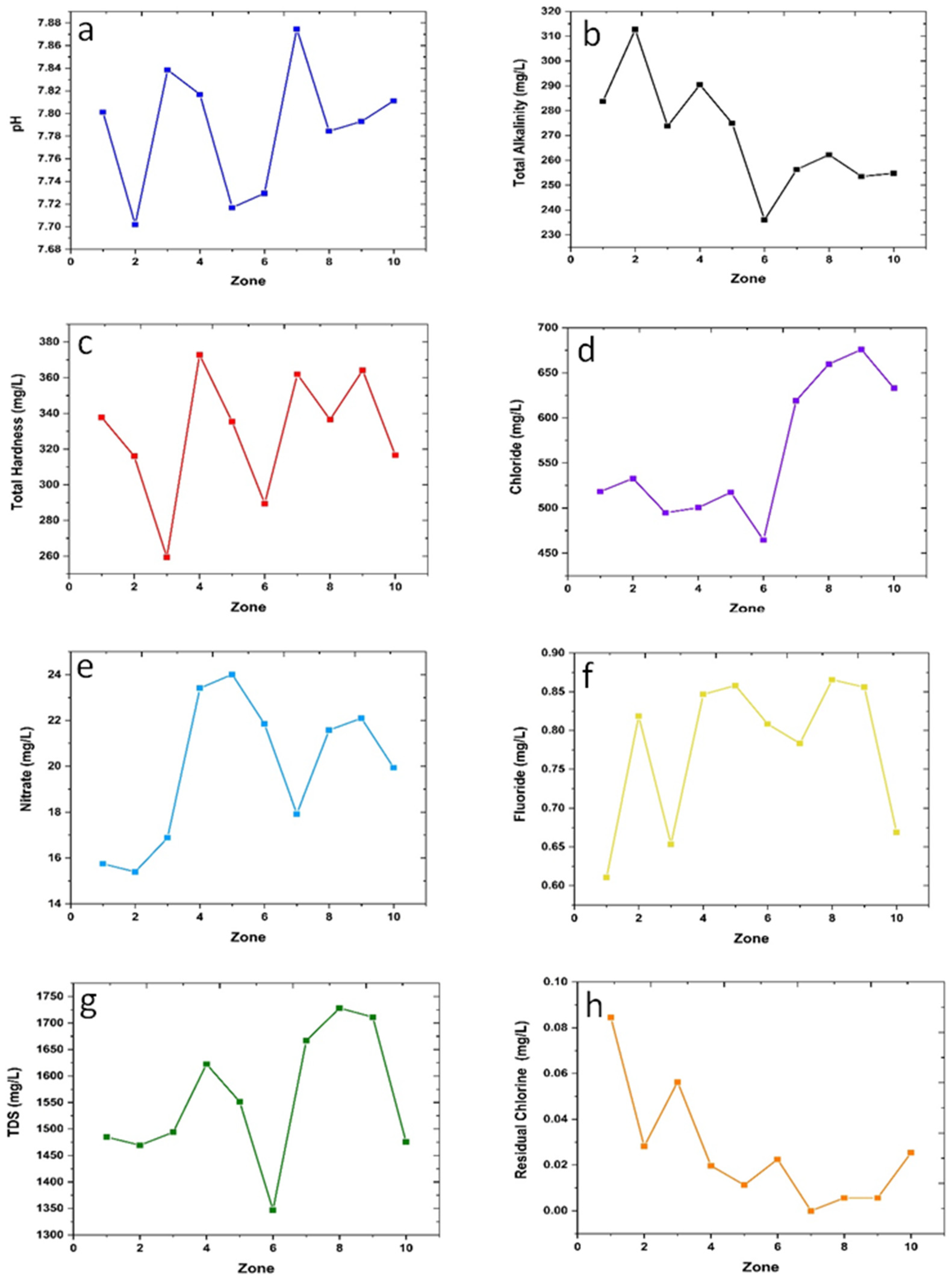
Figure 2a–h shows the variation of average values of various water quality parameters as a function of locations; the zones were selected arbitrarily and did not represent any well-defined functional relation with distance or other geographic or demographic parameters. Thus, the results shown in
Figure 2a–h indicate that the quality parameters vary from place to place. It can be observed that there is considerable variation in the magnitude of average values of each quality parameter across the selected zones. In
Figure 2a, it is revealed that the pH value is different in different zones, and its value lies within a range from 7.70 to 7.88 and hence is higher than the most desirable value of pH, which is 7. Similarly, another parameter, viz., total alkalinity (TA), is seen to have varied from 236.06 mg/L to 312.68 mg/L as shown in
Figure 2b. The range of variation of the average values of the other water quality parameters can be seen to vary within the ranges, such as TH (259.30 mg/L to 372.82 mg/L), chloride (464.507 mg/L to 675.775 mg/L), nitrate (15.39 mg/L to 24.01 mg/L), fluoride (0.61 mg/L to 0.87 mg/L), TDS (1347.04 mg/L to 1728.31 mg/L), and residual chlorine (0–0.01); the variations are shown in
Figure 2c–h, respectively. It is important to note that the TDS of water in Jodhpur is much higher than the desired value, ~less than 500 mg/L. However, in water-stressed regions, the higher value (2000 mg/L) is accepted as per the BIS standard; suitable TDS removal techniques may be adopted in such cases. It should be reiterated that ideally the TDS must be kept below 500 mg/L; although in a water-stressed region such as the Jodhpur district of Rajasthan, India, one may make use of higher TDS water. However, TDS removal techniques are quite simple, especially with solar energy. Normally, hotter areas are water-stressed (e.g., California, USA) and in most cases, one would come across high TDS water; to make water abundantly available for drinking; the simpler solar heating technique may be applied, or even boiling the water will reduce the TDS level. Considering this, we took 500 mg/L as the lower limit and 2000 mg/L as the higher limit of acceptance. Admittedly, a TDS value less than the permissible value as per the BIS standard (500 mg/L) is always better. In the present case, we took 500 mg/L to be the most desirable value which can be comfortably set as the lower limit of acceptance without regard to the beneficial consequences for the case of still lower TDS values. Moreover, it was also recognized that a zero TDS value must not index the best quality with respect to the TDS value.
Similarly, a threshold value of 0.2 was set as the acceptable lower limit for chlorine. In cases where its value goes below this threshold, it may present a health concern. Similarly, for fluoride, the lower limit was taken to be 1, notwithstanding if a lower fluoride level is good for health. Noting that the average of 71 samples from a zone varied with the location of the zones, it seemed wise to examine if the average of the zonal averages of each parameter can bear significance in determining the overall quality of drinking water for the entire region.
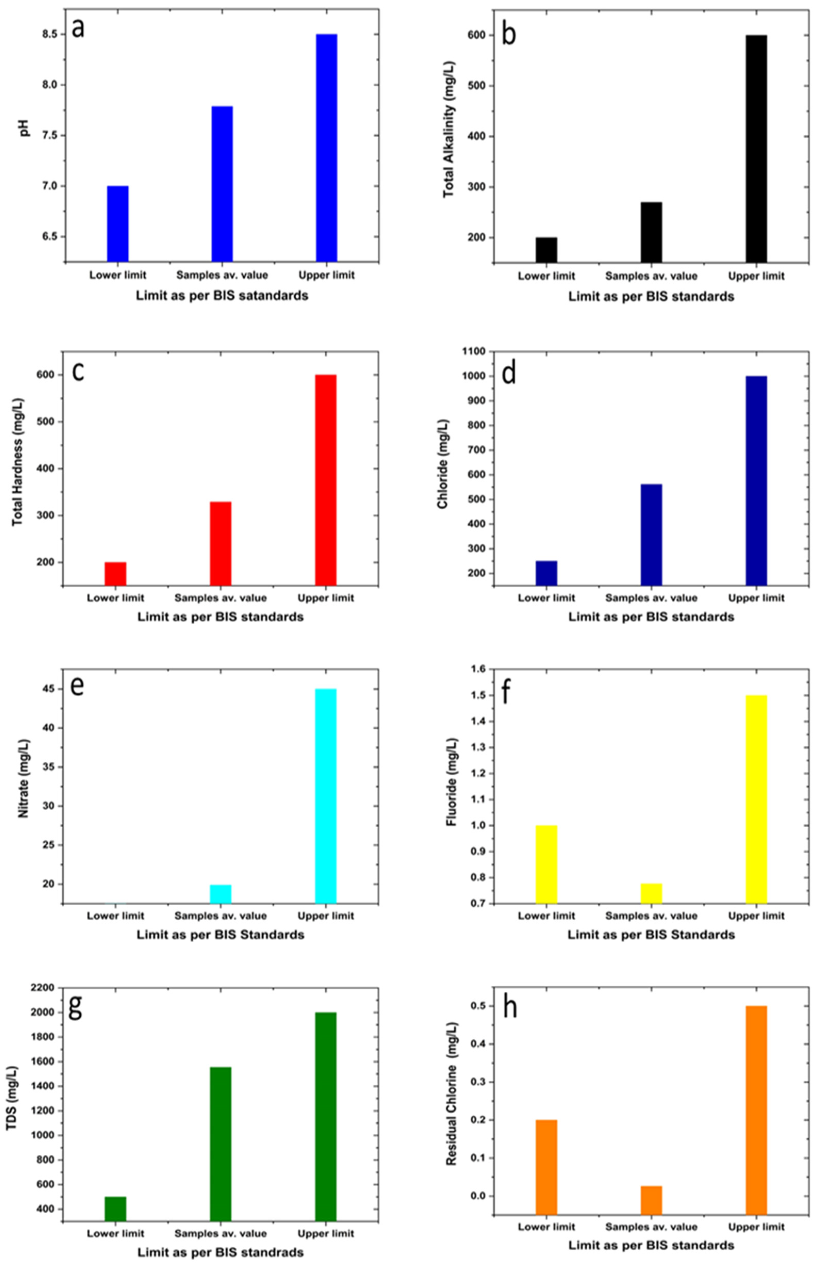
The overall average value of each water quality parameter for the entire region was obtained by taking the average of the individual quality average for each zone; the value of each parameter in a zone was essentially the average of 71 samples belonging to the concerned zone. Such a global average of each quality parameter is presented in
Figure 2. The same figure also shows acceptable ranges of parametric values as stipulated by BIS (
Table 1). The bar chart in
Figure 3 shows the acceptable lower limit of a parameter as well as its upper limit of acceptance. It is apparent from
Figure 3a that the regional average value of pH was higher than the acceptable lower limit of the pH value for potable water, whereas it lies below the upper allowable limit in respect to the specification laid down by BIS (
Table 1). Similarly, average values of other parameters such as TA, TH, Cl, nitrate, fluoride, TDS, and residual chlorine were also mapped in the form of similar bar diagrams and are shown in
Figure 3b–h. From
Figure 3, it can be observed that the global average values for all the tested water quality parameters (eight in number) lie within their acceptable minimum and maximum values as per the BIS recommendation. When the value of a water quality parameter (as given by the average of 710 samples, divided into groups with 71 samples each) is found to be less than the permissible minimum or higher than the maximum permissible value as per specifications, it attracts attention from the users’ side. It may be noted that the closeness of the average of a parameter towards the lower limit is different for different parameters; if we presume that the closer the value of a parameter is to the lower limit of acceptance, the better is the water quality in respect to the concerned parameter, it becomes apparent that individual quality parameters have different goodness of quality. This leads one to think of adopting a rational approach to describing the overall quality of water by linking the quality goodness of individual parameters. Incidentally, pH is somewhat an exception as it is universally accepted that a value of 7 represents the best pH value desirable in drinking water. However, there are other important water quality parameters, some of which are known to directly impact the pH value. So, to rationalize the parametric contribution to determining the overall quality of drinking water, the lower limit acceptance of a specific quality parameter is considered its best possible quality goodness. In this respect, a pH value of 7.0 is taken to be the acceptable lower limit. It may be noted that there are other parameters that affect the water quality, for example, BOD, COD, dissolved oxygen, total coliform, and conductivity. In fact, there has been a report on water quality modeling using an ANN wherein as many as 56 input nodes were used [
23]. With the aim to forecast algal growth in Tolo Harbour, Hongkong, Deng et al. [
23] used an ANN of structure, [56]
input-1-[1]
output, and modeling was carried out in MATLAB. With four different algorithms, a learning rate of 0.01 and training epoch of 1000 was used to achieve better predictive power. Another machine learning (ML) technique, support vector machine (SVM), was also used to find out the suitability of a technique with respect to the forecasting capability [
23]. RMSE and correlation coefficient R-values were used to judge the performance of various options. The performance of the SVM was better than that of the ANN, but with a higher computation time; of the different algorithms used in the ANN, the performance of the Levenberg–Marquardt (LM) algorithm was found to be superior. However, the present work deals with the formulation of the quality index of potable water. Though more input parameters, including those stated above, could have been used in the modeling, we felt it prudent to validate the conceived model with the use of these eight parameters, which appear to be quite important with respect to sensitivity towards determining the quality of drinking water. The use of more parameters would have given rise to a different result and could possibly be related to the drinkability of water. However, in that case, much more complexity would be involved in modeling as many of the parameters could have been found to be insignificant. Notwithstanding the experimental limitations, it would be an interesting exercise to model those parameters as well, and this work may be taken up as a separate study.
Accepting that different quality parameters have different goodness, it seems worth seeking a unique stochastic token that can describe the combined effect of all the water quality parameters and give the best idea for the quality of drinking water. In line with previous work, we propose defining such a stochastic token as a ‘water quality index’ (WQI) [
24].
From the results in
Table 2, the cumulative average values of each quality variable for the entire region are calculated by taking the average of the zonal average values of individual water quality parameters. Thus, the net average value of a quality parameter is equal to the sum of the average value of a parameter for each zone/total number of zones. Based on these derived average values, a simple algorithm is proposed to evaluate the individual parameter’s net quality index; taking the individual parameter’s quality index into consideration, the overall water quality index for the concerned region is described.
3.2. Water Quality Index
The present proposition of designing the water quality index for the Jodhpur region aims to qualify the degree of goodness of drinking water on a scale of 0–100. A value of 100 is obtainable for a parameter only if its average value equals the set lower limit, notwithstanding the achievable betterness below the set lower limit, which is called the permissible limit in the BIS standard. The measured data reveals that there is little scope to fix any other lower limit below the so-called permissible limit.
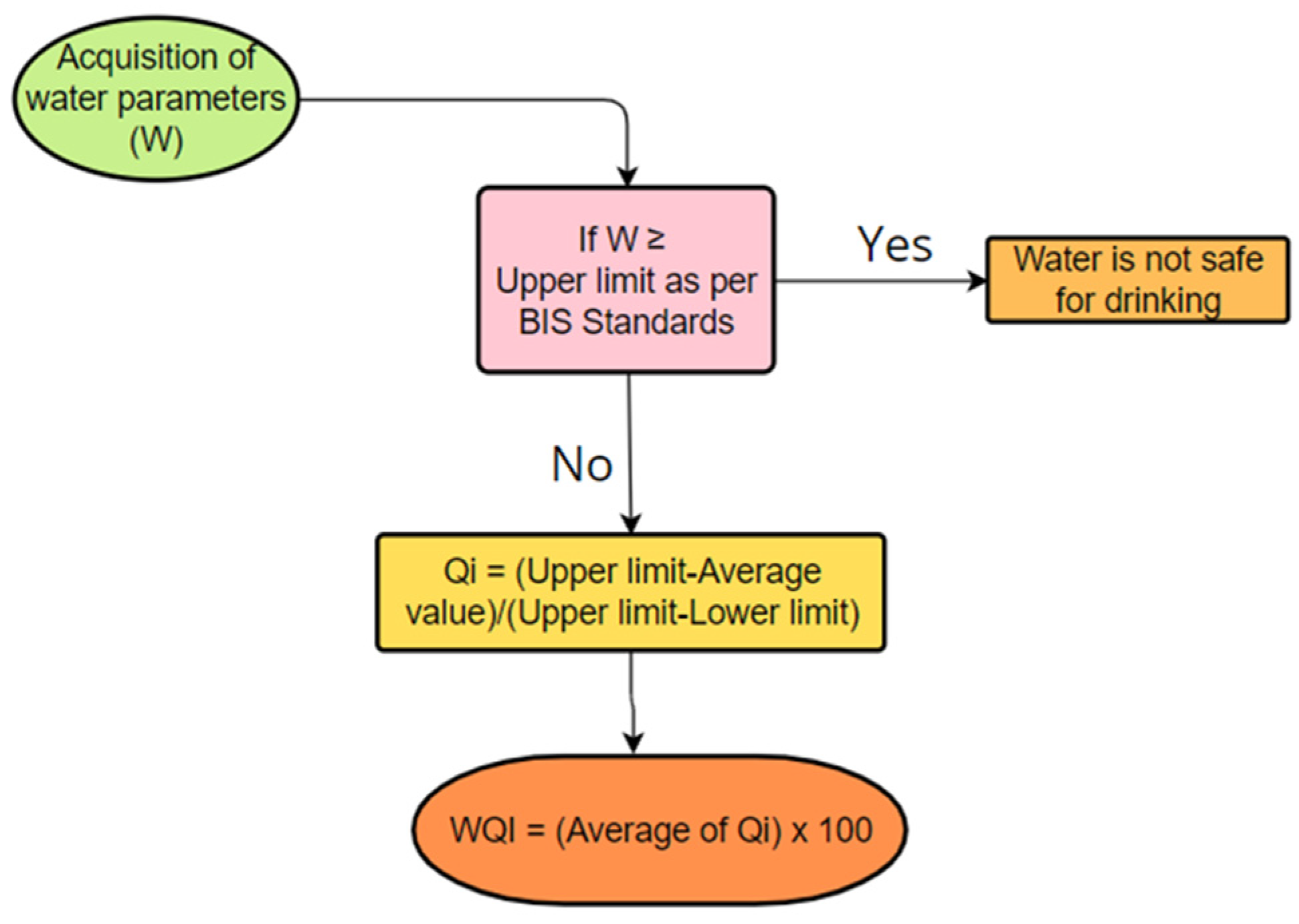
The following algorithm is proposed for determining the water quality index of the chosen region in consideration of the results of 710 water samples tests, as carried out in the present research work (
Figure 4). To accomplish this, the following assumptions are made:
The acceptable lower and upper limit of quality parameters for use in the study are selected with an eye to the scope available in the BIS standard.
Within a given range of specifications, the closer the average value (of a quality parameter) lies to the acceptable lower limit (
Table 2), the higher the parametric quality index will be.
If the minimum accepted value is not specified in a standard, the acceptable lower limit shall be considered zero.
The proposition is generic and applies to any water quality standard that distinctly specifies the lower and upper limits of acceptability for a water quality parameter. The goodness or badness of parameter value beyond either limit is not considered as it does not fall within the scope of the study with water samples from the Jodhpur District of India.
If the quality index comes out to be more than 1, it is to be taken as 1 (as a value lower than the minimum accepted value may present health concerns in some instances).
The limits set by the model describe the best or worst goodness of water quality; if there lies any consequence, better or worse, beyond the prescribed quality limits, the same is not given weightage.
It may be noted that the assumptions follow from the science of water based on which different specifications are laid down; while the use of other standards will give rise to the different absolute values of WQI, the proposed methodology to calculate the WQI will not be affected. In such cases, the quality gradation scale needs to be altered with respect to a scientifically branded ideal situation, such as 7 for pH.
Step 1: Call the average value of each water quality parameter as a1, a2, a3 …… an.
Step 2: Denote the acceptable upper limit of each parameter as per BIS standards by b1, b2, b3 …… bn.
Step 3: Denote the minimum allowable limit (lower limit) of each parameter as per BIS standards by c1, c2, c3 …… cn.
Step 4: Compare each of the average values with its corresponding maximum limit.
Step 5: If any ai > bi, discard the unsafe water; else, go to the next step.
Step 6: If ci < ai< bi, accept the water, and go to the next step and calculate the water quality index due to the ith parameter.
Step 7: For c
i < a
i< b
i, find the quality index of the i
th parameter as
Step 8: Find the average value of all the individual quality indexes of each individual parameter and define it by water quality index (WQI) for the experimental region:
where
stands for the quality index of an
ith parameter over the entire region, and ‘
n’ is the number of the quality parameter in consideration (eight in the present work).
The WQI levels are also categorized as follows:
For WQI lying within:
90–100—The water is excellent for drinking.
70–90—The water is good for drinking.
50–70—The water is of medium quality but still safe for drinking.
25–50—The water is of a bad quality and unsafe for drinking.
0–25—The water is very bad and is highly unsafe for drinking.
Based on the above definition of the water quality index, the WQI has been calculated. The manner of defining a WQI by taking the quality goodness of individual parameters leads to an important research question to answer. It can be seen that the quality index (Qi) of each parameter has its own weightage in the determination of the final WQI value. In this case, we have considered eight quality parameters and each parameter has 710 sampled measurement data which are used in the aforesaid manner to calculate WQI. Different quality parameters have a different impact on the ultimate water quality index. Hence, the final quality of water is determined by the combined effect of all eight quality parameters. It is very likely that these eight quality parameters (pH, alkalinity, TDS), taken together, bear a nonlinear relationship with the so-defined WQI. This means that the WQI is an unknown function of eight variables which are the above eight quality parameters. It may be noted that there are other standards that could be used for determining WQI. USEPA specifies the allowable limits very similarly to the BIS standard. However, it is important to note that the specification of parameters varies in different standards of different countries; WHO prescribes rationalized standards. Sine the paper deals with the parametric limits set by a standard, the quality index value should change; in that case, the acceptability limit needs to be redesigned in harmony with the specification.
Given the variation in values of a quality parameter with respect to time and space, it seems interesting to model the relationship between the eight quality variables as input and the resultant WQI as the output. While there are many statistical tools to map the hidden relationship between the input variable and the resulting output, the artificial neural network is considered a powerful tool. In classical perceptron learning, a feed-forward backpropagation algorithm is used. The weighted inputs with a bias value are operated with a prechosen approximator (called the transfer function), and then the calculated output is compared with the target output. The alteration of the weight value minimizes the observed error in each iteration. With this understanding, we have implemented artificial neural network modeling to map the nonlinear relation between the water quality parameters as the input and the individual quality index as the output.
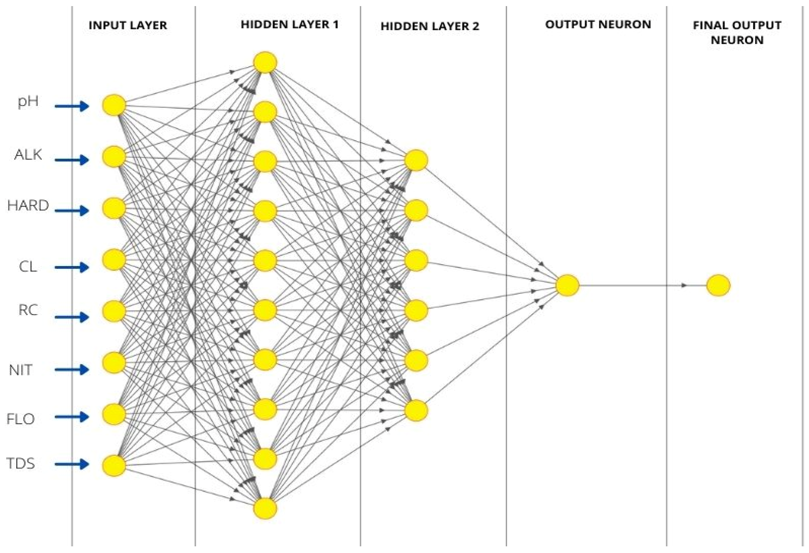
The selected neural network architecture is shown in
Figure 5. It is a four-layer network comprised of an input layer with eight nodes (each node represents one quality parameter), two hidden layers, and the final output layer with the lone node representing the quality index (WQI). The first hidden layer consists of 10 nodes connected with every node of the second hidden layer, which contains 6 nodes. The connectivity between the second hidden layer and the output layer can be seen in
Figure 5. It may be mentioned that one may use a different architecture of ANN; the number of hidden layers, number of neurons in a hidden layer, as well as the topology of the ANN structure can be varied. There are several network architecture protocols. However, an increase in the number of nodes in a hidden layer and the number of hidden layers in a classical ANN does necessarily guarantee good learning. Too much lowering of the mean square error value may lead to a situation when the ANN will learn only the pattern it is shown and will not be able to predict the outcome of a similar situation with a data set. That means the ANN may lack the capability of generalized learning. In this case, we tried to increase the number of the hidden layer from one to five with an increasing number of nodes; in the majority of the cases, the training error curve did not converge well and did not reach a low value reproducibly. Moreover, it was observed that the architecture [8]
(input)-10-6-[1]
(output) could give us a relatively better result. The training, testing, and validation curves are found to be acceptable. Moreover, one could also adopt a different technique to more authentically optimize the ANN architecture by the use of the genetic algorithm. The required objective functions of the genetic algorithm may be obtained from a preceding multivariate analysis. However, this is not within the scope of the present research. The authors propose working on artificial learning of the interrelations of water quality parameters as a separate exercise.
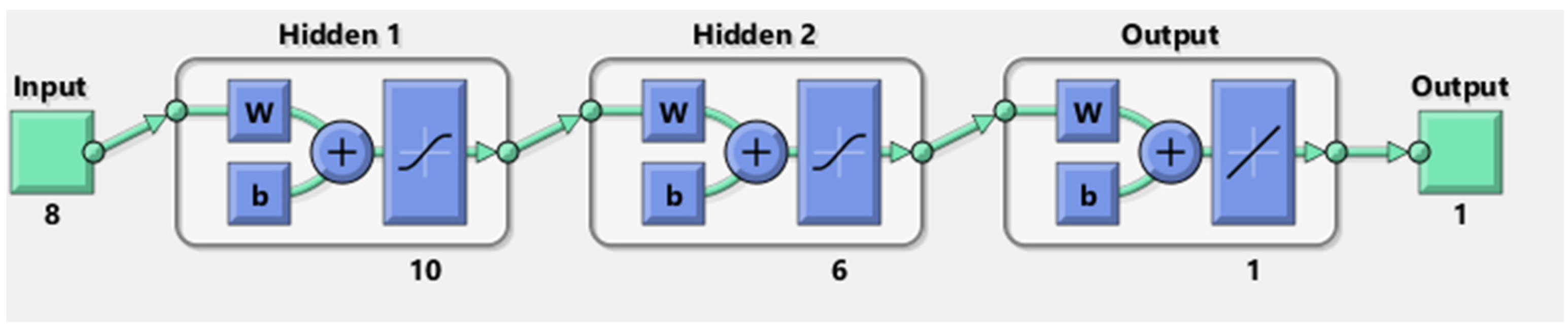
Moreover, in any such case of relational pattern recognition, it is imperative to make use of an approximator, termed a transfer function in ANNs. When we work with the related toolbox in a MATLAB platform, we have to choose any of the given transfer functions available in the toolbox. One can, of course, invoke the use of a higher-order universal approximator as a transfer function, but it would require the writing of suitable codes both for the backpropagation algorithm and for getting it interfaced with the software it works with. However, this itself will be separate research without much surety of good convergence in the problem concerned. This activity is data sensitive and hence it is an educated game to rationalize the best possible approach. The authors do not claim that the adopted strategy is the best possible one for the present data set for water quality modeling. The task pursued here is the simplest way of ensuring the predictive power of an ANN. The MATLAB platform used the feed-forward backpropagation LM algorithm to train the network. As in a classical neural network, the general scheme of data flow is also followed in the present work and is shown in
Figure 6. The data flow in the forward direction, which by the backpropagation algorithm changes the weight at each node, and the output is changed until training is stopped at a desirably low training error. It is apparent that, at each of the hidden layer nodes, the weighted input is added with a randomly chosen bias value before being put to the approximator used in the present case, which is the transfer function. The Tanh transfer function is known to be quite efficient in capturing nonlinearity [
25,
26]. In contrast, the present ANN modeling does not use any existing knowledge about the effect of the individual parameter. It has undergone supervised learning with the intent of recognizing the hidden relational pattern among the quality index assignable to the individual parameter; this kind of exercise is entirely new to its kind as there is no example where the contribution of the quality indices of eight parameters is integrated through a well-known learning process. The LM algorithm used here has produced a relatively better correlation; the authors tried with other backpropagation algorithms available in the MATLAB toolbox. The gradient descent algorithm and scaled conjugate gradient (SCG) algorithm were also tried, but in vain. We have the provision of using only those algorithms which are available in MATLAB. There is no denying that different algorithms have a different propensity for learning curves being trapped in local optima. To secure a global optimum, one needs to adopt different techniques. As stated earlier, one such technique is to use a genetic algorithm with a preceding backup of multivariate analysis. The other approach to good learning could be the neuro-fuzzy techniques; one may also test the case with unsupervised learning through the Kohonen network. All said and done, individual activity is a large task by itself and the authors have chosen the simplest one to get the idea about how the individual quality indexes interplay with one another. Apart from this, one may also prefer to use a Bayesian neural network, autoregressive moving average, or decision support system; moreover, several other deep learning techniques could also be tested for better prediction. However, for the ANN used here, the performance is best judged by MSE, R-value, and R-square and is considered to be sufficient. For other processes such as K-nearest neighbor, KNN, SVM, or the naïve Bayes model, other parameters such as accuracy, sensitivity, specificity, and F-score are used to judge the performance. Moreover, other than the use of MATLAB for the neural network, other useable software include Tflearn, Neural designer, Keras, Neuro Solution, Torch, and Microsoft Cognitive Toolkit. The neural designer can be used to mathematically model a similar data set in a code-free manner, enabling artificial intelligence (AI)-powered applications.
All 710 of the measurement data for each input variable were considered for modeling. A total of 70% of the data was taken to train the neural network, whereas 15% of the data was used for testing, and another 15% was taken for validation of the model. Since the ANN modeling was carried out in the MATLAB platform, the selection of data for training, testing, and validation was automatically random. A code was written to further randomize the given data set to reinforce the observation from the ANN modeling in MATLAB. Such random data selection was performed a number of times, and for each randomly selected data set, training, testing, and the corresponding validation were performed.
Keras can be used for purposes such as convolutional neural networks (CNNs) and recurrent neural networks. Essentially, these are deep learning software that could be used for learning the problem of the present one. The authors contemplated using the deep learning software to have better introspection into the problem being handled. The present work is a preliminary investigation to explore the feasibility of using learning techniques simulating the human brain such that one can map the relational aspects among the various parameters. It is not out of context to refer to the elegant work of Kouadri et al. [
27], where the performance of eight different machine learning techniques were used for predicting the water quality index; the artificial intelligence algorithms (AI) used by the authors were multilinear regression (MLR), support vector machine (SVM), artificial neural network (ANN), random forest (RF), random subspace (RSS) additive regression (AR), locally weighted linear regression (LWLR), and M5 P tree. While taking 12 inputs, the authors reported the superior algorithm. The authors used MATLAB for ANN and MLR, whereas for all other models, Waikato Environment for knowledge analysis (WEKA-version 3.8.4) was employed. The authors could find out the two most sensitive input parameters by sensitivity analysis, and these were further subjected to modeling, thereby observing the superiority of RF over the others; incidentally, ANN was found to be the second-best. When compared with the present work, it becomes evident that such a unique approach was used to evaluate the efficacy of ML techniques in understanding the water quality index of a particular parameter; the performance evaluation is the R-value, mean absolute error value (MAE), root mean square error value (RMSE), root-relative square error (RRSE), and relative absolute error. We contemplated a different task; after obtaining the values of quality indices of eight parameters that are considered to be a significantly important determinant of the potability of water, the unique water quality index (WQI) number for a specific geographic location is defined as per the proposed model of water quality indexing. We have been in search of a unique number that describes the water quality index in consideration of the individual parametric contribution to the overall water quality index. As has been advocated elsewhere [
27], there is a difference in the relative sensitivity of a quality parameter. It is logical to assume that the overall WQI is a complex function of the individual’s contribution (Q
i). To understand the hidden relationship, which presumes to be nonlinear, we resorted to the use of an ANN as a learning tool. Our approach is quite different from what is reported to date in respect to WQI modeling. Herein lies the novelty of our work.
Appreciating that there is a dependence of the WQI on the eight chosen water quality parameters, which assume different values for different samples drawn from different places or times, it appears to be an educated game for predicting the WQI for any set of water parameters. As a number of previous works have discussed, ANNs are one such powerful predictive tool (15–17, 21) in describing the water quality index amidst the changing water quality parameters. We have designed an ANN architecture and have performed training, testing, and validation repeatedly, each time with randomly selected data. This approach seems to be more practical than any sequential data selection strategy and is expected to avoid overoptimism. The representative performance plot of the neural network is shown in
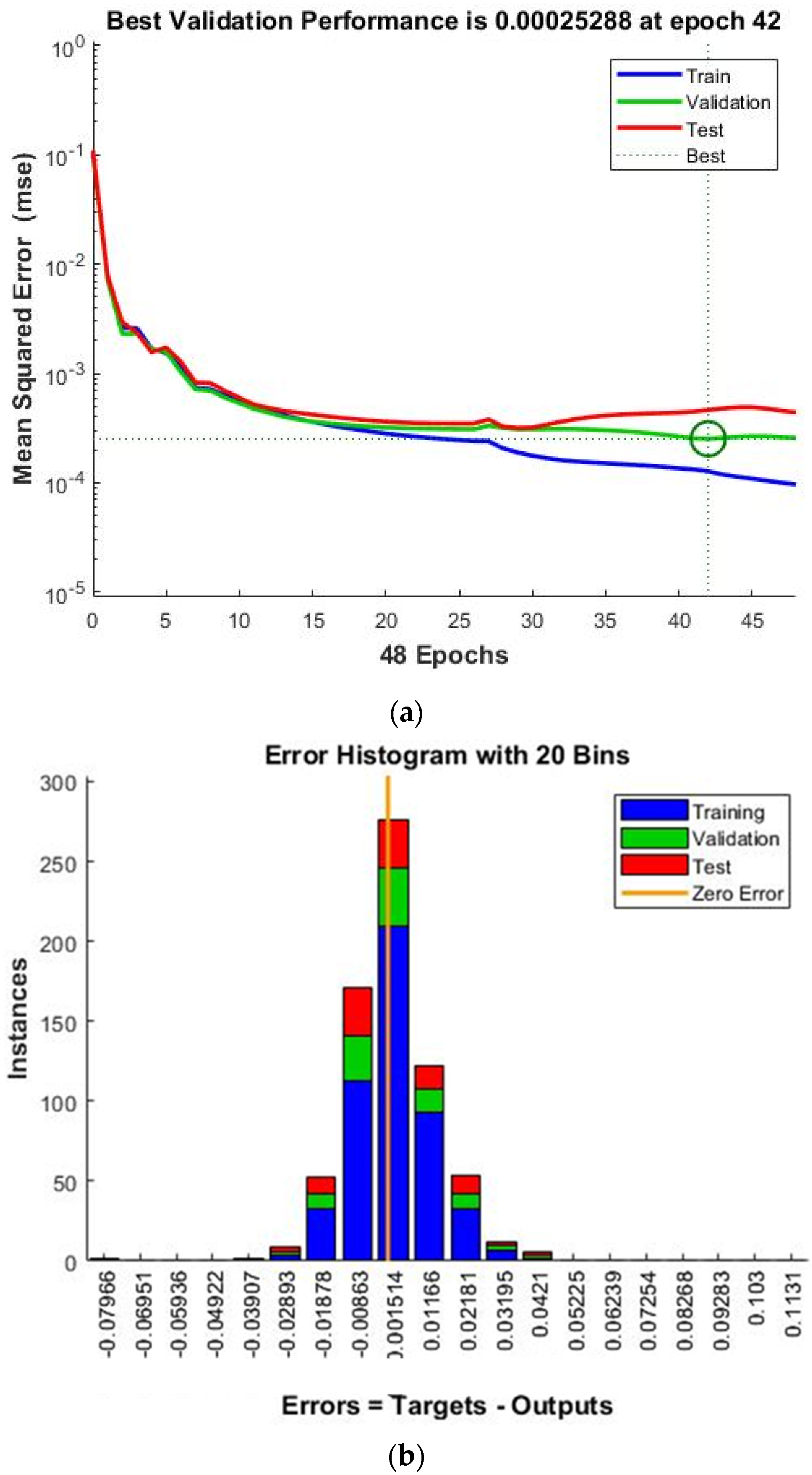
Figure 7a.
It can be observed that the training, testing, and validation error values gradually diminish, and the consistency in behavior can be noted in the figure. The validation performance is also quite good. It is evident from
Figure 7a that the test error, validation error, and training error are rather close to one another, which signifies that the designed neural network used for learning the input–output relation (WQI =
f (quality parameters)) is rather reliable. It was also found that the best achievable validation performance was 0.00025288 and was obtainable at the epoch 42. Moreover, the error histogram of training, testing, and validation is shown in
Figure 7b. It can be seen from
Figure 7b that the error defined by the difference between the target and output values is distributed over a very narrow region; this observation is valid for training, testing, and validation. It is, therefore, apparent that the present neural network is capable of effectively learning the relation between input parameters and the final output. Hence, this ANN was then subjected to further performance assessment.
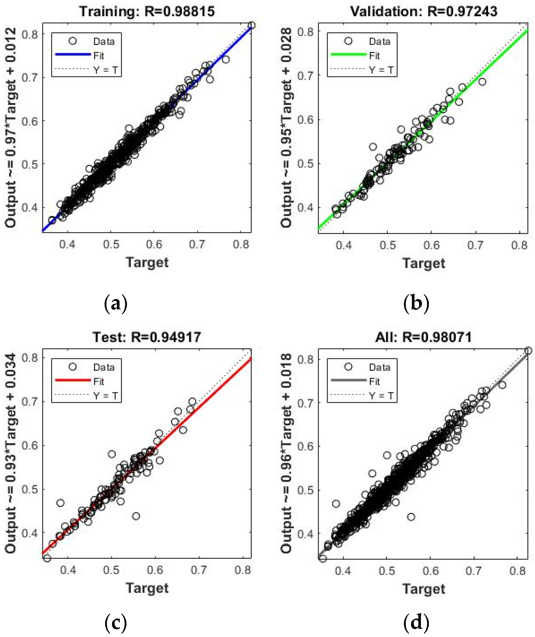
As stated in the preceding discussion, it is important to know the ability of the network to understand the relational behavior existing within the dataset, as well as the accuracy with which the ANN can predict the change in the WQI with changing values of water quality variables. The performance of the network is assessed by the correlation between the output and the target. The correlation curves obtained from the modeling in the MATLAB platform are shown in
Figure 8. It may be noted that the correlation coefficient obtained from ANN modeling in the MATLAB platform always represents the Pearson correlation coefficient.
Figure 8 shows that the R-value was 0.98815 for training, 0.94917 for testing, 0.97243 for validation, and the overall correlation coefficient, the R-value, obtainable for all the data may be as high as 0.98071. The magnitudes of the R-value for training, testing, validation, and, finally, for all data, indicate a good generalization. From the observed results in
Figure 8, it appears that the network’s performance is expectedly very satisfactory [
28].
It is known that the learning activity in a neural network involves the training of the network, during which the mean square error (MSE) is normally seen to decrease with increasing iterations. Overfitting of data may result in poor generalization; this means the network will recognize the pattern shown to it, and it will not be able to get into generalized learning. Too low an MSE value is not always desirable as it signifies that the network is trained to recognize the pattern shown to it. However, the objective is to acquire generalized learning. Hence, the network training is stopped when the desirable MSE is obtained and the performance of the network is subjected to assessment. While testing the model performance, the average value of the R2 and root mean square error (RMSE) is usually examined. As stated above, the overall model performance is quite good as one can see that the model output and the target value of the WQI bear a correlation coefficient of 0.98071, implying that the neural network has satisfactorily learned the interrelation between the input variables and the output.
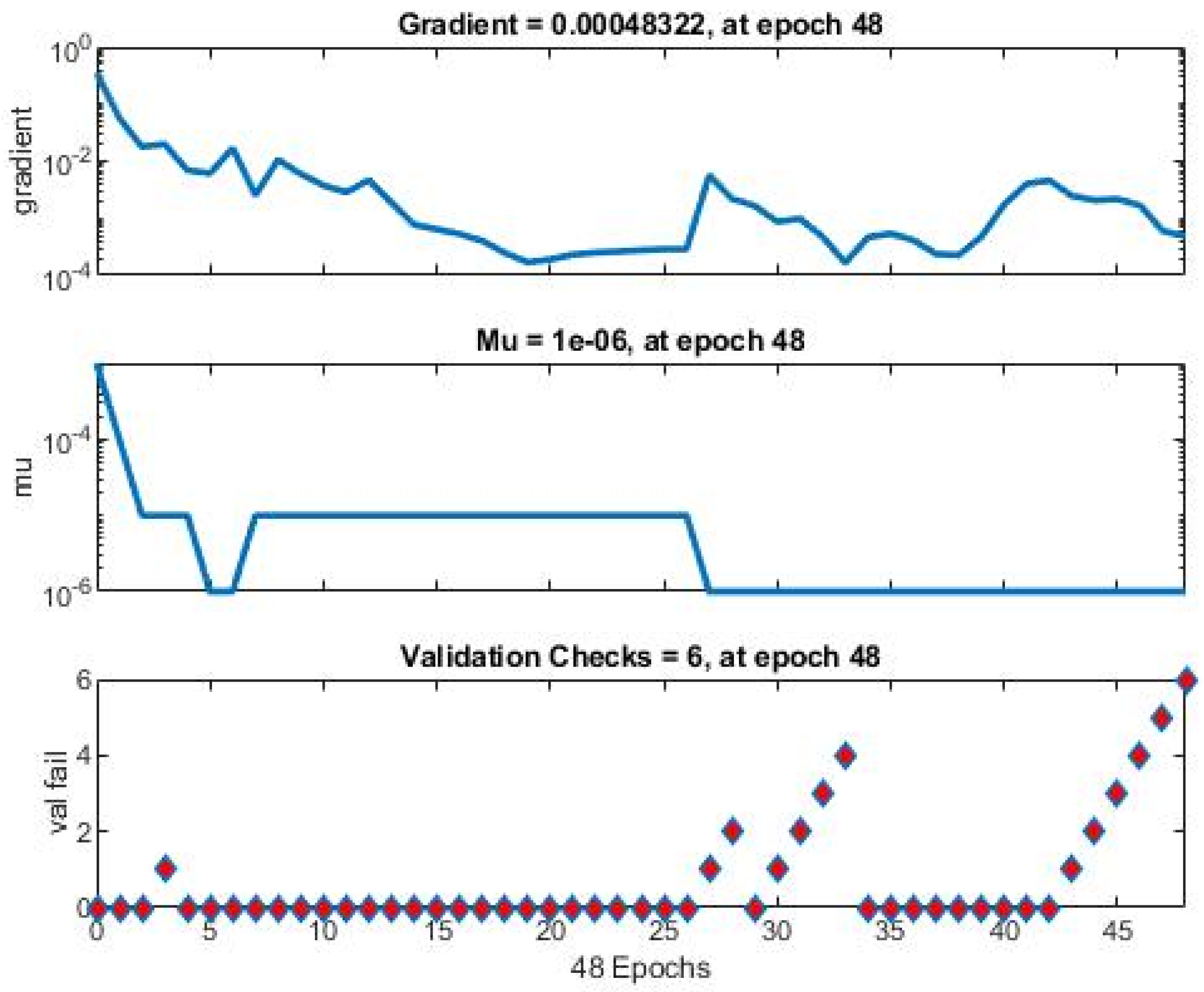
While the nearness of the R-value for training, testing, and validation indicates a good generalization, it is also essential to introspect into the training state situation to assess the overall output capability of the ANN. The training state plot for the designed network is shown in
Figure 9.
It can be noticed from the gradient coefficient that the learning rate for the learning process adopted is rather low; moreover, the validation fails against the number of epochs showing that validation checks equal 6 after 48 epochs. However, all these performance indicators of the designed ANN are presented in summarized form in
Table 3.
It can be observed from
Table 3 that the gradient coefficient of 0.00048, a learning rate of 1 × 10
−6, is achievable at a correlation coefficient value of 0.980. As stated earlier, the entire task is repeated several times with a random selection of data set at each time so that the average value can reasonably say that the model is stable. The results of ten such meaningful results are presented in
Table 4.
It can be observed that the performance parameters are quite consistent for all the ten datasets; this contributes to authenticating that the model is stable. Moreover, the performance indices of the present ANN model are compatible with similar models reported elsewhere [
17,
18,
19,
20]. It may be noted that the average value of the coefficient of multiple determination, viz., R
2 was 0.96159; the standard deviation of R
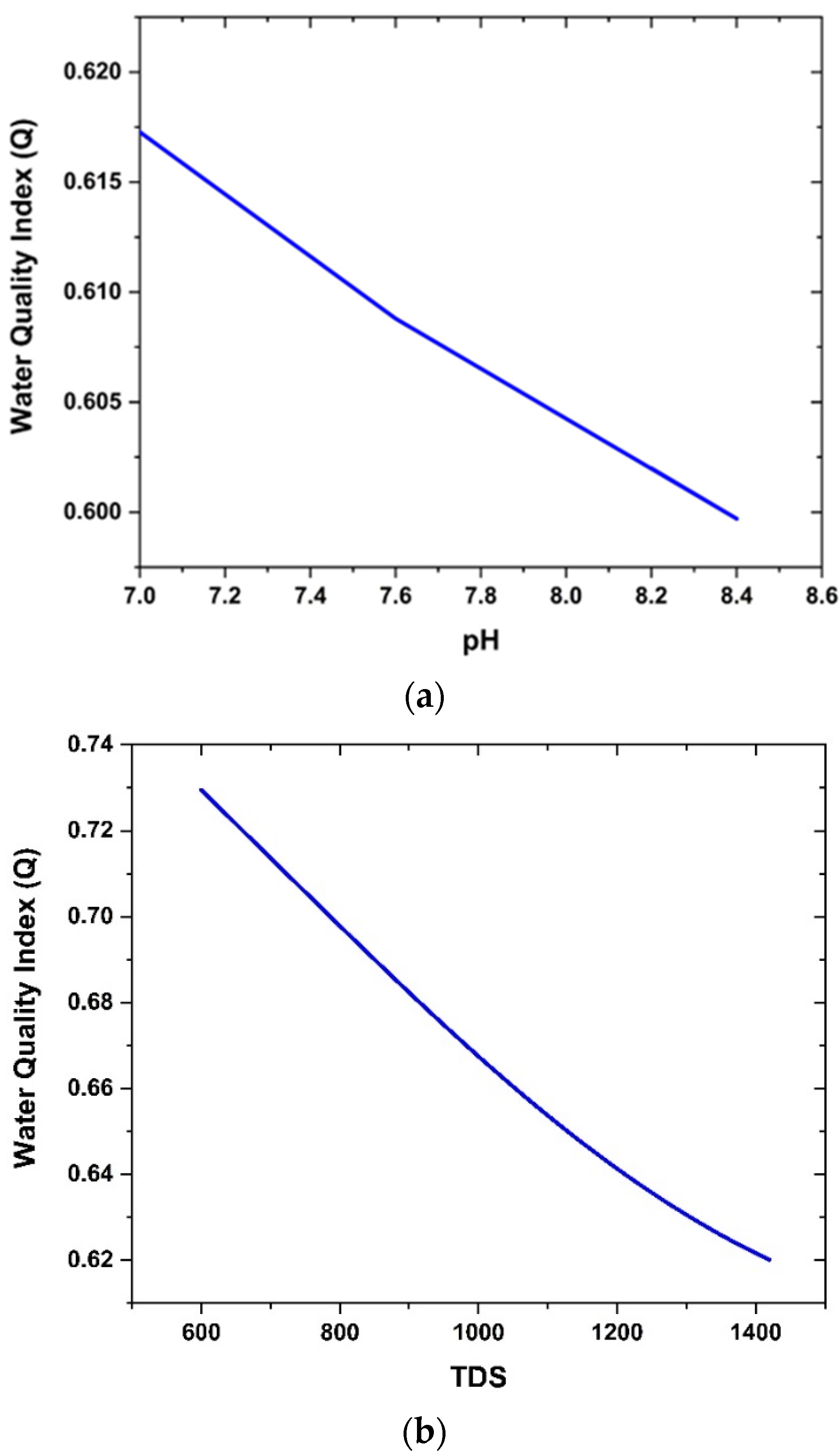
2 was also calculated and was found to be 0.00155. This authenticates the stability of the model. Generalized learning by an ANN is of extreme importance; for this reason, the predicted dependence of WQI on the input variables needs to be mapped. This is done by varying a single quality parameter at constant values of all other parameters and then finding out the WQI as the network output. Therefore, the ability for generalized learning of the ANN was verified by the results of network prediction as revealed in
Figure 10a,b.
Figure 10a shows that the network predicted the plot of variation in quality index with the pH value. It was found that increasing pH value leads to deterioration of the water quality index. This is in agreement with the existing knowledge on the effect of the pH value of water on its potability. Likewise,
Figure 10b shows how the water quality index decreases with increasing TDS. There is no denying that TDS affects the drinkability of water, and the results obtained from the use of the neural network are compatible with a well-established understanding in this regard. Therefore, it was found that the predictive capacity of the artificial neural network may be harnessed to monitor the water quality at any instant, and this finally helps in taking remedial steps to restore water quality through proper treatment.


 ,
, 


