Forensic Hydrology: A Complete Reconstruction of an Extreme Flood Event in Data-Scarce Area

Abstract

On 18 September 2020, the Karditsa prefecture of Thessaly region (Greece) experienced a catastrophic flood as a consequence of the IANOS hurricane. This intense phenomenon was characterized by rainfall records ranging from 220 mm up to 530 mm, in a time interval of 15 h. Extended public infrastructure was damaged and thousands of houses and commercial properties were flooded, while four casualties were recorded. The aim of this study was to provide forensic research on a reconstruction of the flood event in the vicinity of Karditsa city. First, we performed a statistical analysis of the rainfall. Then, we used two numerical models and observed data, either captured by satellites or mined from social media, in order to simulate the event a posteriori. Specifically, a rainfall–runoff CN-unit hydrograph model was combined with a hydrodynamic model based on 2D-shallow water equations model, through the coupling of the hydrological software HEC-HMS with the hydrodynamic software HEC-RAS. Regarding the observed data, the limited available gauged records led us to use a wide spectrum of remote sensing datasets associated with rainfall, such as NASA GPM–IMREG, and numerous videos posted on social media, such as Facebook, in order to validate the extent of the flood. The overall assessment proved that the exceedance probability of the IANOS flooding event ranged from 1:400 years in the low-lying catchments, to 1:1000 years in the upstream mountainous catchments. Moreover, a good performance for the simulated flooding extent was achieved using the numerical models and by comparing their output with the remote sensing footage provided by SENTINEL satellites images, along with the georeferenced videos posted on social media.

1. Introduction

Floods are among the most destructive natural hazards, and are caused by river overflows, flash floods of ephemeral streams, pluvial floods in the cities, floods in the coastal zone, and floods due to a potential dam or a levee failure, and with several time scales, ranging from large-scale to flash floods. Having identified a growing concern that the flood risk is increasing in Europe and globally, joint scientific efforts are necessary for establishing a reliable flood risk management framework [1]. The latter, associated with the increasing stress to the system due to urbanization and the changing climate, led the European Union to set in force the new Flood Directive 2007/60, which aims to provide a thorough investigation of the flooding risk in vulnerable areas with the use of advanced hydrological and hydrodynamic environmental approaches, and minimizing the flooding risk with structural and non-structural measures [2].

In accordance with Koutsoyiannis et al., 2012 [3], the main categories of potential flooding areas in Greece are associated with large rivers with insufficient capacity to route the natural flood and floods caused in ephemeral streams, whose cross-section dimensions have been significantly reduced by anthropogenic activities (land use change, urban sprawl). The latter, in conjunction with the limited available gauge network in the Greek catchments, offers a great challenge to the geoscience scientific community, to gather all the publicly available sources and use them within a consistent flood management framework. Flood risk management is associated with complex uncertainty sources related to hydrological, hydraulic, environmental, and social phenomena, and these sources significantly influenced the recent flooding event in Karditsa city [4].

IANOS was an intense medicane formed over the warm Mediterranean Sea. Following a path of approximately 1900 km, the medicane affected Greece, resulting in four casualties in Karditsa prefecture and devastating damage in the western and central parts of Greece. Analysis of the available observations showed that IANOS was the most intense medicane ever recorded in the Mediterranean [5]. The 15-h rainfall records ranged from 220 mm in Karditsa city up to 530 mm at the Plastiras dam rainfall gauge station. The flooding event was followed by extended public infrastructure deterioration, bridge collapses, soil sliding, and high debris flow, which were well documented by Zekkos et al., 2020 and Lolli et al., 2022 [6,7].

Several reconstructions of extreme flood events can be found in the literature, such as Borga et al. (2007) [8] and Costabile et al. (2013) [9]. Recently, similar works have been presented, providing coupled hydrological and hydraulic modelling of severe past flood events in Greece [10,11,12,13,14]. In this work, we followed the forensic hydrology framework, as proposed by Ramirez and Herrera (2016) [15], in which a reproduction of an extreme event has the following phases: (a) information gathering and integration; (b) hydrometeorological and hydrological analysis; (c) hydraulic analysis; (d) integrative analysis; and (e) final diagnosis.

According to this framework, first we used the full spectrum of available remote and gauge information to inform the spatial variability of the rainfall depths over the catchment study area. In addition, we collected observed data using new technologies, such as a remote sensing (SENTINEL platform), which indicated the flood inundation area, and crowdsourcing (videos uploaded to Facebook), which indicated the arrival time of flooding and the water depths. Then, we estimated the return period of the event and applied a rainfall–runoff hydrological model in the Kaletzis catchment (with runoffs at Karditsa city), using the HEC-HMS software, and having as an input, findings from the previous phase. The result of this phase was the derivation of the flood hydrographs that hit the greater area of Karditsa city. This is the next phase input, namely the hydraulic analysis. For this phase, a 2D hydrodynamic model was used for the flood propagation through the urban and peri-urban areas. The results of this phase were validated against the data collected during the first phase.

To our knowledge, this study is the first integrated hydrological–hydrodynamic analysis implemented for the greater area of Karditsa city, and in which a plausible check is performed regarding the results derived by numerical modelling, using a wide spectrum of satellite datasets and crowdsourced data, aiming to tackle the main challenge, which is the lack of flood-related data and measurements.

2. Materials and Methods

2.1. Study Area

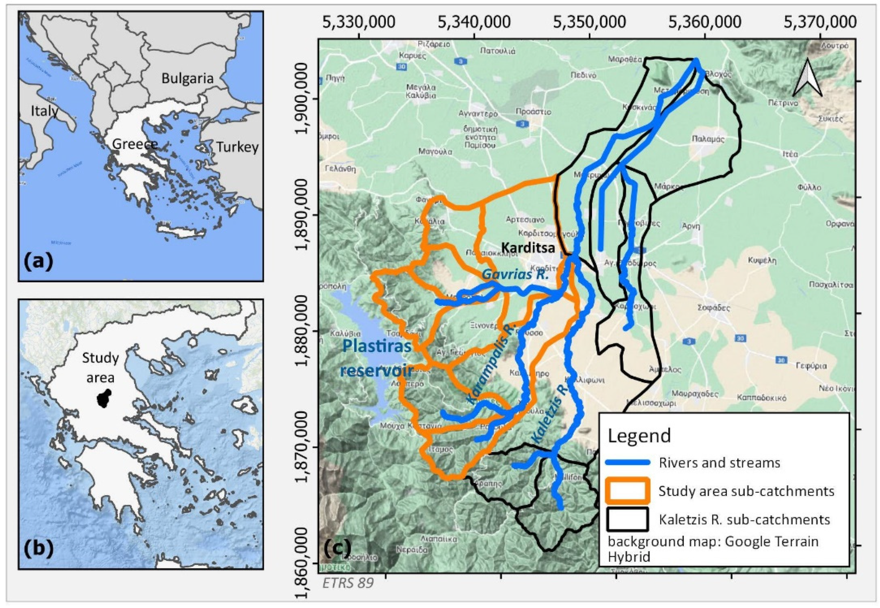
Karditsa city is located in the south-western part of the Thessaly region, Karditsa prefecture, Greece (Figure 1). It has a population of approximately 42,000 people, based on the 2011 population census. The city lies within the Kaletzis river catchment, and two rivers are drained south and east of the city, which are named Gavrias and Karampalis, respectively (Figure 1c). The Kaletzis catchment has an area of 653.8 km², while the average elevation of the watershed is 254.8 m. The maximum river length is estimated to be 66.11 km. The main sub-catchments of Kaletzis relevant to the study (marked in Figure 1c) are the (a) upstream and downstream Karampalis stream catchments, which runoff at the south-eastern part of Karditsa city; and (b) three upstream catchments of the Gavrias stream, which runoff into the south-western part of the city, and through a man-made canal are conveyed to the Karampalis river. The determination of the land cover was based on CORINE land cover data. The majority of the watershed is covered by agricultural areas and forest–mountainous areas.

On 18 September 2020, the city of Karditsa was hit by the extreme medicane IANOS. An intense rainfall that lasted approximately 15 h had as a consequence severe economic losses and damage to public assets, transportation networks, buildings, and agricultural areas, including four human losses. The city of Karditsa was flooded by extreme river overflows, mainly from the Karampalis river, and most of the urban city area remained flooded for over two days. Rainfall records from local gauges and remote sensing datasets are detailed in the forensic analysis presented herein. It should be noted that the city has a sewer stormwater gravity system, which, however, failed before the river’s flooding. Although the pluvial flood component contributed to the flooding in the city area, it was considered a small part of the fluvial flooding volume of the most intense medicane ever recorded in the Mediterranean, as the extreme precipitation magnitude recorded in the mountainous area suggests. The focus of the present work was given to the fluvial components that led to the extreme flooding of the greater Karditsa area, and the pluvial mechanism was excluded from further analysis.

2.1.1. Remote Sensing Flooding Records

The catchment area is ungauged, without the presence of flow and level gauge stations along the river system, and a reliable flood simulation is a challenging scientific task, since there are no records to validate the numerical results. Some rainfall gauges are operated by various authorities, such as the Public Power Company, National Observatory, and Minister of Public Works. In our analysis, due to the absence of a monitoring system, remote sensing dataset has been used to estimate the rainfall patterns of the IANOS event, which is in line with previous studies on event-based flood hydrological modelling [16,17,18]. Specifically, the following remote sensing rainfall has been considered for further use:

• MSWEP Multi-Source Weighted-Ensemble Precipitation
• GPM-IMREG (Global Precipitation Measurement) NASA
• CMORPH, Climate Prediction Center National Weather Service National Oceanic and Atmospheric Administration (NOAA)
• PERSIANN-CCS (Precipitation Estimation from Remotely Sensed Information using Artificial Neural Networks- CHRS Irvine)

GPEM-IMREG products and PERSIANN-CCS were selected based on record event availability.

Two re-analysis products were also collected for investigating the daily rainfall spatial extents over the catchments, namely:

• ERA5 land (ECMWF) (ERA5-Land hourly data from 1981 to present)
• MERRA land (Modern-Era Retrospective analysis for Research and Application) Global Modeling and Assimilation Office NASA.

More details on the/reliability of the remote sensing rainfall dataset for reproducing the real rainfall pattern are presented below (see Section 3.2).

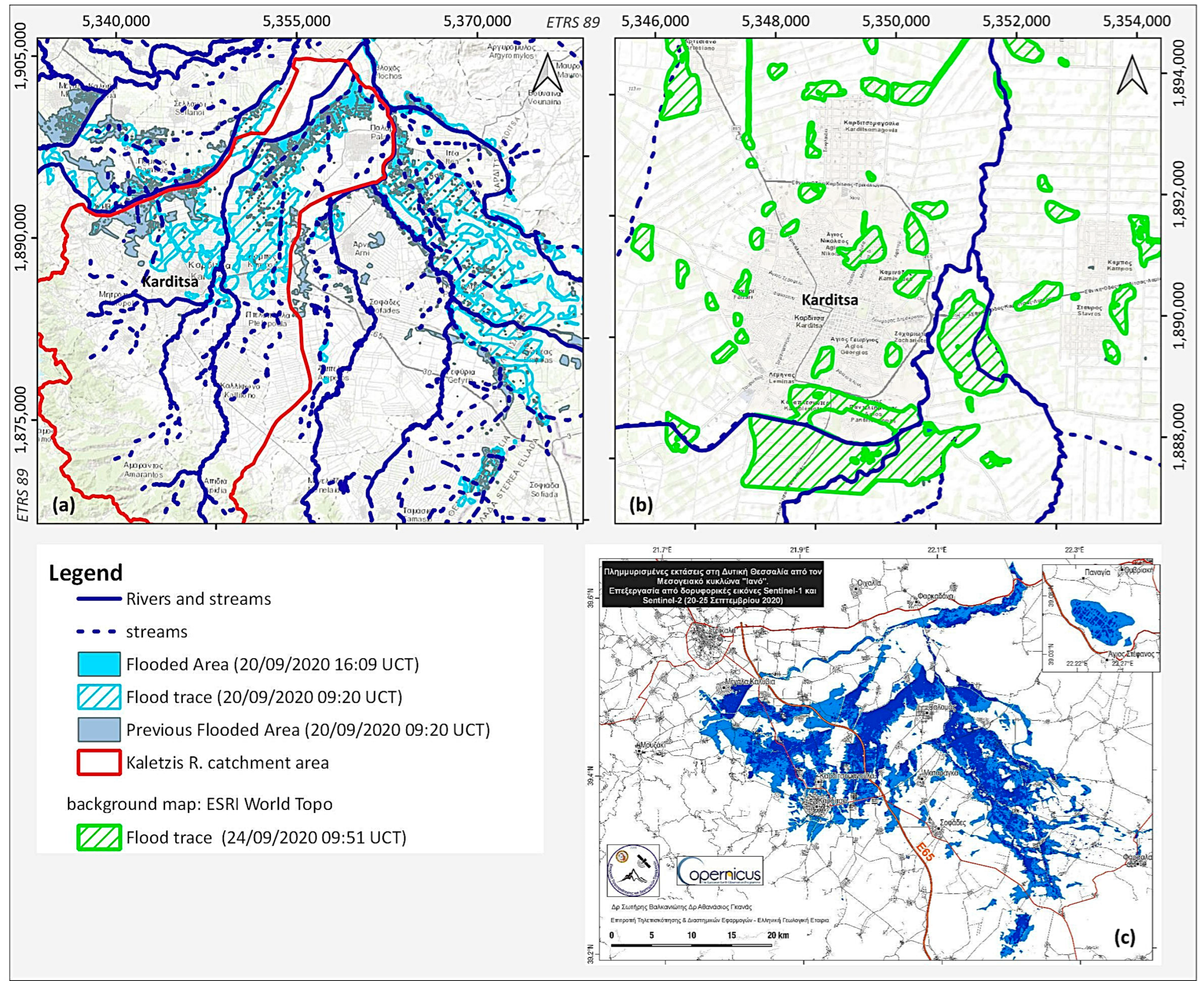
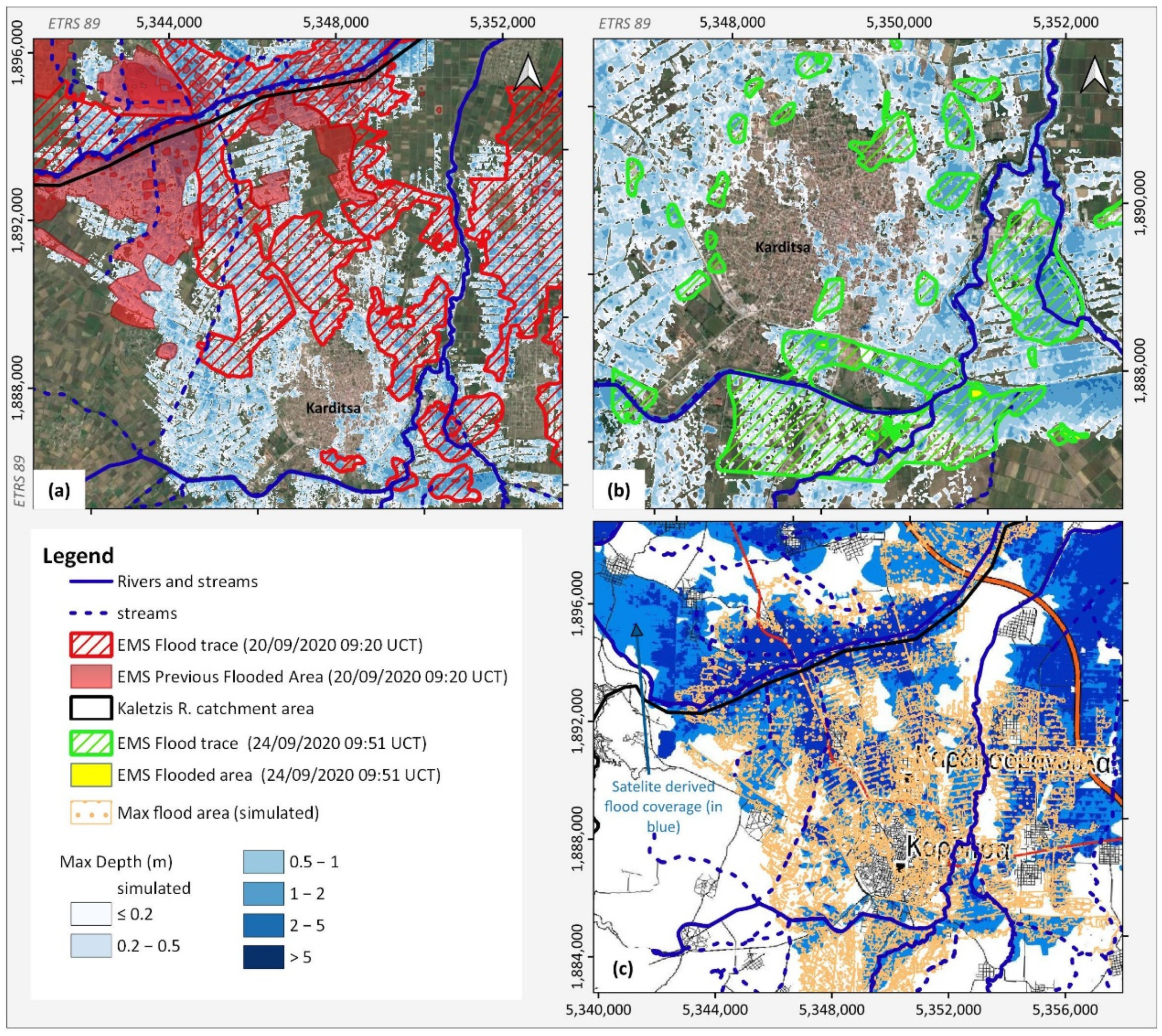
In order to investigate the flooding event and support the modeling efforts, nine flooding remote sensing recordings were collected by SENTINEL-1 and SENTINEL-2 associated with two delineation products and seven grading products, produced by the Copernicus Emergency Management Service (EMS). Remote sensing products are shown in Figure 2. Records are available for 20 September 2020 and 24 September 2020, two and five days after the main event respectively. A third post-processing map was used, and it is associated with the maximum combined flood extent captured by SENTINEL and provided by Zekkos et al., 2020 (see Figure 2c) [6].

2.1.2. Crowd Sourcing Data

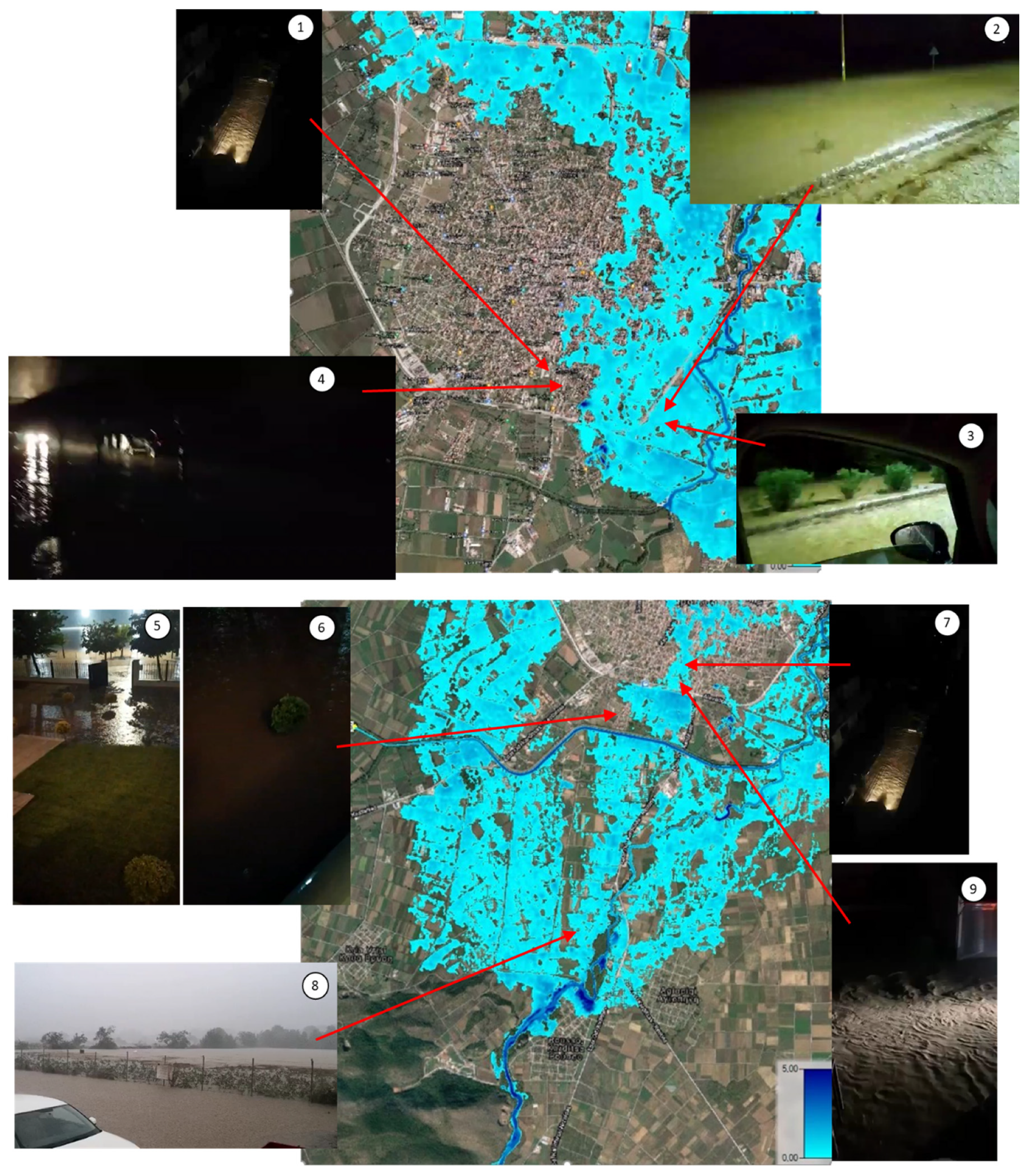
Public evidence is critical for the confirmation of a flood wave propagation [19], and therefore numerous videos posted on social media along with photos were gathered to use in the validation of the flooding extent and evolution. Nine videos were collected, which were well-distributed along the floodplain and highlight the importance of relevant information in analyzing complex flooding events. All of the aforementioned information was used in combination with Google Maps to identify (when that was possible) the location of each element-record (Figure 3). Based on the characteristics of the damage estimation records, the use of this dataset was restricted to the validation of the flood extent.

2.2. Hydrological Model Set-Up

The Hydrologic Engineering Center—Hydrologic Modelling System (HEC-HMS) software was developed by the US Army Corps of Engineers and incorporates several rainfall–runoff models, for the determination of the hydrological response of the catchments of a river. It is one of the foremost and most globally well-known software tools for the hydrological simulation of flood relief schemes, drainage, flood early warning systems, dam design, debris flows simulation, etc. [13,20,21]. The Kalentzis catchment was delineated and divided into 16 sub-basins using the HEC-GeoHMS extension in ArcGIS. Terrain preprocessing and basin processing tools were used to generate the basin model file containing the drainage network and delineated catchment. Precipitation was estimated using the Thiessen polygon method and suitable weights for each subbasin were defined to create a meteorological model. Remote sensing rainfall datasets and gauged rainfall records were compared to identify the most suitable rainfall pattern. More details on the aforementioned comparison are provided below. As an outcome, gauged precipitation data from the Karditsa (sub-hourly) and the Plastiras dam (15-min) gauging station were selected.

In general, HEC-HMS allows for the separate modelling of hydrological processes; loss, transformation, baseflow, and routing, with several models for each process. The selection of the model for each process should be based on the catchment characteristics, data availability, and whether the simulation is event-based or continuous. The SCS-CN unit hydrograph method was selected to simulate the transformation, in conjunction with the deficit and constant loss method, and the recession baseflow model. The lag time t_p, which is a parameter required by the methodology, was defined as the time period between the centroid of excess rainfall and the peak discharge. The later was calculated for each sub-basin using the Giandiotti equation [22], in order to derive the time of concentration. Average soil-moisture condition was selected considering the active irrigation period for the extended irrigation areas in low-lying catchment areas, and a small rainfall of about 10 mm occurred before the main flooding event.

Regarding the routing method, the well-known Muskingum–Cunge model was applied to all reaches, with a Manning n coefficient equal to 0.040. Parameters such as reach length and slope were estimated using topographical data. The overall hydrological schematization follows the technical specification of the Flood Directive implementation in Greece, and more details are provided by Papaioannou et al. [23].

2.3. Hydrodynamic Model Set-Up

The HEC-RAS software was used for the hydraulic routing simulation of the flood hydrograph through the Karditsa town stream network. It is a well-known software developed by the Hydrologic Engineering Center (HEC) of the U.S Army Corps of Engineers and used for river flood modelling and floodplain management [4,11]. Since the data availability was limited (lack of detailed river surveys, extended low-lying flood plains) and as the urban and peri-urban area of Karditsa city is quite complex, having multiple hydraulic directions due to a low-lying surface, we selected the two-dimensional (2D) mode of the HEC-RAS software. The latter mode is either based on the full form of the 2D shallow water equations (2D-SWE) or in 2D diffusion wave equations, which were selected after a sensitivity analysis, with respect to numerical accuracy and computational time. The latter approach was successfully applied in similar projects in the past, especially in data-scarce areas [11,13,24]. It should be mentioned that the hydrodynamic model setup was developed in line with the Flood Directive contracts, as previously outlined by Papaioannou et al. [23].

The importance of DEM accuracy has been highlighted by several authors, especially in two-dimensional hydraulic–hydrodynamic modelling applications [25,26,27]. To meet these requirements, a DEM with a horizontal resolution of 5 × 5 m generated from aerial images collected from 2007 to 2009 and provided by the National Cadastre and Mapping Agency S.A. (NCMA) was used in this study.

A critical parameter in hydrodynamic modelling applications is the selection of the roughness coefficient in the entire computational area [28]. In this work, we coupled the corresponding values proposed in Greek Flood Management Plans [29] informed by LAND COVER maps.

One of the modelling challenges was the representation of various hydraulic structures, such as bridges, culverts, weirs, etc., with respect to the cell size and their false description within the DEM. A non-detailed DEM spatial resolution, in combination with the appearance of natural or artificial structures close to the flood mitigation works and hydraulic structures, can lead to distortions of the elevation and by extension to their false representation within the DEM. To overcome this problem, a sensitivity analysis was carried out at the locations where structures exist. In order to represent the structure’s roughness and potential blockage effect during the flood event, a local increase of the Manning coefficient was justified. A sensitivity analysis was also carried out, regarding the optimal computational grid size, which influences the modelling accuracy [27] and the computational time substantially. Based on this analysis, we selected a squared grid-size of 20 m.

3. Results

3.1. Extreme Statistical Analysis of Plastiras Reservoir Annual Runoff

As previously described, there is lack of long-term reliable gauge records in the riverine system, which would offer the capability to understand the complex transformation from rainfall to real runoff. To overcome this problem and in order to assess the exceedance probability of the IANOS flooding event, an annual extreme statistical analysis was carried out for 12-years of the annual max daily water level of the Plastiras reservoir located in the west of the study area. The reservoir is a multipurpose reservoir operating for 70-years and having irrigation, water supply, and tourism uses [30,31]. HYDROGNOMON software was used to fit numerous suitable statistical distributions [32].

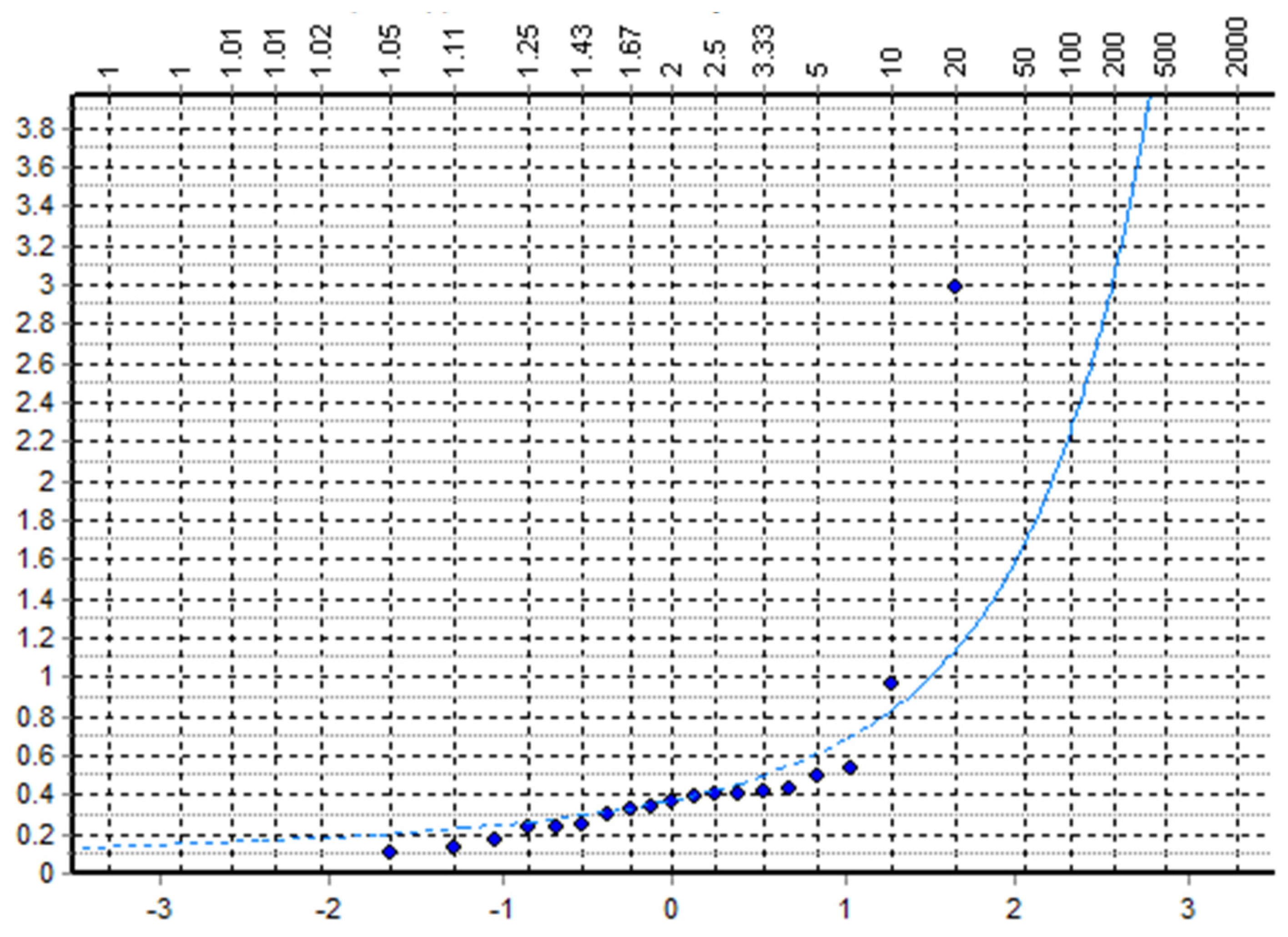
EV2-max was selected as an appropriate statistical distribution, after applying the Kolmogorov–Smirnov test. Figure 4 visualizes that the daily 3-m reservoir level rise approximately corresponds to a 1-in-200-year event (according to the theoretical distribution). The statistical analysis is shown herein only for indicative purposes, since the 12-year time record was insufficient for demonstrating a reliable extreme statistical analysis.

3.2. Rainfall–Runoff Analysis

A comparative analysis was performed for the spatial variability of the rainfall regime, using a suite of the available remote sensing dataset rainfall records and rainfall gauge records at fine time scale. For the hydrometeorological formation of the extreme phenomenon, the readers are encouraged to study the work presented by Karagiannidis et al., 2021 [5].

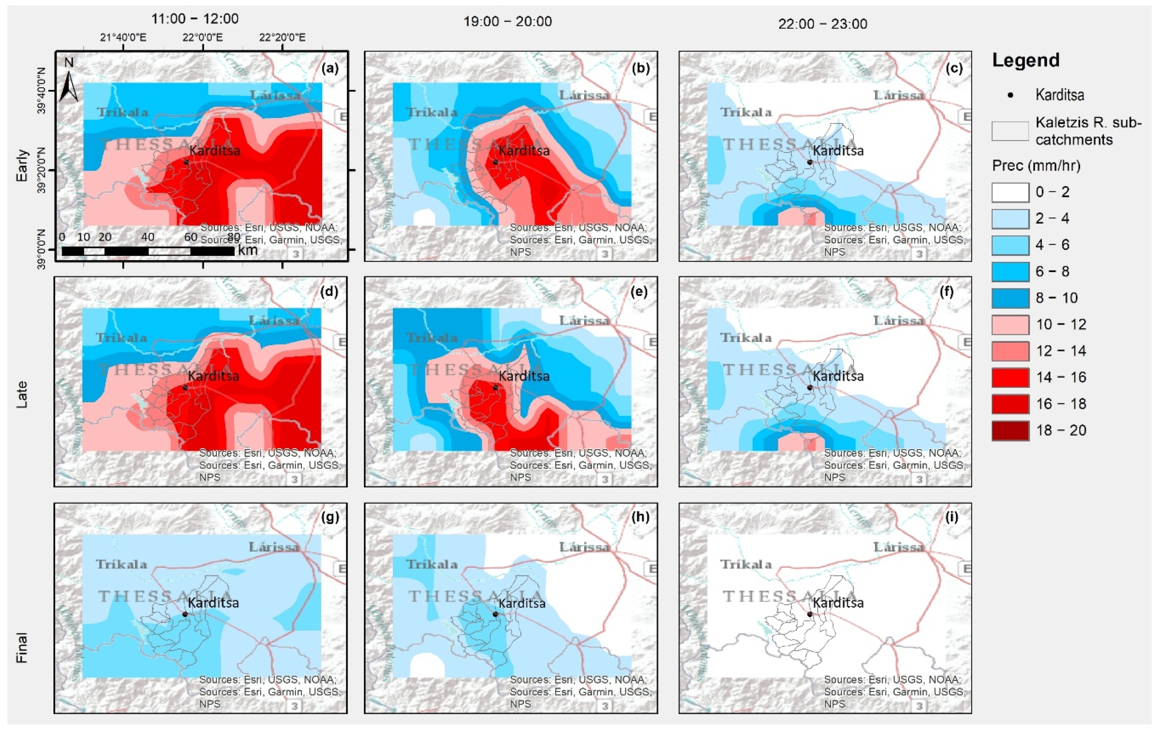
As outlined above, three NASA GPM–IMREG products were assessed, named according to the initial assessment of the satellite records, and specifically the “Early”, the “Late”, and the “Final” products, which include further post-processing based on the ground meteorological observations. The “Final” product has significant differences in comparison with the corresponding “Early” and “Late” versions, due to the use of a climate change adjustment factor. It significantly underestimates the magnitude of the precipitation and presents a “buffered” and smooth temporal distribution, contrary to the data captured by local, ground measurements. Therefore, it fails to reproduce the IANOS rainfall spatial event. It seems that the “Late” product is the most suitable for describing the spatial variability of the extreme meteorological event, since it presents a better fit for the ground measurements of the representative ground stations for the study area, in terms of total precipitation, as well as the temporal distribution of precipitation. Figure 5 depicts the NASA satellite products for different time records. The higher rainfall records in the vicinity of the study area for both Early and Late products can be seen.

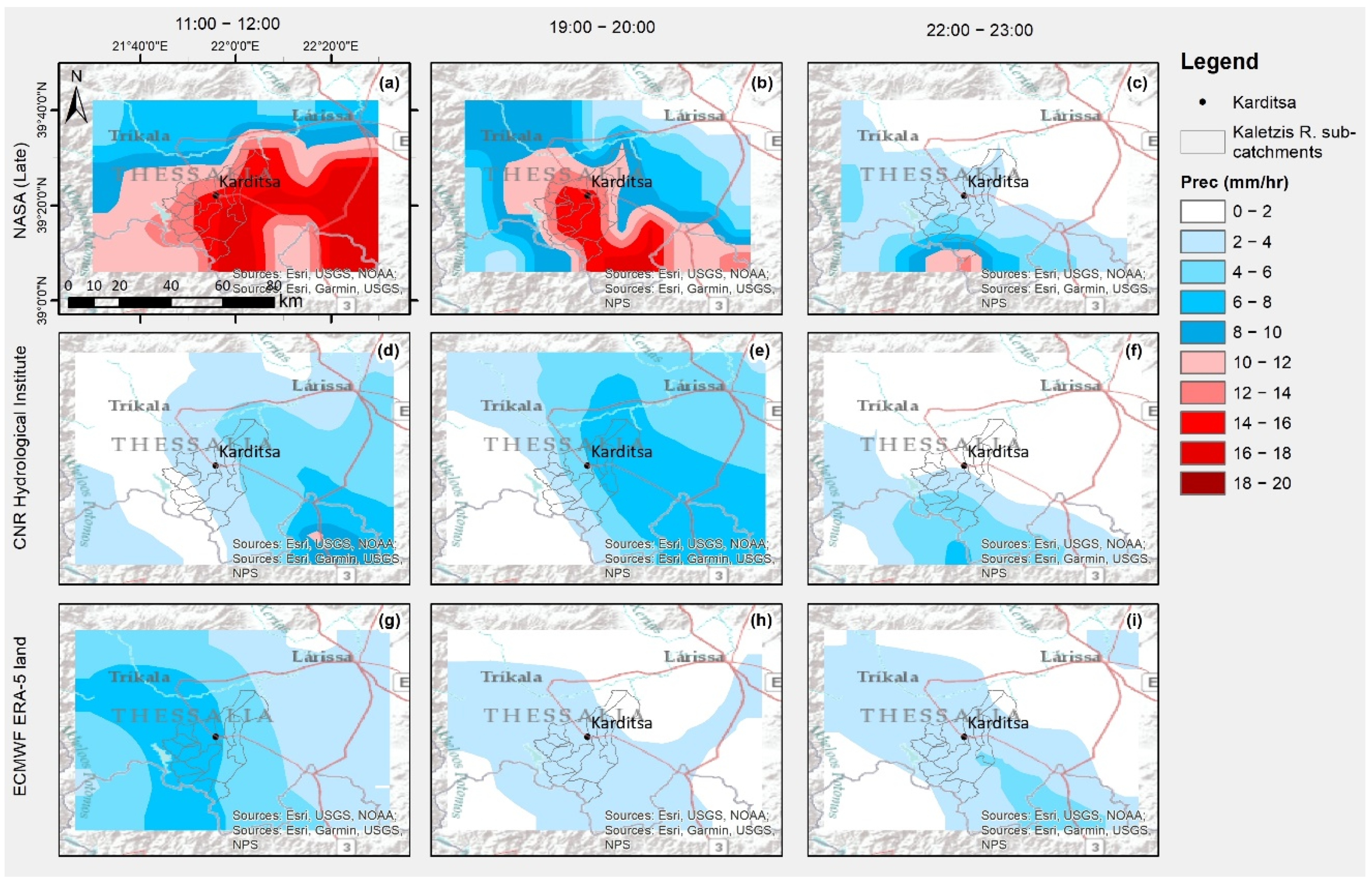
Except for the above, two reanalysis remote sensing products were also gathered and analyzed in conjunction with three NASA GPM–IMREG estimates: the ERA5 land-CNR and the MERRA land-NASA reanalysis products. Both of them underestimate the rainfall in comparison with the NASA-GPM–IMREG, as observed in Figure 6.

Following on from the above comparative analysis, it can be concluded that NASA’s and CNR’s remote products show better agreements and greater rainfall depths in the south and southeast of the study area. In contrast, ERA5 land (ECMWF) shows higher rainfall depths in the southwest of the study area. Figure 7 exhibits the daily cumulative rainfall depths retrieved by the aforementioned remote sensing products. The NASA GPM–IMREG Late product shows a higher daily rainfall depth of up to 200 mm and a better performance for the greater area of the city of Karditsa. ERA-5 and CNR products present substantially lower records, of up to 100 mm.

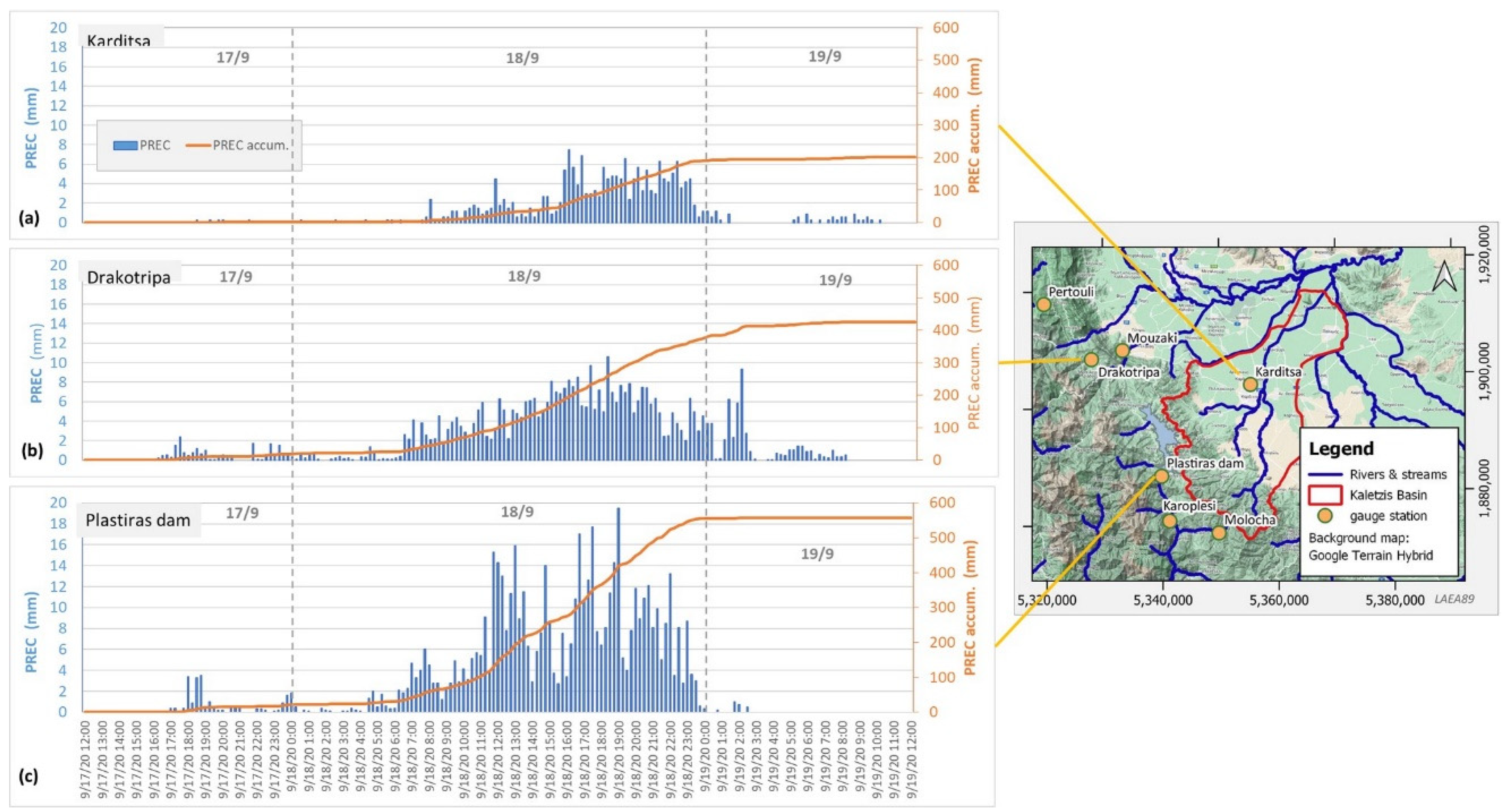
All the remote sensing products failed to provide accurate rainfall records in comparison with the gauged rainfall records. Specifically, the 15-min records from the Plastiras dam gauge station west of the study area exhibit a relatively higher record of approximately 530 mm in the 15-h time period on the 18 September 2020. Karditsa’s rainfall gauge station provides a lower record of 220 mm for the same record period (Figure 8).

Although the remote sensing precipitation products underestimated the magnitude and intensity of the phenomenon, they provided useful insights regarding the evolution and spatial variation of the phenomenon. The spatial information revealed, indicates that the available gauging stations captured the spatial variability of the event’s precipitation and could be used for the hydrological investigation. In the light of the above analysis, the gauge rainfall records were the most suitable for the flooding event analysis; and following a Thiessen analysis, the point records of Plastiras dam station and Karditsas station were mapped over the sub-catchment of the study area. The mountainous sub-catchments have a significantly higher rainfall input, influenced by the Plastiras dam record representing 30% of the total catchment study area. The low-lying catchments were impacted by Karditsa’s station rainfall record.

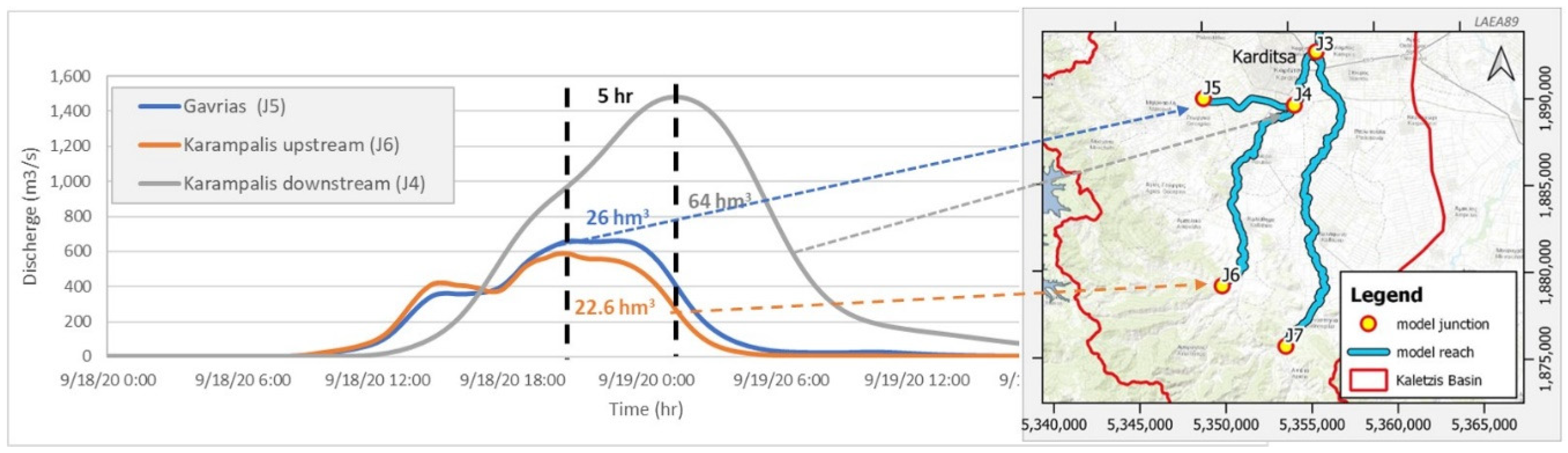
The final output of the HEC-HMS software is depicted in Figure 9. Specifically, three flood hydrographs are presented at the junctions of interest. For the J5 junction of the Gavrias river (which is located in the southwest part of the city), the maximum peak flow was simulated as about 630 m³/s, while the time to peak was estimated as about 12 h. The Karampalis upstream junction J6 peak flow was estimated as about 600 m³/s, while Karampalis downstream junction peak flow was estimated as about 1400 m³/s. At the latter junction, the Gavrias river and upstream Karampalis are connected. The latter provided a specific event discharge ranging from 5.06 to 10.5 m³/s*km². It is worth mentioning that the time to flooding responses of the Gavrias and upstream Karampalis sub-catchments coincided, leading to a very high peak flow in the east part of the city.

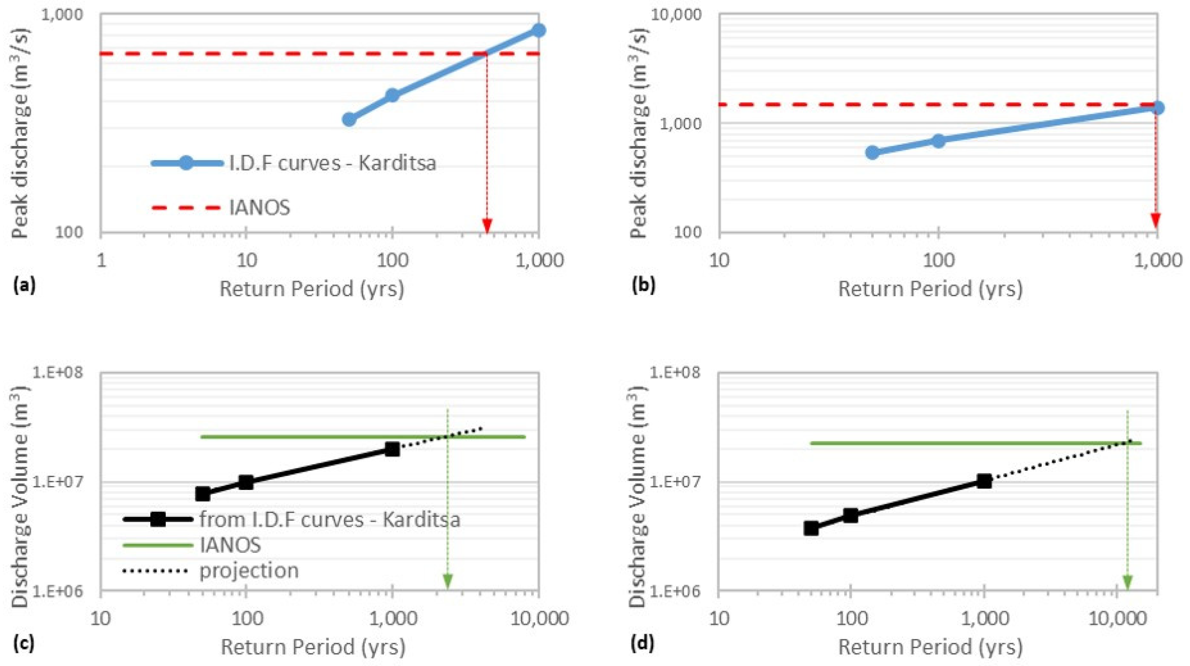
In order to quantify the return period of the IANOS event, three rainfall scenarios were developed using the intensity–duration–frequency curves of Karditsa station, namely T = 50 years, 100 years, and 1000 years. The latter was developed as part of the national implementation of the Flood European Directive [33]. A recent framework presents more insights into the regional implementation of the intensity–duration–frequency in the study area [34], and it is recommended for defining the extreme rainfall depths for different exceedance probabilities.

Figure 10 shows the plots of the estimated return period with respect to the flows (a and b), as well the flooding volumes (c and d), which are the equivalent volumes extracted by the flow event hydrographs. It was calculated that the IANOS flooding event’s return period is around 400 years for the downstream low-lying catchments and about 1000 years for the upstream mountainous catchments. Most interestingly, the flooding volume return periods were estimated as being 1000 years for the low-lying areas, and for the upstream catchments reaching 10,000 years, highlighting the catastrophic nature of the flooding event.

3.3. Flood Mapping

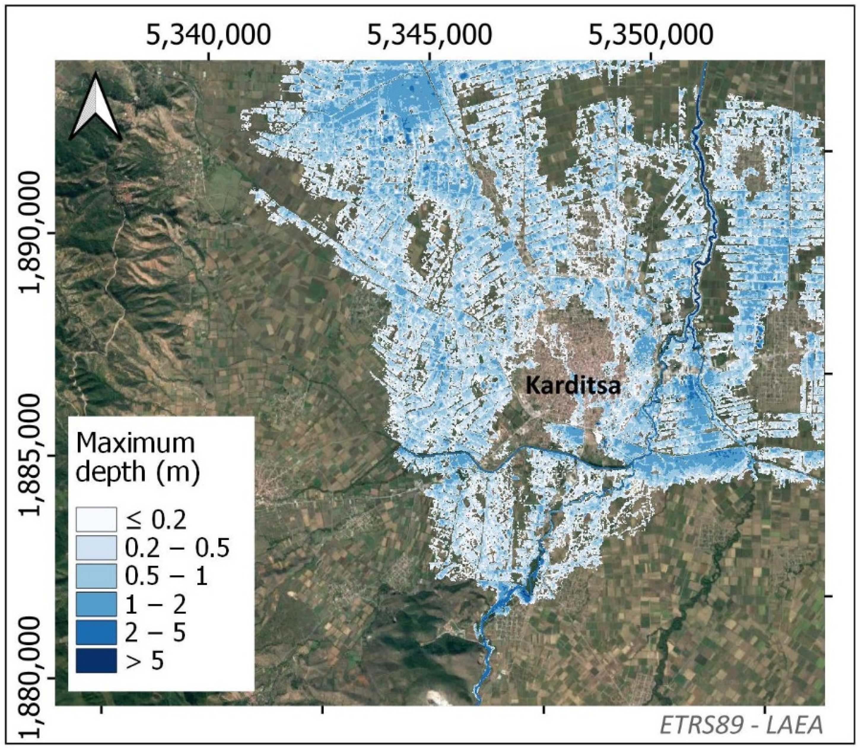
Figure 11 presents the maximum water depths and the maximum flood extent simulated by the HEC-RAS software, having as an input the HEC-HMS output for each junction point, namely J4, J5, and J6. An extensive overflow of the upstream Karampalis river was observed in the south part of the city areas. The Garvias river was flooded in the northwest part of the city. Its overflow was directed to the north, while the remaining flows were routed through the man-made canal in the north part of the town as well. It is worth mentioning that the extreme flows from the upstream Karampalis catchments had as a consequence the overtopping of the Gavrias river and the railway rail embankments. These overflows were propagated from the north floodplains to the city center through the complex urban stream network. The most severe overflows that impacted the city were observed in the east Karampalis river, downstream of the junction with the Gavrias river.

For the main channel of the river, the maximum water depth was simulated as about 5 m, while the corresponding maximum water depth in floodplain was about 1 m. All the simulations demonstrated that the city was hit by a significant flooding wave coming from the west, east, and north.

3.4. Validation

Since remote flooding footage is critical for validating the performance of our simulations, three satellite flooding footages were used to compare the simulated flood extent with the observed flood extend [35]. In this vein, two SENTINEL satellites images were acquired from the Copernicus EMS service: (a) the first refers to approximately 35 h (date 20 September 2020) after the estimated peak flow of the flood event; (b) the second refers to the flooding extent 5 days after the event. In addition to this dataset, a post-event flood image was acquired by Zekkos et al., 2020 [6] and is also presented here. Post-event satellite images of the same day or the next day after the flood were sought, in order to supplement the analysis with an as recent as possible flood extent delineation. However, the cloud coverage was dense for these dates, significantly reducing the potential of those images for useful flood extent delineation.

Figure 12 shows the simulated flood extent, in comparison to the observed flood extent provided by the satellites. The performance, in terms of the main flooding extent and the capturing of the main, overland flood pathways, was satisfactory. As expected, the simulated flood extent was greater than the three observed extents. The observed footage is a snapshot, referring to significantly later observation times, varying from 1.5 to 5 days post-event; while the simulated flood represents the maximum flood extent during the development of the phenomenon. It can be safely assumed that, in the period following the flood, the overflows were drained through the town’s sewer network.

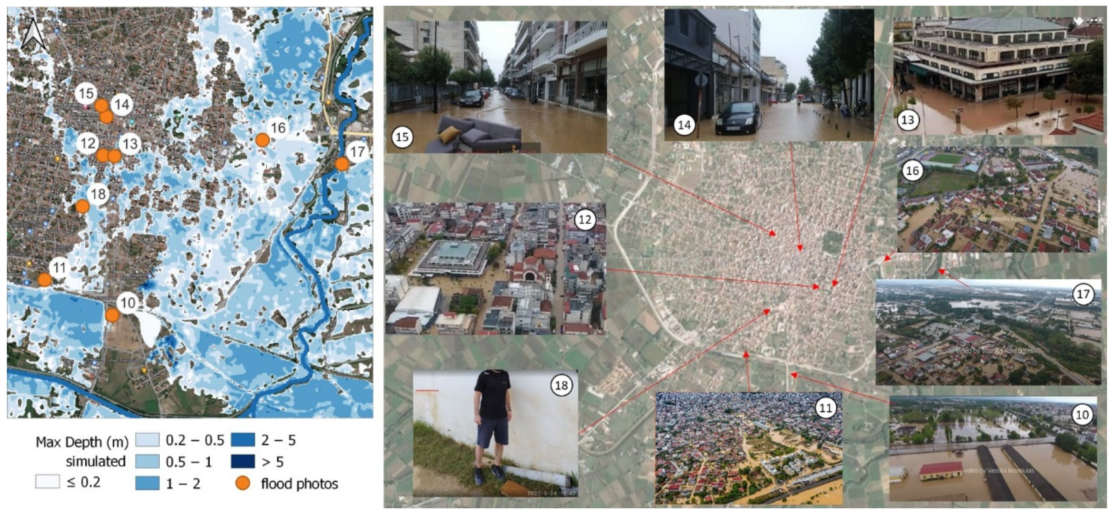
In addition to the remote sensing data, crowdsourced photos and videos captured by social media were used, in order to perform a plausible check of the simulated flood maps and evolution of the simulated flood. Numerous georeferenced photos were posted on Facebook approximately 12 h after the peak flow. Some of these are depicted in Figure 13. Furthermore, several posted videos exist, which are provided in the appendix. As mentioned in the previous section, the town’s sewer system was submerged during and after the flood event. As the gauging records reveal, extreme precipitation was recorded in the mountainous part of the basin. Although the pluvial flooding component contributed to the flooding in the city area, it was considered a small part of the fluvial flooding volumes. Therefore, we focused our analysis on the fluvial flood component, coming from the Gavrias, upstream Karampalis, and downstream Karampalis rivers.

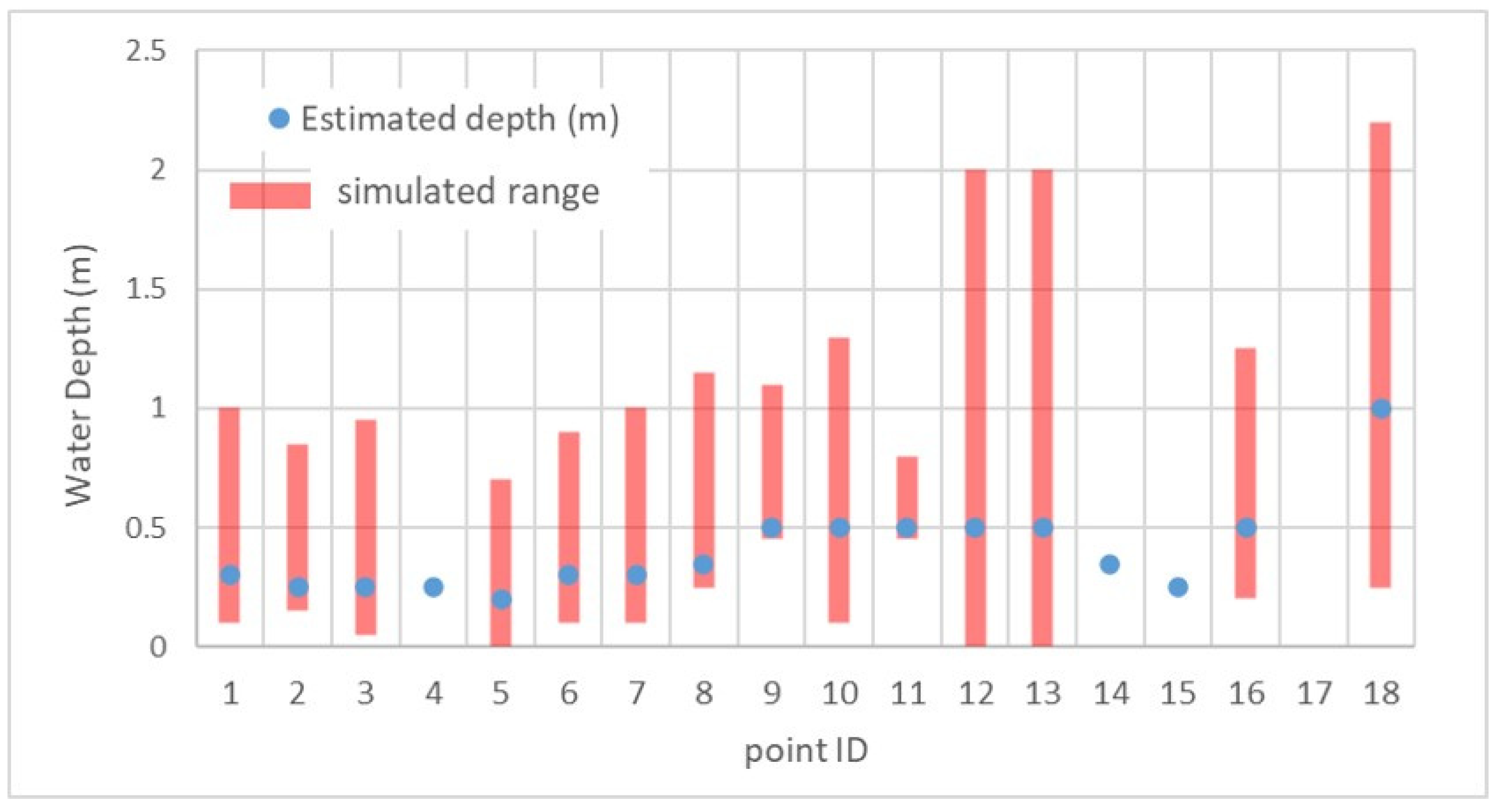
Flood depth estimations were made based on the crowdsourced data. Two sets of estimations were carried out. Photos of the next day (19 September 2020, see Figure 13) were utilized to estimate the depth that the flood reached (positions 10 to 18). These depths were compared with the maximum simulated depth in those positions. Furthermore, videos capturing the evolution of the flood were utilized to estimate the depth at the time of the video capture (see Figure 3, points 1 to 9). The depth estimation was conducted based on expert judgment and knowledge of the area. In order to validate the model, the simulated flood depth was calculated for the corresponding observation points (1 to 18). Due to the uncertainty of the depth estimations based on the photos and videos, as well as the fact that the areas captured in the photos do not represent a single, specific point, the corresponding modelling depth was calculated for an area of 1 cell radius (when larger areas were depicted in photos, larger areas were used from the model results), as a range of values. The range of the simulated depth values was compared to the estimated ones in Figure 14.

Based on this comparison, the estimated observed values lie within the range of the simulated depths. The modelled (averages) depths overestimated the estimated actual depths by about 0.25 m or less in the majority of positions considered. Additionally, the spatial (between observation) variation of the estimated observed values is consistent with the variation of the corresponding modelled (averages) depths. Based on the above, and taking into account the various factors of uncertainty, the agreement between modelled and observed values is considered satisfactory.

4. Discussion

Herein, we discuss how our analysis can contribute to existing knowledge, in order to reconstruct past flooding events using a suite of remote sensing datasets, limited gauged records, rainfall-runoff modelling, and 2D-hydrodynamic modelling. The main findings and issues for further consideration are presented below:

• Both the rainfall spatial and temporal variability is of high importance in order to reconstruct a past flood event with reliability, especially in small catchments with high complexity (Bellos et al., 2020 [10]). Topography in smaller scales (such as local horographic phenomena) is a factor that can significantly affect the meteorological conditions of the atmosphere. For this reason, the scientific community has turned its attention to meteorological satellite and meteorological radar products, in order to derive distributed rainfall data, both in space and time. However, in our study the remote sensing rainfall dataset at fine time scale (namely 30 min records) seemed to underestimate the order of magnitude of the storm, in comparison with the ground meteorological stations. This is probably due to the fact that the space step of the satellite product is rather large and smoothens the extreme rainfall intensity, which was (fortunately) captured by the ground observations. Needless to say, this is not a global conclusion, but an ad hoc remark based on our study. In the end, there are no doctrines for reconstructing a flood event: all the available rainfall products should be evaluated and used.
• The latter agrees with the recent global analysis presented by Pradhan et al., 2022 [36], an analysis of an extreme event in Mexico [37], highlighting the requirement for further improvements to achieve a higher rainfall estimate accuracy [38]. Similar results were presented by a comparative evaluation of GPM IMERG Early, Late, and Final hourly precipitation products over the Sichuan Basin, China [39]. Most interestingly, our findings, where the Early-run product was found to have a better performance than the Late and Final IMERG products, agrees with recent research on the Evaluation of IMERG GPM products during Tropical Storm Imelda [40]. An additional source of rainfall data is also the meteorological radars, which can achieve a better accuracy and denser resolution for both space and time. Finally, the importance of expansion of the ground meteorological network should not be underestimated. In the end, ground observations are the only “reality”, compared with the proxy data provided by satellite and radar products.
• Integrated catchment modelling is the most significant tool for reconstructing a past flood event. In our case study, we linked a rainfall–runoff model with a 2D hydrodynamic model and compared the model output with crowdsourced data. Regarding rainfall–runoff modelling, caution should be taken when assessing the time of concentration of different sub-catchments and assuming the pre soil moisture conditions of the catchment. All these parameters are very sensitive for reliable flow estimates in ungauged catchments and have already been referred to in previous studies [41,42,43].
• The question raised by Apel et al., 2009 [44] is still valid, in respect to how detailed we need to be in flood modelling. In our case, the 2D hydrodynamic modelling of an extended low-lying irrigated area exhibited a satisfactory performance in reproducing an extreme event; however, 2D-modelling has some shortcomings (e.g., of blockage bridge assessment under high debris rates). It is recommended that the modelling analysis should be always considered in conjunction with the available survey information, as well datasets for validation. We should highlight that we cannot exclude a priori any modelling option (2D or full 1D hydrodynamic modelling) and this is subject of the data availability in each case study.
• Our analysis introduced a data-driven integrated hydrological–hydrodynamic assessment of a major past fluvial event, including several datasets for validating our model approaches. It was based on a deterministic approach, which is the current practice for natural hazards and exhibited satisfactory results herein. However, given the complexity and uncertainty associated with the hydrological and hydrodynamic components, probabilistic flood mapping approaches [2,4], coupled hydrological–hydrodynamic physically-based numerical modelling [45], and the recent hybrid-stochastic approaches are strongly recommended [46], especially when we deal with real-world engineering design.
• It is generally accepted that flood studies suffer from a lack of data. The majority of the basins are ungauged, and in gauged basins an extreme and violent event, such as a flood, can destroy the monitoring system. Forensic hydrology gives a framework in which proxy data are mined from several sources, such as human observations (crowdsourced data). Recent technological advances, namely cell phones with good cameras, widespread internet access, and social media platforms, let us to derive this kind of data for flood studies more easily. A novel part of our study was the use of distributed public information posted on Facebook. This information seems to be a treasure trove for validating complex flooding events in data-scarce areas with unavailable gauged records. This has already been documented by several recent studies [47,48] and is strongly recommended for similar future studies.

5. Conclusions

The IANOS hurricane was an extreme hydrometeorological event, which caused catastrophic flooding in the Karditsa prefecture, with four casualties and extended infrastructure damage. The aim of this study was to present a combined approach of hydrological and hydrodynamic analysis with remote sensing and crowdsourced data analysis for the reconstruction of this flood event in the vicinity of Karditsa city, which was flooded by overtopping flows from the surrounding river system. The data availability was rather limited: there were few rainfall gauges, while there was no monitoring system for either flow or water level stages in the rivers of the area. First, an analysis of the rainfall spatially variability over the catchment was carried out using numerous freely available remote rainfall datasets, along with data captured by rainfall gauges. The analysis showed that all the remote sensing datasets underestimated the rainfall depths, and a rainfall–runoff analysis was performed using gauged rainfall along with a rainfall–runoff CN approach for assessing the river flows at representative river nodes. Although the examined remote sensing datasets were not used as input data, they provided useful insights regarding the evolution and spatial variation of the phenomenon, proving to be an asset of added value for the study. The flows were estimated as being 1:400 years in the low-lying catchments and 1:1000 years using as a design scenario the IDF curve of the Karditsa gauge station. Investigation of the severity of the event was supplemented by a statistical analysis of the annual maximum water levels in a reservoir adjacent to the study area. The flows were then mapped using the HEC-RAS software and a validation was made using remote sensing footage, photos, and videos posted on social media. The overall modelling performance was satisfactory and highlighted the importance of gathering all the available records for revealing past flood events.

In addition, the advantages of using remote sensing datasets are unique in flood modelling, underlining the need for introducing new concepts and frameworks in flood risk management analysis.

References

- Hall, J.; Arheimer, B.; Borga, M.; Brázdil, R.; Claps, P.; Kiss, A.; Kjeldsen, T.R.; Kriaučiūnienė, J.; Kundzewicz, Z.W.; Lang, M.; et al. Understanding flood regime changes in Europe: A state-of-the-art assessment. Hydrol. Earth Syst. Sci. 2014, 18, 2735–2772. [Google Scholar] [CrossRef] [Green Version]
- Dimitriadis, P.; Tegos, A.; Petsiou, A.; Pagana, V.; Apostolopoulos, I.; Vassilopoulos, E.; Gini, M.; Koussis, A.D.; Mamassis, N.; Koutsoyiannis, D.; et al. Flood Directive implementation in Greece: Experiences and future improvements. Eur. Water 2017, 57, 35–41. [Google Scholar]
- Koutsoyiannis, D.; Mamassis, N.; Efstratiadis, A.; Zarkadoulas, N.; Markonis, Y. Floods in Greece. In Changes of Flood Risk in Europe; AHS Press: Wallingford, UK, 2012; pp. 238–256. [Google Scholar]
- Dimitriadis, P.; Tegos, A.; Oikonomou, A.; Pagana, V.; Koukouvinos, A.; Mamassis, N.; Efstratiadis, A. Comparative evaluation of 1D and quasi-2D hydraulic models based on benchmark and real-world applications for uncertainty assessment in flood mapping. J. Hydrol. 2016, 534, 478–492. [Google Scholar] [CrossRef]
- Karagiannidis, A.; Dafis, S.; Kalimeris, A.; Kotroni, V. Ianos-A hurricane in the Mediterranean. Bull. Am. Meteorol. Soc. 2021, 1, 1–31. [Google Scholar]
- Zekkos, D.; Zalachoris, G.; Alvertos, A.E.; Amatya, P.M.; Blunts, P.; Clark, M.; Dafis, S.; Farmakis, I.; Ganas, A.; Hille, M.; et al. The September 18–20 2020 Medicane Ianos Impact on Greece—Phase I Reconnaissance Report; GEER-068; Geotechnical Extreme Events Reconnaissance Association: 2020. Available online: https://www.researchgate.net/publication/347240663_The_September_18-20_2020_Medicane_Ianos_Impact_on_Greece_Phase_I_Reconnaissance_Report#:~:text=On%20September%2017%2D20%202020,areas%20the%20mean%20annual%20precipitation (accessed on 18 May 2022).
- Loli, M.; Mitoulis, S.A.; Tsatsis, A.; Manousakis, J.; Kourkoulis, R.; Zekkos, D. Flood characterization based on forensic analysis of bridge collapse using UAV reconnaissance and CFD simulations. Sci. Total Environ. 2022, 822, 153661. [Google Scholar] [CrossRef]
- Borga, M.; Boscolo, P.; Zanon, F.; Sangati, M. Hydrometeorological Analysis of the 29 August 2003 flash flood in the Eastern Italian Alps. J. Hydrometeorol. 2007, 8, 1049–1067. [Google Scholar] [CrossRef]
- Costabile, P.; Costanzo, C.; Macchione, F. A storm event watershed model for surface runoff based on 2D fully dynamic wave equations. Hydrol. Processes 2013, 27, 554–569. [Google Scholar] [CrossRef]
- Bellos, V.; Papageorgaki, I.; Kourtis, I.; Vangelis, H.; Kalogiros, I.; Tsakiris, G. Reconstruction of a flash flood event using a 2D hydrodynamic model under spatial and temporal variability of storm. Nat. Hazards 2020, 101, 711–726. [Google Scholar] [CrossRef]
- Sarchani, S.; Tsanis, I. Analysis of a Flash Flood in a Small Basin in Crete. Water 2019, 11, 2253. [Google Scholar] [CrossRef] [Green Version]
- Diakakis, M.; Andreadakis, E.; Nikolopoulos, E.I.; Spyrou, N.I.; Gogou, M.E.; Deligiannakis, G.; Katsetsiadou, N.; Antoniadis, Z.; Melaki, M.; Georgakopoulos, A.; et al. An integrated approach of ground and aerial observations in flash flood disaster investigations. The case of the 2017 Mandra flash flood in Greece. Int. J. Disaster Risk Reduct. 2019, 33, 290–309. [Google Scholar] [CrossRef]
- Kastridis, A.; Kirkenidis, C.; Sapountzis, M. An integrated approach of flash flood analysis in ungauged Mediterranean watersheds using posFlood surveys and unmanned aerial vehicles. Hydrol. Processes 2020, 34, 4920–4939. [Google Scholar] [CrossRef]
- Sapountzis, M.; Kastridis, A.; Kazamias, A.P.; Karagiannidis, A.; Nikopoulos, P.; Lagouvardos, K. Utilization and uncertainties of satellite precipitation data in flash flood hydrological analysis in ungauged watersheds. Glob. Nest J. 2021, 23, 388–399. [Google Scholar]
- Ramirez, A.I.; Herrera, A. Forensic hydrology. In Forensic Analysis—From Death to Justice; Shetty, B.S.K., Padubidri, J.R., Eds.; IntechOpen: London, UK, 2016. [Google Scholar] [CrossRef] [Green Version]
- Gilewski, P.; Nawalany, M. Inter-comparison of rain-gauge, radar, and satellite (IMERG GPM) precipitation estimates performance for rainfall-runoff modeling in a mountainous catchment in Poland. Water 2018, 10, 1665. [Google Scholar] [CrossRef] [Green Version]
- Kazamias, A.P.; Sapountzis, M.; Lagouvardos, K. Evaluation of GPM-IMERG rainfall estimates at multiple temporal and spatial scales over Greece. Atmos. Res. 2022, 269, 106014. [Google Scholar] [CrossRef]
- Varlas, G.; Anagnostou, M.N.; Spyrou, C.; Papadopoulos, A.; Kalogiros, J.; Mentzafou, A.; Michaelides, S.; Baltas, E.; Karymbalis, E.; Katsafados, P. A Multi-Platform Hydrometeorological Analysis of the Flash Flood Event of 15 November 2017 in Attica, Greece. Remote Sens. 2019, 11, 45. [Google Scholar] [CrossRef] [Green Version]
- Chaudhary, P.; D’Aronco, S.; Moy de Vitry, M.; Leitão, J.P.; Wegner, J.D. Flood-Water Level Estimation from Social Media Images. In Proceedings of the 2019 ISPRS Geospatial Week 2019, Enschede, The Netherlands, 10–14 June 2019. [Google Scholar]
- Dhanapala, L.; Gunarathna, M.H.J.P.; Kumari, M.K.N.; Ranagalage, M.; Sakai, K.; Meegastenna, T.J. Towards Coupling of 1D and 2D Models for Flood Simulation—A Case Study of Nilwala River Basin, Sri Lanka. Hydrology 2022, 9, 17. [Google Scholar] [CrossRef]
- Tedla, M.G.; Cho, Y.; Jun, K. Flood Mapping from Dam Break Due to Peak Inflow: A Coupled Rainfall–Runoff and Hydraulic Models Approach. Hydrology 2021, 8, 89. [Google Scholar] [CrossRef]
- Giandotti, M. Previsione Delle Piene e Delle, Magre dei Corsi D’acqua; Istituto Poligrafico dello Stato: Rome, Italy, 1934; pp. 107–117. [Google Scholar]
- Papaioannou, G.; Efstratiadis, A.; Vasiliades, L.; Loukas, A.; Papalexiou, S.M.; Koukouvinos, A.; Tsoukalas, I.; Kossieris, P. An Operational Method for Flood Directive Implementation in Ungauged Urban Areas. Hydrology 2018, 5, 24. [Google Scholar] [CrossRef] [Green Version]
- Papaioannou, G.; Varlas, G.; Terti, G.; Papadopoulos, A.; Loukas, A.; Panagopoulos, Y.; Dimitriou, E. Flood inundation mapping at Ungauged basins using coupled Hydrometeorological–hydraulic Modelling: The catastrophic case of the 2006 flash flood in Volos City, Greece. Water 2019, 11, 2328. [Google Scholar] [CrossRef] [Green Version]
- Bellos, V. Ways for flood hazard mapping in urbanised environments: A short literature review. Water Util. 2012, 4, 25–31. [Google Scholar]
- Apel, H.; Thieken, A.H.; Merz, B.; Blöschl, G. Flood risk assessment and associated uncertainty. Nat. Hazards Earth Syst. Sci. 2004, 4, 295–308. [Google Scholar] [CrossRef]
- Psomiadis, E.; Tomanis, L.; Kavvadias, A.; Soulis, K.X.; Charizopoulos, N.; Michas, S. Potential dam breach analysis and flood wave risk assessment using HEC-RAS and remote sensing data: A multicriteria approach. Water 2021, 13, 364. [Google Scholar] [CrossRef]
- Papaioannou, G.; Vasiliades, L.; Loukas, A.; Aronica, G.T. Probabilistic flood inundation mapping at ungauged streams due to roughness coefficient uncertainty in hydraulic modelling. Adv. Geosci. 2017, 44, 23–34. [Google Scholar] [CrossRef] [Green Version]
- Shustikova, I.; Domeneghetti, A.; Neal, J.C.; Bates, P.; Castellarin, A. Comparing 2D capabilities of HEC-RAS and LISFLOOD-FP on complex topography. Hydrol. Sci. J. 2019, 64, 1769–1782. [Google Scholar] [CrossRef]
- Efstratiadis, A.; Hadjibiros, K. Can an environment-friendly management policy improve the overall performance of an artificial lake? Analysis of a multipurpose dam in Greece. Environ. Sci. Policy 2011, 14, 1151–1162. [Google Scholar] [CrossRef]
- Tyralis, H.; Aristoteles, T.; Delichatsiou, A.; Mamassis, N.; Koutsoyiannis, D. A perpetually interrupted interbasin water transfer as a modern Greek drama: Assessing the Acheloos to Pinios interbasin water transfer in the context of integrated water resources management. Open Water J. 2017, 4, 11. [Google Scholar]
- Kozanis, S.; Christofides, A.; Mamassis, N.; Efstratiadis, A.; Koutsoyiannis, D. Hydrognomon–open source software for the analysis of hydrological data. In Proceedings of the European Geosciences Union (EGU) General Assembly, Vienna, Austria, 2–7 May 2010. [Google Scholar]
- Efstratiadis, A.; Papalexiou, S.M.; Markonis, I.; Mamassis, N. Ombrian curves. In Flood Risk Management Plan of River Basin District of Thessaly (GR08)–Phase A; Special Secretariat for Water, Ministry of Environment and Energy (SSW-MEE): Athens, Greece, 2016. [Google Scholar]
- Iliopoulou, T.; Malamos, N.; Koutsoyiannis, D. Regional Ombrian Curves: Design Rainfall Estimation for a Spatially Diverse Rainfall Regime. Hydrology 2022, 9, 67. [Google Scholar] [CrossRef]
- Zotou, I.; Bellos, V.; Gkouma, A.; Karathanassi, V.; Tsihrintzis, V. Using Sentinel-1 Imagery to Assess Predictive Performance of a Hydraulic Model. Water Resour. Manag. 2020, 34, 4415–4430. [Google Scholar] [CrossRef]
- Pradhan, R.K.; Markonis, Y.; Godoy, M.R.V.; Villalba-Pradas, A.; Andreadis, K.M.; Nikolopoulos, E.I.; Papalexiou, S.M.; Rahim, A.; Tapiador, F.J.; Hanel, M. Review of GPM IMERG performance: A global perspective. Remote Sens. Environ. 2022, 268, 112754. [Google Scholar] [CrossRef]
- Tang, G.; Clark, M.P.; Papalexiou, S.M.; Ma, Z.; Hong, Y. Have satellite precipitation products improved over last two decades? A comprehensive comparison of GPM IMERG with nine satellite and reanalysis datasets. Remote Sens. Environ. 2020, 240, 111697. [Google Scholar] [CrossRef]
- Mayor, Y.G.; Tereshchenko, I.; Fonseca-Hernández, M.; Pantoja, D.A.; Montes, J.M. Evaluation of Error in IMERG Precipitation Estimates under Different Topographic Conditions and Temporal Scales over Mexico. Remote Sens. 2017, 9, 503. [Google Scholar] [CrossRef] [Green Version]
- Tang, S.; Li, R.; He, J.; Wang, H.; Fan, X.; Yao, S. Comparative Evaluation of the GPM IMERG Early, Late, and Final Hourly Precipitation Products Using the CMPA Data over Sichuan Basin of China. Water 2020, 12, 554. [Google Scholar] [CrossRef] [Green Version]
- Sakib, S.; Ghebreyesus, D.; Sharif, H.O. Performance Evaluation of IMERG GPM Products during Tropical Storm Imelda. Atmosphere 2021, 12, 687. [Google Scholar] [CrossRef]
- Efstratiadis, A.; Koussis, A.D.; Koutsoyiannis, D.; Mamassis, N. Flood design recipes vs. reality: Can predictions for ungauged basins be trusted? Nat. Hazards Earth Syst. Sci. Discuss. 2013, 1, 7387–7416. [Google Scholar] [CrossRef] [Green Version]
- Michailidi, E.M.; Antoniadi, S.; Koukouvinos, A.; Bacchi, B.; Efstratiadis, A. Timing the time of concentration: Shedding light on a paradox. Hydrol. Sci. J. 2018, 63, 721–740. [Google Scholar] [CrossRef] [Green Version]
- Grimaldi, S.; Petroselli, A.; Tauro, F.; Porfiri, M. Time of concentration: A paradox in modern hydrology. Hydrol. Sci. J. 2012, 57, 217–228. [Google Scholar] [CrossRef] [Green Version]
- Apel, H.; Aronica, G.T.; Kreibich, H.; Thieken, A.H. Flood risk analyses—How detailed do we need to be? Nat. Hazards 2009, 49, 79–98. [Google Scholar] [CrossRef]
- Bellos, V.; Tsakiris, G. A hybrid method for flood simulation in small catchments combining hydrodynamic and hydrological techniques. J. Hydrol. 2016, 540, 331–339. [Google Scholar] [CrossRef]
- Efstratiadis, A.; Dimas, P.; Pouliasis, G.; Tsoukalas, I.; Kossieris, P.; Bellos, V.; Sakki, G.-K.; Makropoulos, C.; Michas, S. Revisiting Flood Hazard Assessment Practices under a Hybrid Stochastic Simulation Framework. Water 2022, 14, 457. [Google Scholar] [CrossRef]
- Fohringer, J.; Dransch, D.; Kreibich, H.; Schröter, K. Social media as an information source for rapid flood inundation mapping. Nat. Hazards Earth Syst. Sci. 2015, 15, 2725–2738. [Google Scholar] [CrossRef] [Green Version]
- Brouwer, T.; Eilander, D.; Van Loenen, A.; Booij, M.J.; Wijnberg, K.M.; Verkade, J.S.; Wagemaker, J. Probabilistic flood extent estimates from social media flood observations. Nat. Hazards Earth Syst. Sci. 2017, 17, 735–747. [Google Scholar] [CrossRef] [Green Version]
Figure 1.
(a) Greece, (b) study area location within Greece and (c) catchments and rivers of the study area.
Figure 2.
Remote sensing flooding footage products: (a,b) Copernicus EMS–Mapping products and (c) Copernicus Sentinel-1 and Sentinel-2 in map by Zekkos et al. [6].
Figure 3.
Spatial distribution of the ΙAΝOΣ flood data (event of 18 September 2020) collected by social media videos in comparison to a simulated flood map (refer also to Section 3.4 for more photo records) at 9 positions.
Figure 4.
EV2-max statistical distribution on annual the max reservoir level (y-axis daily reservoir raising level in m, x-axis normal distribution).
Figure 5.
Records of different remote sensing NASA GPM-IMREG datasets (Early, Late, Final) for three time intervals on 18 September 2020: (a) Early; 11:00–12:00, (b) Early; 19:00–20:00, (c) Early; 22:00–23:00, (d) Late; 11:00–12:00, (e) Late; 19:00–20:00, (f) Late; 22:00–23:00, (g) Final; 11:00–12:00, (h) Final; 19:00–20:00, (i) Final; 22:00–23:00.
Figure 6.
Records of different remote sensing datasets for three time intervals on 18 September 2020: (a) NASA (Late); 11:00–12:00, (b) NASA (Late); 19:00–20:00, (c) NASA (Late); 22:00–23:00, (d) CNR Hydrological Institute; 11:00–12:00, (e) CNR Hydrological Institute; 19:00–20:00, (f) CNR Hydrological Institute; 22:00–23:00, (g) ERA-5 land; 11:00–12:00, (h) ERA-5 land; 19:00–20:00, (i) ERA-5 land; 22:00–23:00.
Figure 7.
Cumulative remote daily records for the three different gridded precipitation products: (a) NASA (Late), (b) CNR Hydrological Institute and (c) ECMWF ERA-5 land.
Figure 8.
Rainfall gauge records: (a) Karditsa, (b) Drakotripa and (c) Plastiras dam.
Figure 9.
Generated hydrographs at river junctions (hm3: cubic hectometres).
Figure 10.
Estimated return period event: (a) flows at Gavrias junction (J5), (b) flows at Karambalis downstream junction (J4), (c) volumes at Gavrias junction (J5), (d) volumes at Karambalis upstream junction (J6).
Figure 11.
IANOS flood extent map.
Figure 12.
Flood extent map—simulation results comparison with: (a) EMS Flood capture of 20 September 2020, (b) EMS Flood capture of 24 September 2020 and (c) combined flood extend assessment by Zekkos et al., 2020 [6].
Figure 13.
Simulated flood map vs. photo records in 9 positions (continuous numbering from Figure 3).
Figure 14.
Modelled vs observed water depths based on the crowdsourced dataset.
Publisher’s Note: MDPI stays neutral with regard to jurisdictional claims in published maps and institutional affiliations. |
© 2022 by the authors. Licensee MDPI, Basel, Switzerland. This article is an open access article distributed under the terms and conditions of the Creative Commons Attribution (CC BY) license (https://creativecommons.org/licenses/by/4.0/).
Share and Cite
MDPI and ACS Style
Tegos, A.; Ziogas, A.; Bellos, V.; Tzimas, A. Forensic Hydrology: A Complete Reconstruction of an Extreme Flood Event in Data-Scarce Area. Hydrology 2022, 9, 93. https://0-doi-org.brum.beds.ac.uk/10.3390/hydrology9050093
AMA Style
Tegos A, Ziogas A, Bellos V, Tzimas A. Forensic Hydrology: A Complete Reconstruction of an Extreme Flood Event in Data-Scarce Area. Hydrology. 2022; 9(5):93. https://0-doi-org.brum.beds.ac.uk/10.3390/hydrology9050093
Chicago/Turabian StyleTegos, Aristoteles, Alexandros Ziogas, Vasilis Bellos, and Apostolos Tzimas. 2022. "Forensic Hydrology: A Complete Reconstruction of an Extreme Flood Event in Data-Scarce Area" Hydrology 9, no. 5: 93. https://0-doi-org.brum.beds.ac.uk/10.3390/hydrology9050093
Note that from the first issue of 2016, this journal uses article numbers instead of page numbers. See further details here.