
Assessing the Microclimate Effects and Irrigation Water Requirements of Mesic, Oasis, and Xeric Landscapes


1
Department of Hydrologic Sciences, Desert Research Institute, Las Vegas, NV 89119, USA
2
Schools of Art, Media, and Engineering, Arizona State University, Tempe, AZ 85287-5802, USA
3
Department of Civil and Environmental Engineering and Construction, University of Nevada, 4505 S. Maryland Parkway, Las Vegas, NV 89119, USA
*
Author to whom correspondence should be addressed.
Hydrology 2022, 9(6), 104; https://0-doi-org.brum.beds.ac.uk/10.3390/hydrology9060104
Submission received: 10 May 2022
/
Accepted: 31 May 2022
/
Published: 10 June 2022
(This article belongs to the Special Issue Climate Change Effects on Hydrology and Water Resources)
Abstract
:Urban irrigation is an essential process in land–atmosphere interactions. It is one of the uncertain parameters of urban hydrology due to various microclimates. This study investigated the microclimate effects and irrigation water requirements of three landscape types in an arid region of Phoenix, AZ. The microclimate effect encompassed surface temperature, air temperature, and wind speed. The simulations of the three landscapes were conducted using ENVI-met software for the hottest day of the year (23 June 2011). The simulated model was validated using ground data. Results show that the mesic landscape induced cooling effects, both in the daytime and nighttime, by reducing surface and air temperatures. However, the mesic landscape showed high-water consumption because of a high leaf area density. The oasis landscape showed 2 °C more daytime cooling than the mesic landscape, but the nighttime warming (surface temperature) was comparable to the xeric landscape. The potential irrigation water requirement was 1 mm/day lower than the mesic landscape. Moreover, microclimate conditions varied spatially in each neighborhood. The xeric landscape showed lower wind speeds and air temperatures between the buildings. The wind speed variations in the three landscapes were inconclusive due to differences in building orientations and discrepancies in trees’ heights. The findings can have implications for restricting the municipal irrigation budget. In addition, they can help water managers in choosing a landscape in urban areas. Urban scientists can adapt the methodology to quantify urban ET in arid regions.
1. Introduction
Over the decades, communities in arid regions have devised policies such as turf grass removal or replacement as a heat mitigation strategy [1]. These policies have been adopted in the southwest United States to mitigate drought emergencies. Recent approaches include the Southern Nevada Water Authority’s Water Smart Landscapes program, in which turf grass lawns were removed for a certain amount of money. In most cases, high-water-use plant species, such as turf grass, were replaced by low water consumption plant species. The program reportedly reduced outdoor water consumption by 50% [2]. Another similar policy was adopted by the metropolitan water district of southern California. The program replaced 15.3 million square meters of turf with native species [3,4]. While these strategies may seem to have immediate benefits, such as reduced per capita water consumption, their long-term benefits are questionable [2].
Replacing vegetated surfaces with impervious surfaces made out of concrete and asphalt exacerbates temperatures, especially in arid regions, because of reduced transpiration rates and higher thermal admittance [5]. This results in nighttime warming, which has been long known as the heat island effect [6]. In urban areas, the heat island effect causes air temperature to be warmer than in the rural surroundings [7] thus discouraging outdoor activities for residents, and causing detrimental impacts to their mental and physical health [8]. In some cases, tree–turf landscapes, also known as mesic landscapes, have been installed, which consist of highly water-intensive plants, including turfgrass and nonnative species with a high irrigation water requirement [9,10]. Recently, mesic landscapes have been under scrutiny due to their inherently high water consumption [11]. Therefore, alternative strategies such as water-efficient landscapes have recently gained attention in arid regions [12,13,14]. Water-efficient landscapes include a variety of plants ranging from drought-friendly to low-water-using species [15]. These landscapes are called xeric and oasis. The xeric landscape includes native species with a drip irrigation system. The oasis landscape consists of low- and high-water-use plants having both a sprinkler and drip irrigation system. Typically, the irrigation application efficiency of the drip irrigation system is higher than when using the sprinkler irrigation system [16].
Simulating vegetated landscapes on a finer scale has been challenging, as neither remote sensing datasets nor climate stations can interpret the ground conditions [17,18]. Remote sensing datasets have a coarse resolution, which cannot capture the spatial variability of the plant species [19]. In addition, weather stations involve point measurements limiting the regional spatial variability [20,21,22].
The soil–atmosphere–plant interaction has been studied using urban canopy models. Kusaka and Kumara (2004) coupled a single-layer urban canopy model to simulate the air temperature between two buildings [23]. Another study modeled a multi-layer urban canopy to understand the emissions and heat-trapping between two buildings. Both canopy models are limited to a five-meter resolution [24]. Recent studies have coupled the urban canopy models to Noah land surface models (LSM) to improve the spatial resolution [25]. The Noah LSM models vary between 30 m to 100 km in resolution and are more suitable for a local scale.
The computational fluid dynamics (CFD) modeling approach has recently gained attention to simulate the microclimate conditions of urban landscapes [25,26,27,28]. The CFD model ENVI-met has been developed to understand the neighborhood-scale effects of soil–atmosphere–plant interactions in surface and atmospheric exchanges. ENVI-met has recently been recognized in arid climate zones and temperate climate zones. One study investigated the air temperature in the various urban forms of five neighborhoods located in Phoenix, AZ [27], reporting a 95% accuracy between the simulated and observed models. Later, Crank et al., (2020) validated the mean radiant temperature of ENVI-met simulations in five fields in Phoenix, AZ, between 2014 and 2017 with five 23-h simulations [29]. The study reported that the model should not be used under micrometeorological or morphological extremes without ground validation. A recent review by Saher et al., (2020) suggested ENVI-met as a microclimate evaluator for better estimating irrigation water requirements [18].
Knowledge of the water used by various landscapes in urban areas is lacking, resulting in water wastage [11,30]. Landscapes, in general, are highly unpredictable to water and energy flux and are challenging to estimate because of variabilities in stomatal responses among species and their spatial placements [31]. Recent studies have highlighted the importance of understanding the behavior of various landscapes and the role that microclimates play in saving water [22,32,33]. One study modeled xeric and mesic landscapes in Mesa, AZ. Xeric landscapes were able to withstand moisture deficits by irrigating them in frequent, small intervals. Conversely, a higher event depth for irrigation and slightly longer intervals were reported to be optimal in a mesic landscape site. The study devised the irrigation schedules based on the water needs of various landscapes and reported 50% irrigation water saving [32]. Another study devised a neighborhood scale scheme to quantify the urban evapotranspiration as a function of plant species and microclimate effects in metropolitan Los Angeles, reporting 30% water saving by calibrating the irrigation for microclimate effects [34]. Studies have also highlighted the importance of considering the microclimate conditions of the landscape. However, insufficient literature is present to improve the understanding of microclimates in urban irrigation [18,35]. This study analyzed three landscapes in an arid neighborhood to understand the effects of buildings and discontinuous surfaces, as microclimates, on urban irrigation.
The study builds on two modeling studies by Middel et al., (2014, 2015) [13,27]. The objective of the study was to investigate the microclimate effects of mesic, xeric, and oasis landscapes in an arid city: Phoenix, Arizona. The microclimate effects were investigated using three variables: air temperature, surface temperature, and wind speed. The study investigated the landscapes under an open sky and between buildings to understand the effects of shade on the landscape. The second objective was to analyze the potential irrigation water requirements of the landscapes. The potential irrigation water requirement was estimated as a function of evapotranspiration of the plants and irrigation water requirement of the landscape. To simulate the ground conditions, this study employed ENVI-met version 4.4, which allows for modeling trees in 3D instead of 2D in version 3.5, used by Middel et al., 2014 [27]. The simulations for the model were carried out over 24 h. The ENVI-met modeling is computationally cumbersome; it has a duration that varies between 6 and 48 h [36]. Thus, the selection of the period for the study was justifiable. The evapotranspiration was estimated based on the surface energy balance approach, which estimates the residual energy, latent heat of evaporation, net radiation, soil heat flux, and sensible heat flux density. The simulation was carried out for the hottest day of the year: 23 June 2011.
2. Study Area
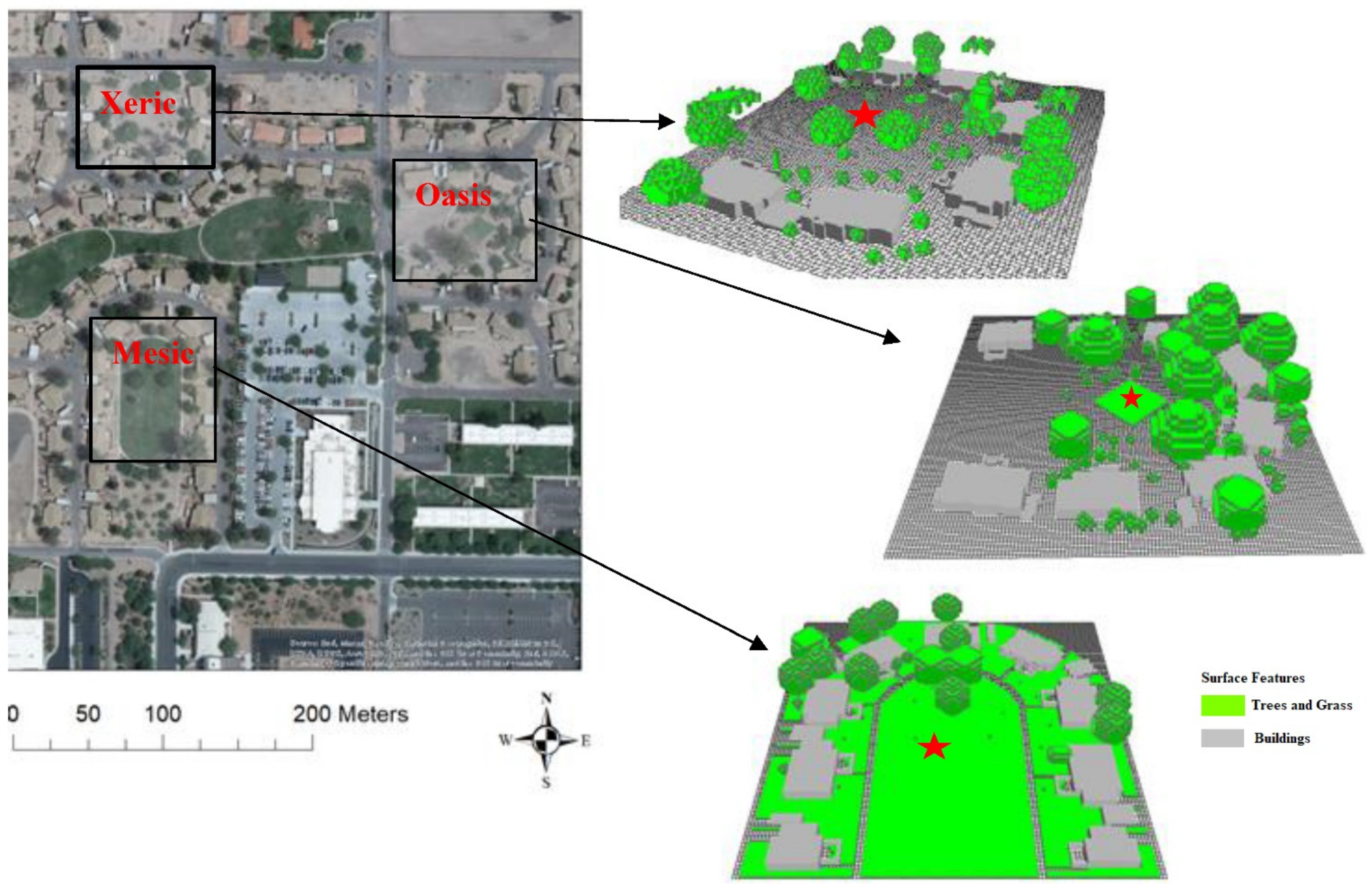
The North Desert Village (NDV) was used as a study area. It is located at Arizona State University’s Polytechnic campus and has three experimental sites with mesic, oasis, and xeric landscapes (Figure 1). The experimental sites were established in 2004 and designed to provide the Central Arizona–Phoenix Long-Term Ecological Research (CAP LTER) group a platform to study the plant–soil–water impacts of thermal and anthropogenic effects [37].
The mesic landscape site includes a mix of non-native and high water-use plants, trees, and turfgrass (green pixels, Figure 1). The oasis and xeric landscapes use non-native, desert-adapted species. Both neighborhoods are close to each other and have similar land covers, therefore, they fall in a similar local climate zone [38]. The mesic landscape site is mainly covered with turf grass and trees such as Acacia stenophylla, Malus, and Myrtus communis. The oasis landscape encompasses a patch of turf grass, shrubs, and trees surrounded by single-story residential buildings. Similarly, the xeric landscape was modeled with a density of shrubs, vines, and trees with a sparse leaf area. Each landscape has a micrometeorological station to monitor the air temperature at a 2 m height and the surface temperature, soil heat flux, and volumetric water content at a 30 cm depth. As presented in Figure 1 (red stars), the three stations are placed in the middle of the vegetated landscape. The station is placed at the top of the turfgrass in the mesic landscape and oasis landscape. The station was placed at top of the mulch surrounded by shrubs and trees in the xeric landscape. The three stations were under an open sky with no obstacles to create biases, however, some biases regarding the wind speed are inevitable because of the presence of hardscape and trees. The micrometeorological stations were used for the model validation.
3. Methodology
3.1. ENVI-Met Overview
ENVI-met is a three-dimensional CFD model used to simulate the physical processes of surface–plant–air interactions. It can model the ground conditions at spatial resolutions ranging between a 0.5 and 10 m grid cell size and a temporal resolution ranging between 24 and 48 h with a 1 to 5 s timestep [39]. The applications of ENVI-met range from simulating the urban heat island effects to evaluating vegetation densities in urban areas [36,39,40,41,42].
ENVI-met simulates 14 layers between the upper and 2 m deep layers. The soil layer is treated as a one-dimensional vertical column except for the upper layer, where heat transfer is calculated in three dimensions. The model calculates heat and water exchanges of soil at 0.01 m depth, close to the top layer of soil, and a depth of 0.5 m in the deeper layers up to 2 m. The introduced vegetation in the model is treated as a one-dimensional column with defined height. The model uses the leaf area density of the vegetation to define the distribution of the leaves. The soil model also works on a similar approach where the root area density (RAD) profile establishes the distribution of roots. The models’ detailed equations are presented by Bruse [42].
ENVI-met works on the principles of fluid dynamics, the fundamental laws of atmospheric physics, and thermodynamics. It is widely known to simulate surface–plant–air interactions in urban areas using atmospheric, surface, vegetation, and soil models. The atmospheric model calculates the three-dimensional turbulence, air movement, temperature, relative humidity, and variations in radiation due to shading and vegetated surfaces. The model solves the Reynolds averaged non-hydrostatic Navier–Stokes (RANS) equation in each grid cell for a defined time step [43]. The surface model calculates the heat exchanges of surfaces based on the residual energy of net radiation, soil heat flux, and sensible heat flux density [44]. Each nesting cell is represented by its thermodynamic model, having seven prognostic calculation nodes. The thermal state of the nodes is calculated from the physical properties of the wall/roof based on Fourier’s law of heat conduction. The vegetated model treats the plant’s canopy as aggregated dynamic objects reacting to the immediate environmental conditions [45]. This is done by modeling the exchange of CO2 and water vapor at the microscale (leaf level) using Jacob’s A-gs model, which, unlike Deardorff’s stomatal resistance model, considers the stomatal behavior of each leaf exposed to the heterogeneous microclimate conditions of plant and surroundings [37]. This allows an accurate simulation of plant physiological activity at the leaf scale, considering various environmental conditions. An observed relationship between the photosynthetic rate (An) of the plant and the stomatal conductance (gs) of the plant is used to observe the water use balance of plants and CO2 assimilation to minimize the water loss and maximize carbon gain [46]. The humidity response of the stomata in the model was estimated using the ratio of leaf internal CO2 concentration (Ci) to external concentrations (Cs). The basic principle of the model can be mathematically written as:
The value of 1.6 represents the diffusivity of CO2 and H2O in the air.
The physical limitation of ENVI-met regarding the vegetation modeling involves the oversimplification of the vegetation model. This was done to improve the computational efficiency. The ignored parameters include the attenuation of diffuse radiations, the reflectance of ground and vegetation surfaces, radiation heat transfer between the leaf, surface, and atmosphere, and the heat convection between the surrounding air and the surface area of the leaf [47]. Because of the oversimplification, the LAI is not climate-sensitive and has static values.
LAI has been widely tested for the hot desert climate but not for hot–humid climate zones. Recent studies have highlighted the limited application of ENVI-met in hot desert climates. Research in other climates have reported significant biases in vegetation modeling [48]. A study conducted to model the trees in sub-humid parts of Germany reported the underestimation of transpiration rates [49]. Another study compared the modeled and observed transpiration values and reported the improvement in performance if the input values of photosynthetic active radiation (PAR) were retrieved with minimal cloud cover [50]. Other studies have reported improvements in the performance of the tree model when the input LAI values were measured [51]. Therefore, this study has utilized the measured values. The details are provided in Section 3.2.
The ENVI-met database provides soil types and their profiles, plants, walls, and ground surfaces. The plant database includes a variety of tree species, hedges, and grasses, along with generic palm, deciduous, and coniferous trees of different sizes. The species are classified into high- and low-leaf-area density. ENVI-met allows the user to customize trees in an Albero tool to create a 3D plant based on its geometry, leaf area density, transmissivity, and biomass [52]. The soil database includes both marbled and natural soils, including loamy sand, basalt, cement concrete, and many more types. The limitation of the current ENVI-met version is that it only supports uniform building materials [29]. The profile database models the ground layers using a combination of soil types. It models a 200 cm deep ground layer. The profile database includes a range of surfaces, including loamy and sandy soil and different types of roads and pavements.
3.2. Model Setup
The model setup requires two major steps. First, the 3D model domain needs to be established through digitizing or importing data from shapefiles or Open Street Maps via Monde. Second, the meteorological forcing data for the day of interest must be defined in a simulation file, as well as other model parameters, such as the time step and simulation time.
While ENVI-met input data for buildings and ground surfaces were adopted from the study by Middel et al., 2014, the vegetation layer was replaced with 3D trees in ENVI-met version 4.4. The inventory for the species in each neighborhood is listed in Table 1. Based on the height and species of each tree in the ENVI-met 3.5 domain, a new 3D tree was selected from the ENVI-met database that most closely resembled the shape, type (coniferous vs. deciduous), and leaf area density (LAD) of the 2D tree. The plant species include 18 shrubs and 25 tree species, as presented in Table 1. The customization of each plant species was done in an Albero package of ENVI-met. The modeled trees were customized with a low leaf area density and an average height of 5 m. The inventory of plant species and their physiological properties was retrieved from various studies [13,53]. The studies used a plant canopy analyzer, namely LiCOR LAI-2000, to determine the leaf area of trees. The LAD was extrapolated using a regression model between the trees’ total foliage biomass and leaf area.
The selected soil parameters were retrieved from the Natural Resources Conservation Services (NRCS) database having Mohall Loam, consisting of clay loam, sandy loam, and loam [54]. We selected loamy sand from the ENVI-met 4.4 database as the soil in the model area. To simulate the ground conditions, the study used mulch (decomposing granite) for xeric and oasis landscapes. Mulch has a long history of being used in desert landscaping to reduce soil evaporation. Therefore, the non-turf grass surfaces were covered with a 5 cm layer of mulch. The soil characteristics of decomposing mulch were retrieved from previous studies in the North Desert Village [27,55]. Building walls were modeled as stucco with asphalt shingle roofs. In contrast to ENVI-met 3.5, version 4.4 allows for the hourly forcing of air temperature and humidity.
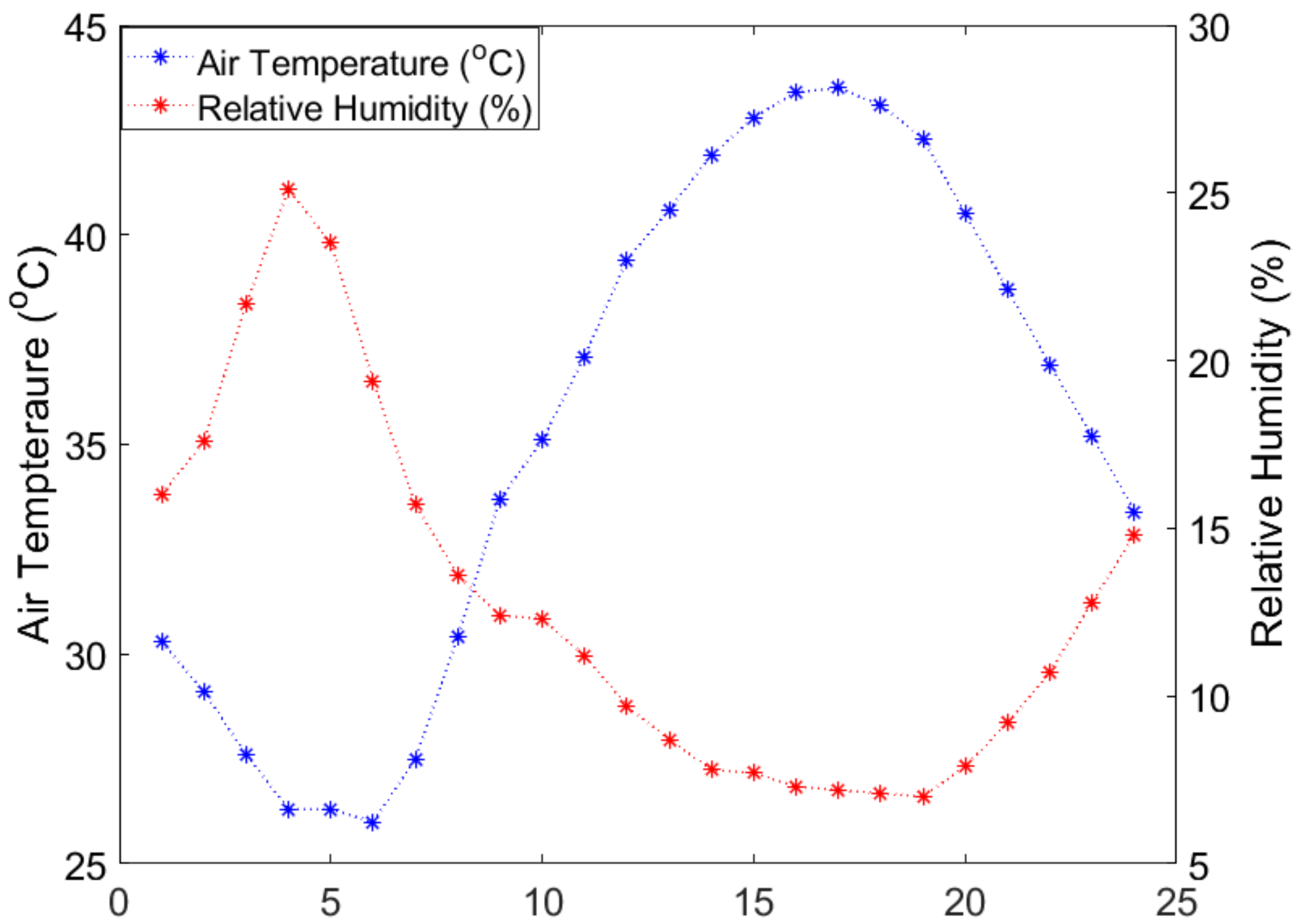
Forcing data were retrieved from the nearby Mesa airport (33.3090° N, 111.6559° W) (Figure 2). The airport site is 1.2 miles away from the study area; therefore, it was used as a site containing the initial boundary conditions for variables such as air temperature and relative humidity. No other stations were observed in the surrounding area, making the Mesa airport station the only option in the vicinity. The surface elevation is the main variable contributing to aberrant air temperature and relative humidity, which between the study area and the airport is flat, therefore, it was safe to consider the Mesa airport weather station dataset as an initial boundary condition.
The wind speed inputs for the model include those 10 m above wind speed, which was defined as 1.5 m/s NE at a roughness length from the reference point of 0.01 m.
3.3. Model Evaluation
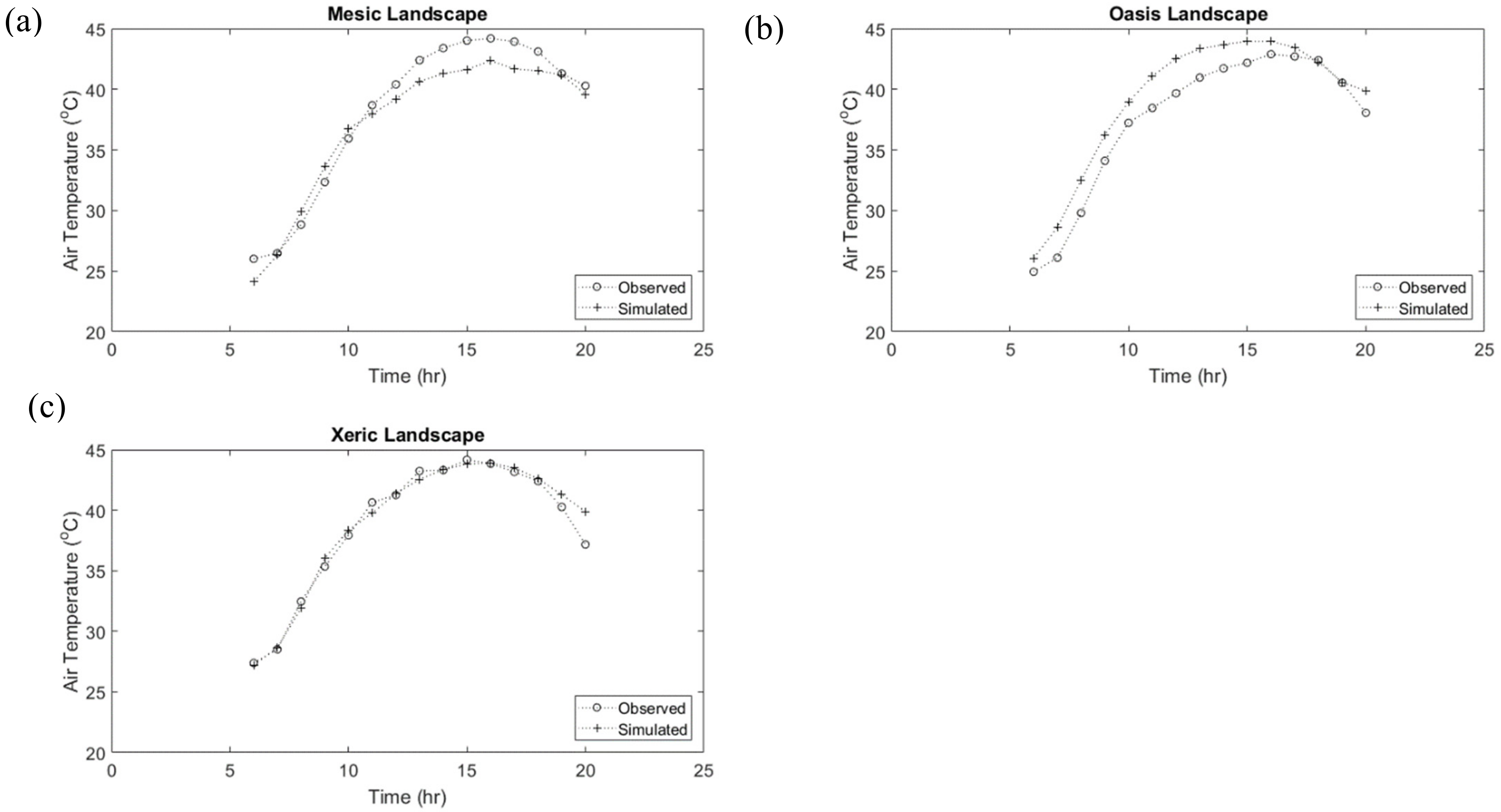
The model was evaluated by comparing the simulated hourly air temperature with the observed values. The study followed the methodology suggested by [56]. The experimental air temperature values were observed at 2 m above the surface and were acquired by installing a weather station at each landscape as part of the North Desert Village experiment (red stars in Figure 1 indicate the location). The simulated values were retrieved for the similar cell where the weather station was installed. The model calculates the values by introducing a receptor point. The deviation between the observed and simulated values was reported using root mean square error (RMSE) and mean absolute error (MAE). The bias in the model was calculated using mean bias error. The index of agreement between the observed and simulated data points was calculated to determine the degree to which the model was error-free. It ranged between zero and one; a value of d = 1 indicated that the simulated and observed values were error-free.
The simulated data were extracted at a receptor in the domain (red star, Figure 1). The model was validated by comparing the air temperature time series at 2 m with the simulated data points (Figure 3). Because of model spin-up time, the literature suggested using only the sunshine hours for validation [57,58,59]. Therefore, the validation was done for 15 h.
3.4. Determination of Microclimate Effects
Spatial maps and time series plots were created to understand the microclimate effects for the three landscapes. In this study, the microclimate effects were limited to the air temperature, surface temperature, and wind speed patterns in the three landscapes. These effects were investigated in an open sky setting and between buildings. A random set comprising twenty nesting grids of shrubs, turfgrass, and trees were considered. The twenty points around the landscape were selected to understand the microclimate effects of an open sky and shaded spaces in a neighborhood. This is because of the difference in the radiation budget in both surfaces. Typically, areas under shade have limited incident shortwave radiation, therefore, a lower surface temperature; however, some studies contest that the spaces could experience higher temperatures because of heat trapping induced by wall emissions [60,61]. The sampling was done for the open sky plants and between the buildings by defining various receptors and re-running the simulations. The time series of the nesting grids for different landscapes have been analyzed in the study.
3.5. Determination of Potential Irrigation Water Requirement
The potential irrigation water requirement is the function of evapotranspiration and irrigation efficiency. The evapotranspiration was estimated using the ENVI-met model. The values considered were the average of the cells in the open sky, while the irrigation efficiency was assigned based on the landscape type. The plant stomata in the model were given a zero value for the sunset hours. This means that the plant is highly stressed during the daytime, which may not be the case in the morning. However, the ENVI-met model did not respond well to daily patterns otherwise, with an unknown explanation. Future developments regarding the ENVI-met model can improve the daily stomatal response to water fluxes.
Irrigation efficiency is the ratio of water consumed by the plant to the water supplied through the irrigation system [62]. The xeric landscapes used drip irrigation, and its efficiency ranged between 75 and 90%. Because of the application of reclaimed water and leaching factors, the study considered a conservative approach and assigned 85% as irrigation efficiency [1]. The mesic landscape used sprinkler irrigation for the turfgrass, with an irrigation efficiency of 75%. An average of both the irrigation practices (80%) was assigned to the oasis landscape. Because the landscape utilized shrubs and trees and small parcels of the turfgrass, it was given a drip irrigation system.
The three landscapes were compared with cool-season grass, tall fescue, and Bermuda grass. The evapotranspiration of both grass types was higher than in the landscapes. The landscapes were compared to the two types of grass to understand the differences that were observed due to the mixed species.
4. Results
4.1. Model Evaluation
Overall, the three landscapes conform to the ground conditions, as shown in Figure 3. The xeric landscape led to a high RMSE of 1.92 °C (Table 2). The second highest value was observed for the mesic landscape (1.50 °C), followed by the oasis landscape (0.86 °C) (Table 2). The ENVI-met tool reportedly performed poorly in the xeric landscape, which was designed for temperate climates [12,26].
4.2. Microclimate Effects of Landscapes
To explain the microclimate conditions, this section is divided into three subsections. In the first subsection, variations of surface temperature at noon in the mesic, oasis, and xeric landscapes are explained through spatial maps. The second subsection describes the spatial variations of wind speeds through 3D spatial maps provided for the mesic, oasis, and xeric landscapes. The third subsection provides the diurnal air temperature variation and wind speed at two meters. An open-sky vegetated surface and the vegetated surface between the buildings were considered for the diurnal effects. The diurnal variations are explained using a line graph.
4.2.1. Variation in Surface Temperature
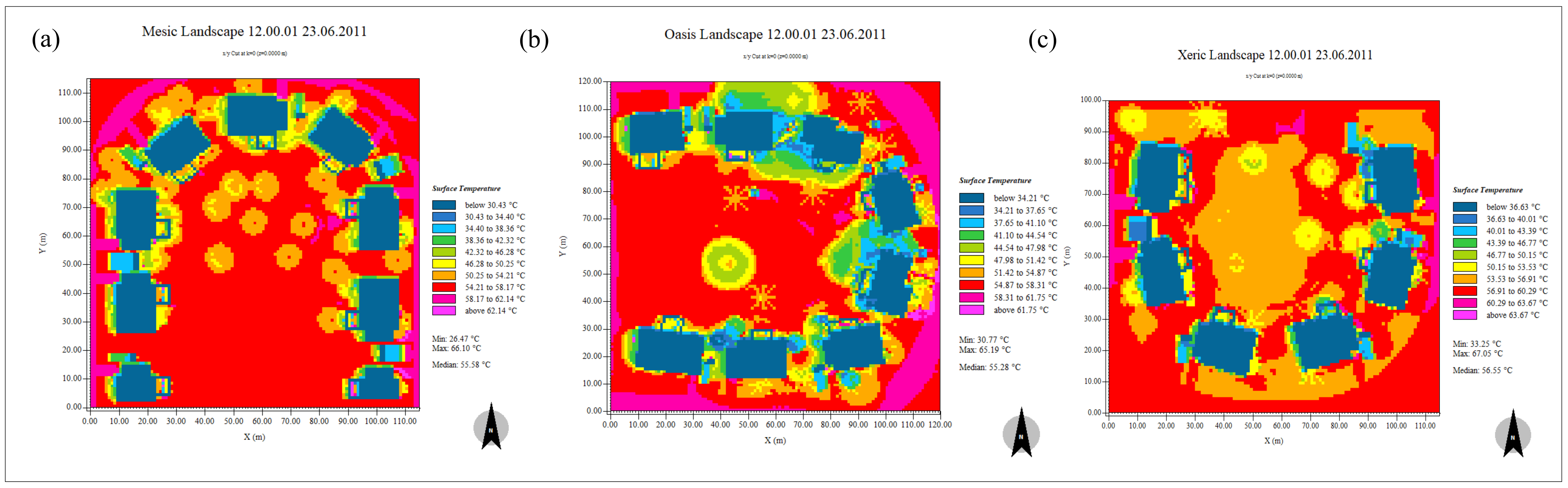
The building height, soil type, and soil profile are the same for the three landscapes. The three landscapes are in the same local climate zone and are less than one mile from one another. Therefore, it is safe to assume that the diurnal surface temperature variations are due to the surface energy exchanges. Figure 4 shows the surface temperature variations of the three types of landscapes at noon. The blue color shows a lower temperatures, while red and pink show higher temperatures.
Figure 4a shows the mesic landscape with eleven single-story buildings of a five-meter height, surrounded by trees and turfgrass. The highest temperature in the landscape was reported as being 66 °C, visible at the border of the neighborhood (pink spots). In contrast, the lowest temperature reported was 26 °C, observed for the shaded surfaces between the buildings. A median value of 55.5 °C was observed for the landscape. Additionally, the characters with tree shade (orange pixels) show a 4 °C lower surface temperature than the turfgrass surfaces (red pixels). The lowest temperature was observed for the surfaces that had both engineered shade (buildings and overhang) and tree shade (cyan pixels). An 8 °C difference in temperature was observed between the characters under tree shade and engineered shade. In addition, a difference of 4 °C was observed between the turfgrass surfaces with and without tree shade.
The average surface temperature of the oasis landscape is comparable to the mesic landscape, as shown in Figure 4b. However, the lowest temperature observed in the landscape was 5 °C higher (31 °C), and the maximum temperature was 1 °C lower (65 °C) than the mesic landscape. The highest temperature was observed for the hardscapes (pink and red pixels) at the outskirts, while the surfaces between the buildings and under the tree shade showed lower temperatures (yellow and green pixels). In addition, the surfaces between the buildings were 4–9 °C cooler than the open-sky surfaces, as visible in Figure 4b.
The xeric landscape was 1 °C warmer in terms of average surface temperatures than the mesic and oasis landscapes (Figure 4c). The maximum surface temperature at the neighborhood border was 1 °C higher than the mesic landscape and 2 °C lower than the oasis landscape. The minimum surface temperature was 7 °C higher than the mesic landscape and 3 °C higher than the oasis landscape.
Overall, the variations in minimum surface temperature can be inferred from the cooling due to the different landscapes. The cooling effects were higher for the mesic landscape because of its tree/turf landscape. The xeric landscape contributed relatively less to cool the surface.
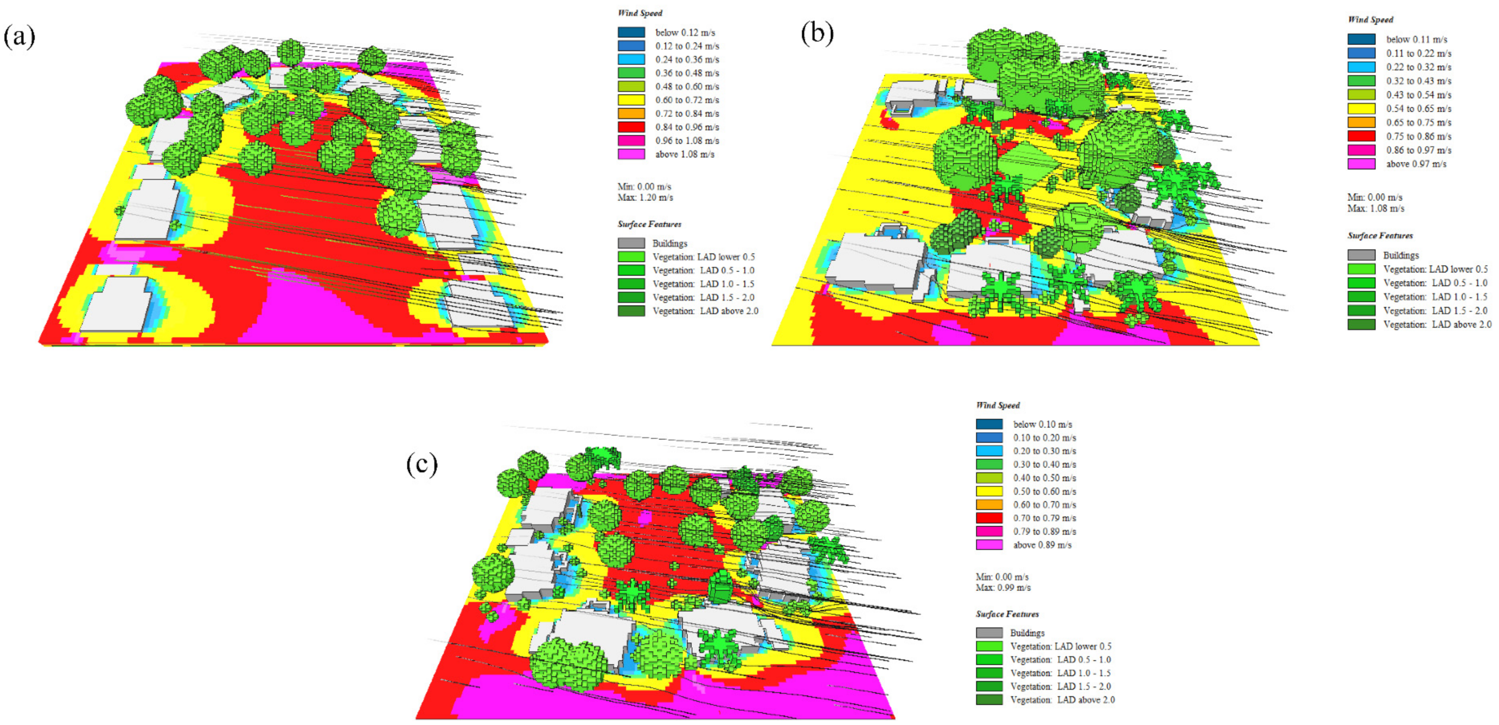
4.2.2. Spatial Variation in Wind Speed
Figure 5 presents a 3D view of the landscapes with surface features and wind speed. The presence of buildings and trees reduced the wind speed by breaking kinetic energy, causing turbulence [63]. In the mesic landscape, the maximum wind speed was reported as 1.20 m/s (pink and red pixels), and the minimum wind speed was 0.6 m/s (cyan and yellow pixels), as shown in Figure 5a. The mesic landscape was modeled with high-leaf-area density shrubs and trees, ranging between 15 and 25 m. The increased wind speed was observed at the neighborhood border, while the low wind speeds were observed surrounding the buildings and trees.
In the case of the oasis landscape, the wind speed was higher for the surfaces between the buildings and trees, as shown in Figure 5b. The landscape was modeled with spherical trees, having a crown of 15 m and a depth of 20 m. The difference was 0.1 m/s between the surfaces obstructed by the buildings and the open sky.
The xeric landscape was modeled with low-leaf-area density and spherical trees and shrubs ranging between 5 and 15 m (Figure 5c). Relative to the two landscapes, the xeric landscapes showed lower wind speeds. However, the wind speed within the buildings was 0.3 m/s higher than the oasis landscape and 0.1 m/s more than the mesic landscape.
4.2.3. Diurnal Variation in Air Temperature and Wind Speed
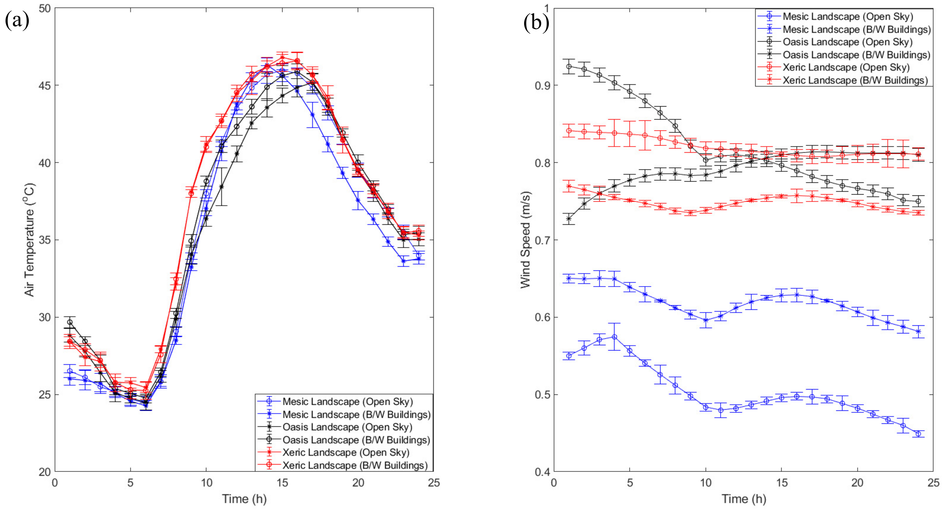
Figure 6a shows the average behavior of the air temperature for the mesic, oasis, and xeric landscapes. The turfgrass surfaces were considered for the air temperature response. Turfgrass within the open sky and surrounded by buildings and trees was reported. This was done to understand the thermal effects of the presence of the buildings and trees. The peak air temperature was observed at 15:00 h with 48 °C. The lowest air temperature was kept at 6:00 h (25 °C). Overall, no significant difference was observed for the vegetated surfaces with an open sky or between buildings.
The lower air temperature was observed for the mesic landscape. This behavior was expected. However, the mesic landscape showed a 2 °C higher air temperature during peak daytime hours (11:00 h–13:00 h) for the surfaces between buildings. This effect can be induced by the emissions of the wall surfaces, causing heat-trapping.
The oasis landscape showed a similar pattern of air temperature variation to the mesic landscape. However, interestingly, the air temperature of the open-sky surface between 11:00–13:00 h was 1 °C lower than in the mesic landscape. Furthermore, a drop in air temperature (2 °C) was observed for prolonged periods (10:00–16:00) in the oasis neighborhood between buildings. However, the nighttime air temperature was observed to be similar to the xeric landscape.
The xeric landscape showed, on average, a 3 °C higher temperature than the mesic and xeric landscapes. The xeric landscape employed low-water-consuming plant species with a sparse leaf area density. This reduces the transpiration rates and increases air temperatures. The air temperature of the xeric landscape showed the same behavior in an open sky and between surfaces.
Figure 6b shows the overall landscapes’ wind speed. The variations in the wind speeds are inconclusive. An open-sky vegetated patch in the mesic landscape has a lower wind speed than oasis and xeric landscapes. Similarly, the mesic landscape’s wind speed between the buildings (canyon effects) is lower than the xeric and mesic landscapes. The wind speeds are a function of the geometry of the structure, including the tree height, crown cover, and canopy cover of trees and bushes, respectively, along with building heights [21,64,65]. Therefore, lower wind speed rates may be explained due to the presence of more trees breaking the wind energy. However, the orientations of the three landscapes are entirely different, which makes the findings questionable, hence inconclusive. In this study, real neighborhoods were considered; wind patterns can be a challenge. Ideal research to understand wind variations can be done using ENVI-met by devising a hypothetical neighborhood with the same orientation, soil profile, and building density to understand the wind patterns.
4.3. Potential Irrigation Water Requirement of Landscapes
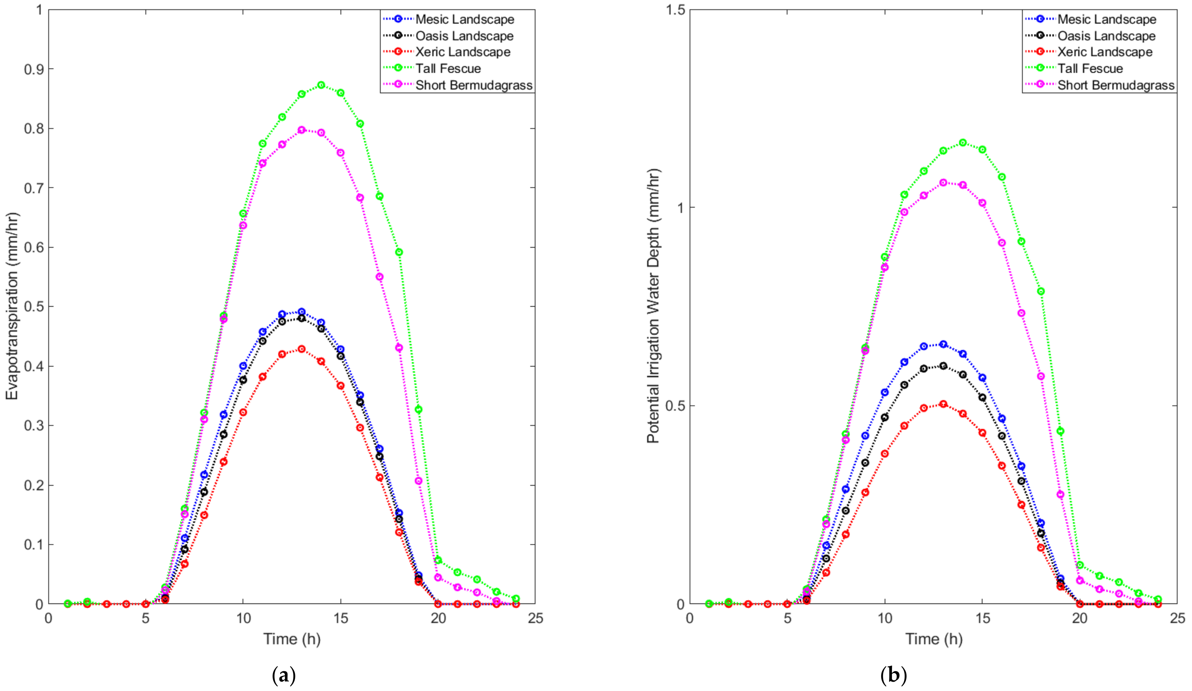
The irrigation water requirements of the landscapes were estimated as a function of evapotranspiration and irrigation efficiency. The values of evapotranspiration are the average over the landscape. Overall, the mesic landscape showed higher evapotranspiration values, followed by the oasis and xeric landscapes, as shown in Figure 7. The evapotranspiration rates were highest between 11 and 12 h, followed by a steep drop in the afternoon (13:00–15:00 h). This diurnal effect was similar throughout the three landscapes. The oasis landscape showed lower evapotranspiration rates (~0.3 mm/h) than the mesic landscape. The xeric landscape showed overall lower evapotranspiration throughout the day, with, on average, a 0.5 mm/h lower evapotranspiration rate than the mesic landscape and a 0.3 mm/h lower than the oasis landscape.
The study compared the evapotranspiration of mesic, oasis, and xeric landscapes with tall fescue grass and Bermuda grass to understand the variations in the irrigation water compared to an entire turf landscape. The comparison of evapotranspiration with tall fescue showed a 50% decrease in evapotranspiration, while the oasis and xeric landscapes showed a 52 and 56% decrease in evapotranspiration, respectively (Figure 7a). In a similar way, the comparison of landscapes with short Bermuda grass showed a decrease of 43, 46, and 53% in the mesic, oasis, and xeric landscapes, respectively.
The potential irrigation water depths were estimated as a function of evapotranspiration and irrigation efficiency. The irrigation depth of the mesic landscape was slightly higher than the oasis landscape (~0.1 mm/h), as presented in Figure 7b. However, the xeric landscape showed 0.5 mm/h lower irrigation water depth than the xeric and mesic landscapes. The irrigation water depth of landscapes when compared to tall fescue was lower, with 50, 55, and 64% decreases in the mesic, oasis, and xeric landscapes, respectively. Similarly, the comparison of irrigation water depth between short Bermuda grass and landscapes showed a respective reduction of 43, 49, and 59 for the mesic, oasis, and xeric landscapes.
5. Discussion
This study hypothesized that the ET and IWR would be lower for xeric landscapes, categorized as a low-water-use landscape. As the decreased ET induces higher daytime air temperature, it was assumed that higher daytime cooling would be reported by the mesic landscape, having higher ET. The results support the hypotheses. A 5-year study by Sovocool (2005) in Las Vegas, NV, reported similar findings, with 76% water savings in single-family houses because of the xeric landscape when compared to the mesic landscape.
Another hypothesis was that the ET of turfgrass would be higher than tree transpiration. Bermuda grass and fescue ET were 43% higher than the mesic landscape; therefore, the results confirm the hypothesis. In addition, the results corroborated sufficiently with previous studies with similar hypotheses. For instance, a study reported the summertime ET of turfgrass at between 2 and 6 mm/day, while the tree transpiration remained less than 1 mm/day [21]. The study was conducted in the Los Angeles metropolitan area, in California, an arid region, using portable cuboid chamber measurements (in situ approach). The findings reinforce the smart water landscape (WSL) programs approach, focused on reducing per capita demand by removing turfgrass. However, the long-term water benefits of replacing the turfgrass with WSL and synthetic turf grass remain unclear. In another study, twelve-year monthly water consumption records were analyzed for 300,000 households in Las Vegas, Nevada, and estimated the average water saving per square meter of turf removed [66]. The study reported no evidence of water savings per unit area being influenced by the rebate value. Not enough literature is available to corroborate the irrigation values of the three landscapes in arid regions. Most of the literature quantifies the irrigation water requirement of individual species [67,68]. However, one study estimated the irrigation schedules of xeric and mesic landscapes for monthly use. By the process of deduction, the study found comparable values of irrigation for mesic (4–6 mm/day) and xeric (2–3 mm/day) landscapes [32].
A significant limitation of this study was a relatively coarse approach towards the irrigation system. The study utilized the irrigation efficiency values from the literature. The irrigation water requirement is attributed to both ET and irrigation efficiency. One study highlights that 66% of water savings due to xeric landscape is attributed to precise irrigation systems [1]. Another limitation is the constant diurnal wind regime [26]. The ENVI-met considers average wind speed and uses hourly forcing to prepare daily spatial wind profiles. Future studies can focus on assessing modeled and calculated wind speed accuracy by installing an anemometer at 2 m. In addition, ENVI-met does not allow for the correct distribution of irrigation water requirements unless the stomatal opening at the daytime is set to zero, which translates into stressed plants. This may not always be true, especially in climates with high relative humidity creating more biases.
Regardless of the limitations, this study can assist water managers in understanding the water requirements of mesic landscapes, compared to xeric and oasis landscapes. In addition, the study highlights the implication of Water Smart Landscape programs and is significant to urban climate scientists. It highlights the importance of changes in surface temperature and air temperature due to mesic, xeric, and oasis landscapes and their response to increased water requirements of plant species. In addition, the study emphasizes the role of buildings and trees in lowering wind speed.
6. Conclusions
This study simulated three typical landscapes in an arid region to understand the microclimate conditions and irrigation water requirements. The goal was to determine a microclimate and irrigation water-efficient landscape. Three landscapes, including mesic, oasis, and xeric, were studied. The microclimate effects were determined by analyzing the spatial maps and diurnal plots of surface temperature, wind speed, and air temperature. The landscapes were modeled using the North Desert Village plant data with an ENVI-met tool. Previous studies have determined the changes in air and surface temperature in the landscapes; this study is an extension as it provided the irrigation water requirements and the intra-urban microclimate changes due to vegetation. The tool utilizes building and atmospheric physics algorithms to determine the plant–soil–atmosphere interactions. The landscapes were simulated for 24 h for the hottest day of the year, i.e., 23 June 2011, using Phoenix, AZ’s climate data.
Even though the study is specific to three landscapes, the findings can be generalized into irrigation water responses of tree turf landscapes and low water use species. The study modeled forty-three species, including trees and shrubs. In addition, the study utilized a desert climate for the initial boundary conditions. Therefore, with a few exceptions such as wind speed variations and relative humidity, the findings for irrigation water depths can be translated for an arid climate such as those in Las Vegas and Los Angeles.
Findings suggest oasis landscapes are 5 °C warmer on average, concerning surface temperatures, than mesic landscapes. The xeric landscape was 1 °C warmer than the mesic and oasis landscapes over the hardscapes. Additionally, the vegetated surfaces for the xeric landscape were 7 °C warmer than the mesic and oasis landscapes.
The findings regarding the wind speed differences are inconclusive as wind speed inherently depends on a range of factors. Since this study utilized actual landscapes, various factors were beyond control, including the orientation of the buildings and the trees’ geometry in the landscape (tree height and building height). Therefore, findings such as those for mesic landscapes, with tall trees (height-5–10 m), demonstrating lower wind speeds, especially between buildings and trees, remain inherently flawed. Future studies can focus on devising an experiment using inputs from the study in a hypothetical neighborhood with constant geometrical parameters to understand the wind speed variations.
Overall, the mesic landscape induced a cooling effect. However, the surfaces between buildings were 2 °C warmer than the surrounding area at noon, indicating heat-trapping. On the other hand, the oasis landscape showed a 2 °C lower air temperature than the mesic landscape at the peak daytime. However, the oasis landscape showed a nighttime air temperature similar to that of the xeric landscape.
The potential evapotranspiration of the mesic landscape was highest, followed by the oasis and xeric landscapes. The oasis landscape shows, on average, a 0.1 mm/h reduction in the depth of irrigation. The xeric landscape reports the lowest depth for irrigation.
To conclude, the oasis landscape contributes to maximum daytime cooling along with lower irrigation water requirements when compared to the mesic landscape. The xeric landscape saves irrigation water; however, it does not promise outdoor thermal comfort, including reduced air temperature or dense shading.
Author Contributions
R.S. was involved in the conceptualization, formal analysis, methodology, visualization, writing-the original draft. A.M. provides the resources, supervision, and methods of the study. H.S. and S.A. participated in the conceptualization, methodology, resources, and management of the study. All authors have read and agreed to the published version of the manuscript.
Funding
This research was funded by the University of Nevada, Las Vegas, under the Top Tier Doctoral Graduate Research Assistantship (TTDGRA) program. R.S.’s contribution was also partly supported by the Maki postdoctoral fellowship at the Desert Research Institute.
Data Availability Statement
Part of the data used is from [27]. The Mesic, Oasis, and Xeric landscape database is available at the given repository: http://0-doi-org.brum.beds.ac.uk/10.5281/zenodo.5015501. The software used for the analysis was ENVI-met version 4.4.1 and had restricted access.
Acknowledgments
The authors are grateful to Dale Devitt, at the Department of Life Sciences, University of Nevada, Las Vegas, for his rigorous reviews and meaningful comments.
Conflicts of Interest
The authors declare no conflict of interest.
References
- Hilaire, R.S.; Arnold, M.A.; Wilkerson, D.C.; Devitt, D.A.; Hurd, B.H.; Lesikar, B.J.; Lohr, V.I.; Martin, C.A.; McDonald, G.V.; Morris, R.L.; et al. Efficient water use in residential urban landscapes. HortScience 2008, 43, 2081–2092. [Google Scholar] [CrossRef]
- Brelsford, C.; Abbott, J.K. How Smart Are ‘Water Smart Landscapes’? 2018, pp. 1–45. Available online: http://arxiv.org/abs/1803.04593 (accessed on 13 March 2018).
- Pincetl, S.; Gillespie, T.W.; Pataki, D.E.; Porse, E.; Jia, S.; Kidera, E.; Nobles, N.; Rodriguez, J.; Choi, D.A. Evaluating the effects of turf-replacement programs in Los Angeles. Landsc. Urban Plan. 2019, 185, 210–221. [Google Scholar] [CrossRef]
- Sovocool, K.A. Xeriscape Conversion Study Final Report by Area. 2005, p. 93. Available online: http://www.allianceforwaterefficiency.org/Xeriscape_Water_Savings.aspx (accessed on 10 April 2020).
- Fisher, J.B.; Whittaker, R.J.; Malhi, Y. ET come home: Potential evapotranspiration in geographical ecology. Glob. Ecol. Biogeogr. 2011, 20, 1–18. [Google Scholar] [CrossRef]
- OKE, T.R. The energetic basis of the urban heat island. Q. J. R. Meteorol. Soc. 1987, 16, 121–129. [Google Scholar] [CrossRef]
- Saher, R.; Ahmad, S.; Stephen, H. Analysis of changes in surface energy fluxes due to urbanization in Las Vegas. In Proceedings of the World Environmental and Water Resources Congress 2019: Groundwater, Sustainability, Hydro-Climate/Climate Change, and Environmental Engineering, Pittsburgh, PA, USA, 19–23 May 2019; American Society of Civil Engineers: Reston, VA, USA, 2019. [Google Scholar] [CrossRef]
- Wood, L.; Hooper, P.; Foster, S.; Bull, F. Public green spaces and positive mental health—Investigating the relationship between access, quantity and types of parks and mental wellbeing. Health Place 2017, 48, 63–71. [Google Scholar] [CrossRef] [PubMed]
- Saher, R.; Stephen, H.; Ahmad, S. Urban evapotranspiration of green spaces in arid regions through two established approaches: A review of key drivers, advancements, limitations, and potential opportunities. Urban Water J. 2020, 18, 1–13. [Google Scholar] [CrossRef]
- Smeal, D.; O’Neill, M.; Lombard, K.; Arnold, R. Crop Coefficients for Drip-Irrigated Xeriscapes and Urban Vegetable Gardens; NMSU Agricultural Science Center: Los Lunas, NM, USA, 2009; pp. 1–12. [Google Scholar]
- Kjelgren, R.; Rupp, L.; Kilgren, D. Water conservation in urban landscapes. HortScience 2000, 35, 1037–1040. [Google Scholar] [CrossRef] [Green Version]
- Chow, W.T.; Brazel, A.J. Assessing xeriscaping as a sustainable heat island mitigation approach for a desert city. Build. Environ. 2012, 47, 170–181. [Google Scholar] [CrossRef]
- Middel, A.; Chhetri, N.; Quay, R. Urban forestry and cool roofs: Assessment of heat mitigation strategies in Phoenix residential neighborhoods. Urban For. Urban Green. 2015, 14, 178–186. [Google Scholar] [CrossRef]
- Mitchell, D. Assessment of the Viability of Xeriscaping to Reduce Water Consumption in Sacramento. Unpublished work. 2014. [Google Scholar]
- Overview, W.V. Offsetting water conservation costs to achieve net-zero water use. J. Am. Water Work. Assoc. 2013, 105, 62–72. [Google Scholar] [CrossRef]
- Saher, R. Kaleidoscope of Urban Evapotranspiration: Exploring the Science and Modeling Approaches. Doctoral Dissertation, University of Nevada, Las Vegas, NV, USA, 2021. [Google Scholar]
- Nouri, H.; Beecham, S.; Kazemi, F.; Hassanli, A.M. A review of ET measurement techniques for estimating the water requirements of urban landscape vegetation. Urban Water J. 2013, 10, 247–259. [Google Scholar] [CrossRef]
- Saher, R.; Stephen, H.; Ahmad, S. Urban Climate “Urban Climate Effect of land use change on summertime surface temperature, albedo, and evapotranspiration in Las Vegas Valley”. Urban Clim. 2021, 39, 100966. [Google Scholar] [CrossRef]
- Saher, R.; Stephen, H.; Ahmad, S. Urban Climate Understanding the summertime warming in canyon and non-canyon surfaces. Urban Clim. 2021, 38, 100916. [Google Scholar] [CrossRef]
- Litvak, E.; Manago, K.F.; Hogue, T.S.; Pataki, D.E. Evapotranspiration of urban landscapes in Los Angeles, California at the municipal scale. Water Resour. Res. 2017, 53, 4236–4252. [Google Scholar] [CrossRef]
- Litvak, E.; Bijoor, N.S.; Pataki, D.E. Adding trees to irrigated turfgrass lawns may be a water-saving measure in semi-arid environments. Ecohydrology 2014, 7, 1314–1330. [Google Scholar] [CrossRef]
- Litvak, E.; Pataki, D.E. Evapotranspiration of urban lawns in a semi-arid environment: An in situ evaluation of microclimatic conditions and watering recommendations. J. Arid Environ. 2016, 134, 87–96. [Google Scholar] [CrossRef] [Green Version]
- Kusaka, H.; Kimura, F. Coupling a Single-Layer Urban Canopy Model with a Simple Atmospheric Model: Impact on Urban Heat Island Simulation for an Idealized Case. J. Meteorol. Soc. Japan 2004, 82, 67–80. [Google Scholar] [CrossRef] [Green Version]
- Chen, F.; Kusaka, H.; Bornstein, R.; Ching, J.; Grimmond, C.S.B.; Grossman-Clarke, S.; Loridan, T.; Manning, K.W.; Martilli, A.; Miao, S.; et al. The integrated WRF/urban modelling system: Development, evaluation, and applications to urban environmental problems. Int. J. Climatol. 2011, 31, 273–288. [Google Scholar] [CrossRef]
- Vahmani, P.; Hogue, T.S. Incorporating an Urban Irrigation Module into the Noah Land Surface Model Coupled with an Urban Canopy Model. J. Hydrometeorol. 2014, 15, 1440–1456. [Google Scholar] [CrossRef]
- Crank, P.J.; Middel, A.; Wagner, M.; Hoots, D.; Smith, M.; Brazel, A. Validation of seasonal mean radiant temperature simulations in hot arid urban climates. Sci. Total Environ. 2020, 749, 141392. [Google Scholar] [CrossRef]
- Middel, A.; Häb, K.; Brazel, A.J.; Martin, C.A.; Guhathakurta, S. Impact of urban form and design on mid-afternoon microclimate in Phoenix Local Climate Zones. Landsc. Urban Plan. 2014, 122, 16–28. [Google Scholar] [CrossRef]
- Vahmani, P.; Sun, F.; Hall, A.; Ban-Weiss, G. Investigating the climate impacts of urbanization and the potential for cool roofs to counter future climate change in Southern California. Environ. Res. Lett. 2016, 11, 124027. [Google Scholar] [CrossRef]
- Crank, P.J.; Sailor, D.J.; Ban-Weiss, G.; Taleghani, M. Evaluating the ENVI-met micro-scale model for suitability in analysis of targeted urban heat mitigation strategies. Urban Clim. 2018, 26, 188–197. [Google Scholar] [CrossRef]
- Kjelgren, R.; Beeson, R.C.; Pittenger, D.P.; Montague, T. Simplified landscape irrigation demand estimation: Slide rules. Appl. Eng. Agric. 2016, 32, 363–378. [Google Scholar] [CrossRef]
- Hoedjes, J.C.B.; Chehbouni, A.; Jacob, F.; Ezzahar, J.; Boulet, G. Deriving daily evapotranspiration from remotely sensed instantaneous evaporative fraction over olive orchard in semi-arid Morocco. J. Hydrol. 2008, 354, 53–64. [Google Scholar] [CrossRef] [Green Version]
- Volo, T.J.; Vivoni, E.R.; Ruddell, B.L. An ecohydrological approach to conserving urban water through optimized landscape irrigation schedules. Landsc. Urban Plan. 2015, 133, 127–132. [Google Scholar] [CrossRef]
- Litvak, E.; McCarthy, H.R.; Pataki, D.E. Transpiration sensitivity of urban trees in a semi-arid climate is constrained by xylem vulnerability to cavitation. Tree Physiol. 2012, 32, 373–388. [Google Scholar] [CrossRef] [Green Version]
- Litvak, E.; McCarthy, H.R.; Pataki, D.E. A method for estimating transpiration of irrigated urban trees in California. Landsc. Urban Plan. 2017, 158, 48–61. [Google Scholar] [CrossRef] [Green Version]
- Nouri, H. Evapotranspiration estimation in heterogeneous urban vegetation. Doctoral Dissertation, University of South Australia, Adelaide, Australia, 2014. [Google Scholar]
- Ambrosini, D.; Galli, G.; Mancini, B.; Nardi, I.; Sfarra, S. Evaluating mitigation effects of urban heat islands in a historical small center with the ENVI-Met® climate model. Sustainability 2014, 6, 7013–7029. [Google Scholar] [CrossRef] [Green Version]
- Sarijeva, G.; Knapp, M.; Lichtenthaler, H.K. Differences in photosynthetic activity, chlorophyll and carotenoid levels, and in chlorophyll fluorescence parameters in green sun and shade leaves of Ginkgo and Fagus. J. Plant Physiol. 2007, 164, 950–955. [Google Scholar] [CrossRef]
- Stewart, I.D.; Oke, T.R. Local climate zones for urban temperature studies. Bull. Am. Meteorol. Soc. 2012, 93, 1879–1900. [Google Scholar] [CrossRef]
- Ozkeresteci, I.; Crewe, K.; Brazel, A.J.; Bruse, M. Use and evaluation of the ENVI-MET model for enviromental design and planning: An experiment on linear parks. In Proceedings of the 21st International Cartographic Conference (ICC), Durban, South Africa, 10–16 August 2003; pp. 10–16. [Google Scholar]
- Zhao, Q.; Sailor, D.J.; Wentz, E.A. Impact of tree locations and arrangements on outdoor microclimates and human thermal comfort in an urban residential environment. Urban For. Urban Green. 2018, 32, 81–91. [Google Scholar] [CrossRef] [Green Version]
- Taleghani, M.; Kleerekoper, L.; Tenpierik, M.; Van Den Dobbelsteen, A. Outdoor thermal comfort within five different urban forms in the Netherlands. Build. Environ. 2015, 83, 65–78. [Google Scholar] [CrossRef]
- Bruse, M. ENVI-met 3.0: Updated Model Overview. System 2004, 1–12. [Google Scholar]
- Berardi, U.; Jandaghian, Z.; Graham, J. Science of the Total Environment Effects of greenery enhancements for the resilience to heat waves: A comparison of analysis performed through mesoscale (WRF) and microscale (Envi-me) modeling. Sci. Total Environ. 2020, 747, 141300. [Google Scholar] [CrossRef]
- Toparlar, Y.; Blocken, B.; Maiheu, B.; Van Heijst, G.J.F. A review on the CFD analysis of urban microclimate. Renew. Sustain. Energy Rev. 2017, 80, 1613–1640. [Google Scholar] [CrossRef]
- Simon, H.; Lindén, J.; Hoffmann, D.; Braun, P.; Bruse, M.; Esper, J. Modeling transpiration and leaf temperature of urban trees—A case study evaluating the microclimate model ENVI-met against measurement data. Landsc. Urban Plan. 2018, 174, 33–40. [Google Scholar] [CrossRef]
- Gibelin, A.L.; Calvet, J.C.; Roujean, J.L.; Jarlan, L.; Los, S.O. Ability of the land surface model ISBA-A-gs to simulate leaf area index at the global scale: Comparison with satellites products. J. Geophys. Res. Atmos. 2006, 111, 1–16. [Google Scholar] [CrossRef]
- Liu, Z.; Zheng, S.; Zhao, L. Evaluation of the ENVI-Met Vegetation Model of Four Common Tree Species in a Subtropical Hot-Humid Area. Atmosphere 2018, 9, 198. [Google Scholar] [CrossRef] [Green Version]
- Asef, S.M.; Tolba, O.; Fahmy, A. The effect of leaf area index and leaf area density on urban microclimate. J. Eng. Appl. Sci. 2020, 67, 427–446. [Google Scholar]
- Simon, H. Modeling Urban Microclimate: Development, Implementation and Evaluation of New and Improved Calculation Methods for the Urban Microclimate Model ENVI-Met; Universitätsbibliothek Mainz: Mainz, Germany, 2016. [Google Scholar]
- Lindén, J.; Simon, H.; Fonti, P.; Esper, J.; Bruse, M. Observed and Modeled transpiration cooling from urban trees in Mainz, Germany. In Proceedings of the ICUC9-9th International Conference on Urban Climate Jointly with 12th Symposium on the Urban Environment, Toulouse, France, 20–24 July 2015; pp. 20–24. [Google Scholar]
- Huttner, S. Further Development and Application of the 3D Microclimate Simulation ENVI-met. Doctoral Dissertation, Johannes Gutenberg-Universitat in Mainz, Mainz, Germany, 2012; p. 147. Available online: http://ubm.opus.hbz-nrw.de/volltexte/2012/3112/ (accessed on 11 October 2021).
- Mohsen, H.; Raslan, R.M.; El-Bastawissi, I. Optimising the Urban Environment through Holistic Microclimate Modelling: The Case of Beirut’s Peri-Center Faculty of Architectural Engineering; Beirut Arab University, Lebanon UCL Institute for Environmental Design and Engineering (IEDE), The Bar: Beirut, Lebanon, 2015. [Google Scholar]
- Lalic, B.; Mihailovic, D.T. An empirical relation describing leaf-area density inside the forest for environmental modeling. J. Appl. Meteorol. 2004, 43, 641–645. [Google Scholar] [CrossRef]
- Soil Surveys by State NRCS Soils. Available online: https://www.nrcs.usda.gov/wps/portal/nrcs/surveylist/soils/survey/state/?stateId=AZ (accessed on 19 February 2022).
- Singer, C.K.; Martin, C.A. Effect of Landscape Mulches and Drip Irrigation on Transplant Establishment and Growth of Three North American Desert Native Plants. J. Environ. Hortic. 2009, 27, 166–170. [Google Scholar] [CrossRef]
- Willmott, C.J. On the validation of models. Phys. Geogr. 1981, 2, 184–194. [Google Scholar] [CrossRef]
- Battista, G.; Carnielo, E.; Vollaro, R.D.L. Thermal impact of a redeveloped area on localized urban microclimate: A case study in Rome. Energy Build. 2016, 133, 446–454. [Google Scholar] [CrossRef]
- Lin, B.S.; Lin, C.T. Preliminary study of the influence of the spatial arrangement of urban parks on local temperature reduction. Urban For. Urban Green. 2016, 20, 348–357. [Google Scholar] [CrossRef]
- Zhang, Y.; Murray, A.T.; Turner Ii, B.L. Landscape and Urban Planning Optimizing green space locations to reduce daytime and nighttime urban heat island e ff ects in Phoenix, Arizona. Landsc. Urban Plan. 2017, 165, 162–171. [Google Scholar] [CrossRef]
- Shashua-Bar, L.; Hoffman, M.E. Geometry and orientation aspects in passive cooling of canyon streets with trees. Energy Build. 2003, 35, 61–68. [Google Scholar] [CrossRef]
- Shashua-Bar, L.; Pearlmutter, D.; Erell, E. The influence of trees and grass on outdoor thermal comfort in a hot-arid environment. Int. J. Climatol. 2011, 31, 1498–1506. [Google Scholar] [CrossRef]
- Jensen, R.R.; Hardin, P.J.; Bekker, M.; Farnes, D.S.; Lulla, V.; Hardin, A. Modeling urban leaf area index with AISA+ hyperspectral data. Appl. Geogr. 2009, 29, 320–332. [Google Scholar] [CrossRef]
- Fisher, J.B.; Baldocchi, D.D.; Misson, L.; Dawson, T.E.; Goldstein, A.H. What the towers don’t see at night: Nocturnal sap flow in trees and shrubs at two AmeriFlux sites in California. Tree Physiol. 2007, 27, 597–610. [Google Scholar] [CrossRef] [Green Version]
- Chatzidimitriou, A.; Yannas, S. Microclimate design for open spaces: Ranking urban design effects on pedestrian thermal comfort in summer. Sustain. Cities Soc. 2016, 26, 27–47. [Google Scholar] [CrossRef]
- Pataki, D.E.; McCarthy, H.R.; Litvak, E.; Pincetl, S. Transpiration of urban forests in the Los Angeles metropolitan area. Ecol. Appl. 2011, 21, 661–677. [Google Scholar] [CrossRef] [Green Version]
- Brelsford, C.; Abbott, J.K. Growing into Water Conservation? Decomposing the Drivers of Reduced Water Consumption in Las Vegas, NV. Ecol. Econ. 2017, 133, 99–110. [Google Scholar] [CrossRef]
- Volo, T.J.; Vivoni, E.R.; Martin, C.A.; Earl, S.; Ruddell, B.L. Modelling soil moisture, water partitioning, and plant water stress under irrigated conditions in desert Urban areas. Ecohydrology 2014, 7, 1297–1313. [Google Scholar] [CrossRef]
- Kim, J.; Hogue, T.S. Evaluation of a MODIS triangle-based evapotranspiration algorithm for semi-arid regions. J. Appl. Remote Sens. 2013, 7, 073493. [Google Scholar] [CrossRef] [Green Version]
Figure 1.
Study area showing the mesic, oasis, and xeric landscape with their surface features; red stars in each landscape indicate the weather station used for the model validation.
Figure 1.
Study area showing the mesic, oasis, and xeric landscape with their surface features; red stars in each landscape indicate the weather station used for the model validation.

Figure 2.
ENVI-met weather input (hourly) for 23 June 2011.

Figure 3.
Model evaluations by comparing the observed and simulated air temperature at 2 m height for mesic (a), oasis (b), and xeric (c) landscapes.
Figure 3.
Model evaluations by comparing the observed and simulated air temperature at 2 m height for mesic (a), oasis (b), and xeric (c) landscapes.

Figure 4.
Surface temperatures of the mesic (a), oasis (b), and xeric (c) landscapes at noon.

Figure 5.
Wind speeds for mesic (a), oasis (b), and xeric (c) landscapes at noon.

Figure 6.
(a) Diurnal variation of air temperatures for the landscapes; (b) diurnal variation of wind speeds for the landscapes.
Figure 6.
(a) Diurnal variation of air temperatures for the landscapes; (b) diurnal variation of wind speeds for the landscapes.

Figure 7.
(a) Evapotranspiration rates of the landscapes; (b) potential irrigation water depths of the landscapes.
Figure 7.
(a) Evapotranspiration rates of the landscapes; (b) potential irrigation water depths of the landscapes.


Table 1.
Trees, shrubs, and vines in the study area were modeled using 2D plants in ENVI-met 3.5.
| Species Biological Name | Mesic Landscape | Oasis Landscape | Xeric Landscape |
|---|---|---|---|
| Trees | |||
| Acacia Salonica | • | ||
| Acacia stenophylla | • | • | • |
| Brachychiton populneus | • | ||
| Brahea armata | • | ||
| Corymbia papuana | • | ||
| Eucalyptus camaldulensis | • | • | |
| Eucalyptus microtheca | • | ||
| Eucalyptus polyanthemos | • | ||
| Fraxinus under | • | ||
| Fraxinus valutina | • | ||
| Malus (apple) | • | ||
| Melaleuca viminalis | • | • | • |
| Myrtus communis | • | • | |
| Parkinsonia hybrid | • | ||
| Phoenix dactylifera | • | • | • |
| Pinus eldarica | • | • | |
| Pinus halepensis | • | ||
| Pistacia chinesis | • | ||
| Platanus wrightii | • | ||
| Platycladus orientalis | • | • | • |
| Prosopis hybrid | • | ||
| Prunus cerasifera | • | ||
| Ulmus parvifolia | • | • | |
| Washingtonia filifera | • | ||
| Shrubs and Vines | |||
| Bougainvillea hybrid | • | ||
| Caesalpinia pulcherrima | • | ||
| Caesalpinia gilliesii | • | ||
| Calliandra californica | • | ||
| Carissa macrocarpa | • | ||
| Chamaerops humilis | • | ||
| Encelia farinosa | • | ||
| Hesperaloe parviflora | • | ||
| Lantana hybrid | • | ||
| Leucophyllum candidum | • | ||
| Leucophyllum frutescens | • | ||
| MacFadyena unguis-cati | • | ||
| Myrtus communis | • | • | |
| Nerium oleander | • | • | |
| Rosa hybrid | • | ||
| Ruellia brittoniana | • | ||
| Ruellia peninsularis | • | ||
| Tacoma capensis | • | ||
• modeled in the landscape.
Table 2.
Model evaluation using basic statistics between observed and simulated air temperatures at 2 m.
Table 2.
Model evaluation using basic statistics between observed and simulated air temperatures at 2 m.
| Model Parameters | Mesic | Xeric | Oasis |
|---|---|---|---|
| RMSE | 1.50 | 0.86 | 1.92 |
| MBE | 0.91 | 0.21 | 1.69 |
| MAE | 1.33 | 0.56 | 1.70 |
| d | 0.98 | 1.00 | 1.00 |
Publisher’s Note: MDPI stays neutral with regard to jurisdictional claims in published maps and institutional affiliations. |
© 2022 by the authors. Licensee MDPI, Basel, Switzerland. This article is an open access article distributed under the terms and conditions of the Creative Commons Attribution (CC BY) license (https://creativecommons.org/licenses/by/4.0/).
Share and Cite
MDPI and ACS Style
Saher, R.; Middel, A.; Stephen, H.; Ahmad, S. Assessing the Microclimate Effects and Irrigation Water Requirements of Mesic, Oasis, and Xeric Landscapes. Hydrology 2022, 9, 104. https://0-doi-org.brum.beds.ac.uk/10.3390/hydrology9060104
AMA Style
Saher R, Middel A, Stephen H, Ahmad S. Assessing the Microclimate Effects and Irrigation Water Requirements of Mesic, Oasis, and Xeric Landscapes. Hydrology. 2022; 9(6):104. https://0-doi-org.brum.beds.ac.uk/10.3390/hydrology9060104
Chicago/Turabian StyleSaher, Rubab, Ariane Middel, Haroon Stephen, and Sajjad Ahmad. 2022. "Assessing the Microclimate Effects and Irrigation Water Requirements of Mesic, Oasis, and Xeric Landscapes" Hydrology 9, no. 6: 104. https://0-doi-org.brum.beds.ac.uk/10.3390/hydrology9060104
Note that from the first issue of 2016, this journal uses article numbers instead of page numbers. See further details here.