
What Is the Contribution of Urban Trees to Mitigate Pluvial Flooding?


1
Institute of Hydrology and Water Resources Management, Leibniz Universität Hannover, 30167 Hannover, Germany
2
Climate Service Center Germany (GERICS), Helmholtz-Zentrum Hereon, 21502 Hamburg, Germany
3
Institute of Physical Geography and Landscape Ecology, Leibniz Universität Hannover, 30167 Hannover, Germany
*
Author to whom correspondence should be addressed.
†
These authors contributed equally to this work.
Hydrology 2022, 9(6), 108; https://0-doi-org.brum.beds.ac.uk/10.3390/hydrology9060108
Submission received: 11 May 2022
/
Revised: 31 May 2022
/
Accepted: 14 June 2022
/
Published: 16 June 2022
(This article belongs to the Special Issue Urban Flood Mitigation and Stormwater Management)
Abstract
:Hydrological modeling is commonly used in urban areas for drainage design and to estimate pluvial flood hazards in order to mitigate flood risks and damages. In general, modelers choose well-known and proven models, which are tailored to represent the runoff generation of impervious areas and surface runoff. However, interception and other vegetation-related processes are usually simplified or neglected in models to predict pluvial flooding in urban areas. In this study, we test and calibrate the hydrological model LEAFlood (Landscape and vEgetAtion-dependent Flood model), which is based on the open source ‘Catchment Modeling Framework’ (CMF), tailored to represent hydrological processes related to vegetation and includes a 2D simulation of pluvial flooding in urban areas using landscape elements. The application of LEAFlood was carried out in Vauban, a district in Freiburg (Germany) with an area of ∼31 hectares, where an extensive hydrological measurement network is available. Two events were used for calibration (max intensity 17 mm/h and 28 mm/h) and validation (max intensity 25 mm/h and 14 mm/h), respectively. Moreover, the ability of the model to represent interception, as well as the influence of urban trees on the runoff, was analyzed. The comparison of observed and modeled data shows that the model is well-suited to represent interception and runoff generation processes. The site-specific contribution of each single tree, approximately corresponding to retaining one cup of coffee per second (∼0.14 L/s), is viewed as a tangible value that can be easily communicated to stakeholders. For the entire study area, all trees decrease the peak discharge by 17 to 27% for this magnitude of rainfall intensities. The model has the advantage that single landscape elements can be selected and evaluated regarding their natural contribution of soil and vegetation to flood regulating ecosystem services.
1. Introduction
Hydrological models are important tools in planning and for research and being increasingly used. Often, modelers choose well-known and proven rainfall-runoff models [1], which are tailored to represent the runoff generation of impervious areas and surface runoff. However, hydrological models that also adequately represent and include vegetation are rare, and more modeling studies on this topic are needed [2]. An overview of modeling tools that analyze the impact of trees on hydrology is presented by Coville et al. [3]. In summary, the authors highlight the diverging range of complexity of models involved, ranging from tree-scale models to catchment-scale models [3].
The vast majority of models that predict the extent of pluvial flooding focus on 2D hydrology-hydrodynamics with a simplified representation of interactions with vegetation in predicting runoff generation [4,5,6]. Moreover, typical ‘stormwater’ models—rainfall-runoff models designed for urban areas—used to predict hydrological processes in urban areas also simplify hydrology-vegetation interactions and focus on surface runoff over impervious surfaces, thus suggesting further improvements of model components [7,8]. However, models that include a better representation of vegetation in hydrology mostly operate at the catchment scale [9,10,11,12]—a scale, which is too coarse to study the impact of single trees at a quarter scale. Hence, a better representation of both vegetation and 2D routing would be preferable to study the effect of different types of stormwater measures. For this very reason and in view of the fact that using an existing model based on earlier experience is not necessarily the best choice [13], a model is needed that fulfills the following characteristics:
- Simple 2D-hydrodynamics to predict the extent of pluvial flooding in urban areas,
- Detailed representation of hydrology–vegetation interactions (i.e., interception).
These research gaps bring up the following research questions: (i) Can we parameterize a hydrological model that is capable of predicting both interception processes and the spatio-temporal extent of pluvial flooding at the same time? (ii) What is the role of (single) trees in retaining heavy rainfall at the quarter scale? In order to bridge the gap between very detailed 2D hydrological-hydrodynamic models and catchment-scale hydrological models that are capable of predicting vegetation interactions, a model tailored to these requirements is used and tested in this study. Furthermore, in order to benefit from proven and existing model components, the model (LEAFlood—Landscape and vEgetAtion-dependent Flood model) we applied is based on the Catchment Model ling Framework (CMF) [14]. Among numerous other applications, this framework has already been used to study the storage of green roofs [15]. In the present study, LEAFlood allows us to combine the benefits of a detailed canopy and interception representation together with a 2D surface routing based on the kinematic wave approximation. For calibration of urban hydrological models, runoff measurements are needed, however, these data are rare in ungauged urban areas [16]. The urban district Vauban in Freiburg (Germany) provides a comprehensive measuring network of hydrological variables, i.e., runoff and canopy throughfall among others. In order to overcome the challenge of calibration and plausibility checks in urban areas, the datasets from Vauban are used to validate LEAFlood.
The objectives of this paper are to (i) test and calibrate a model that accounts for both detailed vegetation interactions with hydrology during heavy rainfall events and a 2D surface runoff simulation. After model set-up and calibration, we demonstrate the added value of the model and (ii) estimate the role of trees in runoff generation during pluvial flooding at the quarter scale.
After this introduction, the materials and methods are presented. These include the study area, the data, the model LEAFlood, the calibration set up and procedure for the model experiments with different tree coverage. The results and discussion follow in a combined chapter. It is divided into sub-chapters about the model performance for interception, the surface runoff calibration and the results of the model experiments with different tree coverage to study “the role of trees in pluvial flooding”. The chapter ends with a section about limitations before going on to the conclusions and outlook.
2. Materials and Methods
2.1. Study Area
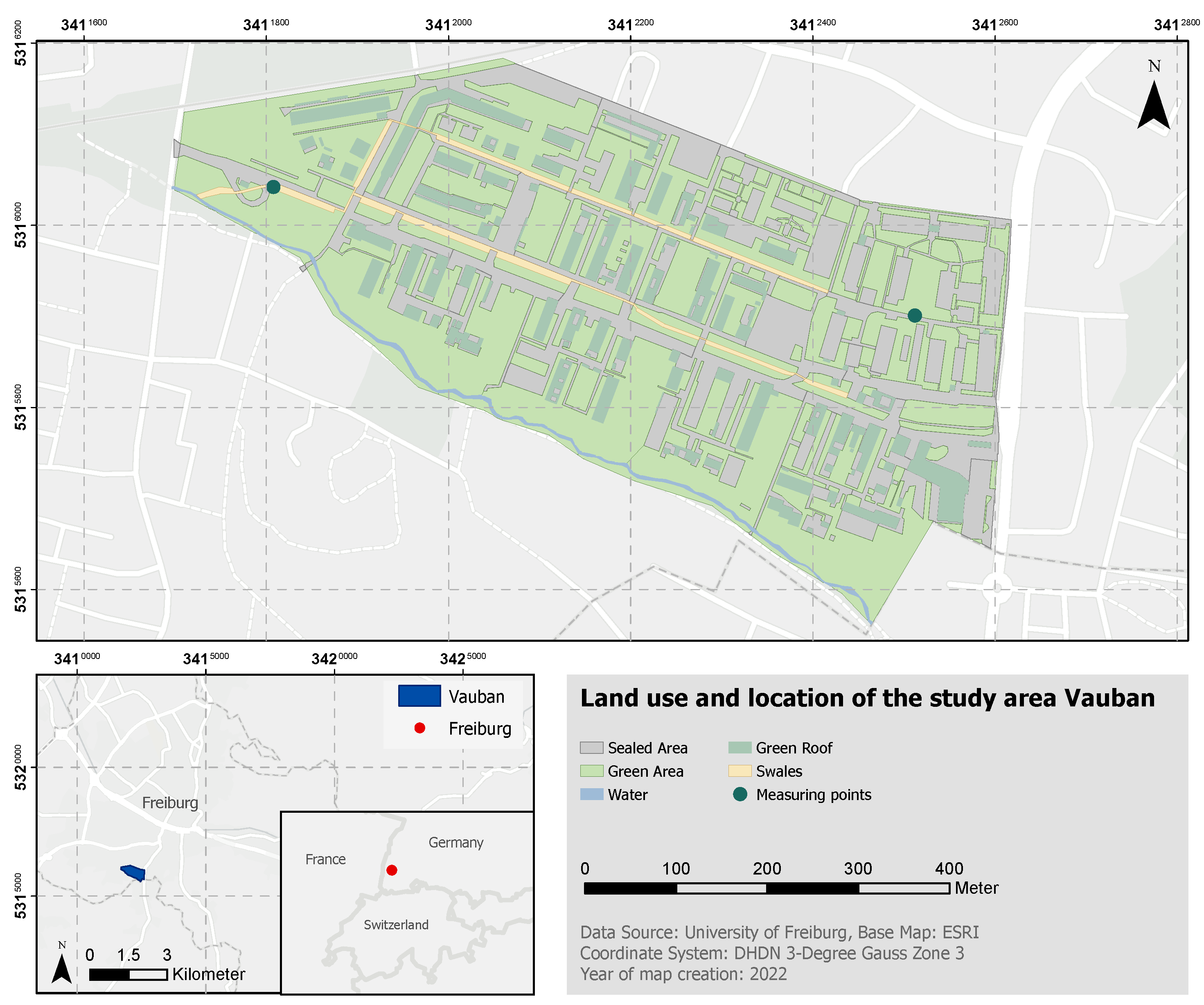
The research area is located in the Vauban district of Freiburg, Germany and has an area of 30.8 ha (Figure 1). It is a residential area with an estimated of 5500 inhabitants [17]. The area was chosen due to its detailed hydrological measuring network that is available within the urban area, installed to monitor the performance of its drainage system, which has already been used in various studies [18,19]. This measurement dataset is used to calibrate and validate the LEAFlood model.
The climate conditions in the region are maritime to semi-continental. The mean annual precipitation is 934 mm (1981–2010) at the DWD Freiburg station [20] (∼5.4 km from study area, which is used to analyze climate conditions, while local measurements are available for further analyses). The dominant land use type in the zone are green areas (65.3%), including vegetative swales and green roofs. The remaining area is covered by sealed urban areas (33.8%) and a water body (1%). Around 14% of the district is covered by tree canopies. The main soil types are loam and sandy loam [19,21,22] (data adopted from the UrbanRoGeR model).
The study site was developed on a former French military base from the 20th century. After an urban design competition, a maximization on Green Infrastructure (GI) (Notwithstanding the broad range of terms used similarly [23], such as, e.g., Low Impact Development (LID) [18], water smart cities etc. [24], the term GI is used here for simplicity) was achieved [25]. The winning urban plan included extensive green areas, making most of the roofs green, walking paths with permeable pavements, rainwater harvesting and incentives for intensive private gardening [17]. The generated runoff of the area is collected and redirected to a central Infiltration-Swale System (ISS). The ISS consists of individual swales connected as cascade by pipes under the streets, forming two parallel lines along the main streets (Nordgraben, Boulevardgraben). A downstream swale collects the discharge of both lines, redirecting the overflow via an intake structure into the receiving watercourse. The downstream swale drains as a free overflow to the downstream part of the Dorfbach creek, located along the southern border of the district, which flows from southeast to west.
2.2. Data
Meteorological data and geodata are required for the application of the model. Table 1 shows a detailed overview of the used datasets, their resolution and sources. The Digital Elevation Model (DEM), tree coverage and soil class map are used to define the geometry and parameters of cells (a term adopted from CMF, i.e., a polygon) in LEAFlood. The climate data, such as precipitation and temperature, determine the meteorological conditions during the event, whereas the measured records (runoff and interception) are used for calibration and evaluation of the model performance. Rainfall has been recorded on-site with a heated tipping bucket rain gauge with 0.1 mm resolution [18]. Regarding the number of tree units, these allow us to quantify the contribution of individual urban trees to reduce runoff generation. Lime tree (tilia), plane tree (platanus) and, to a smaller degree, firs (abies) are the prevailing tree species for which interception—or more specifically throughfall—measurements exist in the study area. Throughfall is measured through a tipping bucket rain gauge, which is mounted under the tree’s canopy.
2.3. LEAFlood (Landscape and vEgetAtion-Dependent Flood Model)
The LEAFlood model [29] is based on existing model components of the Catchment Modelling Framework (CMF) [14,30]. CMF is not a ready-to-use model, but a programming library for hydrological modeling that allows for the development of models tailored to various research questions in hydrology. The modular structure of this open source Python package provides high flexibility and is adaptable to different research questions. It is written in C++ and uses the finite volume method [14]. It thus fills the gap needed for a modular and flexible hydrological model framework. This is especially important for hydrological modeling in urban areas and the reason why we chose this framework [8,31]. With CMF it is possible to create polygon cells out of a GIS shapefile in the required spatial resolution in order to overcome the aforementioned limitation: CMF allows to develop a model that accounts for both a detailed representation of interception and a lateral 2D surface runoff simulation. In addition, the hydrological processes can be selected from a range of different approaches depending on the research question, as demonstrated for physically-based hydrological modeling of green roofs based on CMF [15]. This makes the package very suitable for a spatially explicit analysis of flood regulating ecosystem services supply in urban areas.
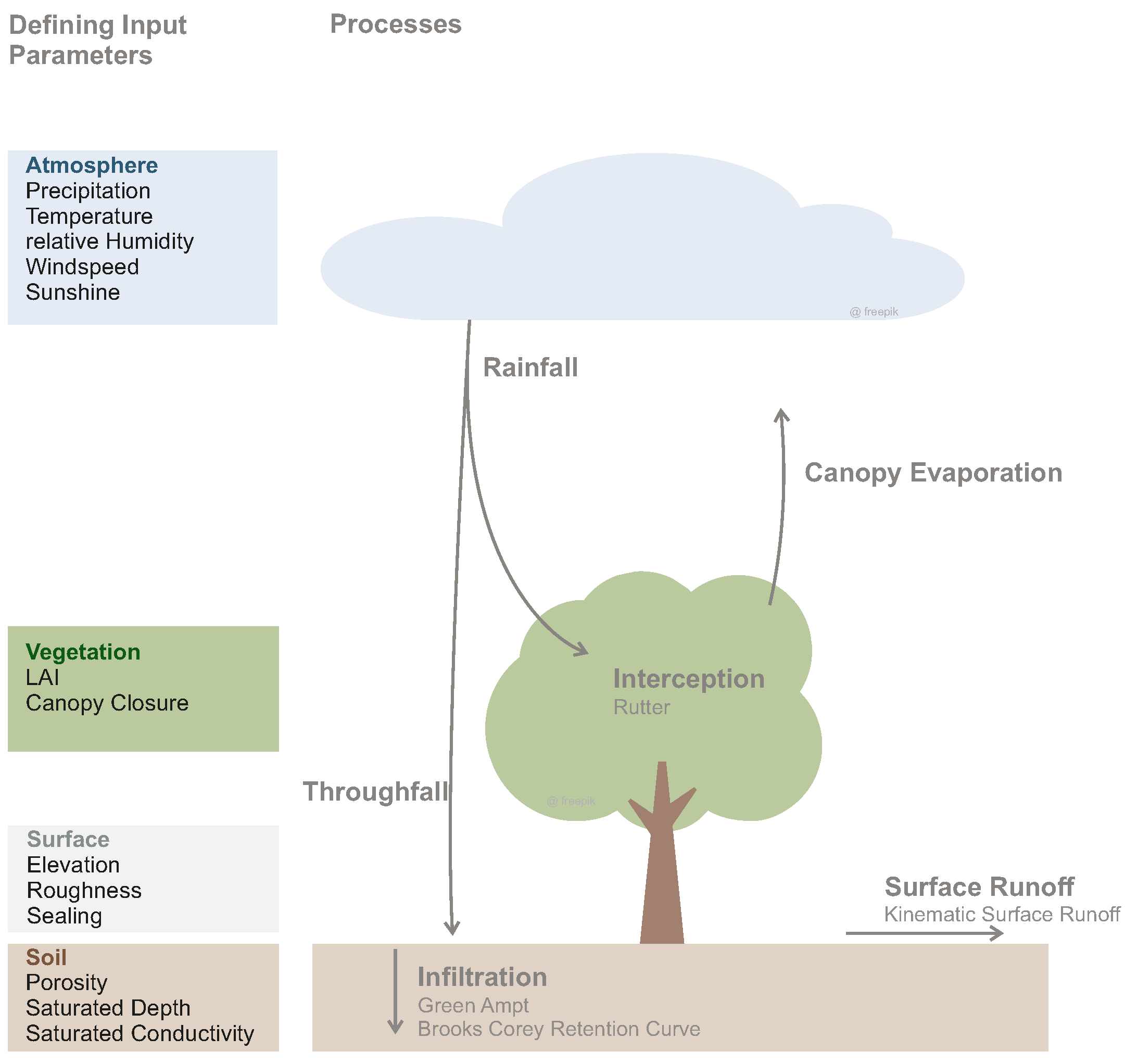
LEAFlood considers the hydrological processes of canopy interception, throughfall, soil infiltration and surface runoff (Figure 2). Evaporation from the canopy is regarded in the model, while evapotranspiration and evaporation from the surface is neglected. This limitation is accepted in this study, as the model is designed to be utilized for single heavy rainfall events (e.g., [32]), during which canopy evaporation is expected to be the dominant evaporative loss among all evapotranspiration fluxes. The geometry is created on the basis of an irregular polygon shapefile.
The model is driven by meteorological data of rainfall, temperature, wind speed, relative humidity and solar radiation in a five-minute resolution. The interception utilises the Rutter approach [30,33]. Depending on the canopy closure, the precipitation can either be intercepted in the canopy or fall directly to the ground. A canopy closure of 1 means all rain is intercepted and 0 indicates throughfall [30]. To define the canopy closure of each cell, we used a polygon shapefile with the tree canopy in the area and intersect it with its corresponding cell’s location. The quotient of the canopy area and cell area equals the canopy closure. Average LAI and interception capacity were defined representative for all trees.
The soil consists of one soil layer with the Green-Ampt infiltration method and the Brooks-Corey Retention Curve. It is assumed that during heavy precipitation events only the upper layer plays a role in infiltration and that percolation does not due to the time decay. Except for saturated conductivity (), all other parameters are the same throughout the study area (Table 2). The base value for Ksat is 0.3 m/d resulting from the soil property sandy loam and the dry bulk density 4 + 5 [34]. Depending on the degree of soil sealing, is reduced by the following function:
A higher degree of sealing therefore results in a lower value. The porosity of sandy loam is 0.453 [34]. Because of soil compaction in urban areas the value is reduced to 0.3 [35]. The surface runoff follows the kinematic approach based on topography and surface roughness [30]. Manning’s roughness coefficient is defined for each land use class (Table 3).
With these components, LEAFlood entails a level of describing hydrological processes, which is in between a conceptual and physically-based, distributed, deterministic model description [36].
2.4. Calibration
In order to achieve a reasonable calibration of the model, two events are selected (Table 4) and a split-sample test is employed [37] to assess the model calibration through an independent validation with two further events. The selection of the events is based on the highest precipitation intensities observed over the 2 years of available data. The rainfall events for calibration reach a maximum intensity of 16.5 mm/h with a return period of less than one year (event 1) and 28 mm/h (return period ∼5 years) for event 2 (return periods refer to the study of Shehu et al. [38]). Similar intensities can be observed for event 3 and 4, which are used for validation. Event 3 has a maximum intensity of 25 mm/h (return period between 1–5 years) and event 4 has a maximum intensity of 14 mm/h (return period less than 1 year). Besides runoff, interception is also observed by throughfall measurements. The accuracy of interception measurements is checked before model calibration. As the throughfall is measured instead of interception storage , a simple bucket model is employed to compute interception from observed rainfall and throughfall :
where i denotes the time step, is the storage computed for the previous time step, and the rate of evaporation losses from the canopy, which is neglected (i.e., ). Since the interception model in CMF and LEAFlood has no adjustable parameters, the model performance of interception modelling is assessed before calibrating other hydrological processes similar to Förster et al. [39]. It is assumed that a reasonable representation of interception processes justifies calibrating only those model parameters of runoff generation that govern hydrological processes below the canopy.
Given a sufficient accuracy in interception modeling, processes related to runoff generation below the canopy are considered, mainly parameters governing infiltration. These are the parameter b of the Brooks–Corey retention curve and two scaling parameters that allow for adjusting Manning’s roughness n and saturated hydraulic conductivity , respectively. The latter two parameters are factors applied to the roughness and conductivity values for each polygon.
In order to calibrate the model according to the split-sample test, an objective function is introduced first, which consists of two components. The first component is the Nash–Sutcliffe model efficiency E, which is computed for observed q and predicted runoff [40], given that each time series consists of N time steps i:
A second component, the relative difference in peak discharge over events, is introduced in order to give more emphasis on peak runoff in the calibration procedure:
2.5. Model Experiments with Different Tree Coverage
The quantification of the impact of trees on hydrological processes in the study area, mainly the impact on pluvial flooding, is performed utilizing two model experiments for each event. First, the calibrated model is used to study the hydrological response of the study area covered by trees ‘as is’. Second, a similar run—but with a zero tree coverage—is performed to study the hydrological response of the same event without any trees. Since both runs only differ in terms of tree coverage, it is possible to quantify the role of trees through a comparison of both runs [39].
3. Results and Discussion
3.1. Interception
The first step in our model evaluation pertains to analyzing the model interception component. For three types of trees (lime tree (tilia), plane tree (platanus), and fir (abies)), throughfall was recorded in the study area. However, we focus on the lime tree only, since the plane tree is similar in terms of throughfall and firs with higher interception storage rarely occur in the study area, making them less representative.
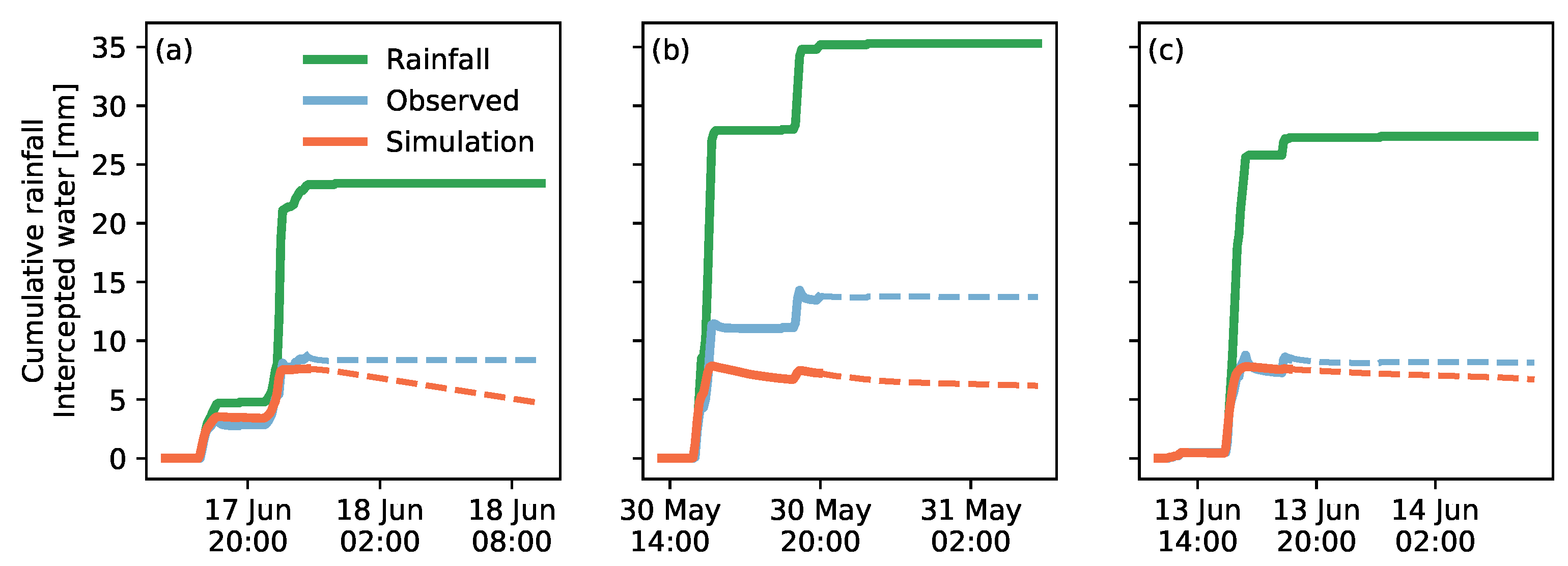
The interception storage, computed utilizing Equation (2), for each time step during the first three events are compiled in Figure 3. Since evaporation is neglected, making Equation (2) valid for the rainfall event only, the dry period after each event is indicated as dashed lines, for which the comparison is subject to the aforementioned limitation. In general, the temporal evolution of intercepted load (intercepted water/storage) is represented well by the model. This holds true for both the timing of increments in interception storage and its absolute values over time. Only for event 2 is interception slightly underestimated by 5 mm at the end of the event, while for event 4, no interception measurements are available. However, given the overall high accuracy of predicting interception, the model is capable of representing interception during rainfall events.
Interception is subject to uncertainties related to the characteristics of individual trees, which influence the interception amount [2,43]. Here, the location and the coverage of the trees are known. However, we neither have detailed information about the spatial distribution of tree species nor about individual LAI and interception capacities. Therefore, we assume a mean LAI and interception capacity for all trees. Furthermore, the seasonality of trees governs the annual course of LAI and interception capacity [44]. This seasonal dependence is not considered in this study, which is accepted, since all events considered in this study occurred in the vegetation time.
3.2. Runoff
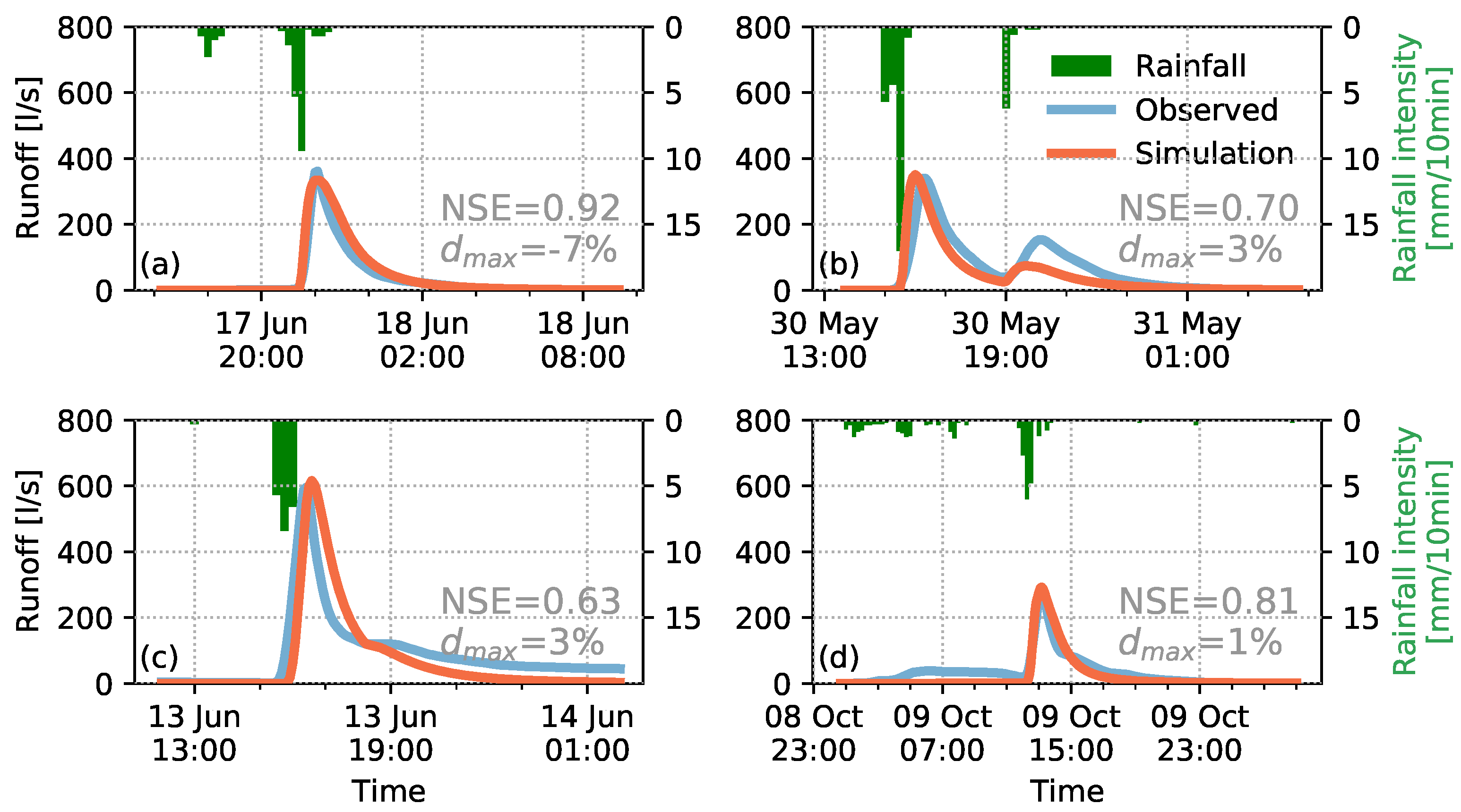
Having demonstrated the high predictive skill in interception modeling, Figure 4 shows the model results of the runoff calibration, which focus on runoff generation processes below the canopy (i.e., infiltration and surface runoff). The parameters found through minimizing the objective function f in Equation (5) using SCE-UA in spotpy yield the following parameters with convergence after 573 iterations:
- Parameter b of the Brooks-Corey retention curve: 13.1876;
- Scaling factor for Manning’s n roughness: 3.57788;
- Scaling factor for saturated hydraulic conductivity : 0.0700464.
The scaling parameters found through calibration deviate from 1.0, suggesting that the assignment of land-use classes to roughness and conductivity values has been altered during calibration. The resulting values are still viewed meaningful. However, they are effective values that include sub-scale variability [45], like, e.g., unknown soil variability and local compaction or obstacles on the surface.
The range of Nash–Sutcliffe model efficiency E values obtained for all events extends from 0.63 to 0.92. In the process of model calibration, E amounts to 0.92 (event 1) and 0.70 (event 2), respectively. The goodness-of-fit achieved for event 1 (E = 0.92) is considered to be very good, while for event 2, E = 0.70 is still satisfactory. One possible reason for the lower model skill achieved for event 2 could be the fact that the event consists of two peaks. However, given the good match of peak flow values, the results of the calibration are acceptable.
The validation confirms that the model calibration is transferable to other events. Even though the Nash–Sutcliffe model efficiency found for event 3 (E = 0.63) is lower than the corresponding values found during calibration, it is still within an acceptable range of values higher than 0.5 [46] (it is worth mentioning that even a model with E > 0 has a higher predictive value than predicting just the average value, which is the benchmark value included in E). Event 4 even reflects a better model skill with E = 0.81. Similar to the calibration events, peak discharge is represented well even for the events considered for validating the model. For both types of events, i.e., calibration and validation, the differences in peak runoff are within the range ±3% (except for event 1, for which the difference amounts to 7%), which we view as a very good coincidence. Hence, we assume that the model is successfully calibrated and validated according to the split-sample test and that it has predictive skill for events not considered in the calibration procedure.
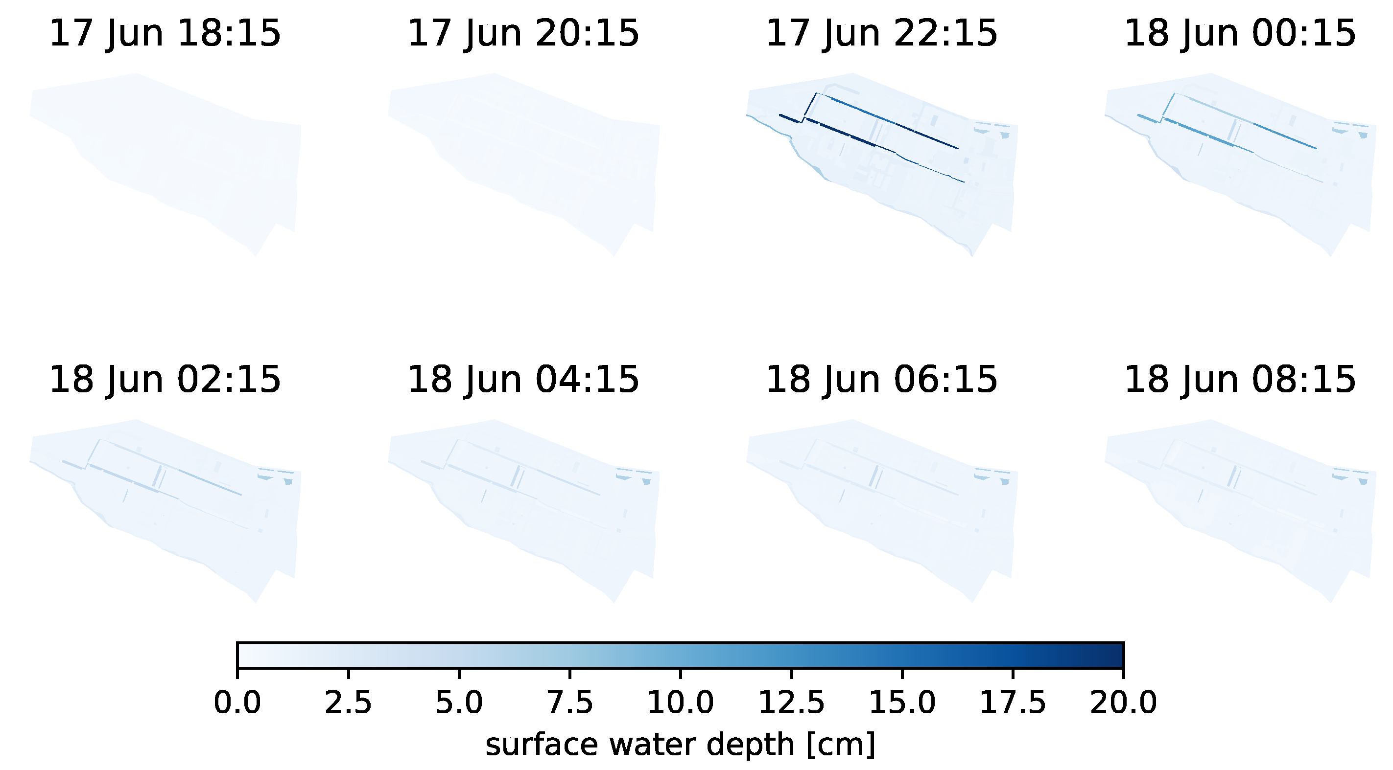
Figure 5 compiles a series of maps that show the spatio-temporal distribution of surface water in the study area. This visualization helps to analyze whether the model is also realistic in terms of runoff routing on the surface. In contrast to other models that utilize a unit-hydrograph or similar parametrizations to compute runoff concentration, explicit kinematic surface water routing is used instead. The temporal evolution of maps highlights how water is routed via the swales from east to west towards the intake structure (for which runoff measurements exist). Since no water level observations are available for the events, this figure is at least helpful for checking whether the model shows a realistic surface routing. The sequence of maps suggests that the model reflects a plausible surface routing.
3.3. The Role of Trees in Pluvial Flooding
Finally, the role of trees in runoff generation is analyzed through comparing the runs from Figure 4 with corresponding runs, which have been conducted without trees. Table 5 compiles the most important characteristics for each of these event-based comparisons. For each event, the deactivation of trees is quantified in terms of (i) increase in maximum runoff, (ii) the increase in volume and (iii) its relative change, for both.
The differences in peak discharge at the quarter scale range between 17% and 27% and, therefore, exceed the differences between observed and modeled peak runoff for all events. Predicted changes in peak runoff associated to changes in tree coverage therefore clearly exceed the inaccuracy in predicting model discharge by one order of magnitude. The values are highest for events 2 (27%) and 1 (25%), while they are lower but still in the order of 15–20% for events 3 and 4. Likewise, the changes in volume reach up to 18% for event 2 if trees are not included. Similar values are reached for event 1 and 4 (15%), and for event 3 (11%). These rates of change demonstrate that the coverage of trees, though no dominant land use fraction, is important to retain water during heavy rainfall events.
The average tree-scale values are remarkable: Peak runoff is reduced by 0.139 ± 0.033 L/s for all events. Even though the corresponding relative contribution in reducing peak runoff is small (∼0.04%), the average value of 0.139 ± 0.033 L/s is still a tangible result. In terms of volume, the relative contribution for each tree is also small (∼0.02%). However, the average difference in volume computed for each tree (631 ± 73 L) is higher than the value one might expect from just considering maximum interception capacity: the average projected area of an average tree amounts to 43.95 m. Given an interception capacity of ∼10 mm yields 439.5 L of intercepted water for each tree (439.5 L·611 = 268,535 L for all 611 trees). This volume is only ∼70% of the volume differences achieved from comparison of the modeling experiments. A reason for this higher retention could be attributed to the non-linearity in the model. Intercepted water does not contribute to infiltration and surface runoff, respectively. However, in case of absent trees more water will turn into surface runoff that even affects areas downhill from the considered area without trees. More surface runoff in downstream areas, which are laterally connected, even potentially exceeds the infiltration capacity. This is especially true during peak rainfall intensities, which, in turn, highlights the relevance of trees.
Indeed, the percentage described here depends on the rainfall event in terms of magnitude. Hence, the relative contribution is lower for higher rainfall intensities. This is especially relevant, since it is expected that climate change might lead to increasing rainfall intensities. The return periods considered here do not represent extreme values, but they are typical values considered in urban drainage planning and associated guidelines (e.g., DIN EN 752 (DIN EN 752:2017-07 Drain and sewer systems outside buildings—Sewer system management)). Thus, our findings highlight that each tree contributes to reduce peak discharge in an quantifiable way, whilst being tangible for stakeholders.
3.4. Limitations
The accuracy of hydrological model outputs highly depends on the rainfall data. A major uncertainty in modeling hydrological response in urban areas is related to spatio-temporal rainfall variability [47]. Rainfall variability occurs below 1 km and therefore can not be resolved by operational radar networks. For modeling fast responding catchments, a higher density of rain gauges is required [48,49]. Furthermore, no information about the initial soil saturation is available that can be taken into account. However, we can make assumptions based on the precipitation conditions of the previous days.
Urban soils are highly heterogeneous, due to compaction, sealing and other anthropogenic impacts, where there is a lack of data on their spatial distribution. Additionally, the used soil dataset in this study is limited on spatial variability, and therefore probably does not represent reality in accurate detail. Furthermore, we used a simple one layer approach, which might simplify the infiltration processes. Due to disturbed compacted soils and porosity reduction in urban areas, infiltration rates can be very low [50,51]. We reduced the given porosity according to literature (0.453 for sandy loam) [34] to 0.3. Even though we assume a porosity reduction due to urban soil compaction, we decided not to calibrate this parameter because of the availability of principle data from feasible literature. Other possible parameters that could be calibrated are further terms of the Brooks–Corey retention curve, such as the porosity decay or adjustments to the retention curve through the provision of value pairs of volumetric soil moisture and matrix potential, respectively [30]. Salvadore et al. [8] also suggest new techniques in calibration that are not only based on curve fitting at single locations, but also spatial distributed indices.
Likewise, uncertainties in the measurement should not be disregarded as a possible source of error since the urban hydrology system is highly complex with lots of uncertainties and not yet completely understood [8]. For instance, in Vauban the throughfall is measured with a tipping bucket rain gauge. Compared to standard rainfall measurements, throughfall measured this way is subject to higher maintenance (regular removal of leafs and needles), which needs to be considered as additional uncertainty in calculating interception with a simple bucket model. Errors in modeling and measurements are both possible. Especially for urban hydrology, data availability is limited and more measurements and open datasets (e.g., the Bellinge dataset [52]) are needed for calibrating models [8,53]. Besides level and runoff data, also more measurements of interception and infiltration should be collected to improve the urban hydrology system and thus modeling in this field.
4. Conclusions and Outlook
With respect to the two research questions raised in this paper, the major findings can be summarized as follows: The results suggest that our modeling approach is capable of representing both interception and surface runoff in a single model structure with a sufficient level of detail. This has been demonstrated by a good correspondence of modeled and measured runoff data and interception, respectively. Moreover, the model is able to quantify the contribution of single trees to mitigate effects of pluvial flooding at the quarter scale, at least on average.
The single contribution of each tree to reduce the flood peak (i.e., 0.139 ± 0.033 L/s) is site-specific, as it depends upon area size and tree coverage. Thus, the reduction in peak discharge cannot be transferred from one site to another. Whereas, the modeling approach can enable a transfer to other sites, since the comparison of observed and modeled interception and runoff, respectively, underlines a skillful representation runoff generation processes. At least, re-calibrating soil parameters is recommended if data is available. However, the site-specific single contribution of each tree is viewed as a tangible value, one that approximately corresponds to retaining a volume corresponding to one cup of coffee per second. This value could be computed likewise for arbitrary study areas with the approach described in this paper and communicated to stakeholders to make them aware of the role of trees in general and that every single tree is significant in flood mitigation at the quarter scale. Since the model is viewed scenario-capable, different levels of tree coverage or higher rainfall intensities could be studied likewise with LEAFlood. Furthermore, urban trees can store a greater amount of water in comparison to natural forest trees, since they tend to have a more circumference growth and thus a greater potential of water storage capacity [54]. With this outcome, new approaches in the assessment of flood regulating ecosystem services for heavy rainfall events in urban areas can be developed.
Unlike other hydrological models and studies that recommend a resolution of 3 to 5 m for an adequate representation of the urban structure [55], the one used here is based on irregular polygons. Comparisons with a raster approach have shown no improvement in the results, therefore a triangle or raster approach is not necessary. This significantly reduces the computation time and features the preparation of the modeling domain with standard GIS tools. The programming based structure of CMF provides the possibility to couple the hydrological model with other models [56] to include dynamic interactions with surrounding environments of climate, land use, ecosystems and society. LEAFlood is ready to be adopted for other research questions. For instance, the evapotranspiration could be included for longer or intermittent rainfall events. This can be an important tool for informing decision makers and urban planners in the future, in order to understand and evaluate systems holistically.
Author Contributions
K.S.M.C.: Data preparation, modeling, testing; T.W.: study design, model development; K.F.: study design, auto-calibration, supervision. All authors contributed to writing and have read and agreed to the published version of the manuscript.
Funding
This research received no external funding.
Institutional Review Board Statement
Not applicable.
Informed Consent Statement
Not applicable.
Data Availability Statement
The meteorological data are freely available from the DWD Climate Data Center (https://opendata.dwd.de/climate_environment/, accessed on 25 March 2022). The LEAFlood model code is open source software (https://0-doi-org.brum.beds.ac.uk/10.5281/zenodo.6594181, accessed on 30 May 2022).
Acknowledgments
The authors would like to thank Markus Weiler and Hannes Leistert from the University of Freiburg for providing the spatial data and measurements for calibration. The work would not have been possible without these data. Many thanks to Philipp Kraft for technical support with model questions and to Luisa-Bianca Thiele for discussions on model calibration. Furthermore, our thanks go to Bora Shehu for providing the most recent rainfall statistics for the study area. We would also like to thank Laurens Bouwer, Torsten Weber and Steffen Bender for the internal review, Ludwig Lierhammer and Lars Buntemeyer for the code review as well as Angie Faust for language proofreading.
Conflicts of Interest
The authors declare no conflict of interest.
References
- Melsen, L. It Takes a Village to Run a Model—The Social Practices of Hydrological Modeling. Water Resour. Res. 2022, 58, e2021WR030600. [Google Scholar] [CrossRef]
- Asadian, Y.; Weiler, M. A new approach in measuring rainfall interception by urban trees in coastal British Columbia. Water Qual. Res. J. 2009, 44, 16–25. [Google Scholar] [CrossRef]
- Coville, R.; Endreny, T.; Nowak, D.J. Modeling the Impact of Urban Trees on Hydrology. In Forest-Water Interactions; Levia, D.F., Carlyle-Moses, D.E., Iida, S., Michalzik, B., Nanko, K., Tischer, A., Eds.; Series Title: Ecological Studies; Springer International Publishing: Cham, Switzerland, 2020; Volume 240, pp. 459–487. [Google Scholar] [CrossRef]
- Downer, C.W.; Ogden, F.L.; Martin, W.D.; Harmon, R.S. Theory, development, and applicability of the surface water hydrologic model CASC2D. Hydrol. Process. 2002, 16, 255–275. [Google Scholar] [CrossRef]
- Mitasova, H.; Thaxton, C.; Hofierka, J.; McLaughlin, R.; Moore, A.; Mitas, L. Path sampling method for modeling overland water flow, sediment transport, and short term terrain evolution in Open Source GIS. Dev. Water Sci. 2004, 55, 1479–1490. [Google Scholar] [CrossRef]
- Tyrna, B.; Assmann, A.; Fritsch, K.; Johann, G. Large-scale high-resolution pluvial flood hazard mapping using the raster-based hydrodynamic two-dimensional model FloodAreaHPC: Large-scale high-resolution pluvial flood hazard mapping. J. Flood Risk Manag. 2018, 11, S1024–S1037. [Google Scholar] [CrossRef] [Green Version]
- Iffland, R.; Förster, K.; Westerholt, D.; Pesci, M.H.; Lösken, G. Robust Vegetation Parameterization for Green Roofs in the EPA Stormwater Management Model (SWMM). Hydrology 2021, 8, 12. [Google Scholar] [CrossRef]
- Salvadore, E.; Bronders, J.; Batelaan, O. Hydrological modelling of urbanized catchments: A review and future directions. J. Hydrol. 2015, 529, 62–81. [Google Scholar] [CrossRef]
- Cuo, L.; Lettenmaier, D.P.; Alberti, M.; Richey, J.E. Effects of a century of land cover and climate change on the hydrology of the Puget Sound basin. Hydrol. Process. 2009, 23, 907–933. [Google Scholar] [CrossRef]
- Dwarakish, G.; Ganasri, B. Impact of land use change on hydrological systems: A review of current modeling approaches. Cogent Geosci. 2015, 1, 1115691. [Google Scholar] [CrossRef]
- Strasser, U.; Förster, K.; Formayer, H.; Hofmeister, F.; Marke, T.; Meißl, G.; Nadeem, I.; Stotten, R.; Schermer, M. Storylines of combined future land use and climate scenarios and their hydrological impacts in an Alpine catchment (Brixental/Austria). Sci. Total Environ. 2019, 657, 746–763. [Google Scholar] [CrossRef]
- Wagner, P.D.; Bhallamudi, S.M.; Narasimhan, B.; Kumar, S.; Fohrer, N.; Fiener, P. Comparing the effects of dynamic versus static representations of land use change in hydrologic impact assessments. Environ. Model. Softw. 2019, 122, 103987. [Google Scholar] [CrossRef]
- Addor, N.; Melsen, L.A. Legacy, Rather than Adequacy, Drives the Selection of Hydrological Models. Water Resour. Res. 2019, 5, 378–390. [Google Scholar] [CrossRef] [Green Version]
- Kraft, P.; Vaché, K.B.; Frede, H.G.; Breuer, L. CMF: A Hydrological Programming Language Extension For Integrated Catchment Models. Environ. Model. Softw. 2011, 26, 828–830. [Google Scholar] [CrossRef]
- Förster, K.; Westerholt, D.; Kraft, P.; Lösken, G. Unprecedented Retention Capabilities of Extensive Green Roofs—New Design Approaches and an Open-Source Model. Front. Water 2021, 3, 122. [Google Scholar] [CrossRef]
- Krebs, G.; Kokkonen, T.; Valtanen, M.; Setälä, H.; Koivusalo, H. Spatial resolution considerations for urban hydrological modelling. J. Hydrol. 2014, 512, 482–497. [Google Scholar] [CrossRef]
- Jackisch, N.; Brendt, T.; Weiler, M.; Lange, J. Evaluierung der Regenwasserbewirtschaftung im Vaubangelände, Freiburg i.Br; Technical Report. 2013. Available online: http://www.hydrology.uni-freiburg.de/forsch/regenwasservauban/Regenwasserprojekt_Vauban_Endbericht_Final.pdf (accessed on 15 June 2022).
- Jackisch, N.; Weiler, M. The hydrologic outcome of a Low Impact Development (LID) site including superposition with streamflow peaks. Urban Water J. 2017, 14, 143–159. [Google Scholar] [CrossRef]
- Steinbrich, A.; Henrichs, M.; Leistert, H.; Scherer, I.; Schuetz, T.; Uhl, M.; Weiler, M. Ermittlung eines naturnahen Wasserhaushalts als Planungsziel für Siedlungen (Determination of a natural water balance as reference for planning in urban areas). Hydrol. Und Wasserbewirtsch. 2018, 62, 400–409. [Google Scholar] [CrossRef]
- DWD Climate Data Center (CDC): Multi-Annual Station Means for the Climate Normal Reference Period 1981–2010, for Current Station Location and for Reference Station Location. Version V0.x. 2022. Available online: https://opendata.dwd.de/climate_environment/CDC/observations_germany/climate/multi_annual/mean_81-10/ (accessed on 12 March 2022).
- Leistert, H.; Steinbrich, A.; Schütz, T.; Weiler, M. Wie kann die hydrologische Komplexität von Städten hinreichend in einem Wasserhaushaltsmodell abgebildet werden? In M3—Messen, Modellieren, Managen in Hydrologie und Wasserressourcenbewirtschaftung. Beiträge zum Tag der Hydrologie am 22./23. März 2018 an der Technischen Universität Dresden. Tag der Hydrologie; Technischen Universität Dresden: Dresden, Germany, 2018; pp. 227–236. [Google Scholar]
- Steinbrich, A.; Leistert, H.; Weiler, M. Model-based quantification of runoff generation processes at high spatial and temporal resolution. Environ. Earth Sci. 2016, 75, 1423. [Google Scholar] [CrossRef]
- Fletcher, T.D.; Shuster, W.; Hunt, W.F.; Ashley, R.; Butler, D.; Arthur, S.; Trowsdale, S.; Barraud, S.; Semadeni-Davies, A.; Bertrand-Krajewski, J.L.; et al. SUDS, LID, BMPs, WSUD and more—The evolution and application of terminology surrounding urban drainage. Urban Water J. 2015, 12, 525–542. [Google Scholar] [CrossRef]
- van Hattum, T.; Blauw, M.; Jensen, M.B.; de Bruin, K. Towards Water Smart Cities: Climate Adaptation Is a Huge Opportunity to Improve the Quality of Life in Cities; Technical Report; Wageningen University & Research: Wageningen, The Netherlands, 2016. [Google Scholar]
- Coates, G.J. The sustainable urban district of Vauban in Freiburg, Germany. Int. J. Des. Nat. Ecodyn. 2013, 8, 265–286. [Google Scholar] [CrossRef] [Green Version]
- DWD Climate Data Center (CDC): Historical 10-Minute Station Observations of Pressure, Air Temperature (at 5 cm and 2 m Height), Humidity and Dew Point for Germany. Version V1. 2019. Available online: https://opendata.dwd.de/climate_environment/CDC/observations_germany/climate/10_minutes/air_temperature/ (accessed on 9 July 2021).
- DWD Climate Data Center (CDC): Historical 10-Minute Station Observations of Solar Incoming Radiation, Longwave Downward Radiation and Sunshine Duration for Germany. Version V1. 2022. Available online: https://opendata.dwd.de/climate_environment/CDC/observations_germany/climate/10_minutes/solar/ (accessed on 9 July 2021).
- DWD Climate Data Center (CDC): Historical 10-Minute Station Observations of Mean Wind Speed and Wind Direction for Germany. Version V1. 2019. Available online: https://opendata.dwd.de/climate_environment/CDC/observations_germany/climate/10_minutes/wind/ (accessed on 9 July 2021).
- Wübbelmann, T.; Förster, K. Landscape and vEgetAtion-Dependent Flood Model (LEAFlood). Available online: https://0-doi-org.brum.beds.ac.uk/10.5281/zenodo.6594181 (accessed on 30 May 2022). [CrossRef]
- Kraft, P. cmf Documentation. Available online: https://philippkraft.github.io/cmf/index.html (accessed on 23 March 2022).
- Clark, M.; Kavetski, D.; Fenicia, F. Pursuing the method of multiple working hypotheses for hydrological modeling: Hypothesis testing in hydrology. Water Resour. Res. 2011, 47, 1–16. [Google Scholar] [CrossRef] [Green Version]
- Schulla, J. Model Description WaSiM (Water Balance Simulation Model)—Completely Revised Version of 2012 with 2013 to 2015 Extensions; Hydrology Software Consulting J. Schulla: Zurich, Switzerland, 2015. [Google Scholar]
- Rutter, A.; Kershaw, K.; Robins, P.; Morton, A. A predictive model of rainfall interception in forests, 1. Derivation of the model from observations in a plantation of Corsican pine. Agric. Meteorol. 1971, 9, 367–384. [Google Scholar] [CrossRef]
- Kartieranleitung, B. Ad-hoc-AG Boden. Bodenkdundliche Kartieranleitung Hann. 2005, 5, 438. [Google Scholar]
- Gregory, J.H.; Dukes, M.D.; Jones, P.H.; Miller, G.L. Effect of urban soil compaction on infiltration rate. J. Soil Water Conserv. 2006, 61, 117–124. [Google Scholar]
- Refsgaard, J.C. Terminology, Modelling Protocol and Classification of Hydrological Model Codes. In Distributed Hydrological Modelling; Abbott, M.B., Refsgaard, J.C., Eds.; Water Science and Technology Library; Kluwer Academic Publishers: Dordrecht, The Netherlands, 1996; Volume 22, pp. 17–39. [Google Scholar]
- Klemes, V. Operational testing of hydrological simulation models. Hydrolog. Sci. J. 1986, 31, 13–24. [Google Scholar] [CrossRef]
- Shehu, B.; Willems, W.; Stockel, H.; Thiele, L.; Haberlandt, U. Regionalisation of Rainfall Depth-Duration-Frequency curves in Germany. Hydrol. Earth Syst. Sci. Discuss. 2022, preprint. [Google Scholar] [CrossRef]
- Förster, K.; Garvelmann, J.; Meißl, G.; Strasser, U. Modelling forest snow processes with a new version of WaSiM. Hydrol. Sci. J. 2018, 63, 1540–1557. [Google Scholar] [CrossRef] [Green Version]
- Hall, M.J. How well does your model fit the data? J. Hydroinform. 2001, 3, 49–55. [Google Scholar] [CrossRef] [Green Version]
- Duan, Q.; Sorooshian, S.; Gupta, V.K. Optimal use of the SCE-UA global optimization method for calibrating watershed models. J. Hydrol. 1994, 158, 265–284. [Google Scholar] [CrossRef]
- Houska, T.; Kraft, P.; Chamorro-Chavez, A.; Breuer, L. SPOTting Model Parameters Using a Ready-Made Python Package. PLoS ONE 2015, 10, e0145180. [Google Scholar] [CrossRef]
- Alves, P.L.; Formiga, K.T.M.; Traldi, M.A.B. Rainfall interception capacity of tree species used in urban afforestation. Urban Ecosyst. 2018, 21, 697–706. [Google Scholar] [CrossRef]
- Förster, K.; Gelleszun, M.; Meon, G. A weather dependent approach to estimate the annual course of vegetation parameters for water balance simulations on the meso- and macroscale. Adv. Geosci. 2012, 32, 15–21. [Google Scholar] [CrossRef] [Green Version]
- Kirchner, J.W. Getting the right answers for the right reasons: Linking measurements, analyses, and models to advance the science of hydrology. Water Resour. Res. 2006, 42, W03S04. [Google Scholar] [CrossRef]
- Moriasi, D.N.; Arnold, J.G.; van Liew, M.W.; Bingner, R.L.; Harmel, R.D.; Veith, T.L. Model evaluation guidelines for systematic quantification of accuracy in watershed simulations. Trans. ASABE 2007, 50, 885–900. [Google Scholar] [CrossRef]
- Cristiano, E.; ten Veldhuis, M.c.; Van De Giesen, N. Spatial and temporal variability of rainfall and their effects on hydrological response in urban areas–a review. Hydrol. Earth Syst. Sci. 2017, 21, 3859–3878. [Google Scholar] [CrossRef] [Green Version]
- Gires, A.; Tchiguirinskaia, I.; Schertzer, D.; Schellart, A.; Berne, A.; Lovejoy, S. Influence of small scale rainfall variability on standard comparison tools between radar and rain gauge data. Atmos. Res. 2014, 138, 125–138. [Google Scholar] [CrossRef] [Green Version]
- Jensen, N.; Pedersen, L. Spatial variability of rainfall: Variations within a single radar pixel. Atmos. Res. 2005, 77, 269–277. [Google Scholar] [CrossRef]
- Pitt, R.; Lantrip, J.; O’Connor, T.P. Infiltration through disturbed urban soils. J. Water Manag. Model. 2000, 1–22. [Google Scholar] [CrossRef]
- Markovi, G.; Zele, M.; Káposztásová, D.; Hudáková, G. Rainwater infiltration in the urban areas. WIT Trans. Ecol. Environ. 2014, 181, 313–320. [Google Scholar]
- Pedersen, A.N.; Pedersen, J.W.; Vigueras-Rodriguez, A.; Brink-Kjær, A.; Borup, M.; Mikkelsen, P.S. The Bellinge data set: Open data and models for community-wide urban drainage systems research. Earth Syst. Sci. Data 2021, 13, 4779–4798. [Google Scholar] [CrossRef]
- Fletcher, T.D.; Andrieu, H.; Hamel, P. Understanding, management and modelling of urban hydrology and its consequences for receiving waters: A state of the art. Adv. Water Resour. 2013, 51, 261–279. [Google Scholar] [CrossRef]
- Carlyle-Moses, D.E.; Livesley, S.; Baptista, M.D.; Thom, J.; Szota, C. Urban Trees as Green Infrastructure for Stormwater Mitigation and Use. In Forest-Water Interactions; Levia, D.F., Carlyle-Moses, D.E., Iida, S., Michalzik, B., Nanko, K., Tischer, A., Eds.; Series Title: Ecological Studies; Springer International Publishing: Cham, Switzerland, 2020; Volume 240, pp. 397–432. [Google Scholar] [CrossRef]
- Cotton, G.K.; Strasser, H. High Resolution Urban Hydrologic Modeling. In Proceedings of the World Environmental and Water Resources Congress 2012: Crossing Boundaries, Albuquerque, NM, USA, 20–24 May 2012; pp. 1889–1898. [Google Scholar]
- Kraft, P.; Multsch, S.; Vaché, K.; Frede, H.G.; Breuer, L. Using Python as a coupling platform for integrated catchment models. Adv. Geosci. 2010, 27, 51–56. [Google Scholar] [CrossRef] [Green Version]
Figure 1.
Land use and location of the study area Vauban.

Figure 2.
Used processes and defining parameters of storages in CMF.

Figure 3.
Comparison of observed and predicted interception load for (a) event #1 (June 2011), (b) event #2 (May 2012), and (c) event #3 (June 2012)).
Figure 3.
Comparison of observed and predicted interception load for (a) event #1 (June 2011), (b) event #2 (May 2012), and (c) event #3 (June 2012)).

Figure 4.
Results of calibration and validation for (a) event #1 (June 2011), (b) event #2 (May 2012), (c) event #3 (June 2012), and (d) event #4 (October 2012). Nash–Sutcliffe model efficiency E (NSE) and the difference between observed and predicted peak runoff (as percentage) are indicated for each event.

Figure 5.
Spatial distribution of surface water depth for different time steps of event #1 (June 2011). Maximum runoff occurs around 22:15.
Figure 5.
Spatial distribution of surface water depth for different time steps of event #1 (June 2011). Maximum runoff occurs around 22:15.


Table 1.
Overview of the input datasets for the LEAFlood model.
| Data | Type | Resolution | Units | Geodata | Climate Data | Measured | Source |
|---|---|---|---|---|---|---|---|
| DEM | Raster | 1 m | m | x | Freiburg University | ||
| Throughfall | Timeseries | 1 min | mm/min | x | Freiburg University | ||
| Land use map | Shapefile | - | - | x | Freiburg University | ||
| Precipitation | Timeseries | 1 min | mm/min | x | Freiburg University | ||
| Relative humidity | Timeseries | 5 min | % | x | Freiburg station [26] | ||
| Runoff | Timeseries | 5 min | L/s | x | Freiburg University | ||
| Soil class map | Shapefile | - | - | x | Freiburg University | ||
| Sunshine hours | Timeseries | 5 min | h/h | x | Freiburg station [27] | ||
| Temperature | Timeseries | 5 min | C | x | Freiburg station [26] | ||
| Tree coverage | Shapefile | - | - | x | Freiburg University | ||
| Tree number | Aerial image | unit | trees | x | Google Earth | ||
| Wind speed | Timeseries | 5 min | m/s | x | Freiburg station [28] |
Table 2.
Setting and processes in cmf.
| Process/ Parameter | Setting |
|---|---|
| Interception | Rutter Interception |
| Throughfall | |
| Canopy Overflow | |
| Infiltration | Green Ampt |
| Brooks Corey Retention curve | |
| Layer depth | 0.5 m |
| Saturated Conductivity () | 0.3 m/d (base value) |
| Porosity | 0.3 |
| Surface Runoff | Kinematic |
Table 3.
The roughness coefficient Manning’s n and the saturated conductivity () defined for each land use class.
Table 3.
The roughness coefficient Manning’s n and the saturated conductivity () defined for each land use class.
| Land Use | Manning’s n | Saturated Conductivity [m/Day] |
|---|---|---|
| Urban Sealed Area | 0.013 | 0 |
| Green Area | 0.03 | 0.25 |
| Green Roofs | 0.03 | 0.72 |
| Vegetative Swale | 0.03 | 0.7 |
| Water | 0.03 | 0.015 |
Table 4.
Overview of events with highest peak runoff in the runoff time series, covering the years 2011–2012. ‘Saturated depth’ is the initial condition guess used for each event, while the last column (‘c/v’) indicates whether the event is used for calibration (c) or validation (v).
Table 4.
Overview of events with highest peak runoff in the runoff time series, covering the years 2011–2012. ‘Saturated depth’ is the initial condition guess used for each event, while the last column (‘c/v’) indicates whether the event is used for calibration (c) or validation (v).
| Event | Start Date | Time | Duration [h] | Peak Intensity [mm/h] | Return Period [a] | Rainfall Event [mm] | Total −10 d [mm] | Peak Runoff [L/s] | Saturated Depth [m] | c/v |
|---|---|---|---|---|---|---|---|---|---|---|
| #1 | 17 June 2011 | 16:15 | 17 | 16.5 | <1 | 23.4 | 41.6 | 361 | 0.50 | c |
| #2 | 30 May 2012 | 13:40 | 15 | 27.9 | ∼5 | 35.3 | 35.3 | 339 | 20.0 | c |
| #3 | 13 June 2012 | 12:00 | 19 | 25.1 | 1–5 | 27.4 | 82.9 | 595 | 0.25 | v |
| #4 | 9 October 2012 | 00:40 | 28 | 14.2 | <1 | 32.7 | 15.4 | 291 | 7.00 | v |
Table 5.
Results of the model experiments considering runs with and without trees. The values indicate the increase in peak runoff and volume if trees are not included in the simulation.
Table 5.
Results of the model experiments considering runs with and without trees. The values indicate the increase in peak runoff and volume if trees are not included in the simulation.
| Event | Quarter Scale | Tree Scale (Avg.) | ||||||
|---|---|---|---|---|---|---|---|---|
| [L/s] | [%] | Volume [L] | Volume [%] | [L/s] | [%] | Volume [L] | Volume [%] | |
| #1 | 83 | 25% | 368,550 | 15% | 0.135 | 0.04% | 603 | 0.02% |
| #2 | 96 | 27% | 432,141 | 18% | 0.156 | 0.04% | 707 | 0.03% |
| #3 | 104 | 17% | 409,373 | 11% | 0.170 | 0.04% | 670 | 0.02% |
| #4 | 57 | 19% | 332,064 | 15% | 0.093 | 0.03% | 543 | 0.02% |
Publisher’s Note: MDPI stays neutral with regard to jurisdictional claims in published maps and institutional affiliations. |
© 2022 by the authors. Licensee MDPI, Basel, Switzerland. This article is an open access article distributed under the terms and conditions of the Creative Commons Attribution (CC BY) license (https://creativecommons.org/licenses/by/4.0/).
Share and Cite
MDPI and ACS Style
Medina Camarena, K.S.; Wübbelmann, T.; Förster, K. What Is the Contribution of Urban Trees to Mitigate Pluvial Flooding? Hydrology 2022, 9, 108. https://0-doi-org.brum.beds.ac.uk/10.3390/hydrology9060108
AMA Style
Medina Camarena KS, Wübbelmann T, Förster K. What Is the Contribution of Urban Trees to Mitigate Pluvial Flooding? Hydrology. 2022; 9(6):108. https://0-doi-org.brum.beds.ac.uk/10.3390/hydrology9060108
Chicago/Turabian StyleMedina Camarena, Karina Sinaí, Thea Wübbelmann, and Kristian Förster. 2022. "What Is the Contribution of Urban Trees to Mitigate Pluvial Flooding?" Hydrology 9, no. 6: 108. https://0-doi-org.brum.beds.ac.uk/10.3390/hydrology9060108
Note that from the first issue of 2016, this journal uses article numbers instead of page numbers. See further details here.