
Importance of Flood Samples for Estimating Sediment and Nutrient Loads in Mediterranean Rivers

1
HYDRIAD Eau et Environnement, 443 Rte St-Genies, 30730 Saint-Bauzély, France
2
Hydro-Geology Department, Avignon Université, UMR 1114 EMMAH (AU/INRAE), 301 rue Baruch de Spinoza, BP 21239, CEDEX 09, 84911 Avignon, France
3
Agence de l’Eau Rhône Méditerranée Corse, 2-4 allée de Lodz, CEDEX 07, 69363 Lyon, France
*
Authors to whom correspondence should be addressed.
Hydrology 2022, 9(6), 110; https://0-doi-org.brum.beds.ac.uk/10.3390/hydrology9060110
Submission received: 18 May 2022
/
Revised: 12 June 2022
/
Accepted: 15 June 2022
/
Published: 16 June 2022
Abstract
:Protecting the quality of coastal water bodies requires the assessment of contaminant discharge brought by rivers. Numerous methods have been proposed for calculating sediment and nutrient loads. The most widely used and generally recommended are the flow-weighted mean concentration method (FWMC) and the flow duration rating curve method (FDRC). In the Mediterranean basin, the hydrology is characterized by infrequent but very intense rainfall events. The flows taking place during these periods last only a few hours to a few days but can represent the largest part of the annual flow. The loads associated with these events can also account for most of the annual load. A reinforced water-quality monitoring program (especially during floods) was carried out for five years (August 2015–July 2020) on six tributaries of French Mediterranean lagoons. The loads calculated by FWMC and FDRC methods were very different. Total suspended solid loads calculated by FWMC were on average 5.0 times higher than those calculated by FDRC. Similarly, total phosphorus loads were 3.5 times higher and total nitrogen loads were 1.6 times higher. The results show that too many flood samples can lead to considerable overestimation of particulate loads calculated by the FWMC method. Dissolved nutrients, on the other hand, are much less subject to overestimation.
1. Introduction
Protecting the quality of coastal water bodies (lagoons, mangroves, seas and oceans) requires the assessment of contaminant discharge brought by coastal rivers. The importance of the suspended or dissolved matter load depends on the concentration and water discharges over time. This involves measuring stream flow rates and associated concentrations over a long period of time. While discharge is often measured in a continuous manner, concentrations are only measured from time to time, usually at much lower frequencies than flow. Consequently, the load estimation may be difficult, and various techniques have been developed for this purpose [1].
For coastal rivers, the quantification of nutrient inputs is also complicated by the mixing that can occur at the interface between the river and the coastal water body. In [2], the importance of dispersion and turbulence in these mixing dynamics is discussed, showing the necessity for robust and frequent sampling to determine water-quality parameters. In addition, data scarcity can be considered as the main limitation for quantifying the nutrient behavior. In [3], a straightforward methodology is proposed to address the challenges associated with data quality and quantity problems for developing robust calculation tools.
According to [4], load estimation methods based on flow and concentration measurements can be divided into three broad categories: averaging, ratio and regression estimators. Averaging estimators are the simplest approach and have been extensively used. They combine the mean annual discharge calculated from instantaneous discharges and the mean concentration for the same period. The implicit assumptions are that the data are independent and identically distributed. Violations of these assumptions may lead to estimation bias, especially if the sampling does not cover the entire range of flow and concentration values [5].
Ratio estimators attempt to correct for the conditions at the time of sampling. For example, the load calculated by an averaging method can be corrected by the ratio of the long-term mean discharge to the mean discharge of samples. Ratio estimators classically use flow data as the auxiliary variable and load as the dependent variable. They assume a positive linear relationship between instantaneous loads and flows and the same for their variances [1].
Regression methods (or rating curves) use an empirical relationship between concentration and flow [6]. Generally, log–log regressions are used, because flow and concentration are assumed to be described by a bivariate lognormal distribution. The quality of the load estimate will depend on the representativeness of the relationship established and its validity over time. In [7], it was shown that accuracy of log–log regressions can be enhanced by using bias correction factors. The author in [8] improved the bias correction factor to yield a minimum variance unbiased estimator.
Many estimation methods exist, each with its advantages and disadvantages, strengths and weaknesses. None of these methods is perfect, and the choice of the method to be implemented must take into account not only the physical and hydrological characteristics of the watershed but also those of the monitoring program for flow and water quality. The selection of the appropriate method depends on the frequency and distribution of sampling, the variability in flow and the strength and form of the relationship between concentration and discharge, among other things [9].
For example, the flow-weighted mean concentration (FWMC) approach, classified as a regression method, was chosen for riverine load calculations for both suspended sediment and other compounds by the OSPAR convention in the RID program (Riverine Inputs and Direct Discharges) [10]. On the other hand, the flow duration rating curve method (FDRC), classified as a ratio estimator approach, is the method recommended by the FOEN (Swiss Federal Office for the Environment), following [11], where it was shown that it allows a better estimation of the annual discharge than other methods. These two methods are used in this paper and are described in the Section 2.
In the Mediterranean basin, the hydrology is characterized by infrequent but very intense rainfall events. The flows taking place during these periods last only a few hours to a few days but can represent the largest part of the annual water flow. The loads associated with these events can also account for most of the annual load. The Atlas of Riverine Inputs to the Mediterranean Sea for the period 1980–2010 was produced in 2015 by PERSEUS and UNEP/MAP [12]. According to this document, rivers are the main contributors to the input of nutrients to the sea, accounting for about 50% for nitrogen (N) and 75% for phosphorus (P). The report notes that the water discharge of rivers is highly dependent on climatic factors such as temperature and precipitation and on water uses such as irrigation and damming. Probably the most important criterion is related to the strong seasonal rainfall contrast between the summer and autumn–winter seasons.
This document shows that nitrate is, in most cases, the dominant nitrogen form, and its concentration covaries in space with other nitrogen compounds. In some rivers, the concentrations of ammonium may be unusually high compared to nitrate, which indicates strong wastewater emission close to the river mouth and a relatively low water discharge. Particulate phosphorus accounts for a high fraction of phosphorus fluxes in rivers, due to the strong affinity between orthophosphate (the major dissolved form of phosphorus) and particulates. At a global scale, dissolved phosphorus constitutes probably only about 10% of the phosphorus fluxes in rivers [13].
The Mediterranean region hosts around 400 coastal lagoons, covering a surface of over 6410 km2 [14]. Coastal lagoons are habitats declared as a priority by the European Union in the Habitats Directive, due to the biological communities that inhabit them [15]. Coastal lagoons are bodies of water with scarce renewal due to low freshwater inputs and reduced communication with the sea [16]. The problem of eutrophication is the most important impact reported in coastal lagoons, especially in those with inland water inputs and less exchange with the sea.
In France, numerous studies have been carried out on Mediterranean lagoons and the contaminants they receive. The French Rhone-Mediterranean and Corsica Water Agency has monitored the concentrations of pollutants transported by rivers for several decades. A reinforced water-quality monitoring program (especially during floods) was carried out for five hydrological years (August 2015–July 2020) on six tributaries of coastal lagoons. The objective was to characterize the temporal variability of the sediments and nutrients loads and, in particular, the role of floods in the estimation of the annual loads. Different methods of estimating loads were also tested, as well as their need or capacity to take into account the information obtained from flood periods and the impact of the lack of such knowledge.
This paper presents the results of the tests conducted for the comparison of the flow-weighted mean concentration (FWMC) method (that is, the method recommended in OSPAR studies) and the flow duration rating curves (FDRC) method (that is, the one recommended by the Swiss FOEN), with regard to the knowledge that is or is not available about the concentrations during flood events.
2. Materials and Methods
2.1. Studied Rivers
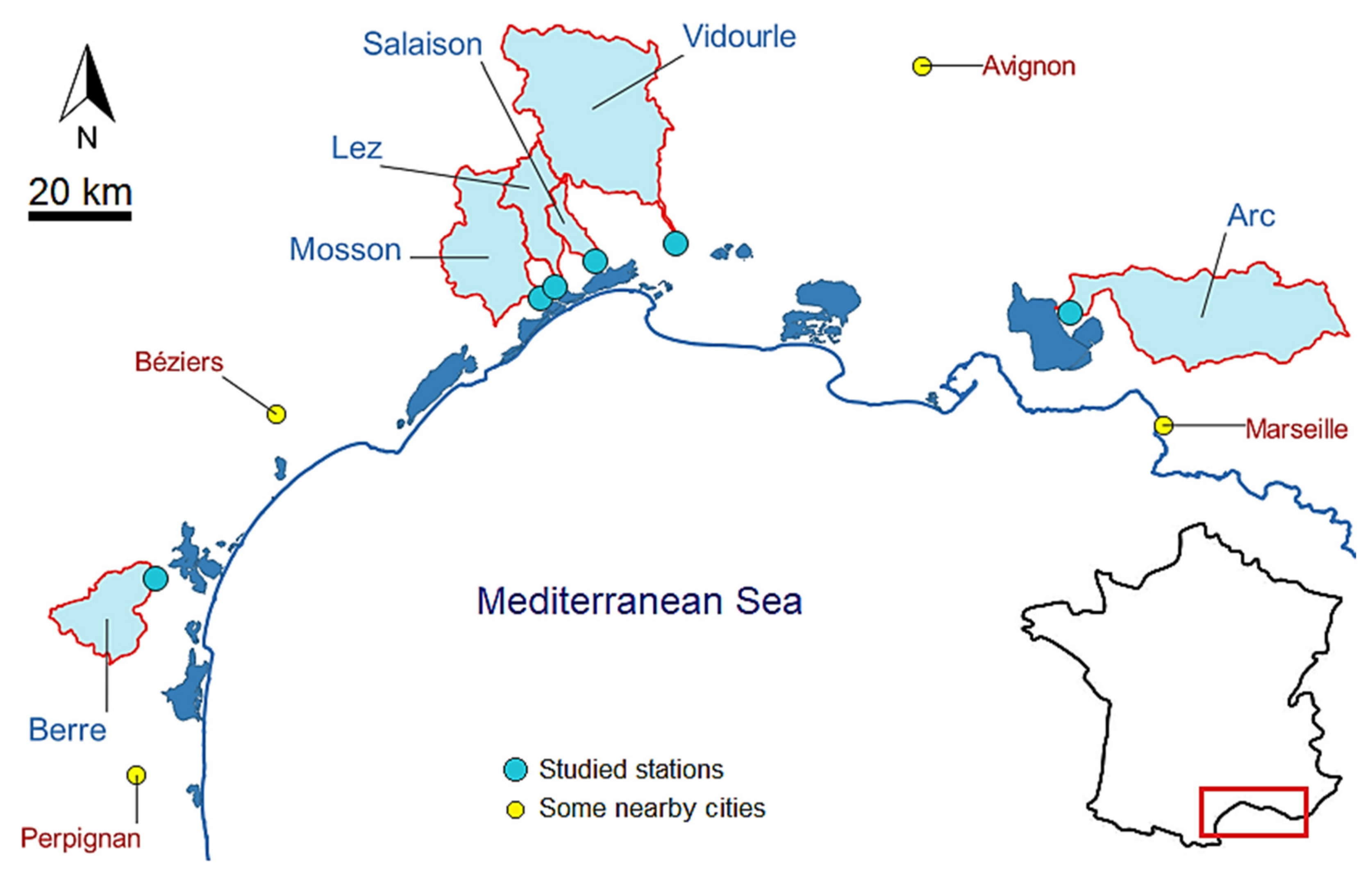
Six tributaries of French Mediterranean lagoons were studied. These were, from west to east: the Berre, Mosson, Lez, Salaison, Vidourle and Arc rivers (Figure 1). The six rivers have very different hydrological regimes and are influenced by very contrasting weather conditions. This is particularly the case for the four rivers located in the central zone, which are the ones most impacted by Mediterranean storm events (locally referred to as Cevennes episodes).
The six watersheds have very different physiographic and land use characteristics (Table 1). The watersheds range in size from 63.5 to 775 km2 and in average slope from 4.5% to 19.9%. The urban occupation (including commercial, artisanal and industrial zones) is very variable, ranging from 0.5% to 32.5%. Agriculture occupies between 26.3% and 48.7%, mainly represented by vineyards and cereals. From a geological point of view, their substrata are mainly made up of carbonate rocks (limestone and marl) dating from the Mesozoic (secondary era).
The Berre has a medium-sized watershed, with the highest average slope, the smallest population and a moderate agricultural occupation. The Mosson has a large watershed, with a fairly low average slope, a fairly large urban area, a moderate population and a moderate agricultural area. The Lez has a medium-sized watershed, with a fairly low average slope and a moderate agricultural occupation but the largest urban area and the largest population. The Salaison has the smallest watershed, with a very low slope, a moderate agricultural occupation, an intermediate urban occupation and a very large population in relation to its size. The Vidourle has the largest watershed, with a moderate average slope, a small population and a large agricultural occupation, covering the whole downstream half of the watershed. The Arc has a very large watershed and is very long, with a moderate average slope, a low urban occupation that is very concentrated in its downstream part, a low population compared to its size and a high agricultural occupation, covering all the central axis half of the watershed.
2.2. Sampling Strategy
For five hydrological years (August to July), the Rhone-Mediterranean and Corsica Water Agency conducted bi-monthly water-quality monitoring (twice per month) on these six tributaries. This monitoring was completed by an ad hoc sampling of one flood during the fall and one during the winter of each water year, for a potential number of 10 floods per tributary during the five-year study. During each flood, the objective was to sample the rising limb, the peak discharge and the falling limb of the flood, provided this did not occur overnight. Indeed, no sampling took place during the night for safety reasons and to respect the instructions of the Civil Security during periods of flooding risk.
Table 2 indicates the number of samplings performed during non-flood periods and flood events. Flood events are defined as a 5% exceedance of the flow duration curve (i.e., as the highest 5% of flow rates). The threshold values corresponding to this 5% exceedance are indicated in Table 3, which summarizes some hydrologic features of the six rivers.
Calculating a representative estimate of the loads requires data covering the full range of flows and concentrations that are representative of the different hydrological conditions [9]. During the 5-year monitoring period, the return period of the maximum flow observed on each river varied between 2 and more than 40 years. Considering the return periods of the floods sampled on the Salaison, Arc and Mosson rivers, the monitoring on these rivers is considered to cover the range of hydrological conditions well. The maximum flows observed on the Berre, Vidourle and Lez rivers have low return periods. However, the sampled flows were quite close to the highest flows observed in the available series. These were:
- A flow of 249 m3/s sampled on the Berre versus a maximum instantaneous flow of 268 m3/s measured in March 2013;
- A flow of 155 m3/s sampled on the Lez versus a maximum average daily flow of 129 m3/s measured in October 2014;
- A flow of 419 m3/s sampled on the Vidourle versus a maximum average daily flow of 386 m3/s measured in September 2014.
For these three rivers, we can therefore consider that the sampled flows also cover the range of hydrological conditions well.
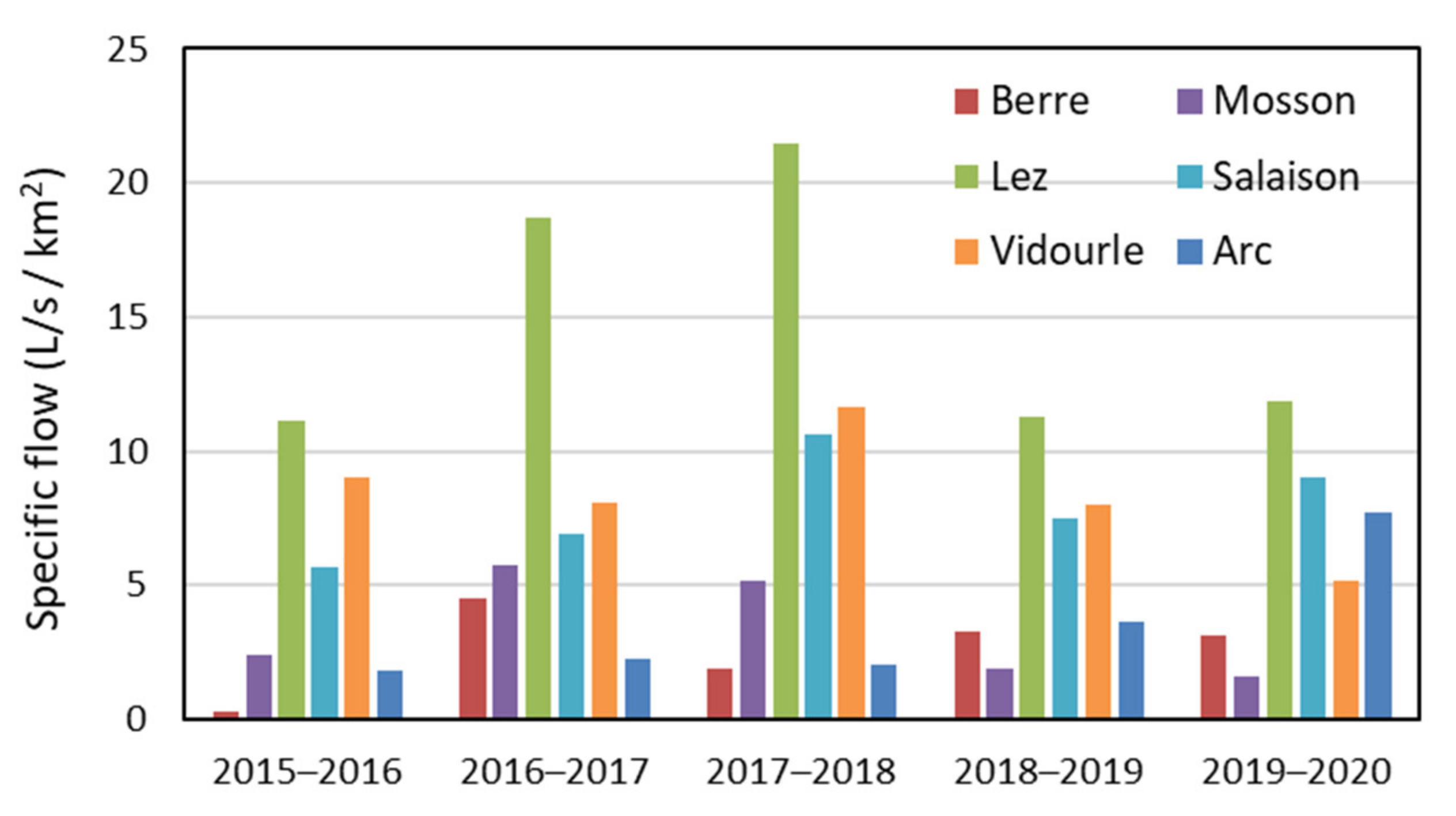
Figure 2 shows the specific flow (L/s/km2) measured on the six rivers. The specific flow is the ratio of the annual mean flow (L/s) to the watershed area (km2). The use of specific flow allows the flows of different rivers to be plotted on the same graph and their magnitudes to be compared.
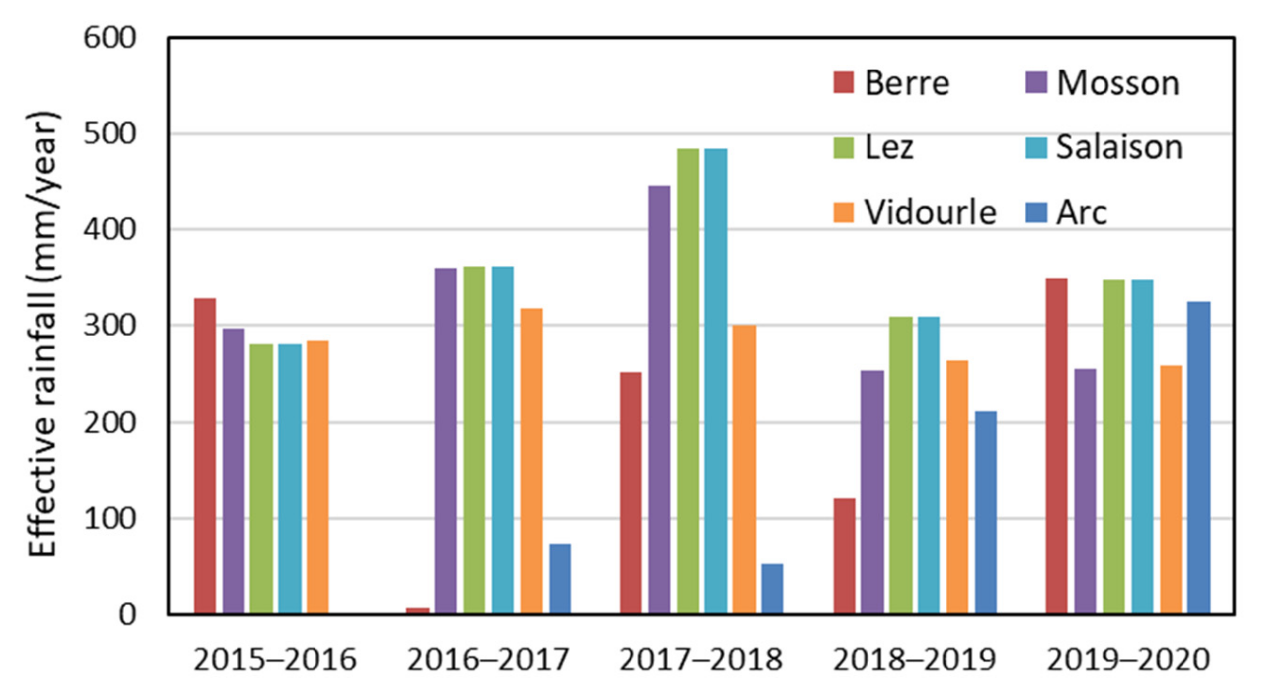
The six rivers have very different specific flows. The Lez has systematically higher values than the other rivers, sometimes more than double. On the other hand, the Berre and the Mosson have very low values compared to the other rivers. These differences cannot be attributed to different amounts of effective precipitation (Figure 3), except in the case of the Arc. Effective precipitation is calculated by taking into account precipitation, potential evapotranspiration and the useful soil reserve (i.e., the temporary water storage in the soil). According to these data, the lowest effective precipitation was observed on the Arc. The Lez and the Salaison (which use the same meteorological station) had the highest effective rainfall.
A previous study [17] showed that the differences between the specific flows calculated from flow measurements or effective rainfalls are explained by the existence of karstic losses and resurgences and by urban sealing. Numerous karstic losses take place on the Berre and Mosson rivers, thus exporting part of the water outside their watersheds. In the case of the Lez, the flow is increased by the existence of an important karstic source upstream of the river and by the exacerbation of runoff due to the sealing of urban surfaces.
2.3. Analytical Procedures
Sampling and transportation of the samples to the laboratory were carried out according to the French regulations and standards in force. The sampling of a river was always carried out at the same point. In low water, when conditions permitted, sampling was performed on foot in the river. In high water, samples were taken in the main flow area from a bridge, on the upstream side. In these cases, water was collected from 50 cm below the surface using a stainless-steel bucket. The bucket and vials for the laboratory were rinsed three times with stream water. The vials were transported to the laboratory overnight without breaking the cold chain. The analyses were performed by a COFRAC-accredited (French Accreditation Committee) laboratory.
TSS were analyzed by gravimetric filtration using a glass fiber filter (NF EN 872 standard). Total phosphorus was analyzed for raw water (water + TSS) by the ammonium molybdate spectrometric method (NF EN ISO 6878). The total nitrogen was obtained by calculation (TKN + nitrate + nitrite). The total Kjeldahl nitrogen (TKN) was analyzed for raw water (water + TSS) by selenium mineralization (NF EN 25663). The nitrate (NO3) and nitrite (NO2) were analyzed for filtered water by the sulfanilamide continuous flow method (NF EN ISO 13395). Ammonium (NH4) and orthophosphate (PO4) were also analyzed for filtered water but were not used in this study.
2.4. Load Calculation Methods
The simplest way to estimate the load is based on the product of the mean flow and the mean concentration:
where Lm is the mean load, Qm is the mean discharge and Cm is the mean concentration.
However, it has been shown that this method gives incorrect results and should therefore never be used [18]. Many other methods have been proposed for estimating loads from flow rates and concentrations. It was not the objective of our study to test these different methods since many previous studies have already done so. Our study focused, in the particular context of Mediterranean rivers, on testing the two most commonly used and recommended methods.
The two methods applied for load estimation over the 5-year period were the flow-weighted mean concentration (FWMC) method (that is, the method recommended in European OSPAR studies) and the flow duration rating curve (FDRC) method (that is, the one recommended by the Swiss FOEN).
The flow duration rating curve method was initially used in [19]. It was proposed to estimate the loads of rivers even when the duration of the discharge record greatly exceeds the period for which sediment data are available. Many authors have subsequently applied, discussed and improved this method, both for suspended and dissolved matter loads (e.g., [20,21,22,23]). This method and its derivatives are regularly used in many studies.
In this method, the average quantity of the load over a given period of time is expressed as
where Lm is the mean load, Qmin and Qmax are the minimum and maximum flows of the river, respectively, C(Q) is the function describing the concentration/flow rating curve and p(Q) is the probability density of Q derived from the flow duration data.
The functions C(Q) and p(Q) are as representative as the flow and concentration datasets are long. The authors in [24] discussed the establishment of the concentration/flow curve and applied this method to various French Mediterranean rivers.
The rating curve approach was first proposed for sediment in [25], where the suspended sediment concentration was expressed as a power function of the discharge:
where C(Q) is the suspended sediment concentration, Q is the flow discharge and a and b are the parameters of the power function.
This method can also be directly applied to the increment scale (e.g., at a weekly time step) of the flow measurement series:
where Q(t) is the flow rate measured at time t. For example, daily average values can be calculated and summed to produce an estimate of the annual discharge.
In [23], the authors note that most concentration data tend to be associated with non-flood flows. The concentration/flow curves under these circumstances tend to be unduly affected by the large number of concentration values at low flows. In [26], a group averaging method is described that determines the average—usually the arithmetic mean or the median—of all values of the dependent variable (mass discharge) for a small range of the independent variable (water discharge). This approach forms the basis of the adapted FDRC method used in our study, where median concentrations are determined over a few flow intervals.
The flow duration rating curve (FDRC) method requires a good definition of the concentration/flow relationship and data covering the entire range of flows and concentrations. It allows the estimation of loads during floods, even if all floods are not sampled. It does not allow flows to be compared year by year if the relationship C(Q) is not stationary in time.
The flow-weighted mean concentration method was initially mentioned in [27]. It has been used for riverine flux calculations of both suspended sediment and other compounds, in numerous studies, with varying sampling frequency and in combination with other calculation methods (e.g., [17,28,29,30,31,32,33]).
In this method, the mean load over a given period of time is expressed as
where Lm is the mean load, Qi is the instantaneous discharge at the time of sampling, Ci is the concentration of an individual water sample and is the mean discharge for the budget period. This method is ideally suited to those situations where there is an abundance of flow information for a tributary but relatively little concentration information [5].
Equation (5) assumes a normal distribution of flow data, which would be unusual for most known rivers. Therefore, the general case would be
where E() and E(Qi) are the expected values of and Qi, respectively [34]. For a normal distribution, the expected value would be the arithmetic mean; for a lognormal distribution it would be the geometric mean. Note, however, that it is not possible to calculate a geometric mean in the case of data series with zero values, which may be the case for flows and nutrients.
In [35], a time-weighted adaptation of Equation (5) was proposed:
where ti is the time interval over which the concentration lasts. It is equal to half the time interval between the previous and next samples. It does not represent the probability over time of the Qi and Ci values measured. This weighting is justified in the case of irregular sampling. However, it can introduce a strong risk of over-representation of the rare events specifically sampled, in an infrequent sampling.
Another adaptation of Equation (5) was proposed in [36] to compensate for the effects of the correlation between discharge and load:
where Li = Qi.Ci, Cov is the covariance and Var is the variance.
This ratio estimator is discussed further in [37,38]. The ratio estimator is termed unbiased since the mean of several ratio estimates tends toward the “true” mean [3]. The bias in the estimate is removed by the term in brackets in Equation (8). As the number (n) of concentration measurements increases, the influence of the bias correction term decreases.
For numerous authors (e.g., those in [4,28,39,40]), the Beale ratio estimator generally provided estimates with minimal bias. For the author in [7], Beale’s method was more appropriate when the correlation between contaminant concentration and streamflow was not strong. In such a case, this method can produce more robust and statistically unbiased results.
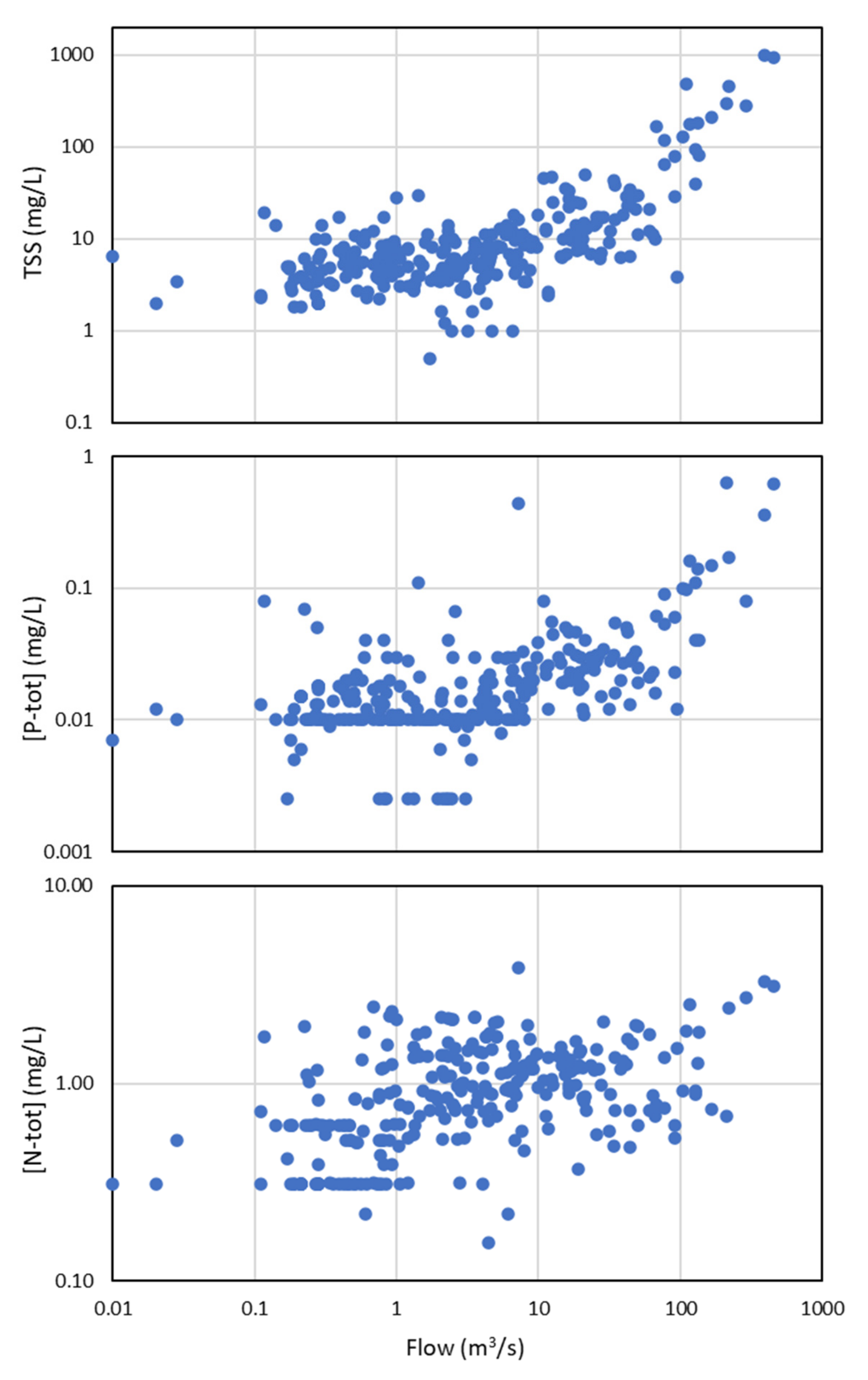
The flow duration rating curve method is mainly based on the relationship established between concentration and flow. However, the concentration/flow graph often shows a strong dispersion of points, making it very difficult to establish a smooth and continuous relationship. Figure 4 shows the concentration/flow relationships observed for the suspended solids, the total phosphorus and the total nitrogen in the Vidourle river. The plot of suspended solids versus flow shows a good correlation between variables. The total phosphorus plot shows the same pattern but with more dispersed values. The total nitrogen shows little correlation, although a positive tendency seems observable.
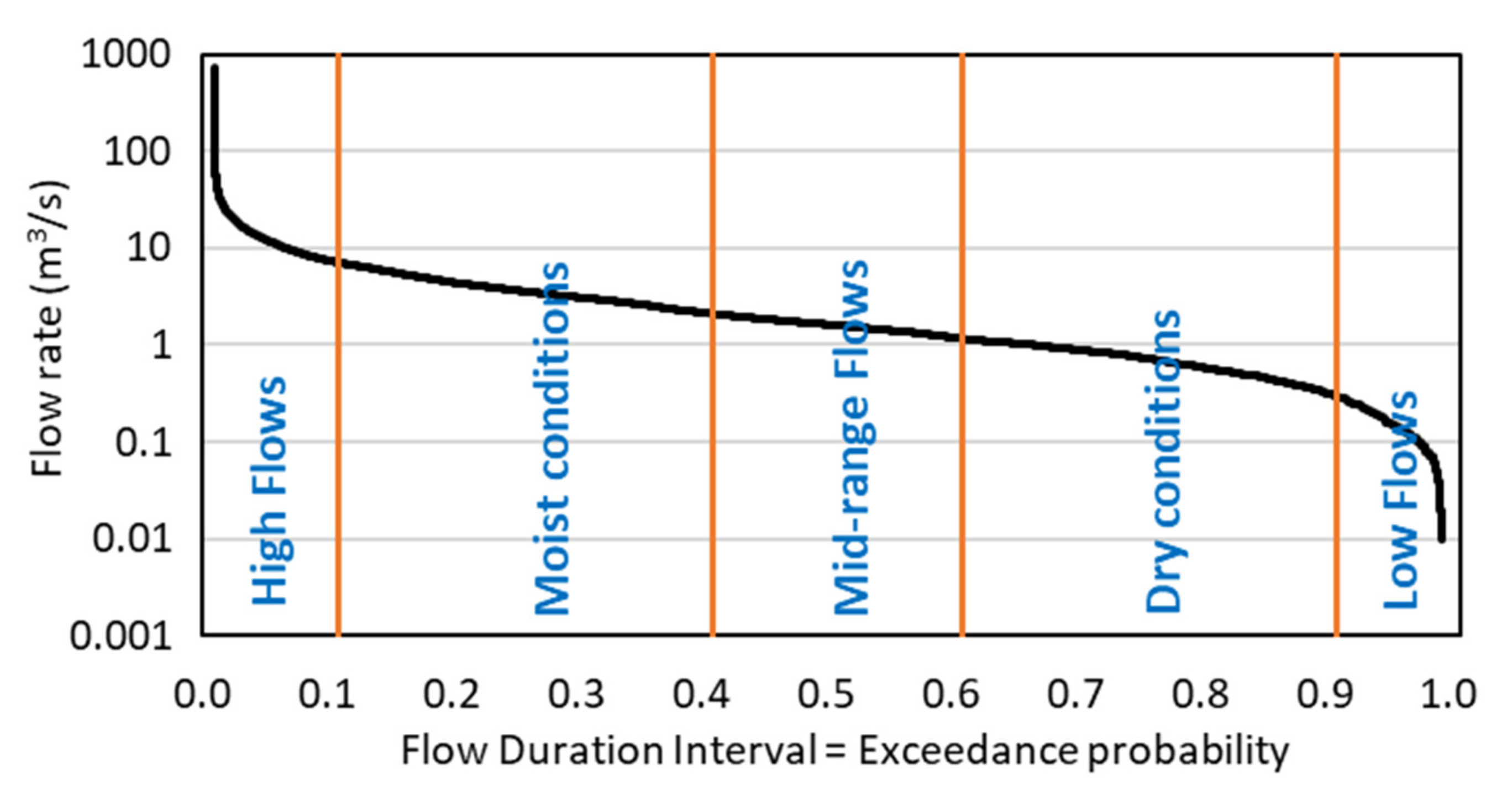
The apparent dispersion of points may be greater when there are fewer data points, which is often the case for higher flows. For these reasons, a flow interval approach is sometimes used. For example, in [41], an interval-based approach to the flow duration curve is proposed. In this EPA method, the duration curve analysis identifies five intervals (Figure 5) that can be used as a general indicator of hydrologic condition (i.e., wet versus dry and to what degree). Flow duration curve intervals can be grouped into several broad categories or zones. For each interval, statistics of concentrations can be calculated, to be used for load estimations or analysis of the water-quality impairment.
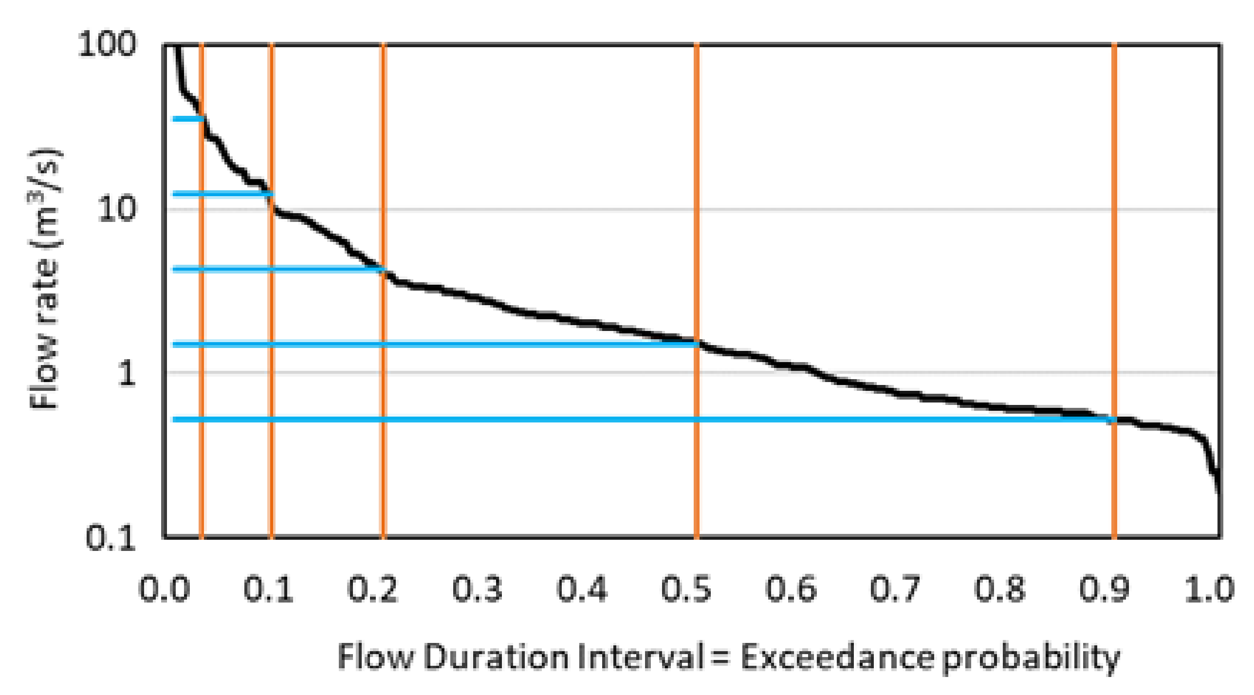
The method implemented in our study used self-adaptative log-equidistant flow intervals specific to each river. These intervals are self-adaptative because only sampled flows are taken into account for their determination. The intervals are determined on the basis of the log-values of the flows and not on their observation probability. Interval lengths are defined so that log(Q sup) − log(Q inf) = constant. Figure 6 illustrates the intervals thus defined. The five intervals on the left have the same “thickness” on the log-scale graph of flows. Due to the presence of zero flow values (leading to an inability to calculate the log values), the low-flow interval is set to the ninetieth percentile of the flow duration curve (i.e., the last decile), as in the EPA method.
3. Results
Nutrients may be dissolved or particulate. The relative importance of these depends on the concentrations of the different forms of nitrogen (nitrate, nitrite, ammonium, organic nitrogen) and phosphorus (mainly dissolved or clay-adsorbed orthophosphate). The average concentrations of all samples (5-year monitoring) were as follows: total nitrogen = 2.083 mg-N/L, nitrate = 1.456 mg-N/L, nitrite = 0.018 mg-N/L, dissolved ammonium = 0.135 mg-N/L, total Kjeldhal nitrogen = 0.609 mg-N/L, total phosphorus = 0.054 mg-P/L and dissolved orthophosphate = 0.054 mg-P/L. Inorganic nitrogen (nitrate, nitrite, dissolved ammonium) represented 77% of the total nitrogen. The total nitrogen was therefore mainly in dissolved form. The particulate forms of nitrogen are clay-adsorbed ammonium and organic nitrogen, the latter being dominant in sediments. Organic nitrogen originates mainly from the decomposition of biological organisms. Dissolved orthophosphate represented 49% of the total phosphorus, indicating that the particulate form represented 51% of the total phosphorus. The average TSS concentration was 66.6 mg/L.
During floods, the average concentrations were as follows: total nitrogen = 2.679 mg-N/L, nitrate = 1.115 mg-N/L, nitrite = 0.019 mg-N/L, dissolved ammonium = 0.267 mg-N/L, total Kjeldhal nitrogen = 1.545 mg-N/L, total phosphorus = 0.286 mg-P/L and dissolved orthophosphate = 0.083 mg-P/L. The particulate form of phosphorus represented 71% of the total, while the particulate form of nitrogen represented 48%. The average TSS concentration was 302.4 mg/L. Floods therefore exacerbate the concentration of TSS, as well as the particulate forms of phosphorus and nitrogen. However, the average concentrations of total nitrogen for the total data series and the flood data (2.083 versus 2.679 mg-N/L) were similar, while those of total phosphorus were very different (0.054 versus 0.286 mg-P/L), as were those for TSS (66.6 versus 302.4 mg/L). The existence of flood data will therefore have a larger impact on TSS and total phosphorus loads, with probably only a small impact on total nitrogen loads.
3.1. Impacts of the Flow Intervals Used in the FDRC Method
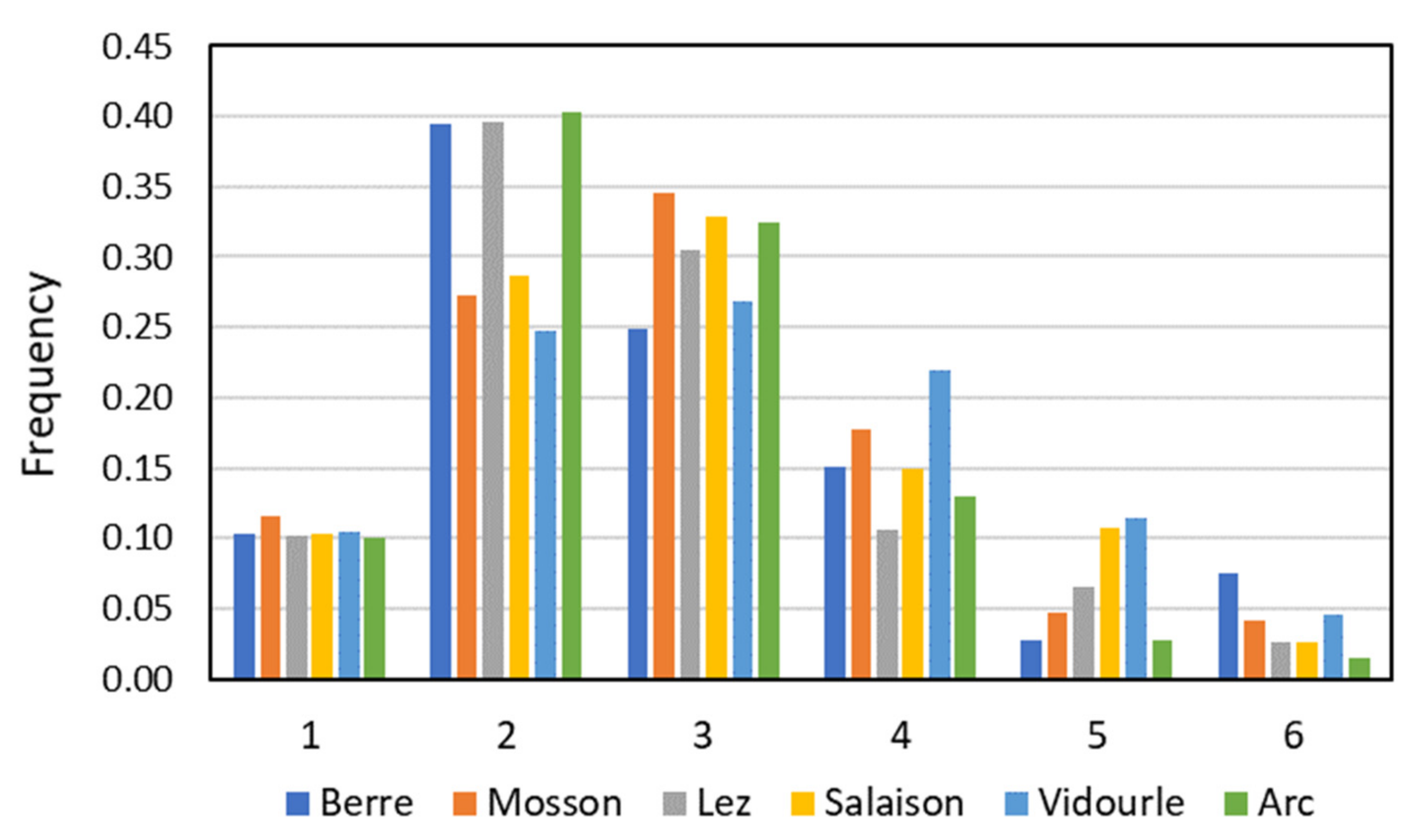
As a reminder, the principle of the FDRC method consists in assigning to each instantaneous flow (e.g., daily or hourly) the concentration corresponding to the flow interval in which the flow was measured. It is thus necessary to define flow intervals and the corresponding concentration values. The main objective of the approach shown in Figure 6 for the definition of flow intervals is to give the highest flows greater representativeness in the calculation of the loads than in the traditional methods. Figure 7 shows the frequency (i.e., the relative number) of samples in each of the six intervals. Although the highest flow classes have less information, no class is without concentration data. The limit values (m3/s) of the six flow intervals are given in Table 4 for each river. The mean values attributed to each interval are indicated in Table 5.
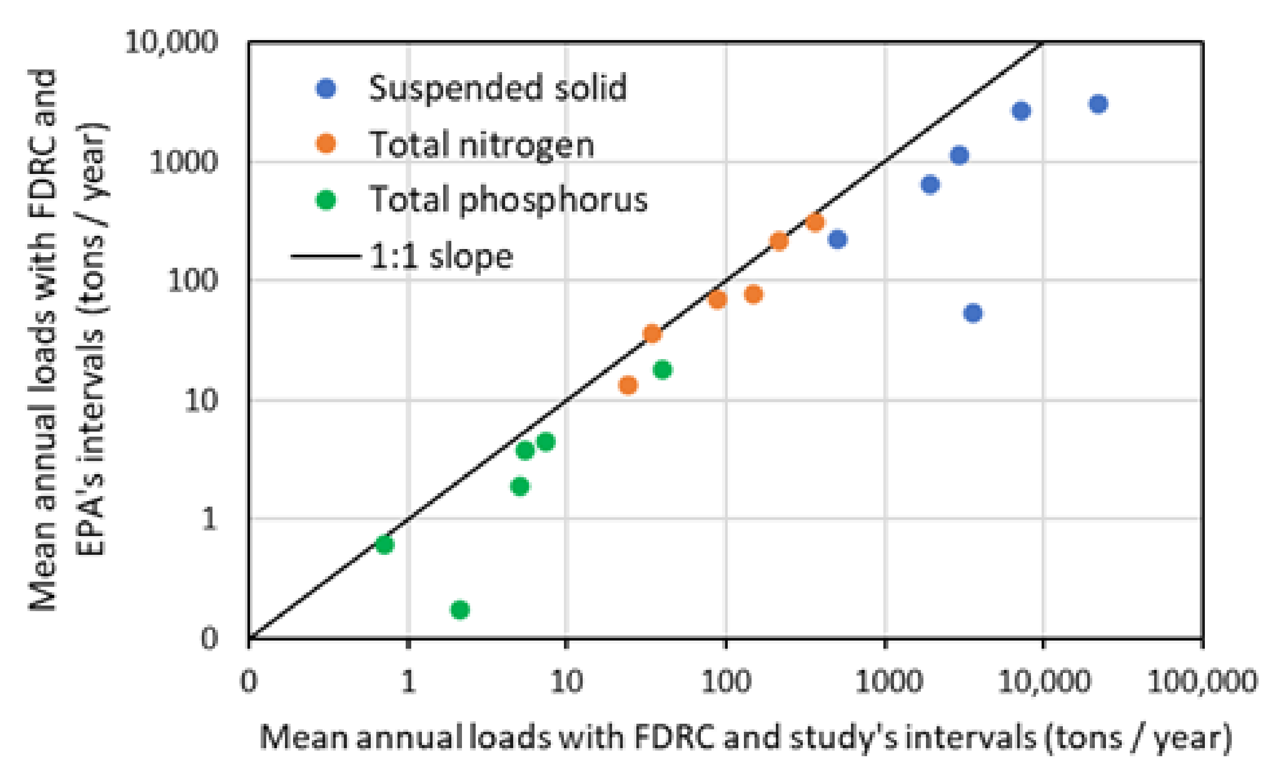
Figure 8 compares the mean annual loads (over the August 2015–July 2020 period) calculated using the FDRC method with the intervals proposed in the EPA approach (Figure 5) and the intervals used in this study (Figure 6). Overall, Figure 8 shows that the total nitrogen loads calculated by the two methods are quite similar (points aligned on the 1:1 slope line), while they differ notably for total phosphorus and even more strongly for TSS. TSS and total phosphorus loads appear to be underestimated when fewer flow intervals are used and there is less focus on high flows.
In Mediterranean rivers, flows are very different during periods without floods (especially low water) and in flood events. During floods, the concentrations of particulate elements are very strongly exacerbated. The FDRC method must therefore take into account these very high concentrations occurring during floods. The definition of the flow intervals must thus give a good representation of the high flows.
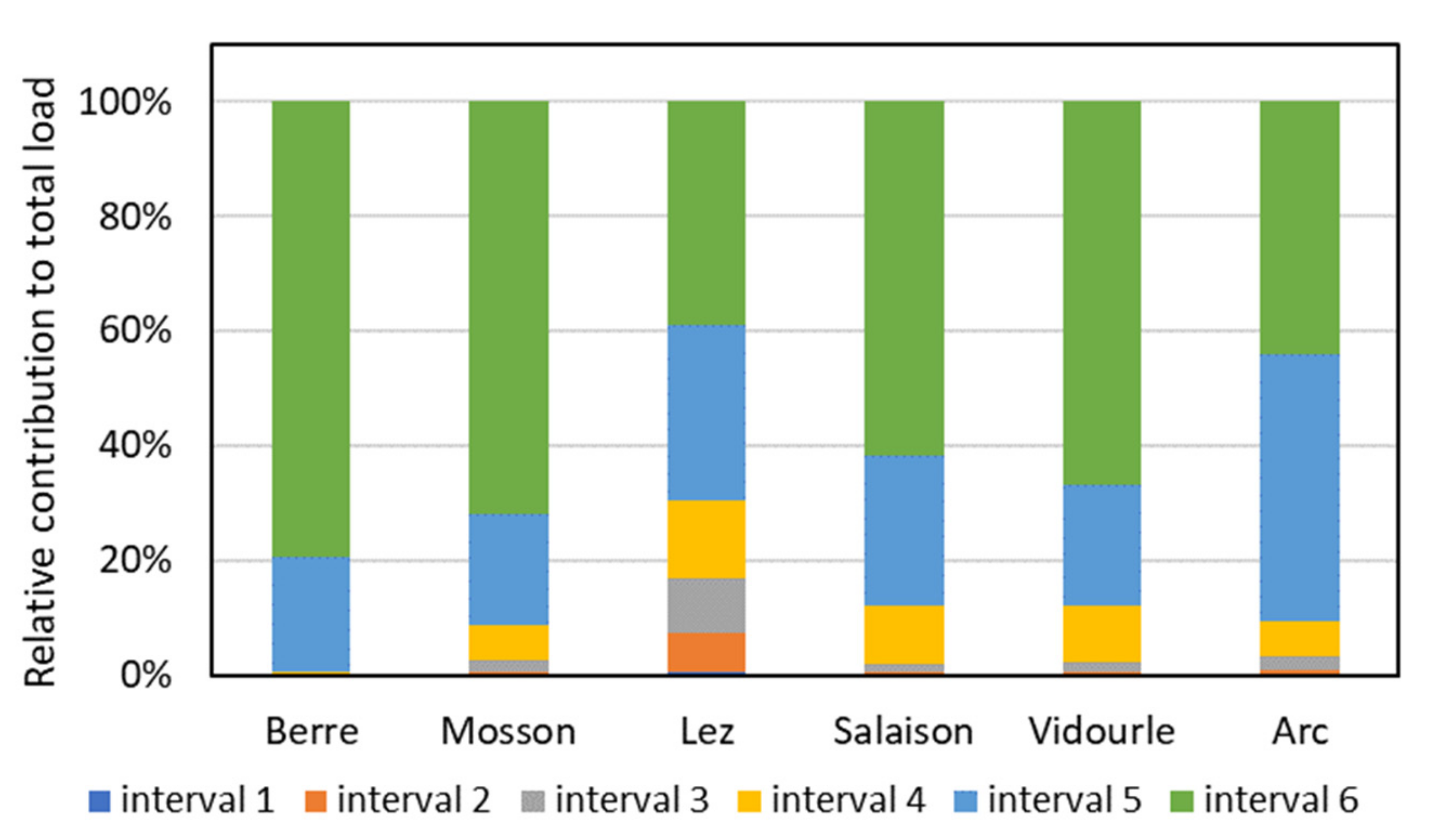
Figure 9 shows the contribution of each flow interval to the mean annual load of TSS. Interval 6 (highest flows) contributes the most to the TSS load, followed by interval 5. The low-flow intervals contribute very little to the exported load. For the Berre, 80% of the load is contributed by interval 6. For the other rivers, intervals 6 and 5 contribute between 70 and over 90% of the total load.
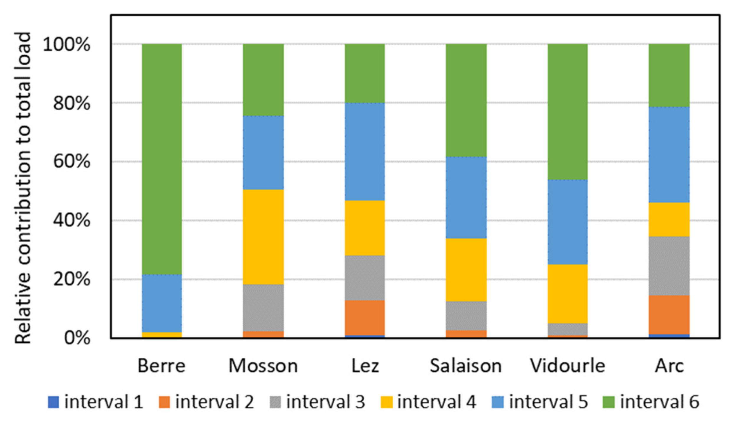
For the load of total phosphorus (Figure 10), the pattern is similar for the Berre. For the other rivers, interval 6 is less preponderant, and intervals 4 and 3 are more so.
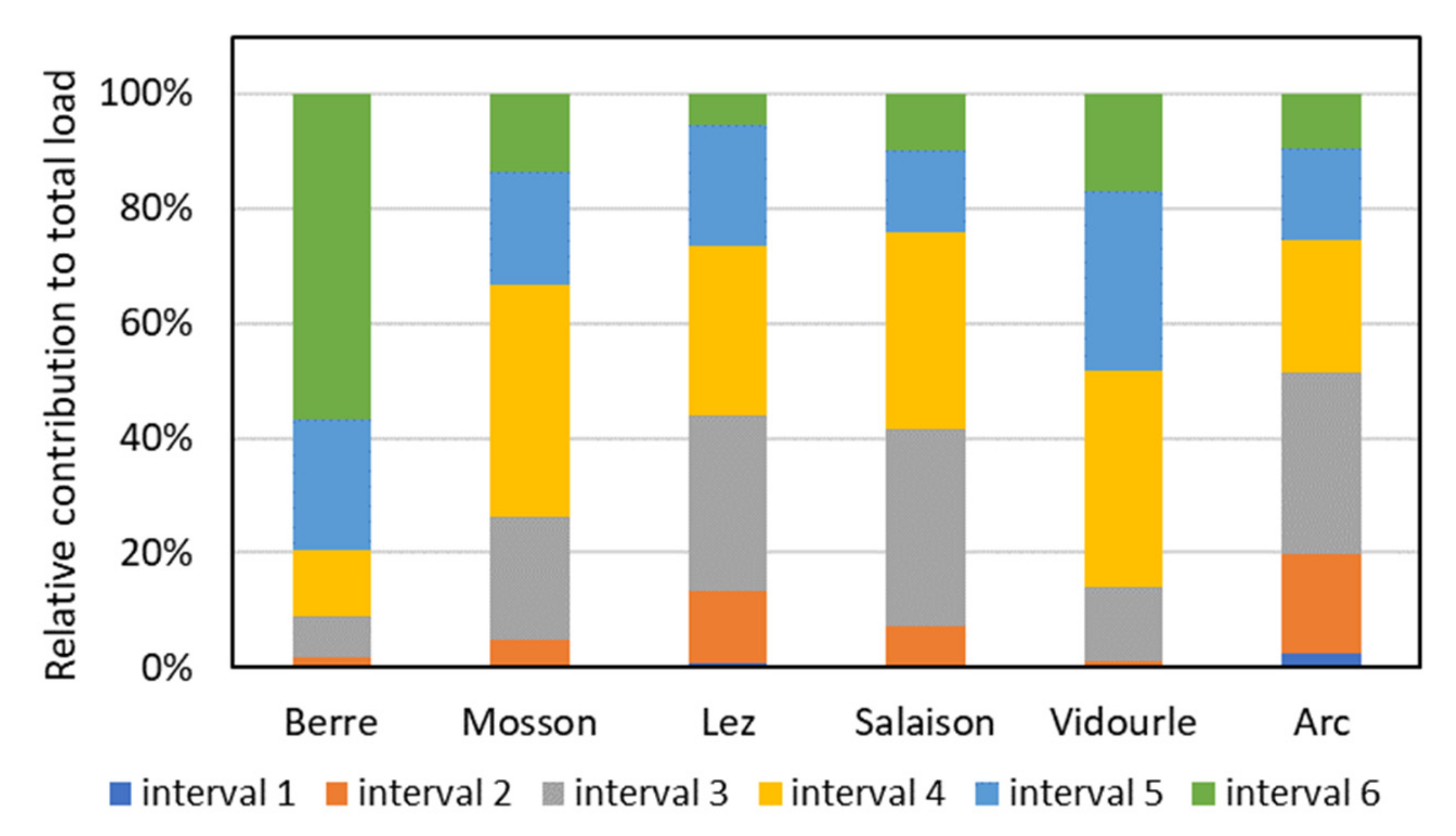
For the load of total nitrogen (Figure 11), the shift in contributions towards the low-flow intervals is increased. Interval 4 shows a large contribution for most rivers, and the contribution of interval 3 is also significant.
The preponderance of high flow intervals appears to correlate with the importance of particulate forms in the exported loads, whereas the importance of intermediate flow intervals appears to be related to dissolved forms.
3.2. Comparison of Annual Loads Calculated by the FWMC and FDRC Methods
Table 6 gives the mean annual loads of suspended solids, total nitrogen and total phosphorus calculated by the FWMC and FDRC methods for the six rivers.
The loads calculated using the FWMC method are very different from those obtained with the FDRC method. The ratios calculated for the loads of TSS obtained from the two methods are very high (average = 4.9). They vary between 4.7 and 6.0, except for the Arc river, which has a lower ratio of 2.4. The ratios of the loads calculated for the total phosphorus are high, varying between 2.5 and 6.2 (average = 3.5), except for the Arc river again (ratio of 1.6). Except for the Berre river (with a ratio of 3.2), the ratios of the loads calculated for total nitrogen using the two methods are close to 1. This means that the load of total nitrogen is influenced only a little by the method used.
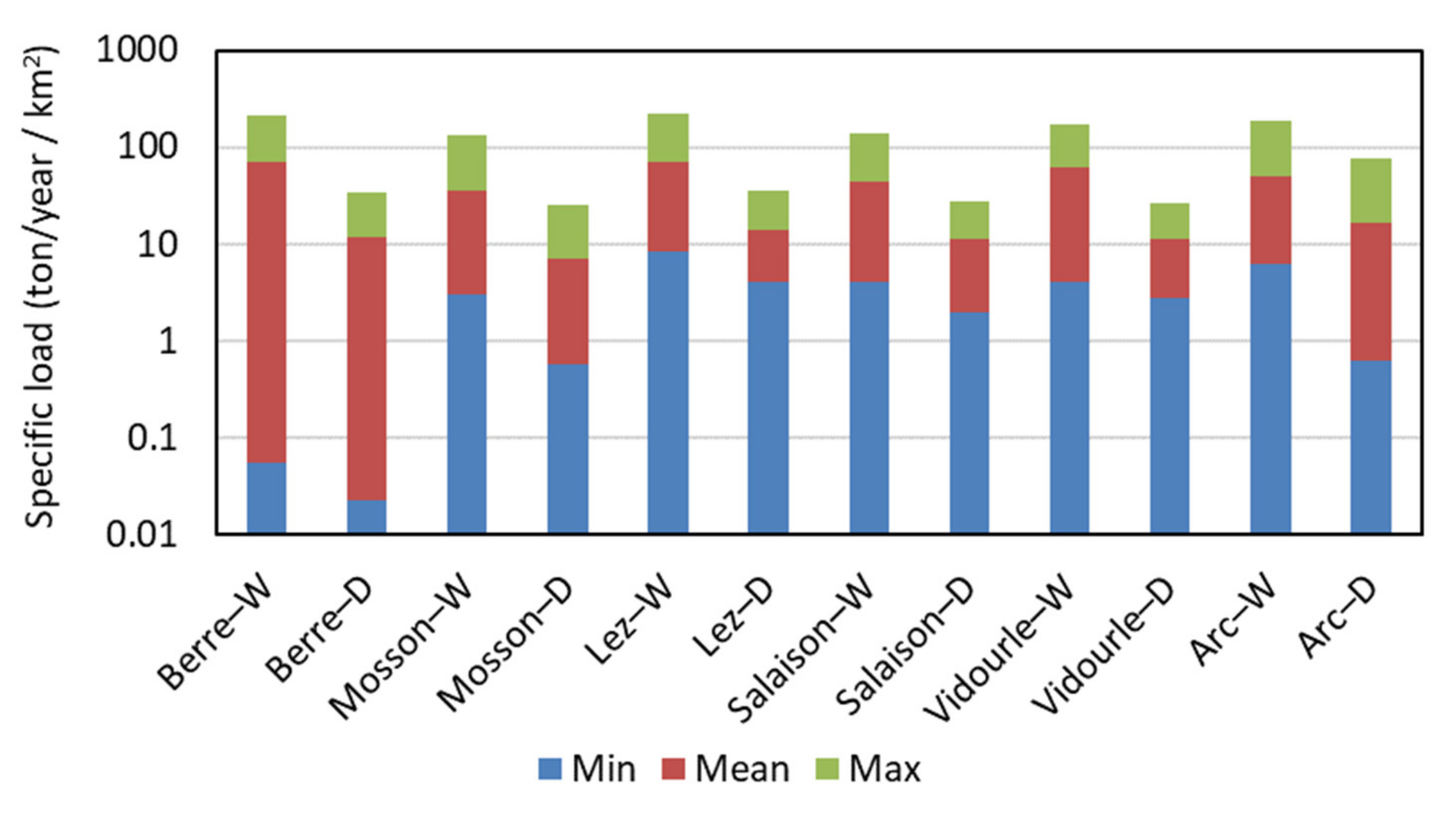
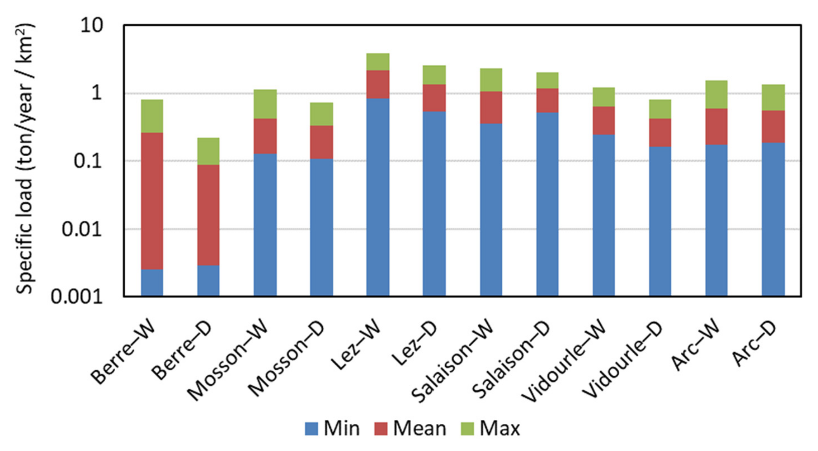
The mean loads cannot be directly compared between rivers due to their very different areas. For this reason, the following figures use the specific loads, i.e., the loads divided by the watershed area. Figure 12 shows the minimum, average and maximum values of the five annual specific loads of suspended solids calculated by the two methods. Detailed plots of annual loads for the five years are provided in the Supplementary Materials.
The mean specific loads are very variable from one river to another. Mean loads calculated by the FWMC method are sometimes very high, exceeding 100 tons/km2 in 8 cases out of 30. They are also sometimes very low, at less than 20 tons/km2 in 13 cases out of 30. Mean loads calculated by the FDRC method are significantly lower than those calculated by the FWMC method and rarely exceed 20 tons/km2.
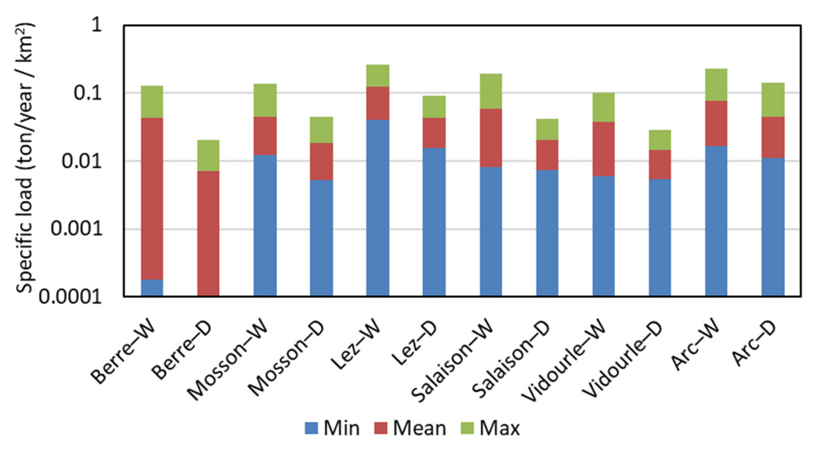
Figure 13 shows the specific loads of total phosphorus (ton/year/km2) calculated using both methods. The results for the total phosphorus are presented before those for the total nitrogen, due to their similarity to the sediment loads. Actually, particulate phosphorus accounts for a high fraction of phosphorus loads in rivers, due to the strong affinity between orthophosphate (the major dissolved form of phosphorus) and particulates. Specific loads of total phosphorus calculated using the FWMC method exceed 0.1 ton/km2 in 4 cases out of 30 and are between 0.05 and 0.1 ton/km2 in 7 cases. As previously seen for the suspended solids, the loads calculated using the FDRC method are very different and are lower than those obtained from the FWMC method.
Figure 14 shows the specific loads (ton/year/km2) of total nitrogen calculated by the two methods. The loads are fairly similar for the two methods, and the global pattern is very different from the patterns of TSS and total phosphorus previously discussed.
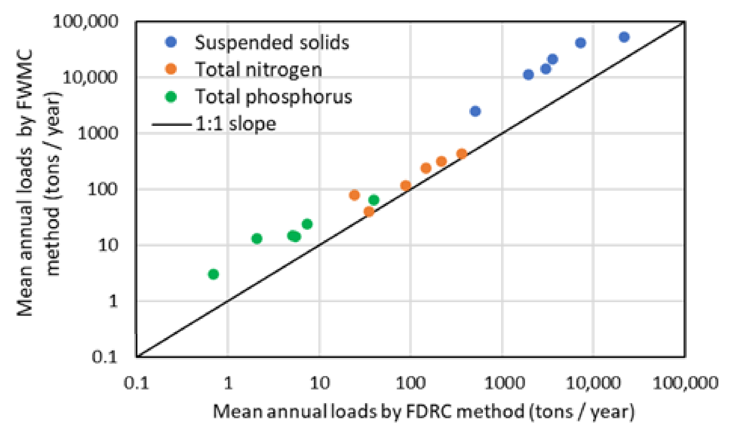
Figure 15 clearly shows the significant differences between the loads calculated by the two methods, especially for TSS and total phosphorus. For total nitrogen loads, the results calculated by both methods are close to the 1:1 slope line. Although the results do not allow us to clearly state that the FWMC method overestimates the values for suspended solids and total phosphorus, Figure 15 seems support this hypothesis.
3.3. Test of the Beale’s Correction Factor in FWMC Method
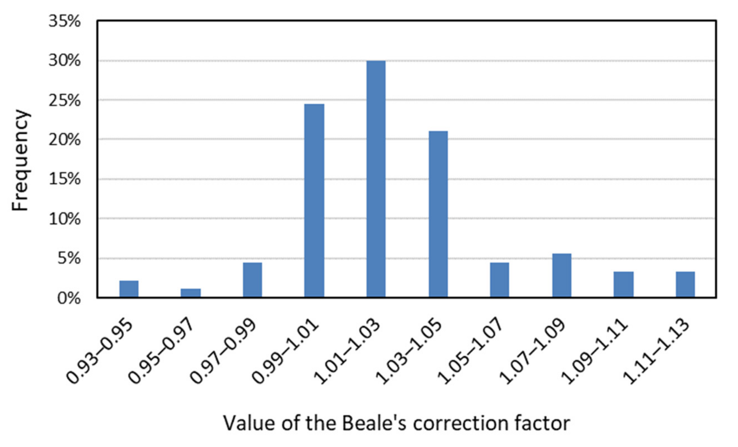
In [37], a correction factor was developed that adjusts for the bias induced by the correlation between discharge and load, as described in Equation (8). Load estimation is termed unbiased since the mean of several ratio estimates tends toward the “true” mean [5]. As the number of concentration measurements increases, the influence of the bias correction term decreases. The Beale correction factor was calculated for all annual load estimates (5 years × 3 parameters × 6 rivers) in order to evaluate the improvement that may result from this factor. Figure 16 shows the distribution of the values calculated. They range between 0.93 and 1.13, with most of them between 0.99 and 1.05 (75.6% of the values), which indicates that this factor would modify the value of the loads calculated by the FWMC method by only a little. Taking this correction factor into account does not allow the results calculated by the two methods to be closer.
3.4. Importance of the Flood Samplings into the FWMC Method
Table 3 shows that the proportion of samples taken during flood events was considerably higher than 5%, i.e., than the percentage considered to define a flood event (5% exceedance of the flow duration curve). The data collected from flood periods are over-represented with regard to the statistics of occurrence of these events. This over-representation is the result of the intentionally large sampling of floods in this study.
Table 7 provides the mean annual loads calculated by the FWMC method without flood data, the ratio between these loads and those calculated using the FWMC method using all data (flood and non-flood data) and the ratio between these loads and those calculated using the FDRC method.
The ratios of loads calculated by FWMC with or without flood data range between 4 and 32 for the TSS and between 2 and 24 for the total phosphorus but only between 1 and 4 for the total nitrogen. The Berre river shows the highest ratio and the Arc shows the lowest. Ratios of loads calculated using FDRC and FWMC without flood data vary between 1.5 and 9.5 for TSS, between 1.1 and 3.8 for total phosphorus and between 0.9 and 1.1 for total nitrogen.
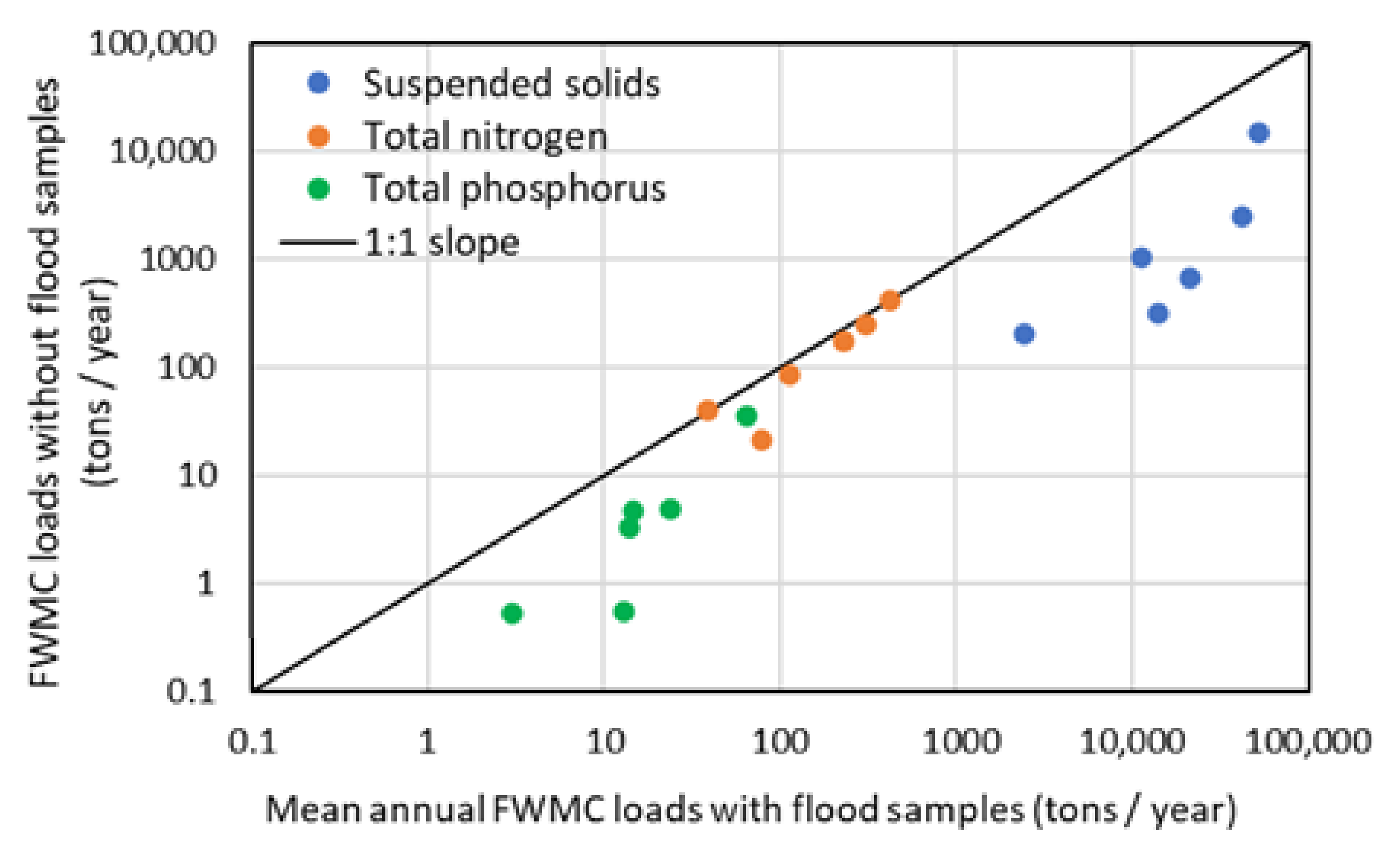
Figure 17 compares the loads calculated by the FWMC method with all data or excluding flood samples. Loads of TSS and total phosphorus calculated with the FWMC method without flood data are much lower than those calculated with the FWMC method using flood data (all the points are far below the 1:1 slope line). The loads calculated for the total nitrogen using the two methods are close to the 1:1 slope, except for one orange point, indicating that the load values are similar.
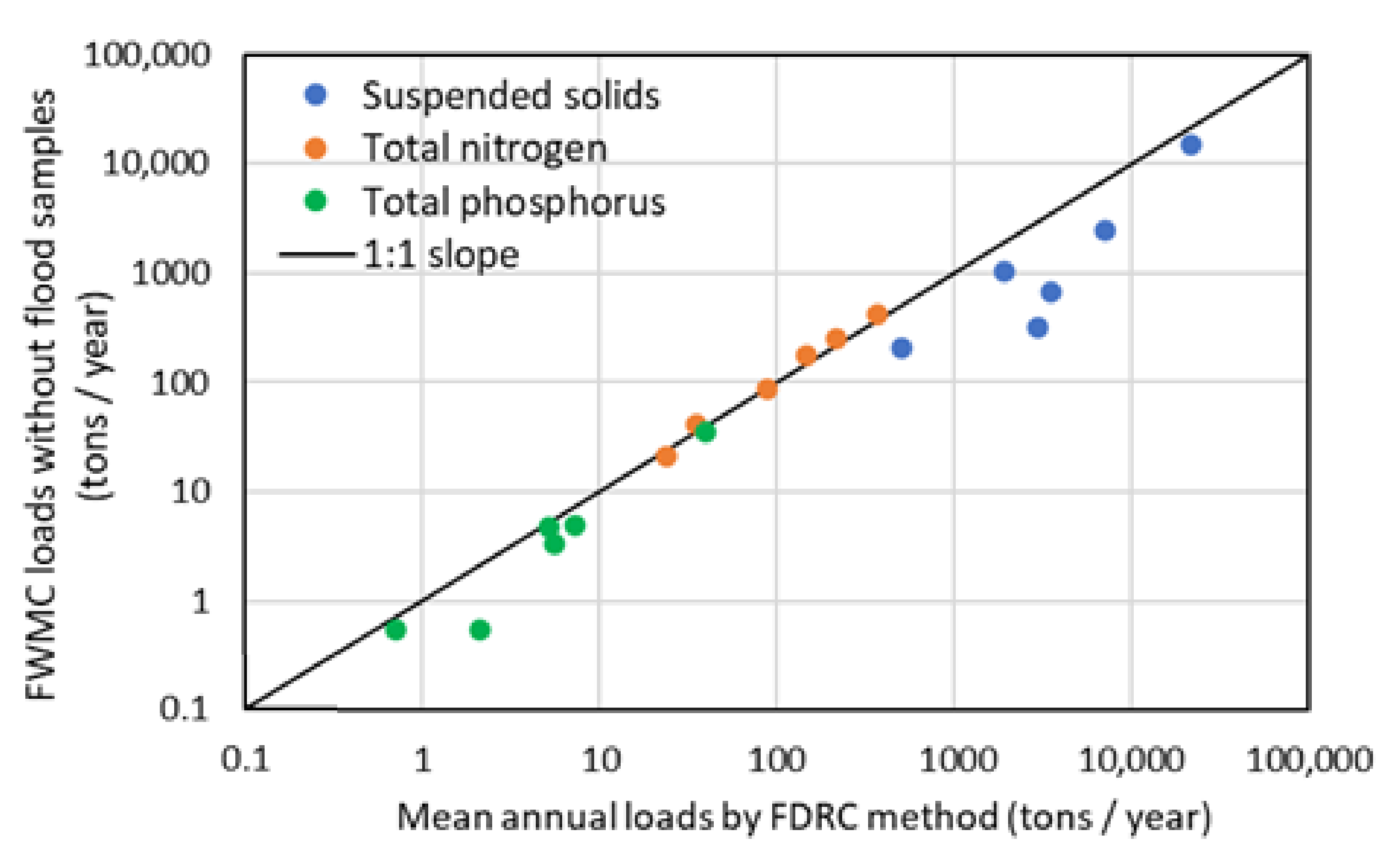
Figure 18 shows the difference between the loads calculated using the FDRC method and the FWMC method without the flood samples. The differences are very small for total nitrogen, significant for total phosphorus and more important for TSS.
For TSS and total phosphorus, the loads calculated using the FDRC method are systemically intermediate between those calculated using the FWMC method with and without the flood data. For total nitrogen, the differences between loads calculated using the three methods are small. All these results show that the inclusion or exclusion of flood data in the FWMC method has a significant influence on the magnitude of the calculated loads. The FWMC method appears to be strongly influenced by the flood sampling density when calculating the loads for the particulate forms (suspended solids and adsorbed phosphorus). It is very sensitive to the presence and the number of high-concentration measurements related to flood events. For the Mediterranean rivers and for the particulate forms, the FWMC method does not therefore seem to be directly applicable. Too many samples induce an overestimation of the flows, while too few samples induce an underestimation.
3.5. Impact of the Number of Flood Samples Used in the FWMC Method
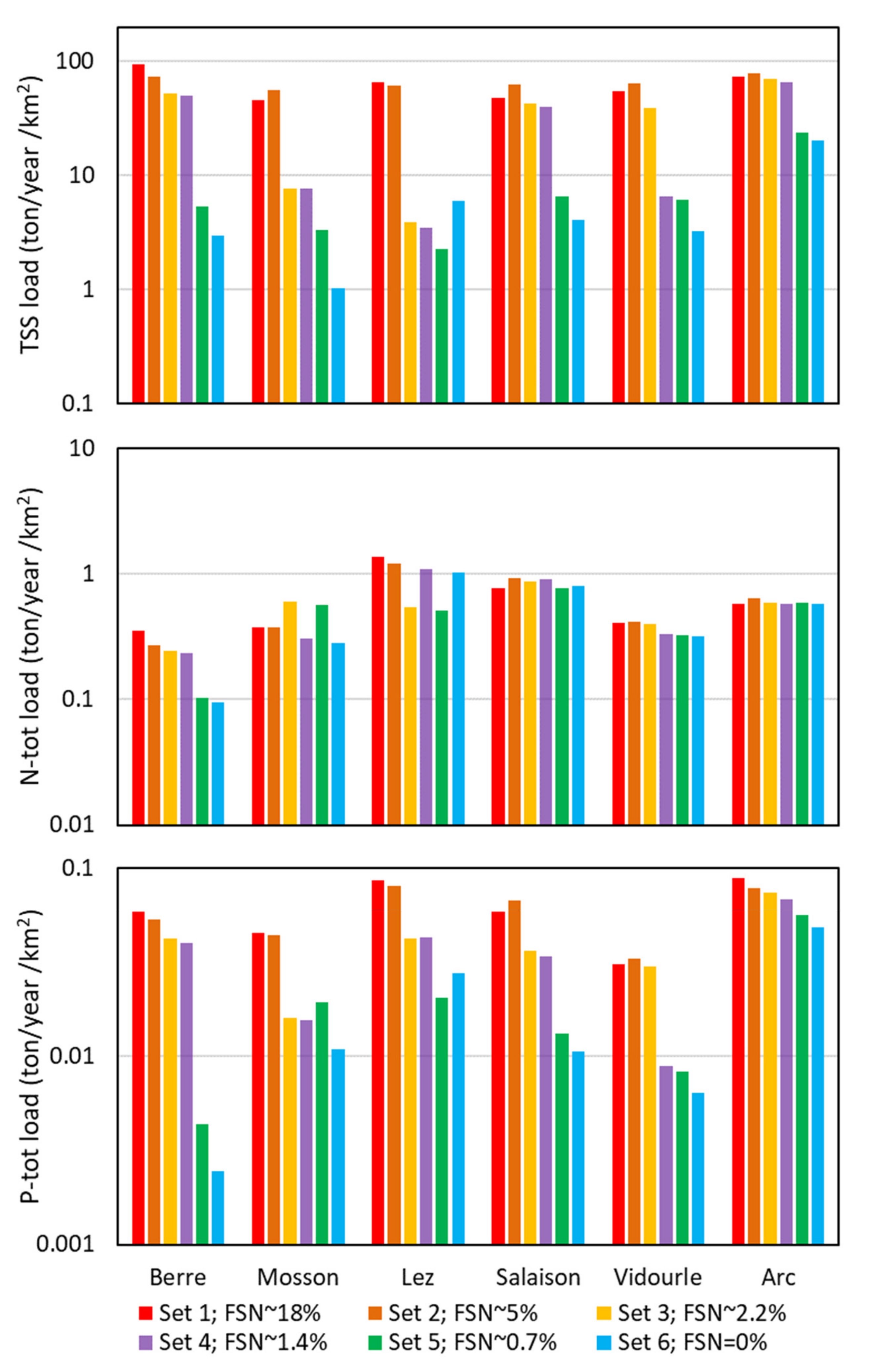
In order to test the influence of the number of samples taken during flood periods on the calculation of loads by the FWMC method, some of the samples were randomly removed from the initial dataset. Different datasets were thus obtained:
- Set 1: total series, where samples taken during flood periods represent about 18.5% of the samples (Table 3);
- Set 2: number of samples during flood periods respecting the 5% exceedance frequency used to define flood events (flow rate > threshold);
- Set 3: number of flood samples half that respecting the threshold statistics (< 2.5% of total samples);
- Set 4: only two samples during the 5-year monitoring period (~1.4% of total samples);
- Set 5: only one sample during the 5-year monitoring period (~0.7% of total samples);
- Set 6: data series excluding flows above the threshold (0% of total samples).
Figure 19 shows the loads calculated with these different datasets. As previously mentioned, total nitrogen loads varied relatively little from one dataset to another, only varying by a factor of 2 to 3 at most. Conversely, suspended solids and total phosphorus loads varied significantly, sometimes by a factor of more than 15. Overall, the use of flood data respecting the 5% frequency of exceedance used for the establishment of the thresholds did not modify the calculated loads very much. In some cases, the loads were even higher than those obtained from the total dataset, since the randomly removed samples may correspond to high or low concentrations. A noticeable decrease in the load was only observed for percentages of flood samples much smaller than 5%.
4. Conclusions
Protecting the quality of coastal water bodies (lagoons, mangroves, seas and oceans) requires the assessment of contaminant discharge brought by coastal rivers. This involves measuring stream flow rates and associated concentrations. While water flows are often known almost continuously (high-frequency measurements), concentrations are only known with a much lower frequency (weekly or monthly in most water-quality monitoring studies).
Among existing methods for estimating total suspended solids (TSS) and nutrient loads, the most widely used and recommended methods are the flow-weighted mean concentration method (FWMC) and the flow duration rating curve method (FDRC). Depending on the rivers and the sampling frequencies, these two methods give closer or more distant results. The FWMC method only uses the concentration data for the period covered by the flux calculation, while the FDRC method uses all the historical data to determine a concentration/flow relationship. The FWMC method is therefore constrained by the data available over each studied period, while the FDRC method is conditioned by the representativeness and uniqueness of the concentration/flow relationship. Adding new flood data as the quality monitoring progresses improves the relationship. The more flood data used, the better the concentration/flow relationship and the better the load estimate using the FDRC method.
In the Mediterranean basin, the hydrology is characterized by infrequent but very intense rainfall events. The flows taking place during these periods last only a few hours to a few days but can represent the largest part of the annual flow. The loads associated with these events can also account for most of the annual load. The flows generated by these Mediterranean storm events can represent a significant part of the annual volume. These events also exacerbate erosion and the transport of suspended or dissolved matter. Concentrations sometimes increase in proportion to the flow, particularly for suspended solids and total phosphorus.
The monitoring performed over five years on six rivers showed that average concentrations of TSS and total phosphorus during flood events were significantly higher than those observed during non-flood periods. This difference was not observed for total nitrogen. This could be attributed to the fact that total phosphorus is primarily present in particulate form (adsorbed on clays) during floods and is thus associated with TSS.
This study showed the importance of flood data in the calculation of suspended solids and nutrient loads. The calculated loads illustrated the inadequacy of the FWMC method for calculating TSS and total phosphorus loads. A lack of flood data leads to underestimation of these loads, while the inclusion of only some flood data can lead to significant overestimation of the loads. These problems have little or no effect on total nitrogen loads.
A correspondence between the relative number of flood samples and the relative probability of flows is not sufficient to ensure the calculation of reliable loads for TSS and total phosphorus using the FWMC method. This can be attributed to the strong dependence of the concentrations on the magnitude of the flow. This problem is exacerbated in the Mediterranean context, where rainfall events are very violent and induce very strong erosion. The FWMC method would seem to be able to provide correct results, provided the representativeness of the flood samples taken into account by the method respect the probability of instantaneous loads (and not that of floods). Unfortunately, this cannot be achieved in real time as for flows. It may require an a posteriori correction, in the light of the instantaneous loads measured. This possible area of improvement requires further investigation.
For Mediterranean rivers, the calculation of TSS and total phosphorus loads should be performed preferentially or exclusively using the FDRC method. However, this study showed the impact of under-representing flood flows when defining the flow intervals used by the FDRC method. A too-large interval for high flows leads to underestimation of the average flood concentration and thus the calculated load. This affects TSS and total phosphorus loads, though it has little effect on total nitrogen.
The concentration of total nitrogen is not very dependent on the flow. FDRC and FWMC methods can therefore be used, giving statistically close results without particular precautions regarding the number of floods taken into account in the FWMC method or the definition of flow intervals in the FDRC method.
This study allows us to make recommendations on monitoring and calculations. While total nitrogen concentrations appear to be fairly independent of flow, total phosphorus concentrations are more strongly correlated with flow due to the preponderance of the particulate form of phosphorus, especially during floods. It is therefore necessary for water-quality monitoring to include sampling during flood periods, despite the difficulties of realization of these samplings under the weather and hydrologic conditions.
The estimation of loads, especially in particulate forms, should favor the consideration of high flow rates. This leads us to recommend the use of the FDRC method and the definition of flow intervals favoring higher flow classes. The estimation of loads, in particular the particulate forms, should give priority to the consideration of high flow rates. This leads to the recommendation to use the FDRC method and to define flux intervals particularly representing high flux classes.
In the case of ungauged watersheds or those without water-quality monitoring, approaches of varying complexity can be used to estimate the orders of magnitude of the sediment and nutrient loads. These approaches can range from empirical methods based on the use of factors controlling the production and fate of TSS and nutrients to models simulating the processes involved.
The European Soil Data Centre (ESDAC; esdac.jrc.ec.europa.eu), a Joint Research Centre established by the European Commission [42], has applied a modified version of the Revised Universal Soil Loss Equation (RUSLE) model (RUSLE2015) to estimate soil loss in Europe [43]. This approach uses different input factors: rainfall erosivity, soil erodibility, cover management, topography and support practices. The data for soil loss rates calculated with this model are available at 100 m resolution from the ESDAC website. The average losses estimated by RUSLE2015 for the six studied watersheds were calculated via GIS.
The soil loss rates ranged between 189 and 452 tons/year/km2, while the TSS loads calculated with the FDRC method varied between 9.9 and 30.1 tons/year/km2 (TSS loads from FWMC method ranged between 45.9 and 94.8 tons/year/km2). The soil losses estimated by RUSLE2015 were about 30 times higher than the estimated TSS loads downstream of the watersheds. The two types of values cannot be directly compared, however, since it is possible that some of the eroded soils form sediment downstream of their erosion zone and do not generate TSS loads at the watershed outlet. Therefore, the soil losses estimated by RUSLE2015 should be considered to represent the maximum soil erosion potential.
A promising approach has recently been proposed for estimating TSS- and particle-facilitated contaminant transport in watersheds. In [44], high-frequency in situ turbidity measurements were used as a proxy for total phosphorus, while in [45], high-frequency in situ turbidity measurements were used as a proxy for adsorbed polycyclic aromatic hydrocarbons (PAHs). In both cases, the authors found a good correlation between turbidity measurements and TTS concentrations. If a relationship can be established between adsorbed contaminant concentrations and TSS, as in their studies, high-frequency turbidity monitoring could become a relevant proxy that can be directly coupled to flow measurements for real-time estimation of exported loads.
Supplementary Materials
The following are available online at https://0-www-mdpi-com.brum.beds.ac.uk/article/10.3390/hydrology9060110/s1, Figure S1. Comparison of the flows sampled during the quality monitoring (in red) with the flows observed during the last ten years (in blue); Figure S2. Specific load (ton/year/km2) of total sus-pended solids calculated on the six watersheds by the Flow Weighted Mean Concentration (FWMC) method; Figure S3. Specific load (ton/year/km2) of total suspended solids calculated on the six watersheds by the Flow Duration Rating Curves (FDRC) method; Figure S4. Specific load (ton/year/km2) of total phosphorus calculated on the six watersheds by the Flow Weighted Mean Concentration (FWMC) method; Figure S5. Specific load (ton/year/km2) of total phos-phorus calculated on the six watersheds by the Flow Duration Rating Curves (FDRC) method; Figure S6. Correlation between specific load (ton/year/km2) of total suspended solids and total phosphorus calculated by the Flow-Weighted Mean Concentration (FWMC) method; Figure S7. Correlation between specific load (ton/year/km2) of total suspended solids and total phosphorus calculated by the Flow Duration Rating Curves (FDRC) method; Figure S8. Specific load (ton/year/km2) of total nitrogen calculated on the six watersheds by the Flow-Weighted Mean Concentration (FWMC) method; Figure S9. Specific load (ton/year/km2) of total nitrogen calcu-lated on the six watersheds by the Flow Duration Rating Curves (FDRC) method; Figure S10. Correlation between specific load (ton/year/km2) of total nitrogen calculated by FWMC and FDRC methods; Figure S11. Specific mean loads calculated with the FDRC method and with the FWMC method considering or not the flood samples (TSS = total suspended solids; Figure S12. Ratio of loads calculated by the FWMC method considering or not the flood samples; Figure S13. Ratio of loads calculated by the FWMC method considering the flood samples and the FDRC method; Figure S14. Ratio of loads calculated by the FDRC method and the FWMC method without the flood samples.
Author Contributions
Conceptualization, O.B., S.S.-P. and H.G.; formal analysis, O.B.; investigation, S.S.-P.; methodology, O.B., S.S.-P., H.G. and A.G.; project administration, A.G.; software, H.G.; supervision, A.G.; writing—original draft, O.B. and S.S.-P.; writing—review and editing, H.G. and A.G. All authors have read and agreed to the published version of the manuscript.
Funding
This study was carried out thanks to funding by the Rhône Méditerranée Corse Water Agency.
Institutional Review Board Statement
Not applicable.
Informed Consent Statement
Not applicable.
Data Availability Statement
The data used in this paper are available free of charge on the Internet for hydrometric flow (hydro.eaufrance.fr) and water-quality data (naiades.eaufrance.fr) (accessed on 11 April 2022).
Conflicts of Interest
The authors declare no conflict of interest.
References
- Nava, V.; Patelli, P.; Rotiroti, M.; Leoni, B. An R package for estimating river compound load using different methods. Environ. Model. Softw. 2019, 117, 100–108. [Google Scholar] [CrossRef] [Green Version]
- Abolfathi, S.; Pearson, J. Application of smoothed particle hydrodynamics (SPH) in nearshore mixing: A comparison to laboratory data. Coast. Eng. Proc. 2016, 1, 16. [Google Scholar] [CrossRef]
- Borzooei, S.; Amerlinck, Y.; Abolfathi, S.; Panepinto, D.; Nopens, I.; Lorenzi, E.; Meucci, L.; Zanetti, M.C. Data scarcity in modelling and simulation of a large-scale WWTP: Stop sign or a challenge. J. Water Process Eng. 2019, 28, 10–20. [Google Scholar] [CrossRef] [Green Version]
- Preston, S.D.; Bierman, V.J.; Silliman, S.E. An evaluation of methods for the estimation of tributary mass loads. Water Resour. Res. 1989, 25, 1379–1389. [Google Scholar] [CrossRef]
- Dolan, D.M.; Yui, A.K.; Geist, R.D. Evaluation of river load estimation methods for total phosphorus. J. Great Lakes Res. 1981, 7, 207–214. [Google Scholar] [CrossRef]
- Walling, D.E. Assessing the accuracy of suspended sediment rating curves for a small basin. Water Resour. Res. 1977, 13, 531–538. [Google Scholar] [CrossRef]
- Ferguson, R.I. Accuracy and precision of methods for estimating river loads. Earth Surf. Processes Landf. 1987, 12, 95–104. [Google Scholar] [CrossRef]
- Cohn, T.A. Recent advances in statistical methods for the estimation of sediment and nutrient transport in the rivers. Rev. Geophys. 1995, 33 (Suppl. S2), 1117–1123. [Google Scholar] [CrossRef]
- Aulenbach, B.T.; Burns, D.A.; Shanley, J.B.; Yanai, R.D.; Bae, K.; Wild, A.D.; Yang, Y.; Yi, D. Approaches to stream solute load estimation for solutes with varying dynamics from five diverse small watersheds. Ecosphere 2016, 7, e01298. [Google Scholar] [CrossRef] [Green Version]
- OSPAR Commission. OSPAR Guidelines for Harmonised Quantification and Reporting Procedures for Nutrients (HARP-NUT). 2004. Available online: https://www.ospar.org/documents?d=32400 (accessed on 14 April 2022).
- Grasso, D.A.; Jakob, A. Charge de sédiments en suspension. Gas Wasser Abwasser 2003, 12, 898–905. [Google Scholar]
- PERSEUS—UNEP/MAP Report. Atlas of Riverine Inputs to the Mediterranean Sea; 2015; ISBN 978-960-9798-17-4. Available online: www.perseus-net.eu/assets/media/PDF/5567.pdf (accessed on 14 April 2022).
- Meybeck, M. Carbon, nitrogen and phosphorus transport by world rivers. Am. J. Sci. 1982, 282, 401–450. [Google Scholar] [CrossRef]
- Perennou, C.; Beltrame, C.; Guelmami, A.; Tomas Vives, P.; Caessteker, P. Existing areas and past changes of wetland extent in the Mediterranean region: An overview. Ecol. Mediterr. 2012, 38, 53–66. [Google Scholar] [CrossRef]
- European Union; Directive, H. Council Directive 92/43/EEC of 21 May 1992 on the conservation of natural habitats and of wild fauna and flora. Off. J. Eur. Union 1992, 206, 7–50. Available online: https://eur-lex.europa.eu/LexUriServ/LexUriServ.do?uri=CONSLEG:1992L0043:20070101:en:PDF (accessed on 15 April 2022).
- Soria, J.; Pérez, R.; Sòria-Pepinyà, X. Mediterranean Coastal Lagoons Review: Sites to Visit before Disappearance. J. Mar. Sci. Eng. 2022, 10, 347. [Google Scholar] [CrossRef]
- Banton, O.; St-Pierre, S.; Giraud, A.; Stroffek, S. A Rapid Method to Estimate the Different Components of the Water Balance in Mediterranean Watersheds. Water 2022, 14, 677. [Google Scholar] [CrossRef]
- Walling, D.E.; Webb, B.W. The reliability of suspended load data. In Erosion and Sediment Transport Measurement; 1981; Volume 133, pp. 177–194. Available online: https://iahs.info/uploads/dms/iahs_133_0177.pdf (accessed on 16 April 2022).
- Miller, C.R. Analysis of Flow Duration Sediment Rating Curve Method of Computing Sediment Yields; US Bureau of Reclamation Report: Denver, CO, USA, 1951; p. 55. Available online: https://catalog.hathitrust.org/Record/010846275 (accessed on 11 April 2022).
- Hembree, C.H.; Rainwater, F.H. Chemical Degradation on Opposite’ Flanks of the Wind River Range, Wyoming; United States Geological Survey Water Supply Paper. 1961; p. 1535-E. Available online: https://pubs.er.usgs.gov/publication/wsp1535E (accessed on 16 April 2022).
- Crawford, C.G. Estimation of suspended-sediment rating curves and mean suspended-sediment loads. J. Hydrol. 1991, 129, 331–348. [Google Scholar] [CrossRef]
- Kao, S.J.; Lee, T.Y.; Milliman, J.D. Calculating Highly Fluctuated Suspended Sediment Fluxes from Mountainous Rivers in Taiwan. Terr. Atmos. Ocean. Sci. 2005, 16, 653–675. [Google Scholar] [CrossRef] [Green Version]
- Gray, J.R.; Simões, F.J.M. Estimating Sediment Discharge. Appendix D. Sedimentation Engineering-Processes, Measurements, Modeling, and Practice; American Society of Civil Engineers: Reston, VA, USA, 2008. [Google Scholar] [CrossRef] [Green Version]
- Sadaoui, M.; Ludwig, W.; Bourrin, F.; Raimbault, P. Controls, budgets and variability of riverine sediment fluxes to the gulf of lions (NW Mediterranean Sea). J. Hydrol. 2016, 540, 1002–1015. [Google Scholar] [CrossRef]
- Campbell, F.B.; Bauder, H. A rating-curve method for determining silt-discharge of streams. Environmental Science. Eos Trans. Am. Geophys. Union 1940, 21, 603–607. [Google Scholar] [CrossRef]
- Glysson, G.D. Sediment-Transport Curves; Open-File Report 87–218; U.S. Geological Survey: Reston, VA, USA, 1987. [Google Scholar] [CrossRef]
- Verhoff, F.H.; Melfi, D.A.; Yaksich, S.M. River nutrient and chemical transport estimation. J. Environ. Eng. Div. 1980, 106, 591–608. [Google Scholar] [CrossRef]
- Littlewood, L.G. Estimating Constituent Loads in Rivers: A Review; Institute of Hydrology Reports, No. 117; Institute of Hydrology: Wallingford, UK, 1992; Available online: https://nora.nerc.ac.uk/id/eprint/7353/1/IH_117.pdf (accessed on 18 April 2022).
- Phillips, J.M.; Webb, B.W.; Walling, D.E.; Leeks, G.J.L. Estimating the suspended sediment loads of rivers in the LOIS study area using infrequent samples. Hydrol. Process. 1999, 13, 1035–1050. [Google Scholar] [CrossRef]
- Coynel, A.; Schafer, J.; Hurtrez, J.E.; Dumas, J.; Etcheber, H.; Blanc, G. Sampling frequency and accuracy of SPM flux estimates in two contrasted drainage basins. Sci. Total Environ. 2004, 330, 233–247. [Google Scholar] [CrossRef] [PubMed]
- Littlewood, G.; Marsh, T.J. Annual freshwater river mass loads from Great Britain, 1975–1994: Estimation algorithm, database and monitoring network issues. J. Hydrol. 2005, 304, 221–237. [Google Scholar] [CrossRef]
- Moatar, F.; Meybeck, M. Compared performances of different algorithms for estimating annual nutrient loads discharged by the eutrophic River Loire. Hydrol. Process 2005, 19, 429–444. [Google Scholar] [CrossRef]
- Quilbe, R.; Rousseau, A.N.; Duchemin, M.; Poulin, A.; Gangbazo, G.; Villeneuve, J.P. Selecting a calculation method to estimate sediment and nutrient loads in streams: Application to the Beaurivage River (Quebec, Canada). J. Hydrol. 2006, 326, 295–310. [Google Scholar] [CrossRef]
- Worrall, F.; Howden, N.J.K.; Burt, T.P. Assessment of sample frequency bias and precision in fluvial flux calculations—An improved low bias estimation method. J. Hydrol. 2013, 503, 101–110. [Google Scholar] [CrossRef] [Green Version]
- Baker, D.B.; Pavlovic, S. Sediment, Nutrient and Pesticide Transport in Selected Lower Great Lakes Tributaries; United States Environmental Protection Agency, Region 5. EPA-905/4-88-001 GLNPO Report No. 1 February 1988; Great Lake National Program Office: Chicago, IL, USA, 1998. [Google Scholar]
- Beale, E.M.L. Some uses of computers in operational research. Ind. Organ. 1962, 31, 27–28. [Google Scholar]
- Tin, M. Comparison of some ratio estimators. J. Am. Statist. Assoc. 1965, 60, 294–307. [Google Scholar] [CrossRef]
- Kendall, M.G.; Stuart, A. The Advanced Theory of Statistics, 2nd ed.; Hafner Publishing Company: New York, NY, USA, 1968; Volume 3. [Google Scholar]
- Young, T.C.; DePinto, J.V.; Heidtke, T.M. Factors Affecting the Efficiency of Some Estimators of Fluvial Total Phosphorus Load. Water Resour. Res. 1988, 24, 1535–1540. [Google Scholar] [CrossRef]
- Rekolainen, S.; Posch, M.; Kamari, J.; Ekholm, P. Evaluation of the accuracy and precision of annual phosphorus load estimates from two agricultural basins in Finland. J. Hydrol. 1991, 128, 237–255. [Google Scholar] [CrossRef]
- EPA—Environmental Protection Agency. An Approach for Using Load Duration Curves in the Development of TMDLs; EPA Report 841-B-07-006; Watershed Branch (4503T); Office of Wetlands, Oceans and Watersheds. U.S.; Environmental Protection Agency: Washington, DC, USA, 2007. Available online: http://www.epa.gov/owow/tmdl/techsupp.html (accessed on 27 April 2022).
- Panagos, P.; Van Liedekerke, M.; Jones, A.; Montanarella, L. European Soil Data Centre: Response to European policy support and public data requirements. Land Use Policy 2012, 29, 329–338. [Google Scholar] [CrossRef]
- Panagos PBallabio, C.; Poesen, J.; Lugato, E.; Scarpa, S.; Montanarella, L.; Borrelli, P. A Soil Erosion Indicator for Supporting Agricultural, Environmental and Climate Policies in the European Union. Remote Sensing 2020, 12, 1365. [Google Scholar] [CrossRef]
- Lannergård, E.E.; Ledesma, J.L.J.; Fölster, J.; Futter, M.N. An evaluation of high frequency turbidity as a proxy for riverine total phosphorus concentrations. Sci. Total Environ. 2019, 651, 103–113. [Google Scholar] [CrossRef] [PubMed]
- Rügner, H.; Schwientek, M.; Beckingham, B.; Kuch, B.; Grathwohl, P. Turbidity as a proxy for total suspended solids (TSS) and particle facilitated pollutant transport in catchments. Environ. Earth Sci. 2013, 69, 373–380. [Google Scholar] [CrossRef]
Figure 1.
Location of the studied watersheds and monitoring stations (Names in blue indicate watersheds studied; names in red indicate major cities in the region).
Figure 1.
Location of the studied watersheds and monitoring stations (Names in blue indicate watersheds studied; names in red indicate major cities in the region).

Figure 2.
Specific flow (L/s/km2) observed on the six rivers.

Figure 3.
Effective rainfall (mm/year) calculated for the six watersheds.

Figure 4.
Examples of the concentration/flow relationships observed for the suspended solids, the total phosphorus and the total nitrogen in the Vidourle river.
Figure 4.
Examples of the concentration/flow relationships observed for the suspended solids, the total phosphorus and the total nitrogen in the Vidourle river.

Figure 5.
General form of the EPA intervals for the flow duration curve (adapted from [41]).
Figure 5.
General form of the EPA intervals for the flow duration curve (adapted from [41]).

Figure 6.
Example of the flow duration curve used in our approach (vertical lines delimit the six flow intervals and the blue horizontal lines show the equivalent “thickness” of the high flows).
Figure 6.
Example of the flow duration curve used in our approach (vertical lines delimit the six flow intervals and the blue horizontal lines show the equivalent “thickness” of the high flows).

Figure 7.
Frequency of sampling in each flow interval (x-axis numbers refer to the intervals defined in Table 4 and Table 5).

Figure 8.
Comparison of the mean annual loads calculated with the FDRC method using the intervals proposed in the EPA approach (Figure 5) and those used in this study (Figure 6) (plotted on a log scale).

Figure 9.
Relative contribution of each flow interval to the mean annual load of TSS (contribution of interval 1 is zero or near zero).
Figure 9.
Relative contribution of each flow interval to the mean annual load of TSS (contribution of interval 1 is zero or near zero).

Figure 10.
Relative contribution of each flow interval to the mean annual load of total phosphorus.

Figure 11.
Relative contribution of each flow interval to the mean annual load of total nitrogen.

Figure 12.
Minimum, average and maximum values of the specific load (ton/year/km2) of total suspended solids (TSS) calculated on the six watersheds by the flow-weighted mean concentration method (FWMC, indicated by W on the plot) and the flow duration rating curve method (FDRC, indicated by D).
Figure 12.
Minimum, average and maximum values of the specific load (ton/year/km2) of total suspended solids (TSS) calculated on the six watersheds by the flow-weighted mean concentration method (FWMC, indicated by W on the plot) and the flow duration rating curve method (FDRC, indicated by D).

Figure 13.
Minimum, average and maximum values of the specific load (ton/year/km2) of total phosphorus calculated for the six watersheds using FWMC and FDRC methods.
Figure 13.
Minimum, average and maximum values of the specific load (ton/year/km2) of total phosphorus calculated for the six watersheds using FWMC and FDRC methods.

Figure 14.
Minimum, average and maximum values of the specific load (ton/year/km2) of total nitrogen calculated for the six watersheds using FWMC and FDRC methods.
Figure 14.
Minimum, average and maximum values of the specific load (ton/year/km2) of total nitrogen calculated for the six watersheds using FWMC and FDRC methods.

Figure 15.
Comparison of the mean annual loads calculated for the six watersheds using the FDRC and FWMC methods (plotted on a log scale).
Figure 15.
Comparison of the mean annual loads calculated for the six watersheds using the FDRC and FWMC methods (plotted on a log scale).

Figure 16.
Values calculated for the Beale bias correction factor.

Figure 17.
Comparison of the mean annual loads calculated for the six watersheds using the FWMC method with or without the flood samples (plotted on a log scale).
Figure 17.
Comparison of the mean annual loads calculated for the six watersheds using the FWMC method with or without the flood samples (plotted on a log scale).

Figure 18.
Comparison of the mean annual loads calculated using the FDRC and FWMC methods without the flood samples for the FWMC method (plotted on a log scale).
Figure 18.
Comparison of the mean annual loads calculated using the FDRC and FWMC methods without the flood samples for the FWMC method (plotted on a log scale).

Figure 19.
Specific mean loads calculated using the FWMC method considering different numbers of flood samples (FSN) expressed as percentage of the total number of samples.
Figure 19.
Specific mean loads calculated using the FWMC method considering different numbers of flood samples (FSN) expressed as percentage of the total number of samples.


Table 1.
Mains features of the studied watersheds.
| River | Watershed Area (km2) | Watershed Mean Slope (%) | Population (×1000) | Agricultural Area (%) | Urban Area (%) |
|---|---|---|---|---|---|
| Berre | 207.3 | 19.9 | 2.4 | 29.2 | 0.5 |
| Mosson | 359.5 | 8.6 | 84.8 | 33.4 | 19.8 |
| Lez | 165.5 | 9.1 | 338.9 | 26.3 | 32.5 |
| Salaison | 63.8 | 4.5 | 32.4 | 27.8 | 12.6 |
| Vidourle | 775.3 | 10.1 | 54.9 | 48.7 | 29.5 |
| Arc | 711.1 | 11.1 | 286.3 | 44.3 | 3.8 |
Table 2.
Number of samplings performed during non-flood periods and flood events.
| River | Non-Flood Period Samplings | Flood Event Samplings | Total Samplings | % of Flood Samplings |
|---|---|---|---|---|
| Berre | 109 | 22 | 131 | 16.7 |
| Mosson | 115 | 26 | 141 | 18.4 |
| Lez | 115 | 28 | 143 | 19.6 |
| Salaison | 114 | 26 | 140 | 18.6 |
| Vidourle | 113 | 35 | 155 | 22.6 |
| Arc | 114 | 20 | 134 | 14.9 |
Table 3.
Main hydrologic features of the six rivers.
| River | Average Rainfall (mm/year) | Return Period (Years) of the Maximum Flood Observed | Streamflow Threshold for 5% Exceedance (m3/s) | Numbers of Flood Events during the 5-Year Period | |
|---|---|---|---|---|---|
| 5-Year Studied Period | 10-Year Flow Series | ||||
| Berre | 634 | 3.5 | >20 | 1.96 | 15 |
| Mosson | 826 | 25 | 25 | 2.83 | 26 |
| Lez | 915 | 2 | >40 | 8.83 | 18 |
| Salaison | 911 | >40 | >40 | 1.6 | 19 |
| Vidourle | 999 | 2.5 | 7.5 | 25.3 | 22 |
| Arc | 543 | 35 | 35 | 8.91 | 23 |
Table 4.
Limit values (m3/s) of the six flow intervals for the six rivers.
| River | Limit 1/2 | Limit 2/3 | Limit 3/4 | Limit 4/5 | Limit 5/6 |
|---|---|---|---|---|---|
| Berre | 0.03 | 0.14 | 0.71 | 3.70 | 19.34 |
| Mosson | 0.07 | 0.31 | 1.34 | 5.89 | 25.79 |
| Lez | 0.52 | 1.50 | 4.31 | 12.38 | 35.53 |
| Salaison | 0.03 | 0.13 | 0.55 | 2.39 | 10.26 |
| Vidourle | 0.24 | 1.09 | 4.91 | 22.23 | 100.57 |
| Arc | 0.51 | 1.53 | 4.63 | 14.00 | 42.33 |
Table 5.
Median concentrations (mg/L) of the six flow intervals using 2010–2020 data for the six rivers (TSS = total suspended solids; N_tot = total nitrogen; P_tot = total phosphorus; Min. = minimum value; Max. = maximum value).
Table 5.
Median concentrations (mg/L) of the six flow intervals using 2010–2020 data for the six rivers (TSS = total suspended solids; N_tot = total nitrogen; P_tot = total phosphorus; Min. = minimum value; Max. = maximum value).
| Min. | Interval 1 | Interval 2 | Interval 3 | Interval 4 | Interval 5 | Interval 6 | Max. | ||
|---|---|---|---|---|---|---|---|---|---|
| Berre | TSS | 0.5 | 7.7 | 2.6 | 1.2 | 2 | 230 | 463 | 1630 |
| N_tot | 0.31 | 0.01 | 0.31 | 0.61 | 0.84 | 1.57 | 1.94 | 9.19 | |
| P_tot | 0.003 | 0.01 | 0.01 | 0.01 | 0.01 | 0.11 | 0.30 | 1.60 | |
| Mosson | TSS | 0.5 | 4.9 | 5.05 | 5.8 | 8.8 | 73 | 399.5 | 1120 |
| N_tot | 0.80 | 2.19 | 1.8 | 2.1 | 1.914 | 2.59 | 2.52 | 6.82 | |
| P_tot | 0.015 | 0.03 | 0.04 | 0.09 | 0.09 | 0.19 | 0.3 | 0.92 | |
| Lez | TSS | 0.9 | 10.4 | 7.9 | 6.6 | 9.9 | 37 | 231 | 585 |
| N_tot | 0.00 | 0.93 | 0.94 | 1.58 | 1.90 | 2.07 | 2.77 | 4.06 | |
| P_tot | 0.007 | 0.04 | 0.04 | 0.03 | 0.04 | 0.1 | 0.31 | 0.36 | |
| Salaison | TSS | 0.5 | 1.55 | 1.6 | 1.3 | 7.4 | 36 | 298 | 788 |
| N_tot | 0.57 | 2.03 | 2.79 | 3.54 | 2.29 | 1.64 | 3.14 | 6.90 | |
| P_tot | 0.003 | 0.02 | 0.02 | 0.02 | 0.03 | 0.08 | 0.22 | 0.77 | |
| Vidourle | TSS | 0.5 | 4.3 | 4.6 | 4.5 | 9.25 | 17 | 196.5 | 987 |
| N_tot | 0.00 | 0.06 | 0.12 | 0.86 | 1.00 | 0.93 | 1.55 | 3.86 | |
| P_tot | 0.003 | 0.01 | 0.01 | 0.01 | 0.02 | 0.03 | 0.12 | 0.63 | |
| Arc | TSS | 0.5 | 4.85 | 6.8 | 12 | 45 | 439 | 694 | 1750 |
| N_tot | 1.25 | 4.15 | 3.19 | 3.38 | 3.16 | 3.62 | 3.28 | 15.88 | |
| P_tot | 0.078 | 0.18 | 0.21 | 0.18 | 0.16 | 0.74 | 0.69 | 3.1 |
Table 6.
Mean annual loads (2015–2020) of suspended solids, total nitrogen and total phosphorus calculated by the FWMC and FDRC methods.
Table 6.
Mean annual loads (2015–2020) of suspended solids, total nitrogen and total phosphorus calculated by the FWMC and FDRC methods.
| Mean Loads (Tons/Year) | Method | Berre | Mosson | Lez | Salaison | Vidourle | Arc |
|---|---|---|---|---|---|---|---|
| Total suspended solids | FWMC | 21,334 | 14,038 | 11,174 | 2446 | 42,083 | 53,036 |
| FDRC | 3552 | 2981 | 1924 | 504 | 7158 | 21,875 | |
| Ratio | 6.0 | 4.7 | 5.8 | 4.9 | 5.9 | 2.4 | |
| Total Nitrogen | FWMC | 79.2 | 114.8 | 232.6 | 39.2 | 310.4 | 422.3 |
| FDRC | 24.4 | 87.8 | 148.2 | 34.5 | 215.6 | 365.3 | |
| Ratio | 3.2 | 1.3 | 1.6 | 1.1 | 1.4 | 1.2 | |
| Total Phosphorus | FWMC | 13.1 | 13.9 | 14.7 | 3.0 | 23.8 | 64.2 |
| FDRC | 2.1 | 5.5 | 5.1 | 0.7 | 7.3 | 39.8 | |
| Ratio | 6.2 | 2.5 | 2.9 | 4.3 | 3.3 | 1.6 |
Table 7.
Mean annual loads (2015–2020; tons/year) calculated by the FWMC method without flood data (NF) and ratios with loads calculated by FWMC method with all data or by FDRC method.
Table 7.
Mean annual loads (2015–2020; tons/year) calculated by the FWMC method without flood data (NF) and ratios with loads calculated by FWMC method with all data or by FDRC method.
| Mean Loads (Tons/Year) | Method | Berre | Mosson | Lez | Salaison | Vidourle | Arc |
|---|---|---|---|---|---|---|---|
| Total suspended solids | Loads for FWMC NF | 667 | 314 | 1023 | 205 | 2472 | 14,689 |
| FWMC all/NF | 31.98 | 44.65 | 10.92 | 11.92 | 17.02 | 3.61 | |
| FDRC/FWMC NF | 5.32 | 9.48 | 1.88 | 2.46 | 2.90 | 1.49 | |
| Total nitrogen | Loads for FWMC NF | 21.3 | 85.6 | 174.3 | 40.9 | 246.7 | 423.1 |
| FWMC all/NF | 3.72 | 1.34 | 1.33 | 0.96 | 1.26 | 1.00 | |
| FDRC/FWMC NF | 1.13 | 1.03 | 0.85 | 0.86 | 0.88 | 0.86 | |
| Total phosphorus | Loads for FWMC NF | 0.55 | 3.31 | 4.68 | 0.54 | 4.95 | 35.53 |
| FWMC all/NF | 23.89 | 4.19 | 3.14 | 5.58 | 4.81 | 1.81 | |
| FDRC/FWMC NF | 3.83 | 1.66 | 1.09 | 1.30 | 1.47 | 1.12 |
Publisher’s Note: MDPI stays neutral with regard to jurisdictional claims in published maps and institutional affiliations. |
© 2022 by the authors. Licensee MDPI, Basel, Switzerland. This article is an open access article distributed under the terms and conditions of the Creative Commons Attribution (CC BY) license (https://creativecommons.org/licenses/by/4.0/).
Share and Cite
MDPI and ACS Style
Banton, O.; St-Pierre, S.; Giot, H.; Giraud, A. Importance of Flood Samples for Estimating Sediment and Nutrient Loads in Mediterranean Rivers. Hydrology 2022, 9, 110. https://0-doi-org.brum.beds.ac.uk/10.3390/hydrology9060110
AMA Style
Banton O, St-Pierre S, Giot H, Giraud A. Importance of Flood Samples for Estimating Sediment and Nutrient Loads in Mediterranean Rivers. Hydrology. 2022; 9(6):110. https://0-doi-org.brum.beds.ac.uk/10.3390/hydrology9060110
Chicago/Turabian StyleBanton, Olivier, Sylvie St-Pierre, Hélène Giot, and Anaïs Giraud. 2022. "Importance of Flood Samples for Estimating Sediment and Nutrient Loads in Mediterranean Rivers" Hydrology 9, no. 6: 110. https://0-doi-org.brum.beds.ac.uk/10.3390/hydrology9060110
Note that from the first issue of 2016, this journal uses article numbers instead of page numbers. See further details here.