Article

Monthly Rainfall Prediction at Catchment Level with the Facebook Prophet Model Using Observed and CMIP5 Decadal Data

1
School of Civil and Mechanical Engineering, Curtin University, GPO Box U1987, Perth, WA 6845, Australia
2
Commonwealth Scientific and Industrial Research Organization (CSIRO), Data61, Clayton, VIC 3168, Australia
3
Bureau of Meteorology, West Perth, WA 6872, Australia
*
Author to whom correspondence should be addressed.
Submission received: 20 May 2022 / Revised: 13 June 2022 / Accepted: 14 June 2022 / Published: 17 June 2022
(This article belongs to the Special Issue Stochastic and Deterministic Modelling of Hydrologic Variables)

Abstract

:
Early prediction of rainfall is important for the planning of agriculture, water infrastructure, and other socio-economic developments. The near-term prediction (e.g., 10 years) of hydrologic data is a recent development in GCM (General Circulation Model) simulations, e.g., the CMIP5 (Coupled Modelled Intercomparison Project Phase 5) decadal experiments. The prediction of monthly rainfall on a decadal time scale is an important step for catchment management. Previous studies have considered stochastic models using observed time series data only for rainfall prediction, but no studies have used GCM decadal data together with observed data at the catchment level. This study used the Facebook Prophet (FBP) model and six machine learning (ML) regression algorithms for the prediction of monthly rainfall on a decadal time scale for the Brisbane River catchment in Queensland, Australia. Monthly hindcast decadal precipitation data of eight GCMs (EC-EARTH MIROC4h, MRI-CGCM3, MPI-ESM-LR, MPI-ESM-MR, MIROC5, CanCM4, and CMCC-CM) were downloaded from the CMIP5 data portal, and the observed data were collected from the Australian Bureau of Meteorology. At first, the FBP model was used for predictions based on: (i) the observed data only; and (ii) a combination of observed and CMIP5 decadal data. In the next step, predictions were performed through ML regressions where CMIP5 decadal data were used as features and corresponding observed data were used as target variables. The prediction skills were assessed through several skill tests, including Pearson Correlation Coefficient (PCC), Anomaly Correlation Coefficient (ACC), Index of Agreement (IA), and Mean Absolute Error (MAE). Upon comparing the skills, this study found that predictions based on a combination of observed and CMIP5 decadal data through the FBP model provided better skills than the predictions based on the observed data only. The optimal performance of the FBP model, especially for the dry periods, was mainly due to its multiplicative seasonality function.

1. Introduction

Rainfall is a very important climate variable and precious natural resource which affects livelihood and agriculture in many dimensions. An early and accurate prediction of rainfall enables a more efficient management of floods, agriculture, water resources, power development, and the planning and development of infrastructure [1,2,3,4]. However, the prediction of this most important hydrological aspect has become a very challenging task in terms of accuracy due to its peculiar variation over time and space. Due to ongoing climate change, the temporal and spatial variations of rainfall have intensified in the past few decades. Over the past few years, rainfall prediction has become a greater concern to the climate research community [5,6,7,8,9,10,11]. Rainfall prediction approaches are broadly classified into two main categories: (i) knowledge-driven approaches; and (ii) data-driven approaches. Knowledge-driven approaches use scientific understanding, thermodynamic balance, and physical mechanisms of hydrological processes such as General Circulation Models (GCMs). GCMs predict climate variables of coarse spatial resolution on a global scale. However, the knowledge-driven approach needs extensive data and computational facilities that are sometimes unavailable [12]. The data-driven approach is the stochastic and/or empirical statistical modelling approach that is widely used in rainfall prediction at a local level based on the observational relationship of the predictand variable. Data-driven approaches have some limitations, and all approaches do not perform well in predicting longer time spans as they cannot capture the non-linearity and dynamic behaviour of rainfall over time [13,14]. Several statistical/stochastic methods have been used for rainfall prediction and most of them are based on regression analysis, such as simple regression analysis (SRA), exponential smoothing, decomposition, and auto-regressive integrated moving average (ARIMA). Every individual method has its strengths and weaknesses. For instance, ARIMA is a popular stochastic model for time series prediction with great flexibility. However, as a stochastic model, it needs the stationarity of data [15] and its presumed linear form of the associated data sometimes makes it inappropriate for complex nonlinear time series data, such as rainfall [14]. This is why a better output from ARIMA heavily depends on the expertise of the modeller [15]. Dastorani et al. [16] compared different forms of the ARIMA model and concluded that the model parameters need to be tuned to obtain a certain level of accuracy based on location and data type.
Applications of machine learning algorithms, including artificial neural networks (ANNs) of different forms of architecture, are popular for many time series predictions, including the time series of rainfall and enhancing prediction accuracy [6,8,9,17,18,19,20]. According to the level of complexity of the dataset, ANN can be combined with different types of algorithms due to its highly flexible characteristics. However, based on the needs and opportunities, different researchers have come up with different research interests and time scales with the application of ANN. For instance, Wu et al. [21] predicted monsoon rainfall in China more than 10 years ahead, whereas Chakraverty and Gupta [22] predicted Indian monsoon rainfall 6 years in advance. To predict the summer monsoon of India 1 year in advance, Chattopadhyay and Chattopadhyay [23] used 129 years of historical data. Though the ANN is good at capturing nonlinear relationships of data, the presence of outliers in time series data can critically affect the reliability of ANN, as it is a grey box model. Thus, ANN requires proper data pre-processing before its application, especially for climatic data [24,25]. Some other hybrid models have also come into existence and shown very good skills in rainfall prediction [14,26,27]. However, all of the above-mentioned data-driven approaches have used historically observed data and performed predictions for several years ahead based on historical relationships, assuming the climatic conditions will remain the same in the historical and prediction periods.
Compared to the other climatic variables, rainfall has been affected most due to ongoing climate change. Over the past few decades, temporal changes and shifts in rainfall patterns, extreme rainfall during wet periods, longer dry spells during dry periods, and an overall reduction in total precipitation amount have been very common phenomena around the globe. In recent decades, these changes have been intensified due to ongoing climate change [28]. Climate change will continue to change, but the rate of change may be higher in the future. The future higher rate of climate change may adversely affect future precipitation and its level of impact may be significant [28]. Therefore, researchers should not only rely on data-driven approaches (based on historical data only) for future rainfall predictions. For this reason, this study aimed to predict future rainfall for decadal time scales by combining the knowledge and data-driven approaches and employing both GCM-derived precipitation and historically observed data. To complete this, this study used the Facebook Prophet (description provided later) model, where historically observed rainfall was used as an input variable and GCM-derived precipitation data from the decadal experiment of Coupled Model Intercomparison Project Phase 5 (CMIP5) (description provided in Section 2.2) were used as additional regressors to guide the Prophet model in the prediction process. However, the application of the Prophet model in time series prediction is not new [29,30,31], but it is rarely found in the literature for predicting rainfall.

2. Study Area, Data and Methods

2.1. Study Area

The Brisbane River catchment in Queensland (Figure 1) was selected as the study area. It lies in the eastern states of Australia between the latitudes 26.50 S~28.150 S and the longitudes 151.70 E~153.150 E. It has an area of 13,549 square kilometres and a sub-tropical climate where maximum rainfall occurs during summer (December–January–February) and minimum rainfall in winter (June–July–August) [32]. Monthly observed rainfall (1911–2015) over the Brisbane River catchment varied from nil to 1360 mm with an annual average rainfall of 628 mm [33].

2.2. Data Collection

Monthly hindcast precipitation data at a decadal time scale from eight (EC-EARTH MIROC4h, MRI-CGCM3, MPI-ESM-LR, MPI-ESM-MR, MIROC5, CanCM4, and CMCC-CM) GCMs were downloaded from the CMIP5 data portal (https://esgf-node.llnl.gov/projects/cmip5/, accessed on 20 June 2018) for the period 1960–2005, and initialized at 1960, 1965, 1970, and so on, i.e., every five years up to 2005. The names of the models, spatial resolutions, and the available historical runs are given in Table 1.
An observed monthly gridded rainfall of 0.05° × 0.05° (5 km × 5 km) spatial resolution for the entirety of Australia was collected from the Australian Bureau of Meteorology (BoM). The BoM produces the gridded data using the Australian Water Resources Assessment Landscape model (AWRA-L V5) [34].

2.3. Data Processing

In the first step, all the available ensembles of individual initializations were averaged to produce a single dataset, and then were subset for the Australian region. Secondly, the averaged ensembles were spatially interpolated, using the second-order conservative (SOC) method, into 0.05° × 0.05° spatial resolution, thus matching the grid used in the observed data. This study used the SOC method as it conserves the precipitation flux while sub-gridding the GCM data [35]. It is also marked as the most suitable spatial interpolation method, especially for the GCM-derived gridded dataset [36]. Then, both the models and observed datasets were subset for the Brisbane River catchment. Every initialization spanned a dataset of 10 years that overlapped 5 years with the dataset of the next initialization. In the third step, the last five years of each initialization, except 2005, were discarded and the first five years were combined to produce a single time series from 1961 to 2015. For the initialization year 2005 (2006–2015), the whole dataset was taken instead of the first five years to make the dataset longer.

2.4. Model Description

This study used the FBP model to predict monthly rainfall for a decade (2006 January–December 2015) and then the performance of the FBP’s predicted values was compared with the predictions from six different machine learning regression models: Multi-Layer Perceptron (MLP), Epsilon-Support Vector Regression (SVR), Light Gradient Boosting (LGB), Extreme Gradient Boosting (XGB), Random Forest (RDF), and a combination of these five models. The descriptions of all models are given below.

2.4.1. Facebook Prophet

FBP is a fully automatic open-sourced time series forecasting library developed by Facebook’s core data science team. Though Prophet was built for business purposes, it works for observed hourly, daily, weekly, and monthly time series data that has strong seasonality. It predicts time series as a generalized additive model combining the trend function, seasonality function, holiday effects, and an error term as given in Equation (1) below.
Y t = g t + s t + h t + t
where g t and s t represent trend and seasonality, respectively, whilst h t presents the holiday effect and t is the error term. As this study uses the monthly rainfall data as an input variable, therefore, holiday effect will be invalid here. FBP provides a decomposition regression model that is extendable and easy to use for time series forecasting with a wide range of tuneable parameters. It has functionality for cross-validation to measure forecasting errors and provision to include additional regressors and customize seasonality. The additional regressor feature enhances forecasting accuracy, makes the prediction process more transparent, and helps to tune the prediction process. The additional regressor must be a separately forecasted variable that should be available for both the training and prediction periods.
Prophet can handle outliers without any requirement for imputation or missing data, but the best way to handle outliers is to remove them. Taylor and Letham [37] described further information about Prophet for simulating historical forecasting. Compared to other data-driven approaches, Prophet has two main advantages: (i) Prophet automatically detects changes in trends by selecting change points from the historical data, and it is much more straightforward to create a reasonable, accurate forecast; (ii) its predictions are customizable in ways that are intuitive to non-expert users, and it does not need rigorous data pre-processing. It is easy to use and the components are easily explainable. Its predictions are decent; however, in some cases, certain parameters need to be tweaked compared to the default setting, but that can be easily completed.

2.4.2. Multi-Layer Perceptron (MLP) Regressor

MLP is a class of feedforward artificial neural network (ANN) that utilizes a supervised learning algorithm. It learns by training the dataset using backpropagation with no activation function in the output layer.

2.4.3. Epsilon-Support Vector Regression (SVR)

SVR is also a supervised learning algorithm that acknowledges the presence of non-linearity in the data and provides a proficient prediction using the similar principle of Support Vector Machines (SVMs). The basic idea of SVR is to find the best-fit line that has the maximum number of points. To fit the best line within a threshold, SVR tries to minimize the errors between the real and predicted values.

2.4.4. Gradient Boosting

Boosting is a strategy that combines several simple models into a composite single model. Gradient boosting is a type of boosting and a very popular supervised machine learning technique for regression problems. Light Gradient Boosting (LGB) uses histogram-based learning algorithms following a leaf-wise splitting approach whilst XGB (Extreme Gradient Boosting) uses a level-wise tree growth approach. XGB is a more regularized form of gradient boosting that delivers a more accurate prediction by using the strengths of the second-order derivative of the loss function.

2.4.5. Random Forest Regressor (RDF)

RDF is a supervised learning algorithm that uses the ensemble learning method for regression problems. RDF builds multiple decision trees during the training period and merges them to obtain a more stable and accurate prediction. To control the overfitting problem, a bootstrap technique is used in RDF.
In addition to the five regression models, another combined regression model was developed by stacking the above-mentioned five regression models (referred to as STC) and was used to predict the rainfall for the same period of 2006–2015.
For the predictions, at first, all models were trained from 1911/1961 to 2005 and then predicted for 2006–2015. This study considered two different cases: (i) only the observed data, to demonstrate the data-driven approach (Case-I); (ii) observed data along with GCM-derived precipitation data as the additional regressor (Case-II) to demonstrate the combination of the data and knowledge-driven approaches. For ease of comparison, each of these two cases was further divided into two different subcases; Case-I (a, b) and Case-II (a, b). For Case-I, the FBP model was trained from 1911 (referred to as Case-I (a)) and 1961 (referred as Case-I (b)). For Case-II, two different modes of additional regressors were added to FBP. The first additional regressor was the arithmetic mean of the best five GCMs: MIRCO4h, EC-EARTH, MRI-CGCM3, MPI-ESM-LR, and MPI-ESM-MR (henceforth referred to as MMEM) among the eight considered GCMs in Table 1. The arithmetic mean of these five models showed comparatively better performance compared to the arithmetic mean of the other combinations of the selected models [38]. FBP with MMEM as an additional regressor is referred to as Case-II (a), whilst FBP with all eight GCMs (in Table 1) as eight individual regressors (together) is referred to as Case-II (b). As the CMIP5 decadal data are available since 1961, Case-II and all regression models were trained from 1961 to 2005. For training the regression models, GCM-derived precipitation (MMEM) was used as the independent variable (feature) and corresponding observed data were used as the dependent variable (target variable). After training the regression model from 1961 to 2005, GCM-derived data from 2006 to 2015 was given to the trained regression models to predict the dependent variable (the observed data).
However, to train the model, the most important task was to optimize the model parameters. To optimize the models’ parameters, a wide range of parameter values were given and the best parameters combinations were chosen based on the minimum Mean Absolute Errors (FBP) using the Scikit-learn parameter grid function. For FBP, the optimization of the parameters’ values was performed at a single grid point (latitude 27.50 S and longitude 153.050 E, henceforth referred to as Point-I). The same parameter values were then applied to the two other points. The multiplicative seasonality function with cap and floor values of 600 mm and 0 mm, respectively, was used for PFB prediction. For the regression models, parameters were optimized for all three points and MMEM was used for training and prediction purposes. In the training process, the regression models eventually developed transfer functions (GCMs to observed values) using the best combination of the used parameters (see Table S1) based on the minimum mean squared errors after going through cross-validation 10 times. These transfer functions, obtained from the training period, were then used to transfer the GCM data (2006–2015) to the target variable (referred to as predated data).
As Prophet performs better without outliers, the monthly rainfall values above 250 mm in the observed dataset were set to 250 and zero values were replaced by 1.0 mm. Note that Prophet starts prediction from its training period and continues to predict the future values for the specified period. In addition to the predicted values, it also provides upper and lower limits of the predicted values along with other statistical parameters. The preliminary results revealed that FBP could not reproduce upper (in summer) and lower extreme rainfall (in winter). It also had a correction factor of 0.85 for July and August, 1.15 for December, and an average of the upper limit and the predicted values were employed for January and February. These correction factors were selected based on a trial-and-error basis as well as the performance of the FBP model with the historical prediction (training period) at different randomly selected grids within the Brisbane River catchment. The final predicted values were then examined using four different skills: Pearson Correlation Coefficient (PCC), Anomaly Correlation Coefficient (ACC), Index of Agreement (IA), and Mean Absolute Error (MAE). A brief description of the skill tests is given below, and the detailed descriptions can be found in [39].

2.5. Skill Tests

2.5.1. Pearson Correlation Coefficient (PCC)

PCC is a very commonly used performance metric that measures the linear correlation between two datasets. Here, it is used to measure the linear correlation between the predicted and observed values. Its value varies between −1 and 1 (perfect correlation).
PCC = t = 1 N P t P ¯ O t O ¯ t = 1 N P t P ¯ 2 t = 1 N O t O ¯ 2
where P and O present the predicted and observed values, respectively, and this notation will be the same for the following skill tests also. Bars over the predicted P ¯ and observed ( O ¯ ) values represent the mean of the predicted and observed values, respectively. N is the maximum lead time (e.g., the maximum number of months—120).

2.5.2. Anomaly Correlation Coefficient (ACC)

ACC was suggested by Wilks [40] for measuring the correlation between the anomalies of two datasets. Here, ACC is used to measure the temporal anomaly correlation between the anomalies of the predicted and observed values. Anomalies are calculated by subtracting the mean ( C , mean of the observed values over the entire prediction period) from both the predicted and corresponding observed values.
ACC = P C P C ¯ * O C O C ¯ P C 2 O C 2
ACC values range from zero to 1.0 and higher values of ACC do not represent the higher accuracy of the prediction values but the anomalies.

2.5.3. Index of Agreement (IA)

Wilmot [41] suggested the IA for measuring the accuracy of predicted data based on the corresponding observed values. IA values are bounded between 0 and 1 where the value closer to 1 presents the more efficient prediction.
IA = 1 t = 1 N P t O t 2 t = 1 N ( P t O + O t O ) 2
Here, O   presents the mean of every individual year of the predicted period.

2.5.4. Mean Absolute Error (MAE)

MAE measures the average magnitude of errors and the differences between the predicted and observed values. MAE values range from 0 to ∞ where the lower value indicates higher accuracy and vice versa.
MAE = 1 N t = 1 N P t O t

3. Results and Discussion

There are 496 grids of 5.0 × 5.0 km spatial resolution available in the Brisbane River catchment. This study predicted monthly rainfall for a decade at three different locations (see Table 2) closest to the automated weather stations operated by the Australian Bureau of Meteorology. Rainfall predictions for a few months, seasons, and to some extent, for a few years are commonly seen in the literature. This study predicted rainfall for a decade because of the additional regressor for a decadal time scale that was derived through the GCMs that contributed to the decadal experiment of CMIP5. In Section 1, FBP’s predictions of different cases are compared and assessed through different skill tests. In the second part, the performances of FBP for the monthly rainfall predictions are compared with the performance of six different regression models.

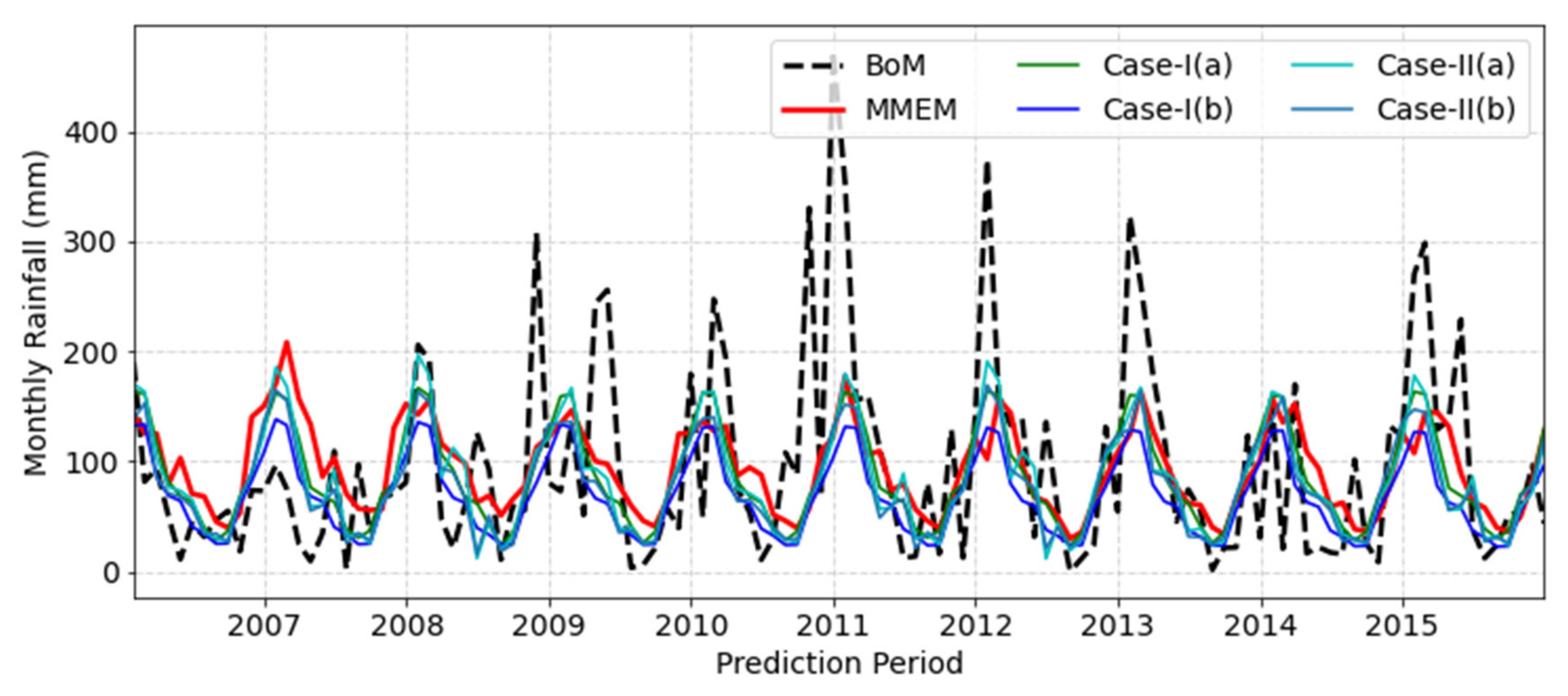
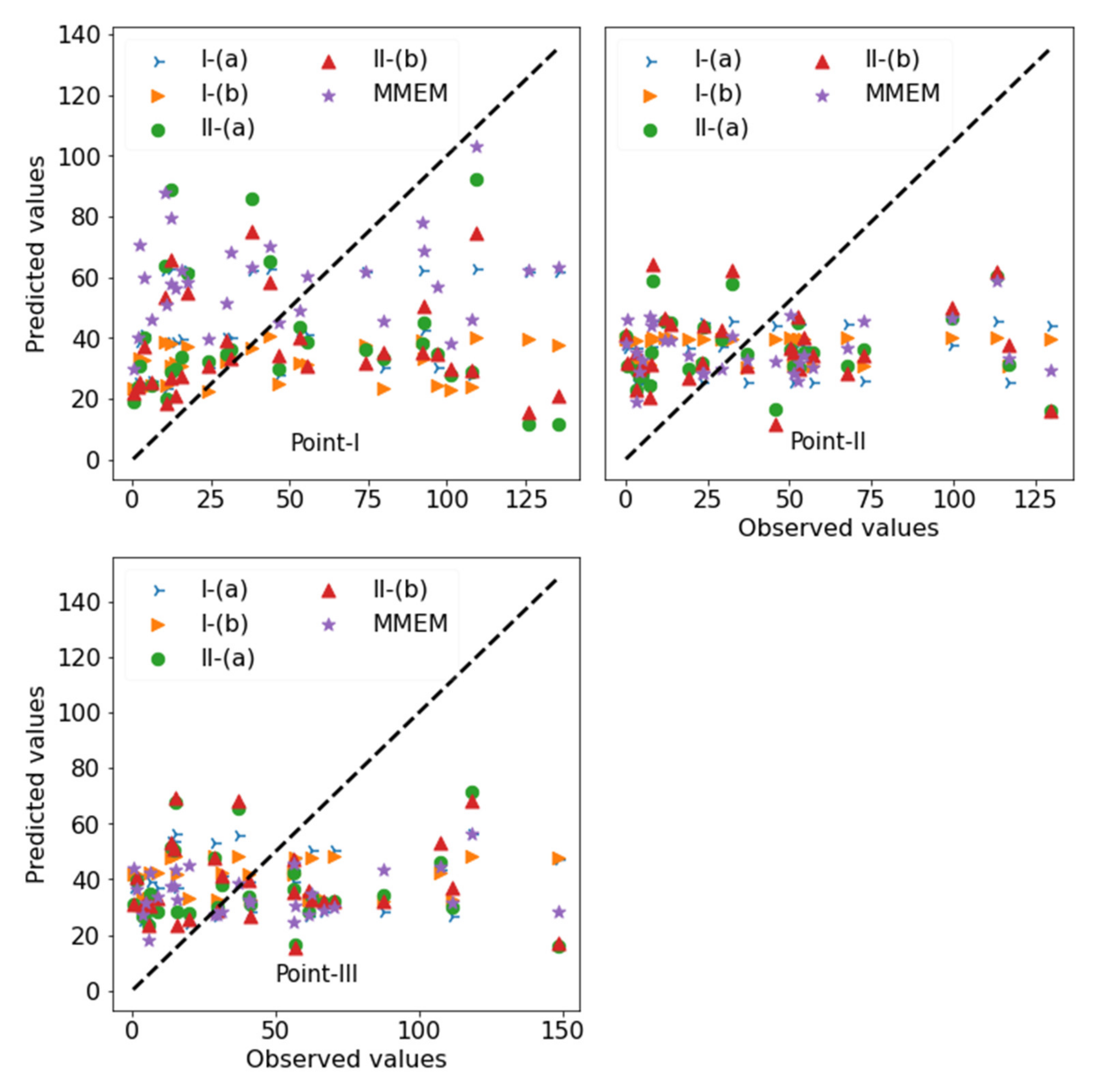
3.1. Prediction Using FBP

Figure 2 presents the comparison between observed and FBP-predicted monthly rainfall values of different cases at Point-I, where Case-I presents the data-driven approach, MMEM presents the knowledge-driven approach, and Case-II presents the combination of the knowledge and data-driven approaches. From the comparison, it is evident that FBP can reproduce seasonal variability with better performance when producing dry events, but none of the cases of FBP could reproduce the extreme peak values of the observed rainfall.
However, Case-II (a) showed comparatively better performance to catch the upper peaks, followed by Case-I (a). For the dry events, Case-II showed a considerably better resemblance with the observed values compared to Case-I. This means prediction skills improve, especially in dry events, when the combination of the knowledge and data-driven approaches is employed. These improvements were also observed in the skill tests of all considered cases. Table 2 presents the different skill test results and the percentage of over and under prediction of total rainfall, the cumulative sum over the different periods, and different cases of FBP along with MMEM at three selected points.
Comparing the predicted values and their skill tests at all three points, it is evident that Case-I (a) showed comparatively better skills and a lower percentage of under/over prediction of total rainfall than Case-I (b). This is due to the higher training period (1911–2015) of Case-I (a), which was about double the training period of all other cases. This means, with a higher training period, FBP can reach a better prediction performance. Among the cases of similar training periods, Case-II (a) showed comparatively better skill scores at Point-I where the FBP model parameter values were optimized. However, at points II and III, Case-II (b) showed higher skills than Case-II (a). The better performance of Case-II (b) may be due to the involvement of a range of climate responses provided by the different GCMs as individual regressors, or their higher skills than the MMEM. On the contrary, the better skills of Case-II (a) at Point-I may be either due to the better skills of the MMEM that guided FBP as an additional regressor, or the tuning of the FBP parameters (at the other two points, the FBP models’ parameter values were not tuned).
It is difficult to attach here any valid reason behind why Case-II (b) performed better in the other two points but not at Point-I, as no comparison was conducted during the performance of MMEM and all selected GCMs between the points. Anyway, Case-II (either a or b), as the combination of the knowledge and data-driven approaches, provided better prediction skills than only the data-driven approaches. From the predicted values and their skill comparisons at all three selected points, this study reveals that the skill improvement of FBP predictions with the combination of the knowledge and data-driven approaches was due to better capturing the dry events, and doing so even better than the MMEM (Figure 3). For reproducing the peak values (upper extremes), the knowledge-driven approach (MMEM) was found to be better than the FBP predictions. From Figure 3, it can be observed that, for the dry events (lower values), FBP predictions showed a comparatively better resemblance with the observed values and worse predictions for the upper peaks (wet events). For capturing the dry events, the combination of the knowledge and data-driven approaches was found to be better than any of the individual approaches; Case-II (b) was only slightly better than II (a) in terms of all tested skills, as well as total rainfall prediction over different time spans.

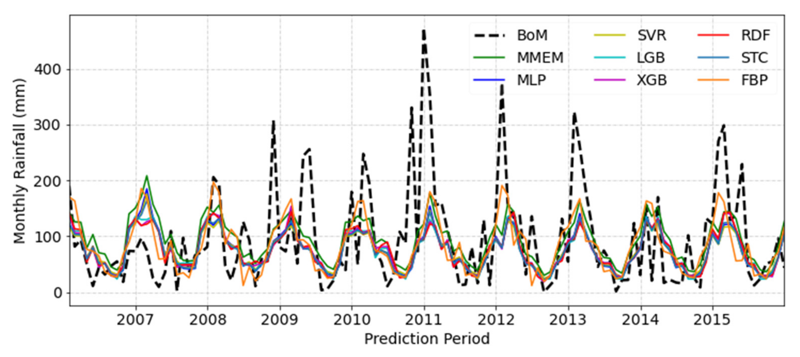
3.2. Prediction Using Regression Models

A comparison of monthly rainfall prediction at Point-I by five supervised machine learning regression algorithms and their stacking models (STC) using MMEM as the feature is presented in Figure 4. From the comparison, it can be observed that the regression models were also able to reproduce seasonal variations with very little improvement in reproducing the lower extremes compared to the MMEM. This study also used all selected models as independent variables, but the results were not as good as the MMEM. For this reason, only the skills of the regression models using MMEM as a feature are presented here. From the comparisons, it can be observed that all regression models, except RDF, showed similar skills in monthly rainfall prediction, among which MLP and SVR were comparatively better than the others (see Table 3). From the comparison of the predicted monthly rainfall values and the skills tests, this study finds that the regression models showed little improvement in reproducing the lower extremes compared to the MMEM, and the reverse in reproducing the peak values (upper extremes).
In reproducing the lower extremes, FBP showed better performance than the regression models, and this was the same even for the upper extremes. Note that the correction factors are employed in FBP predictions, but no such correction factors are considered for the regression models. However, the reason behind the better performance of FBP to catch the dry events could be due to employing the correction factor or due to choosing the multiplicative seasonality function, or a combination of both, enabling FBP to reproduce wider seasonal variation compared to the regression models [42]. The skill test results showed little weak prediction where IA values varied between 0.5 and 0.62, and MAE values varied between 40 and 50. The main reason behind these weak skills was that there were very frequent extreme peaks in the observed values (see Figure 2 or Figure 4) which were used to measure the skills. Another reason may be the comparatively shorter training period (1960–2005) where FBP was not familiar with the rainfall values above 250 mm for the target variable during the training process, as these were set to 250 mm to remove the outliers from the observed datasets.
Upon comparing Figure 3 and Figure 5, it can be seen that FBP and the regression models showed a comparatively better resemblance of the lower extreme values (dry events) than the MMEM. Note that GCMs are imperfect replicas of real-world phenomena and contain systematic biases [43]. They intend to overestimate the wet events and underestimate the dry events [44,45]. GCM outputs need rigorous correction before application [46,47,48,49]. This study reveals that rainfall prediction at the local level using FBP, using a combination of both GCMs and observed data, would enhance the overall prediction accuracy. A longer training period using a longer period of GCM-derived hindcast data may enable FBP to provide better skills in reproducing dry events, which was seen in the first case (Case-I). Note that this study used two different types of datasets (GCMs and observed) of the same time span and followed a supervised training approach where known observed values were used for both the training and the prediction period (for comparison with the predicted values). As no real future data were predicted here, one can consider the training period as verification and the assessed prediction skills as validation.
Every individual future prediction model, either an ANN or any ML algorithm, is different, and shows different performance depending on function, tuning parameters, and the variables considered for predictions. In addition, every individual precipitation time series is different at different geographical locations. For the prediction purpose, researchers used different models with different input variables and data pre-processing techniques. Then, performances were assessed based on the corresponding observed values. That is why it is difficult to compare and contrast different types of models for different regions and periods with the results obtained in this study.
The early prediction of upper and lower extremes can help in managing floods and droughts, respectively. However, in this study, it was observed that neither the FBP model nor the ML regression model could reproduce extreme wet events. Rather, they could reproduce the dry events considerably better than the wet events. Reproducing the dry events is also important to agriculture-dependent countries such as Australia, where the most variable climate exists. In Australia, a typical major drought in a season may reduce agricultural production by about 10% and gross national product by 1% [50]. This study will be beneficial for: water resource managers assessing future water availability; managing agriculture and agricultural-dependent businesses; and other water-related stakeholders planning and developing infrastructures.

4. Conclusions

Rainfall prediction is highly important from both social and economic perspectives. Predictions through GCMs and other time series models have been seen individually, but the application of GCM-derived precipitation together with observed values in a time series model on a decadal scale has not yet been found. On the contrary, as a relatively new time series forecasting library, the application of Facebook Prophet in rainfall prediction can hardly be found in the literature. For time series data, which have strong seasonality, Facebook Prophet works well for future prediction. As climate variables show seasonality over the cycle of a year, this study aimed to predict monthly rainfall using a combination of both GCM-derived and observed data through the Facebook Prophet model. In doing so, this study used historically observed monthly rainfall as the input and GCM-derived monthly precipitation from the CMIP5 decadal experiment as an additional regressor. Multiple additional regressors were implemented and compared with the performance of a single additional regressor. A few correction factors were introduced for the predicted values of different months that enabled FBP to provide better prediction accuracy. From the comparison of skills, this study finds that the combination of both GCM-derived and observed values gives better prediction accuracy compared to predictions based on the observed data only. Using GCM-derived data as an additional regressor guided the FBP model for future prediction. GCM-derived data includes not only scientific understanding, but also the historical records that guided FBP to come up with higher prediction accuracy. Based on the outlined skills assessments, the following conclusions are drawn.
(i)
FBP can reproduce dry events considerably better than wet events. This may be due to a better understanding of FBP of dry periods through the training and its multiplicative seasonality function;
(ii)
Following the combination of GCM-derived data (as an additional regressor) and the corresponding observed values, FBP should be able to reproduce future rainfall with higher prediction accuracy than the predictions based on the observed values only;
(iii)
A higher number of regressors will provide comparatively better prediction accuracy than a single additional regressor. In this case, a longer period of GCM hindcast data would elicit a higher prediction accuracy.
However, this study compared the performance of FBP with six regression models for the same places and same datasets, and found that FBP outperformed them. This study highly encourages the cross-validation of a similar approach by using different forms and architecture of deep ANNs that may increase prediction accuracy by utilizing different tuneable features.

Supplementary Materials

The following supporting information can be downloaded at: https://0-www-mdpi-com.brum.beds.ac.uk/article/10.3390/hydrology9060111/s1, Table S1. Regression models’ parameters and their most possible values used in this study.

Author Contributions

M.M.H., conceptualization, data curation, formal analysis, investigation, methodology, software, visualization, writing—original draft; A.H.M.F.A., conceptualization, funding acquisition, project administration, resources, supervision, writing—review and editing; N.G., data curation, investigation, software, validation, visualization, writing—review and editing; M.P., data curation, funding acquisition, project administration, resources, supervision, writing—review and editing; M.B., supervision, validation, writing—review and editing. All authors have read and agreed to the published version of the manuscript.

Funding

This research was jointly funded by CIPRS scholarship of Curtin University of Technology and Data61 student scholarship of CSIRO (Commonwealth Scientific and Industrial Research Organization) those were provided to the first author for his PhD study at Curtin University of Technology, Australia.

Institutional Review Board Statement

Not applicable.

Informed Consent Statement

Not applicable.

Data Availability Statement

This study used open access climate model data available at CMIP5 data portal (https://esgf-node.llnl.gov/projects/cmip5/, accessed on 20 June 2018). It is mentioned in Section 2.2. The details of the selected models is presented in Table 1. The processed and analyzed data will be stored in the research data repository of Curtin University, Western Australia. Data can be accessed through Curtin University after following its data sharing policy.

Acknowledgments

The authors are thankful to the working groups of the World Climate Research Program who made the CMIP5 decadal experiment data available for the researchers. Authors also would like to thank the Australian Bureau of Meteorology for providing the gridded observed rainfall data and the catchment’s shape file. Authors gratefully acknowledge the financial support from Curtin University, Perth, Australia and CSIRO Data61, Melbourne, Australia.

Conflicts of Interest

We, all authors, declare no conflict of interest and no financial issues relating to the submitted manuscript. We warrant that the article is the authors’ original work.

References

  1. Hansen, J.W.; Mason, S.J.; Sun, L.; Tall, A. Review of Seasonal Climate Forecasting for Agriculture in Sub-Saharan Africa. Exp. Agric. 2011, 47, 205–240. [Google Scholar] [CrossRef] [Green Version]
  2. Jones, J.; Hansen, J.; Royce, F.; Messina, C. Potential benefits of climate forecasting to agriculture. Agric. Ecosyst. Environ. 2000, 82, 169–184. [Google Scholar] [CrossRef]
  3. Mehta, V.M.; Knutson, C.L.; Rosenberg, N.J.; Olsen, J.; Wall, N.A.; Bernadt, T.K.; Hayes, M.J. Decadal Climate Information Needs of Stakeholders for Decision Support in Water and Agriculture Production Sectors: A Case Study in the Missouri River Basin. Weather Clim. Soc. 2013, 5, 27–42. [Google Scholar] [CrossRef] [Green Version]
  4. Apurv, T.; Mehrotra, R.; Sharma, A.; Goyal, M.K.; Dutta, S. Impact of climate change on floods in the Brahmaputra basin using CMIP5 decadal predictions. J. Hydrol. 2015, 527, 281–291. [Google Scholar] [CrossRef]
  5. Ouyang, Q.; Lu, W.; Xin, X.; Zhang, Y.; Cheng, W.; Yu, T. Monthly Rainfall Forecasting Using EEMD-SVR Based on Phase-Space Reconstruction. Water Resour. Manag. 2016, 30, 2311–2325. [Google Scholar] [CrossRef]
  6. Mislan; Haviluddin; Hardwinarto, S.; Sumaryono; Aipassa, M. Rainfall Monthly Prediction Based on Artificial Neural Network: A Case Study in Tenggarong Station, East Kalimantan-Indonesia. Procedia Comput. Sci. 2015, 59, 142–151. [Google Scholar] [CrossRef] [Green Version]
  7. George, J.; Janaki, L.; Gomathy, J.P. Statistical Downscaling Using Local Polynomial Regression for Rainfall Predictions—A Case Study. Water Resour. Manag. 2015, 30, 183–193. [Google Scholar] [CrossRef]
  8. Hung, N.Q.; Babel, M.S.; Weesakul, S.; Tripathi, N.K. An artificial neural network model for rainfall forecasting in Bangkok, Thailand. Hydrol. Earth Syst. Sci. 2009, 13, 1413–1425. [Google Scholar] [CrossRef] [Green Version]
  9. Mekanik, F.; Lee, T.S.; Imteaz, M.A. Rainfall Modeling Using Artificial Neural Network for a Mountainous Region in West Iran. In Proceedings of the 19th International Congress on Modelling and Simulation, Perth, Australia, 12–16 December 2011; pp. 3518–3524. [Google Scholar] [CrossRef]
  10. Ali, M.; Deo, R.C.; Downs, N.J.; Maraseni, T. Monthly rainfall forecasting with Markov Chain Monte Carlo simulations integrated with statistical bivariate copulas. In Handbook of Probabilistic Models; Butterworth-Heinemann: Oxford, UK, 2020; pp. 89–105. [Google Scholar] [CrossRef]
  11. Hossain, I.; Rasel, H.M.; Alam Imteaz, M.; Mekanik, F. Long-term seasonal rainfall forecasting using linear and non-linear modelling approaches: A case study for Western Australia. Arch. Meteorol. Geophys. Bioclimatol. Ser. B 2019, 132, 131–141. [Google Scholar] [CrossRef]
  12. Hong, W.-C. Rainfall forecasting by technological machine learning models. Appl. Math. Comput. 2008, 200, 41–57. [Google Scholar] [CrossRef]
  13. Rajeevan, M. Prediction of Indian Summer Monsoon: Status, Problems and Prospects. Curr. Sci. 2001, 81, 1451–1457. [Google Scholar]
  14. Zhang, G.P. Time series forecasting using a hybrid ARIMA and neural network model. Neurocomputing 2003, 50, 159–175. [Google Scholar] [CrossRef]
  15. Machiwal, D.; Jha, M.K. Hydrologic Time Series Analysis: Theory and Practice; Springer: Dordrecht, The Netherlands, 2012; ISBN 978-94-007-1861-6. [Google Scholar]
  16. Dastorani, M.; Mirzavand, M.; Dastorani, M.T.; Sadatinejad, S.J. Comparative study among different time series models applied to monthly rainfall forecasting in semi-arid climate condition. Nat. Hazards 2016, 81, 1811–1827. [Google Scholar] [CrossRef]
  17. Meinke, H.; Sivakumar, M.V.K.; Motha, R.P.; Nelson, R. Preface: Climate Predictions for Better Agricultural Risk Management. Aust. J. Agric. Res. 2007, 58, 935–938. [Google Scholar] [CrossRef]
  18. Lee, J.; Kim, C.-G.; Lee, J.E.; Kim, N.W.; Kim, H. Application of Artificial Neural Networks to Rainfall Forecasting in the Geum River Basin, Korea. Water 2018, 10, 1448. [Google Scholar] [CrossRef] [Green Version]
  19. Shen, S.-L.; Zhang, N.; Zhou, A.; Yin, Z.-Y. Enhancement of neural networks with an alternative activation function tanhLU. Expert Syst. Appl. 2022, 199, 117181. [Google Scholar] [CrossRef]
  20. Lin, S.-S.; Zhang, N.; Zhou, A.; Shen, S.-L. Time-series prediction of shield movement performance during tunneling based on hybrid model. Tunn. Undergr. Space Technol. 2021, 119, 104245. [Google Scholar] [CrossRef]
  21. Wu, X.; Hongxing, C.; Flitman, A.; Fengying, W.; Guolin, F. Forecasting Monsoon Precipitation Using Artificial Neural Networks. Adv. Atmos. Sci. 2001, 18, 950–958. [Google Scholar] [CrossRef]
  22. Chakraverty, S.; Gupta, P. Comparison of neural network configurations in the long-range forecast of southwest monsoon rainfall over India. Neural Comput. Appl. 2007, 17, 187–192. [Google Scholar] [CrossRef]
  23. Chattopadhyay, S.; Chattopadhyay, G. Comparative study among different neural net learning algorithms applied to rainfall time series. Meteorol. Appl. 2008, 15, 273–280. [Google Scholar] [CrossRef]
  24. Committee, A.S. of C. E. T. Artificial Neural Networks in Hydrology. II: Hydrologic Applications by the ASCE Task Committee on Application of Artificial Neural Networks in Hydrology. J. Hydrol. Eng. 2000, 5, 115–123. [Google Scholar]
  25. Ramírez, M.C.; Ferreira, N.J.; Velho, H.F.C. Linear and Nonlinear Statistical Downscaling for Rainfall Forecasting over Southeastern Brazil. Weather Forecast. 2006, 21, 969–989. [Google Scholar] [CrossRef]
  26. Khandelwal, I.; Adhikari, R.; Verma, G. Time Series Forecasting Using Hybrid ARIMA and ANN Models Based on DWT Decomposition. Procedia Comput. Sci. 2015, 48, 173–179. [Google Scholar] [CrossRef] [Green Version]
  27. Unnikrishnan, P.; Jothiprakash, V. Hybrid SSA-ARIMA-ANN Model for Forecasting Daily Rainfall. Water Resour. Manag. 2020, 34, 3609–3623. [Google Scholar] [CrossRef]
  28. Trejo, A.; Martín, M.J.; Gómez-Quintana, A.; Cava, R.; García-Parra, J.J.; Ramírez, M.R. Effect of slicing of top quality (Montanera) Iberian dry-cured chorizo on the stability to high pressure treatment and storage. J. Food Sci. 2021, 86, 1963–1978. [Google Scholar] [CrossRef]
  29. Toharudin, T.; Pontoh, R.S.; Caraka, R.E.; Zahroh, S.; Lee, Y.; Chen, R.C. Employing long short-term memory and Facebook prophet model in air temperature forecasting. Commun. Stat. Simul. Comput. 2021, 2021, 1854302. [Google Scholar] [CrossRef]
  30. Samal, K.K.R.; Babu, K.S.; Das, S.K.; Acharaya, A. Time Series based Air Pollution Forecasting using SARIMA and Prophet Model. In Proceedings of the 2019 International Conference on Information Technology and Computer Communications, Singapore, 16–18 August 2019; pp. 80–85. [Google Scholar] [CrossRef]
  31. Subashini, A.; K, S.; Saranya, S.; Harsha, U. Forecasting Website Traffic Using Prophet Time Series Model. Int. Res. J. Multidiscip. Technov. 2019, 1, 56–63. [Google Scholar] [CrossRef]
  32. Climate-Data. Brisbane Climate: Average Weather, Temperature, Rainfall. 2020. Available online: https://www.climatestotravel.com/climate/australia/brisbane (accessed on 25 March 2021).
  33. Australian Bureau of Meteorology (BoM). Annual Rainfall. State of the Environment (Department of Environment and Science). Queensland Government. 2020. Available online: https://www.stateoftheenvironment.des.qld.gov.au/climate/climate-observations/annual-rainfall (accessed on 21 July 2021).
  34. Frost, A.J.; Ramchurn, A.; Smith, A. The Bureau ’s Operational AWRA Landscape (AWRA-L) Model; Technical Report; Bureau of Meteorology (BoM): Melbourne, Australia, 2016. [Google Scholar]
  35. Jones, P.W. First- and Second-Order Conservative Remapping Schemes for Grids in Spherical Coordinates. Mon. Weather Rev. 1999, 127, 2204–2210. [Google Scholar] [CrossRef]
  36. Hossain, M.M.; Garg, N.; Anwar, A.H.M.F.; Prakash, M. Comparing Spatial Interpolation Methods for CMIP5 Monthly Precipitation at Catchment Scale. Indian Water Resour. Soc. 2021, 41, 28–34. [Google Scholar]
  37. Taylor, S.J.; Letham, B. Forecasting at Scale. Am. Stat. 2018, 72, 37–45. [Google Scholar] [CrossRef]
  38. Hossain, M.M.; Anwar, A.H.M.F.; Garg, N.; Prakash, M.; Bari, M. Evaluation of CMIP5 Decadal Precipitation at Catchment Level. Int. J. Climatol. 2022. under-review. [Google Scholar]
  39. Hossain, M.; Garg, N.; Anwar, A.H.M.F.; Prakash, M.; Bari, M. Intercomparison of drift correction alternatives for CMIP5 decadal precipitation. Int. J. Clim. 2021, 42, 1015–1037. [Google Scholar] [CrossRef]
  40. Wilks, D.S. Statistical Methods in the Atmospheric Sciences, 3rd ed.; Volume 100 (International Geophysics); Academic Press: Cambridge, MA, USA, 2011. [Google Scholar]
  41. Wilmot, C.J. Some Comments on the Evaluation of Model Performance. Bull. Am. Meteorol. Soc. 1982, 63, 1309–1313. [Google Scholar] [CrossRef] [Green Version]
  42. Kourentzes, N. Additive and Multiplicative Seasonality—Can You Identify Them Correctly? 2014. Available online: https://kourentzes.com/forecasting/2014/11/09/additive-and-multiplicative-seasonality/ (accessed on 4 August 2021).
  43. Randall, D.A.; Wood, R.A.; Bony, S.; Colman, R.; Fichefet, T.; Fyfe, J.; Kattsov, V.; Pitman, A.; Shukla, J.; Srinivasan, J.; et al. Climate Models and Their Evaluation. In Climate Change 2007: The Physical Science Basis; Contribution of Working Group I to the Fourth Assessment Report of the IPCC (FAR); Cambridge University Press: Cambridge, UK, 2007; pp. 589–662. [Google Scholar]
  44. Sun, Y.; Solomon, S.; Dai, A.; Portmann, R. How Often Will It Rain? J. Clim. 2007, 20, 4801–4818. [Google Scholar] [CrossRef]
  45. Stephens, G.L.; L ’Ecuyer, T.; Forbes, R.; Gettelmen, A.; Golaz, J.-C.; Bodas-Salcedo, A.; Suzuki, K.; Gabriel, P.; Haynes, J. Dreary state of precipitation in global models. J. Geophys. Res. Earth Surf. 2010, 115, 014532. [Google Scholar] [CrossRef]
  46. Islam, S.A.; Bari, M.; Anwar, A.H.M.F. Assessment of Hydrologic Impact of Climate Change on Ord River Catchment of Western Australia for Water Resources Planning: A Multi-Model Ensemble Approach. In Proceedings of the 19th International Congress on Modelling and Simulation, Perth, Australia, 12–16 December 2011. [Google Scholar] [CrossRef]
  47. Islam, S.A.; Bari, M.A.; Anwar, A.H.M.F. Hydrologic impact of climate change on Murray–Hotham catchment of Western Australia: A projection of rainfall–runoff for future water resources planning. Hydrol. Earth Syst. Sci. 2014, 18, 3591–3614. [Google Scholar] [CrossRef] [Green Version]
  48. Maurer, E.P.; Hidalgo, H.G. Utility of daily vs. monthly large-scale climate data: An intercomparison of two statistical downscaling methods. Hydrol. Earth Syst. Sci. 2008, 12, 551–563. [Google Scholar] [CrossRef] [Green Version]
  49. Mehrotra, R.; Sharma, A. Development and Application of a Multisite Rainfall Stochastic Downscaling Framework for Climate Change Impact Assessment. Water Resour. Res. 2010, 46, 008423. [Google Scholar] [CrossRef]
  50. White, B. The Importance of Climate Variability and Seasonal Forecasting to the Australian Economy. In Applications of Seasonal Climate Forecasting in Agricultural and Natural Ecosystems; Hammer, G.L., Nicholls, N., Mitchell, C., Eds.; Springer: Dordrecht, The Netherlands, 2000; Volume 21, pp. 1–22. [Google Scholar] [CrossRef]
Figure 1. Study area.
Hydrology 09 00111 g001
Figure 2. Comparison of FBP-predicted monthly rainfall of different cases with the corresponding observed values.
Hydrology 09 00111 g002
Figure 3. Comparison of the resemblance of dry and wet events produced by FBP and MMEM.
Hydrology 09 00111 g003
Figure 4. Monthly rainfall predicted from different regression models.
Hydrology 09 00111 g004
Figure 5. Comparison of the resemblance of dry and wet events produced by regression models.
Hydrology 09 00111 g005
Table 1. List of models (GCMs) used as additional regressors in this study.
Modelling Centre
(or Group)
Resolutions
(Lon × Lat)
Initialization Year (1960–2005)
60657075808590950005
Number of Ensembles
EC-EARTH(1.125 × 1.1215)14141414141414141018
MRI-CGCM3(1.125 × 1.1215)06080909060909090906
MPI-ESM-LR(1.875 × 1.865)10101010101010101010
MPI-ESM-MR(1.875 × 1.865)03030303030303030303
MIROC4h(0.5625 × 0.5616)03030306060606060606
MIROC5(1.4062 × 1.4007)06060606040606060606
CanCM4(2.8125 × 2.7905)20202020202020202020
CMCC-CM(0.75 × 0.748)03030303030303030303
Table 2. Comparison of skills and total rainfall prediction among the different cases of FBP models.
Location (Lon/Lat)CasesSkillsUnder and Overestimation of Total Rainfall (%)
MAEPCCACCIA1Y3Y5Y8Y
Point-I (153.05 E/27.50 S)I-(a)53.60.5490.5360.61535.914.6−7.2−11.2
I-(b)55.90.5260.4180.49111.9−5.94−24.6−28.7
II-(a)54.90.5330.5170.62233.515.1−8.34−12.8
II-(b)55.10.5280.4880.57724.85.25−16.0−19.3
MMEM58.110.4340.4330.51048.635.65.64−3.1
Point-II (152.0 E/27.0 S)I-(a)40.80.4970.4960.60350.226.52.12−10.4
I-(b)41.00.4840.4840.58150.727.12.46−6.4
II-(a)40.80.4890.4860.59347.326.30.53−8.4
II-(b)39.80.5190.5170.61138.522.7−1.42−8.2
MMEM41.40.4940.4930.61258.239.313.8−5.6
Point-III (152.05 E/27.30 S)I-(a)46.10..4910.4900.58854.424.13.4−6.7
I-(b)48.10.4710.4700.58365.532.110.6−0.15
II-(a)46.90.4640.4600.56751.723.11.1−9.9
II-(b)45.20.4900.4850.58044.618.7−1.6−10.2
MMEM44.70.4890.4740.57148.723.9−0.8−14.2
Table 3. Skills comparison of different regression models.
ModelsPoint-IPoint-IIPoint-III
MAEPCCACCIAMAEPCCACCIAMAEPCCACCIA
MLP57.10.4300.3710.44539.30.4800.4500.51543.50.4760.4270.494
SVR57.60.4300.3610.41839.30.4810.4470.51643.50.4780.4300.487
LGB56.60.4320.3740.44239.50.4690.4320.51043.70.4660.4250.493
XGB57.20.4270.3700.43939.70.4510.4170.50344.10.4440.4100.484
RDF57.20.4260.3690.44139.90.4270.3720.43344.00.4210.3590.412
STC57.10.4340.3650.43539.10.4830.4250.47543.40.4640.4050.464
FBP(II-a)54.90.5330.5170.62240.90.4890.4860.59346.90.4640.4600.567
MMEM58.10.4340.4330.51041.40.4940.4930.61244.70.4890.4740.571
Publisher’s Note: MDPI stays neutral with regard to jurisdictional claims in published maps and institutional affiliations.

