
Assessment of Deep Convective Systems in the Colombian Andean Region

IIHR Hydroscience & Engineering, Iowa Flood Center, The University of Iowa, Iowa City, IA 52240, USA
Hydrology 2022, 9(7), 119; https://0-doi-org.brum.beds.ac.uk/10.3390/hydrology9070119
Submission received: 12 May 2022
/
Revised: 10 June 2022
/
Accepted: 20 June 2022
/
Published: 28 June 2022
(This article belongs to the Special Issue Advances in Modelling of Rainfall Fields)
Abstract
:In tropical regions, deep convective systems are associated with extreme rainfall storms that usually detonate flash floods and landslides in the Andean Colombian region. Several studies have used satellite data to address the structure and formation of tropical convective storms. However, there is a local gap in the characterization, which is essential for a better understanding of flash floods and preparedness, filling a gap in a region with scarce information regarding extreme events. In this work, we assess the deep convective storms in a mountainous region of Colombia using meteorological radar observations between 2014 and 2017. We start by identifying convective and stratiform formations. We refine the convective identification by classifying convective systems into enveloped (contained in a stratiform system) and unenveloped (not contained). Then, we analyze the systems’ temporal and spatial distributions and contrast them with the watersheds’ features. According to our results, unenveloped convective systems have higher reflectivity and hence higher rainfall intensities. Moreover, they also have a well-defined spatial and temporal distribution and are likely to occur in watersheds with elevation gradients of around 2000 and an aspect contrary to the wind direction. Our assessment of the convective storms is of significant value for the hydrologic community working on flash floods. Moreover, the spatiotemporal description is highly relevant for stakeholders and future local analysis.
1. Introduction
Convective systems usually turn into intense storms that could develop flooding events. Moreover, in regions with a steep terrain, convective storms are linked to the occurrence of flash floods [1,2,3,4], which are likely to produce human and infrastructure losses [5,6]. At the mesoscale, convective systems cover areas of around 600 [7], but it can be smaller at a local scale. Moreover, convective-detonated flash floods are usually limited to small catchments (less than 1000 ) [8,9,10] and their effects have been described in different world regions [9,11,12]. Nevertheless, there is a lack of analysis in the tropical Andean region, where topography-driven convective storms detonate shallow landslides and flash floods [13,14].
Several authors have described how the topography is intertwined with the occurrence of convective storms [15,16,17,18], with evidence of a strong connection [19,20,21,22]. Additionally, the described topographical influence increases with the elevation [23,24] and the aspect of the hillslopes relative to the preferential wind direction [24,25,26,27]. However, most of the work has been conducted in the Himalayas [7,23,28,29,30], the US [31,32], and in the southern Andean region [21,33,34]. Therefore, additional work is needed to understand the connection of the topography-convective system in the tropical Andes, specifically in the Colombian Andean region.
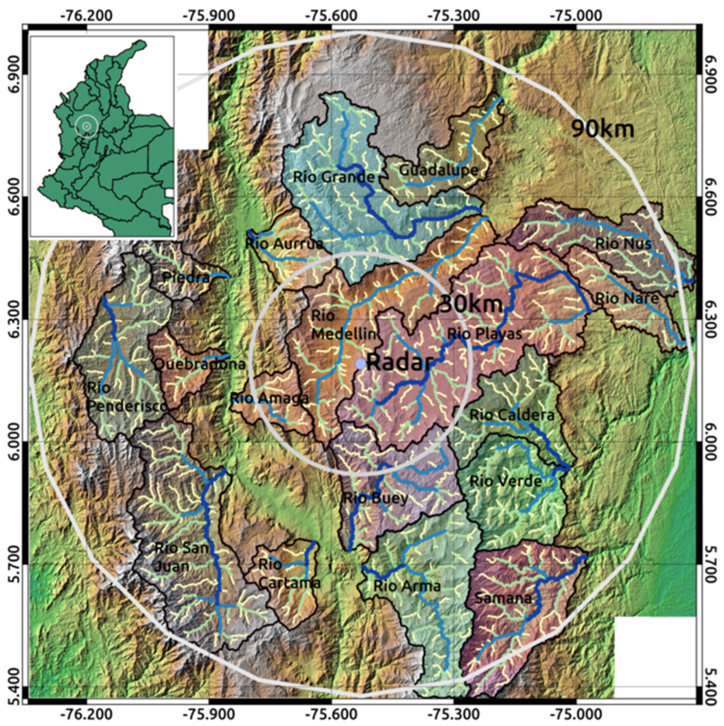
The Colombian Andean is made up of three mountainous rages, with its Weatherbeing dominated by the Intertropical Convergence Zone (ITCZ), the El Niño Southern Oscillation (ENSO), and the Pacific and Atlantic oceans’ oscillations [35,36,37]. The ITCZ develops two wet periods with higher rainfall accumulation (March to May and September to November) [38]. In addition, the La Niña phase of the ENSO usually increases the occurrence of convective storms [35] with significant socioeconomic impacts [39]. Nevertheless, there is a gap in the literature exploring convective systems and their connections with the topography. Most of the work conducted around the topic has been performed at a mesoscale using TRMM data [40,41], which has a coarse resolution in contrast with the local processes. However, local radar data improve the analysis resolution [31,42,43]. In the case of the Colombian Andean region, meteorological radar information became available in 2012 in the surroundings of the city of Medellin (see Figure 1). However, the continuity and quality of the data improved near the end of 2013.
This work uses local meteorological radar data to assess convective systems in the central Colombian Andean region between 2014 and 2017. Some of these convective systems detonated flash floods and landslides during this period [13,14]. First, we identify the stratiform and convective systems observed. Then, we classify the convective systems into enveloped and unenveloped, allowing us to describe the most intense ones better. We analyze the convective systems’ size, reflectivity, and spatial and temporal occurrences using radar data acquired by the Sistema de Alertas Tempranas Ambientales (SIATA). Additionally, we compare the localization of the identified convective systems with 18 watersheds. In the comparison, we explore how the aspect and elevation gradient of the watersheds are intertwined with the convective systems’ formation. Our main goal is to develop a comprehensive regional analysis of the storms linked to the occurrence of rainfall-related catastrophes in the Colombian Andean region. Additionally, we seek to fill a knowledge gap in a relevant topic that could worsen in the coming years due to climate change and population growth.
We begin this paper by describing the radar and topographic data in Section 2. Then, in the methodology Section 3, we describe the algorithms to identify convective systems, extract their features, and the methodology followed to contrast them against the selected watersheds. In Section 4, we present the results of the convective systems’ identification and the comparison with the watersheds. Finally, Section 5 offers our conclusions and remarks for future work.
2. Data and Information
We used radar reflectivity, digital elevation data, and wind data. Using radar reflectivity, we identified and analyzed the convective systems. Moreover, we delineated the watersheds and extracted their properties using a digital elevation model. Subsequently, we describe in detail the data used.
2.1. Radar Data
The polarimetric 350 Kw Doppler C-band radar manufactured by Enterprise Electronics Corporation is in the occidental central hill of the Aburra Valley watershed (Rio Medellin in Figure 1). The radar operation includes four plan position indicator sweeps (PPIs) at 0.5, 1.0, 2.0, and 4.0°. We used radar reflectivity every 5 min at the PPI of 1.0° with a Cartesian projected resolution of 128 . The radar beam has a beam width of 1°, and, depending on the PPI, it reaches a distance between 50 and 200 . It has a wavelength of 5.3 cm and an antenna gain of 45 dBZ. However, to avoid issues due to the bright band interception, we limited the information to a radius of 90 (second gray ring in Figure 1).
Radar data have been available since 2012. However, it has continuous quality data since 2014. The radar image quality control uses the co-polar correlation coefficient (CC). CC tends towards one when water particles have a uniform distribution. On the other hand, CC decreases when there is a heterogeneous distribution of the particles’ shape and orientation. Moreover, CC values above one represents errors due to noise. Between 2014 and 2017, around 93% of the radar data has a good quality.
2.2. Topography and Wind Data
We used an ALOS-PALSAR digital elevation model (DEM) to describe the region’s topography with a resolution of 12.7 m. Considering the area of the study domain, we resampled the DEM to a resolution of 40 m (background in Figure 1). We applied the algorithm [44] over the resampled DEM to estimate the direction map (DIR). Using the DEM and DIR maps, we extracted the watersheds shown in Figure 1 and their respective boundary sub-watersheds of orders 3, 4, and 5. Additionally, for each watershed, we estimated the total area, the elevation difference, and the predominant aspect. We used the watershed modeling framework (WMF) (https://github.com/nicolas998/WMF accessed on 12 May 2022) to perform the watershed delineation and analysis.
Additionally, we used ERA-5 observations at 750 to determine the preferential wind direction. The selected pressure level was around 2500 m above sea level, a value close to the mean elevation of the region.
3. Methodology
The region’s mountainous terrain induced extra challenges in our convective system assessment. Hillslopes with high elevation gradients promoted the formation of deep convective systems and, at the time, added noise to the radar images [45,46], increasing the uncertainty in the classification. Therefore, we divided the convective systems into two categories: enveloped and unenveloped. Enveloped systems are embedded into a stratiform formation, while unenveloped ones are not. With the convective discretization, we performed a more comprehensive assessment.
Additionally, we explored the relationship between convective systems’ spatial distribution and the topography. To this end, we delineated 18 watersheds (see Figure 1) and their boundary sub-watersheds with Horton orders 3, 4, and 5. Boundary sub-watersheds share a boundary with their containing watersheds. We measured the overlap between the convective systems and the watersheds and contrasted it with their area, aspect, and elevation difference. In this analysis, we also included the preferential direction of the wind near an elevation of 2500 m.
Subsequently, we describe in detail each one of the methodology steps.
3.1. Systems’ Classification and Analysis
We first identified the convective systems present in each radar image between 2014 and 2017. To perform the identification, we implemented in Fortran90 and Python the algorithm proposed by [47], and then modified by [48]. We also included functions to measure the features of the convective systems and classified them into enveloped and unenveloped. The code used can be found at the following GitHub repository: https://github.com/nicolas998/Radar (accessed on 12 May 2022).
3.1.1. Convective and Stratiform Systems’ Classifications
Convective storms exhibit high reflectivity and are prone to develop extreme rainfall events. On the other hand, stratiform formations have lower reflectivity and are associated with low-intensity rainfall. Considering the described differences, we started by separating convective and stratiform systems using the algorithm proposed by [47], and then modified by [48]. In our implementation, we used a background radius of 11 and a threshold for peaks of 40 dBZ. We validated the algorithm’s accuracy by comparing the classified systems with vertical profiles obtained by the radar [13]. Nevertheless, we identified noise due to convective systems embedded in stratiform formations. Therefore, we created the enveloped and unenveloped convective categories.
3.1.2. Enveloped and Unenveloped Convective Systems
Depending on the meteorological conditions and the temporal evolution of the storm, convective systems may occur as individual systems or as part of a cluster [49]. Single storms usually cover more area and have higher reflectivity than clustered systems. Moreover, during the storm, clustered systems are generally enveloped by a stratiform formation [50,51]. Therefore, we categorized convective systems into enveloped and unenveloped. Enveloped systems are embedded into stratiform formations, while unenveloped ones are not. We implemented the following procedures to identify both:
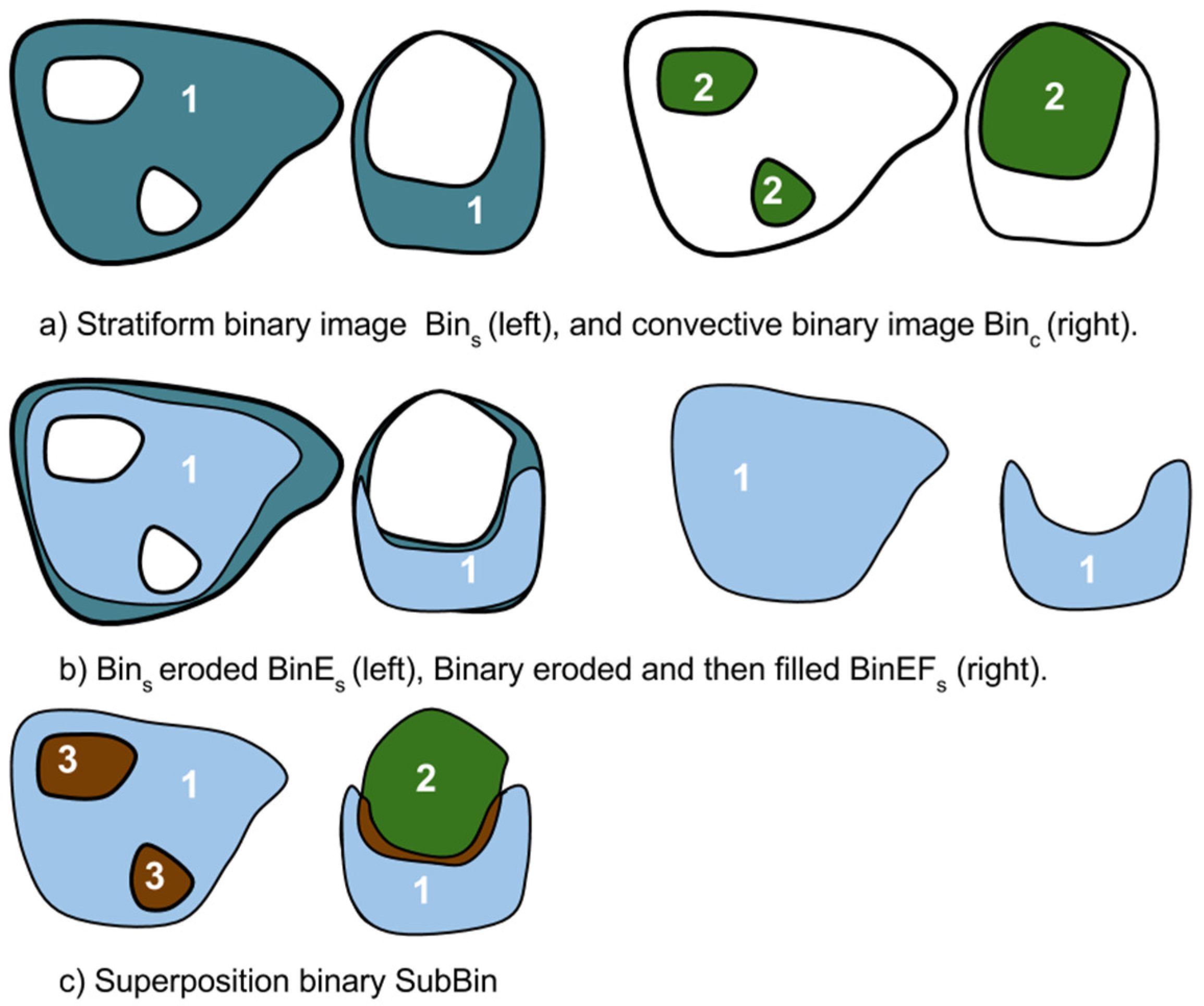
- First, we separated convective and stratiform objects into two binary images ( and , respectively). is equal to one where there are stratiform formations and zero elsewhere. is equal to two in regions with convective systems and zero elsewhere. Figure 2a presents a schematic of (left) and (right).
- Then, we eroded using a 3 × 3 kernel. In the erosion, each element with a value of one and at least one neighbor equal to zero in the kernel became zero. From the erosion, we obtained (light blue image in the left panel in Figure 2b).
- After the erosion, we filled the holes left in . From this procedure, we obtained the eroded and then filled stratiform binary (Figure 2b, right).
- Then, we computed the superposition between and as (Figure 2c). In , values equal to 1 correspond to stratiform formations, 2 to unenveloped convective systems, and 3 to enveloped convective systems.
- Finally, we classified each convective system as enveloped or unenveloped using their corresponding modal values in . For example, if 90 pixels of a convective storm were 2 and 10 pixels were 3, the system was considered unenveloped (or 2).
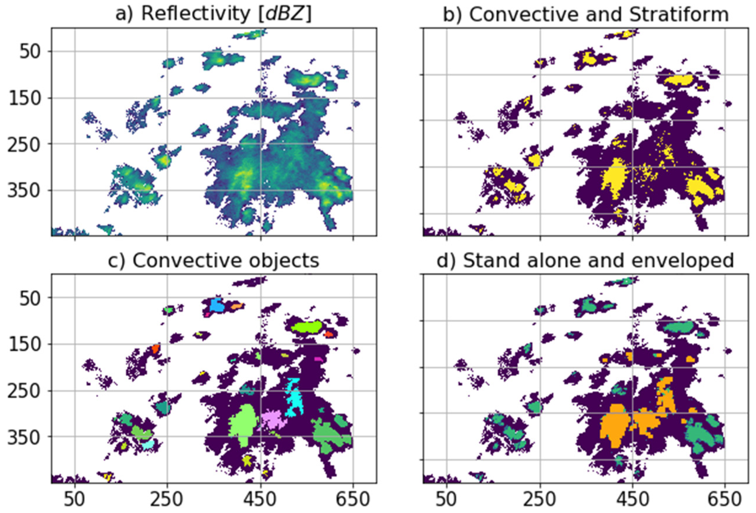
The described methodology was applied to each radar image. In Figure 3, we present an example showing the results obtained. The process starts with the reflectivity information (Figure 3a), from where we performed the convective and stratiform classifications (Figure 3b). Then, we identified each convective object (Figure 3c). An object is formed by all the adjacent pixels previously identified as convective. Finally, we obtained the enveloped and unenveloped convective systems’ identification (Figure 3d).
3.1.3. Reflectivity Statistics and Morphometrics
Using the described methodology, we processed the radar images between 2014 and 2017, obtaining a classified image every 5 min. We obtained a collection of convective objects (systems) from the classification. Then, we extracted the reflectivity statistics and morphometric features of each object. We used the equivalent reflectivity factor to compute the mean, , and deviation, , of each system, and transformed them to reflectivity by using their logarithm. Additionally, we computed the area, , the centroid coordinates, , and the time of occurrence of each convective system. The area corresponded to the pixel count in a system multiplied by 16,684 (the square of , the radar resolution), and the centroid was the system center of mass in X and Y. Moreover, we marked each object as enveloped (3) or unenveloped (2).
The described information allowed us to obtain an extensive collection of data and perform a comprehensive assessment of the convective systems in the region.
3.2. Watersheds Analysis
According to several studies, convective system formation is intertwined with topography [20,32]. The connection has also been reported in tropical regions [17,22] with links between rainfall rates and elevation [18,40]. However, most of the work used mesoscale information and did not consider the characteristics of the watersheds. Therefore, we compared the convective system localization with features of the watersheds in the region.
We analyzed the 18 watersheds delimited by the black divisor lines in Figure 1, covering most of the domain. The areas of the watersheds oscillated between 230 and 2000 , and the Horton stream orders at their outlets oscillated between 5 and 7. Additionally, we included the boundary sub-watersheds of the 18 watersheds with orders 3, 4, and 5 (see Figure 4a–c). A boundary sub-watershed has no upstream tributaries; in most cases, it shares its divisor line with its containing watershed. Then, we computed the following features of the watersheds: boundary elevation, maximum elevation gradient, predominant aspect (direction), and the upstream area [].
We also measured the intersection between the convective systems and the watersheds using the overlap index, , as follows:
where is the intersected area between the convective system and the watershed and is the system area. Figure 4d presents three different cases of overlap: There is no overlap when the convective system falls outside of a watershed and becomes equal to zero. There is a weak overlap when is less than 15% of the total area, and it is strong when is greater than 15%. Nevertheless, the described categories are subjective and will change depending on the watershed area and the resolution of the images used. Therefore, the given values are a reference that allows us to contrast the overlap between the convective systems and the watersheds.
Finally, we compared with the described features of the watersheds and the direction of the wind at 750 (ERA-5 data). Using the described procedure, we explored how the topographical features of the watersheds were intertwined with the occurrence of deep convective systems at different scales.
4. Results and Discussion
The main goal of our work was to present a characterization of the tropical convective systems observed by a meteorological radar. We also contrasted the convective systems with the region’s orientation, elevation, and aspects of several watersheds. We presented and discussed the obtained results after applying the methods described in Section 3.
4.1. Convective Systems Analyses
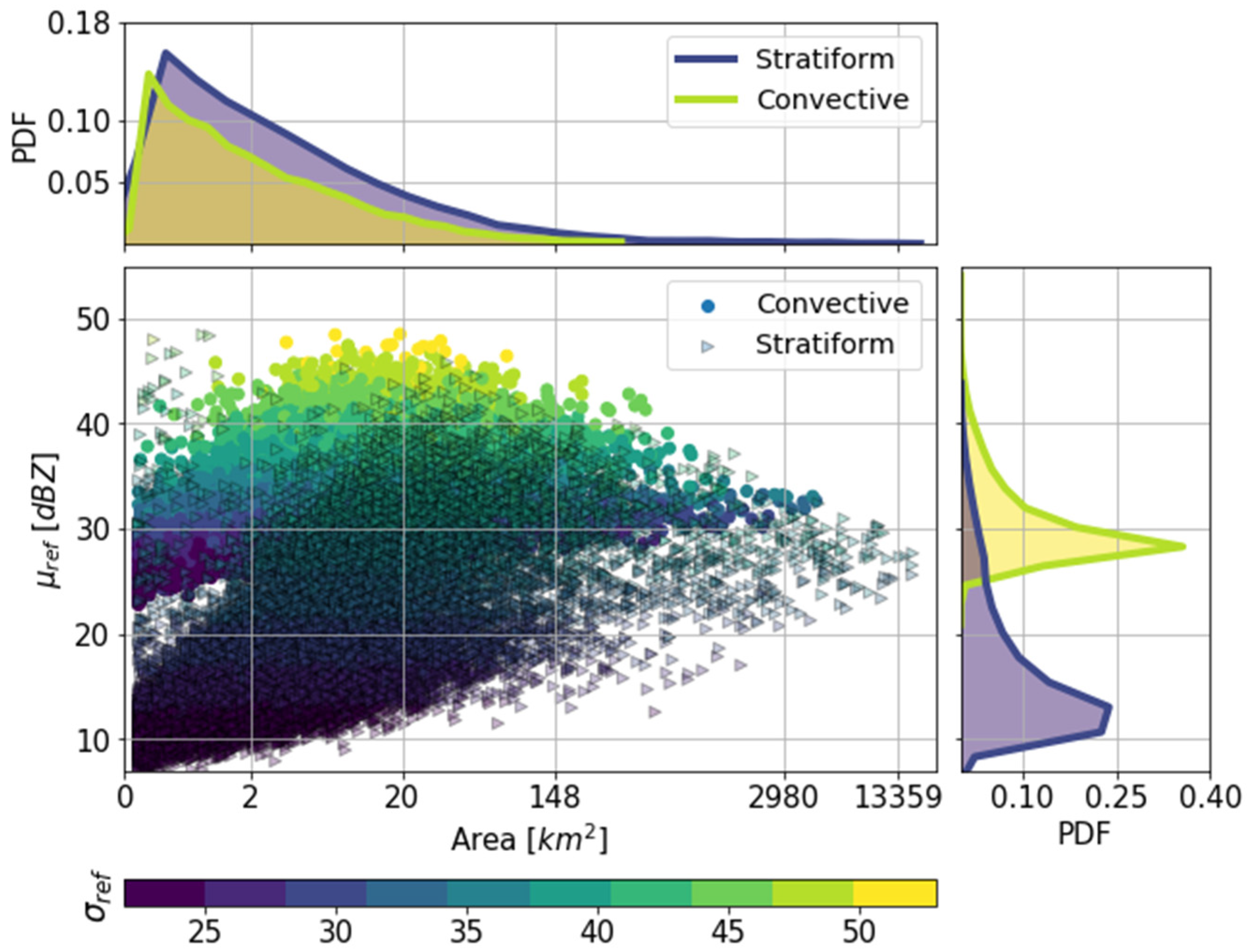
We started by identifying the observed convective and stratiform systems following the method proposed by Steiner (1995). Figure 5 presents the area, (X axis), mean reflectivity, (Y axis), and reflectivity deviation, (colors), of both kind of systems for a sample of 10,000 elements. According to it, the mean reflectivity distribution was different for the convective and stratiform systems. Convective distribution (green line in the vertical pdf panel) was less skewed and centered around 27 . On the other hand, the stratiform pdf (purple line) was skewed and centered around 12 . We also observed some differences in the distributions of their areas (top pdf panel). While stratiform areas oscillated around 0.01 and 13,000 with 80% below 40 , convective systems oscillated between 0.01 and 80 with 80% below 9 .
Convective and stratiform systems’ reflectivity statistics changed with the area of the system. For large areas, convective tended towards 30 while the stratiform towards 25 . Additionally, for areas around 20 , the convective and reached their maximum values of 48 and 50 , respectively. Moreover, the stratiform maximized for areas around 50 . In both cases, the mean reflectivity decreased for systems with areas below or above the ones mentioned. The described result may be related to the size of the watersheds where flash floods usually occur (areas below 100 ). According to the convective vs. area scatter in Figure 5, extensive convective system usually had a lower .
By comparing the area and distributions, we observed many relatively small convective systems with reduced reflectivity. The described pattern is also similar in the case of the stratiform systems. Both cases are likely attributed to misclassification caused by noise in the radar images. Therefore, we improved our classification by dividing the convective systems into two categories.
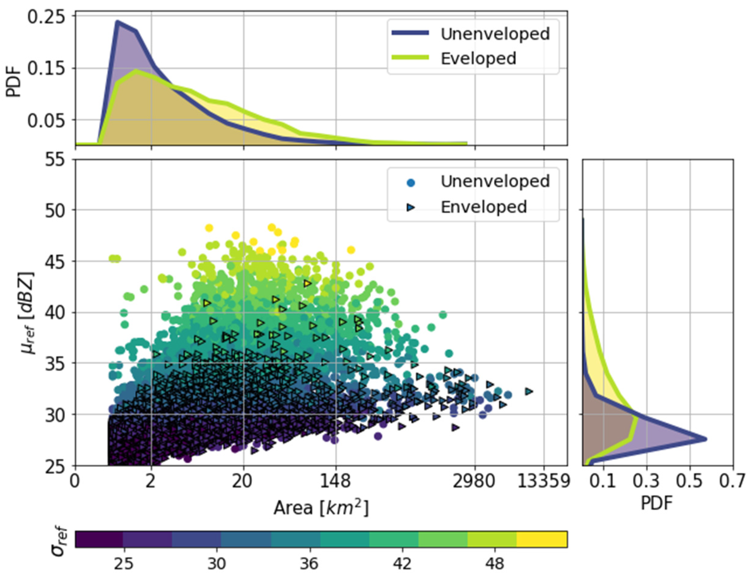
Using the methodology described in sub-Section 3.1.2, we classified 80% of the systems as unenveloped and 20% as enveloped. Figure 6 compares the area and of the enveloped (triangles) and unenveloped (circles) systems. Compared with Figure 5, the enveloped and unenveloped systems’ area and reflectivity are more similar. The mean reflectivity distributions of the enveloped and unenveloped categories were 28 and 32 , and the areas had mean values of 15 and 30 , respectively. Moreover, the unenveloped convective system’s was higher and peaked along with for systems with areas between 20 and 40 . Furthermore, the expected value of the unenveloped was considerably higher than the enveloped system (see Figure 6).
Table 1 summarizes the statistics of the stratiform, convective, enveloped, and unenveloped systems. According to the results, stratiform systems have an area with greater mean and deviation values. However, they have a lower mean reflectivity. On the other hand, convective systems have an area that oscillates around 24 . Enveloped systems are smaller and have a reflectivity lower than unenveloped systems. The described results mark the differences between both types of convective systems, highlighting unenveloped ones as good descriptors of deep convective systems. Moreover, our results also match the given description of convective clusters enveloped in stratiform formations [52].
The defined convective categories help us explore the region’s storm systems. Moreover, the studied features of both classes have relevant differences. Considering the described differences between the enveloped and unenveloped systems, we also explored their spatial and temporal differences.
4.2. Spatiotemporal Behavior
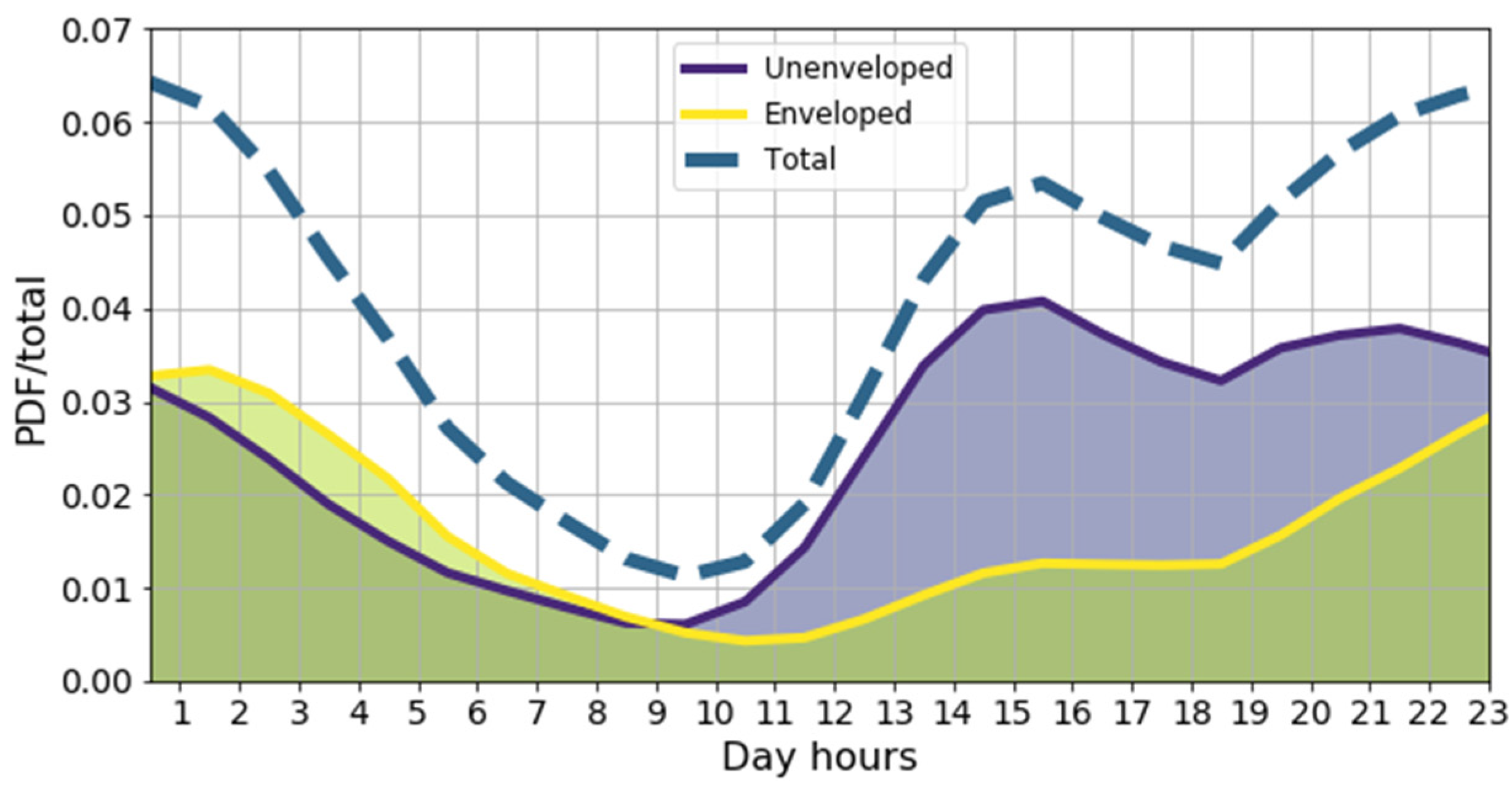
We first analyzed the convective systems’ diurnal and spatial distributions. We counted the hour of the day and the spatial localization of the convective, enveloped, and unenveloped systems. Then, we divided each count by the total of observed systems obtaining their probability of occurrence. Figure 7 presents the daily distribution observed in the region, starting at midnight and ending at 23:00. According to the figure, convective and undeveloped systems develop around noon, reaching the peak probability between 15:00 and midnight. On the other hand, enveloped systems are more likely to occur late at night and early morning. We attributed the observed temporal oscillations to surface heating and the eventual deep convection. Moreover, the increase in enveloped systems during the morning might be explained by the late stage of the deep convective systems.
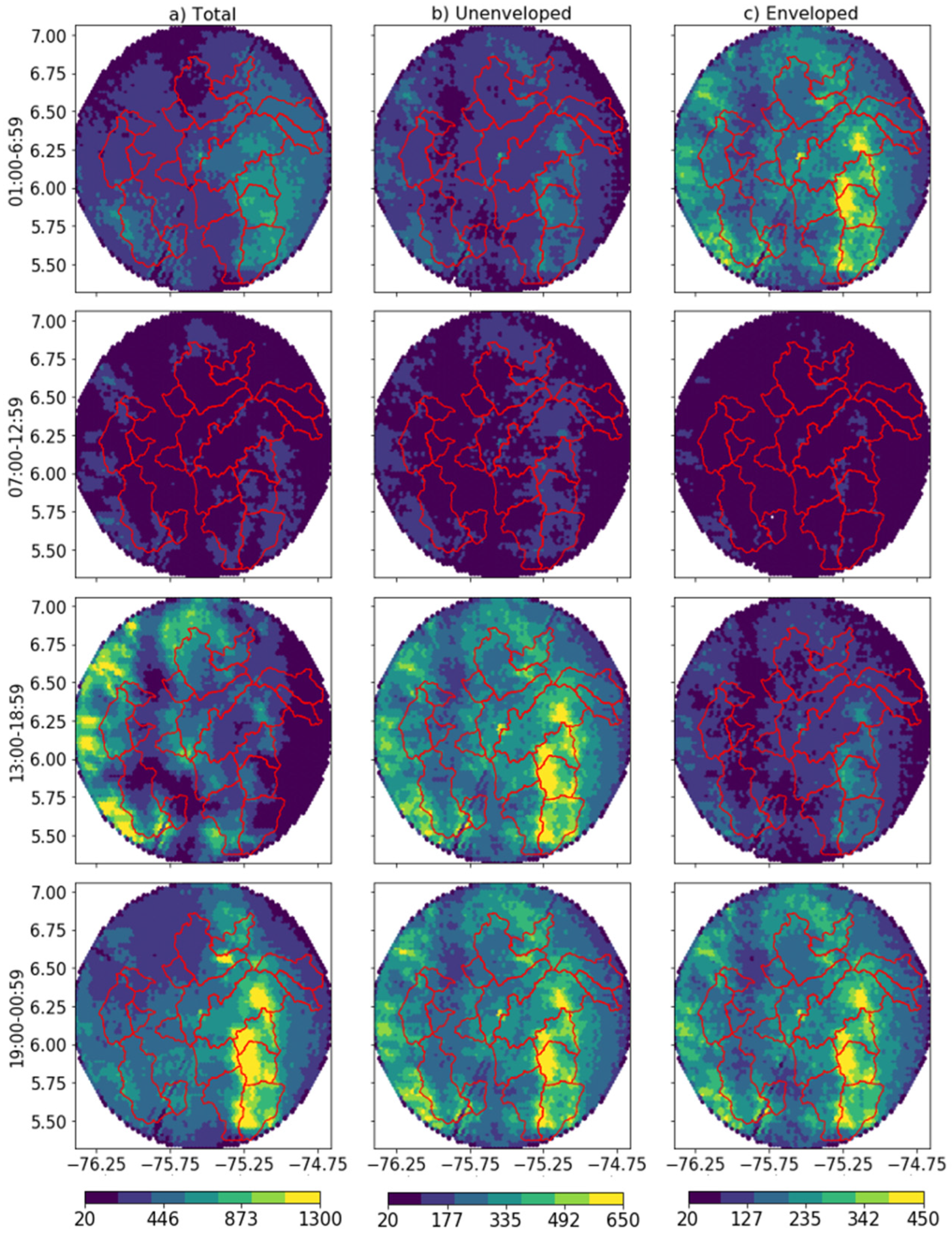
In Figure 7, we closely observe the described temporal evolution of the convective system. In it, we colored the spatial domain using the total count of systems falling in pixels of 1 . Considering the significant count differences, we used different ranges to color each column of the figure. Moreover, we divided the results using a time step of six hours starting at 1:00 A.M. Since the total count of cases for the columns was significantly different, we kept independent color bars for each.
Column a in Figure 7 presents the spatiotemporal results of all the convective systems and expands the description presented in Figure 6. According to Figure 7, the morning hours have some convective activity (1st row). This activity reaches its minimum values between 7 A.M. and noon (2nd row). Then, during the afternoon, convective systems occur over the West and center regions of the domain (3rd row). Finally, during the night, the storms occur over the East (4th row).
Columns b and c in Figure describe the results for the unenveloped and enveloped system cases. Unenveloped systems (column b) exhibit a predominant formation over the eastern region between the afternoon and midnight (third and fourth rows). Moreover, they decrease during the morning (first row) and mostly disappear during the day (second row). Enveloped systems dominate the East, with some occurrences over the West.
Moreover, the lag described in Figure 6 between the enveloped and unenveloped systems is also present. During the afternoon, unenveloped systems intensify while some envelopes occur (third row). During the night (fourth row), both categories increase. Then, in the morning, enveloped systems become dominant. According to our results, enveloped and unenveloped systems categories’ temporal distributions coincide with the described evolution of the convective system [40]. Moreover, their occurrence coincides with the region’s descriptions of orographic rainfall formation [53,54].
According to Figure 7, the convective systems have well-defined spatiotemporal distributions. Most convective systems occurred in the East between noon and midnight. Their occurrence coincided with reported flash floods and shallow landslide events [13,14]. They also coincided with descriptions of the Colombian Andean climatology [54,55]. The results presented here are likely intertwined with several climatological variables. However, exploring that connection is out of our scope. Future work may explore that link and how to use the results presented in the vulnerability analysis and risk assessment.
Figure 8 summarizes the spatial distribution regardless of the daytime. According to Figure 8a, most convective systems occur in the East, specifically in Rio Playas, Rio Calderas, and Rio Verde (see Figure 1). There are also minor convective accumulations in the West near Rio Penderisco and Rio San Juan watersheds, and in the north near the outlet of Rio Grande. Unenveloped systems follow a similar localization (Figure 8b), with a significant occurrence increase near the boundaries of the watersheds. On the other hand, enveloped systems are more sparse over the region, being dominant in the West and in the East in the watersheds of Rio Verde and Samana.
The localization of the convective systems coincides with the region’s topography. Unenveloped systems mainly occur over the watersheds’ boundary lines, usually the steepest areas. Moreover, they occur more often in watersheds with a significant elevation difference, in this case, the Rio Caldera, Rio Verde, and Samana watersheds with elevation gradients of around 2000 . On the other hand, enveloped systems behave like a remanent of unenveloped ones being distributed downstream of the described regions.
The given description is of significant value, and the localization of the unenveloped systems can help determine vulnerable regions.
4.3. Connections with the Topography
According to our results, several convective systems tend to occur near the divisor lines of watersheds with high elevation gradients (see Figure 9a,b). However, some watersheds had a high elevation gradient, but the count of convective systems was low. In this section, we explored further the connection between the convective systems’ occurrence and the characteristics of the watersheds. Here, we compared the localization of the convective systems with the area, aspect, and elevation gradient of the region’s watersheds.
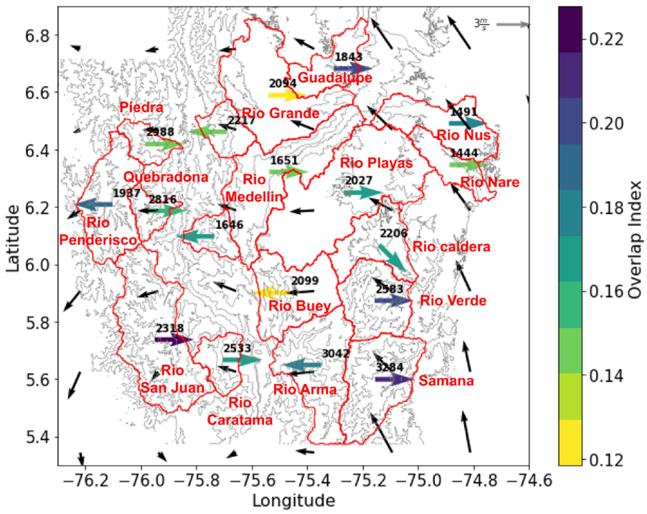
Figure 10 presents the 18 watersheds, their aspects, the topography, and the prevailing direction of the wind at 750 (around 2500 m above sea level). Moreover, in the figure, we colored the aspects of the watersheds with the overlapping index, . The index measures the area shared between a convective system and a watershed. In our case, oscillated between 0.12 and 0.22.
According to Figure 10, the Samana, Rio Verde, Guadalupe (East), and Rio San Juan (West) watersheds have the highest values. In the four cases, the aspect is opposite to the wind, and the elevation difference is above 2000 , except for Guadalupe where it is 1843 . Nevertheless, this analysis has been conducted using the preferential wind direction, and, in many cases, the results presented here (3) may not be fulfilled. Moreover, it seems that additional features are involved, since some watersheds exhibit similar topographical features, but lower values.
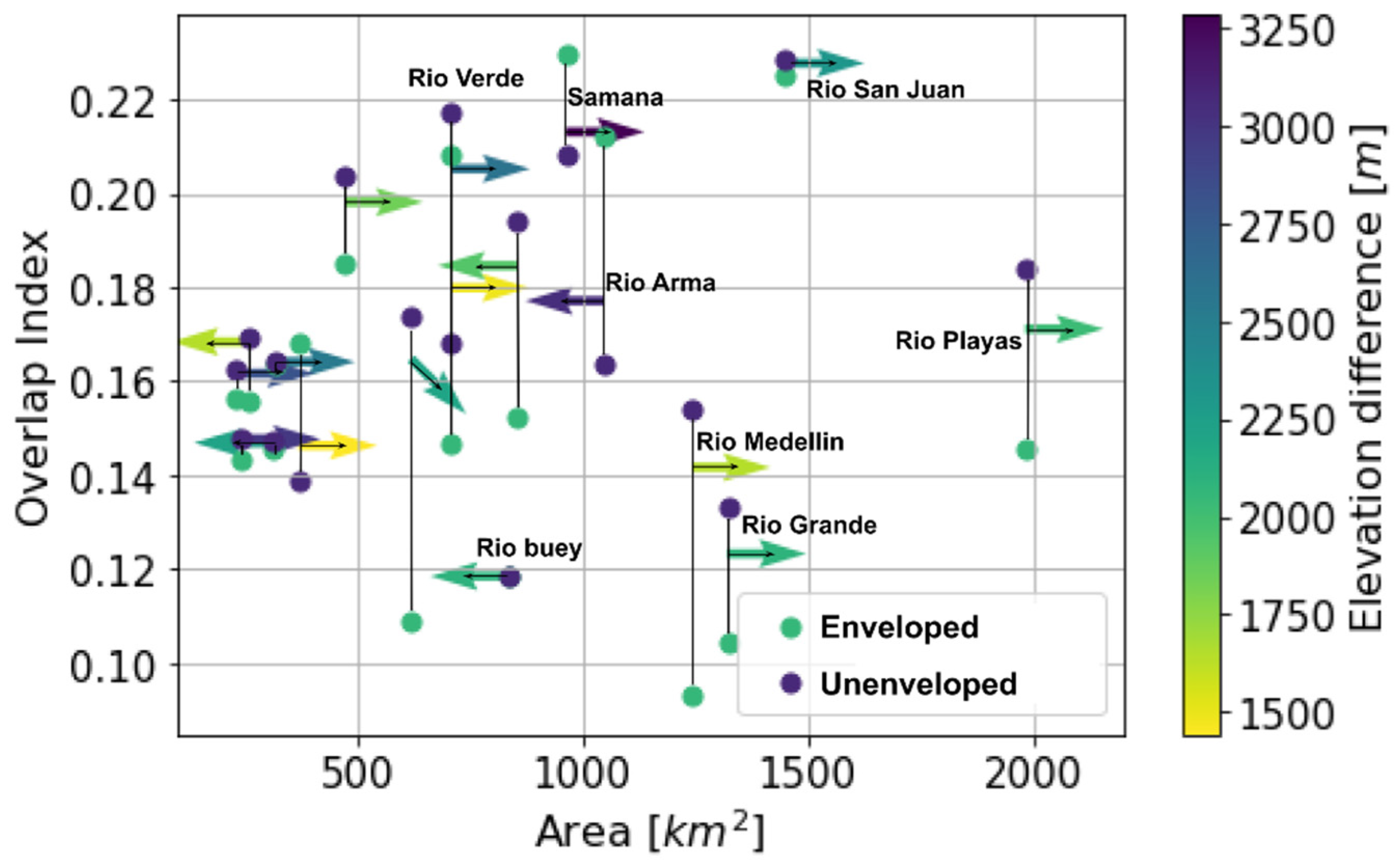
Additionally, we compared with the upstream area, aspect, and elevation gradient of the watersheds (Figure 11). In the figure, the position of the arrow coincides with the area and the overlap index, , computed for each watershed. The direction represents the aspect, and the color the elevation gradient. Moreover, the circles represent the index for the enveloped (green) and unenveloped (purple) systems.
According to Figure 11, the unenveloped and enveloped values change among watersheds. In thirteen out of the eighteen watersheds, unenveloped is dominant. Moreover, enveloped is foremost in watersheds with upstream areas of around 1000 or less. The difference between the enveloped and unenveloped decreases towards 0.16 for watersheds with areas around 500 . On the other hand, with some exceptions, watersheds with high elevation differences tend to exhibit high values, a condition also influenced by their aspect. Watersheds, such as Samana, Rio Verde, and Rio San Juan, have a high , areas greater than 500 , and elevation differences above 2,000. The given description presents more information regarding the required local conditions for the occurrence of convective systems. However, the analyzed watersheds are large compared to the mean area of the convective systems (24 , see Table 1). Therefore, we expanded our analysis using the boundary sub-watersheds of orders 3, 4, and 5.
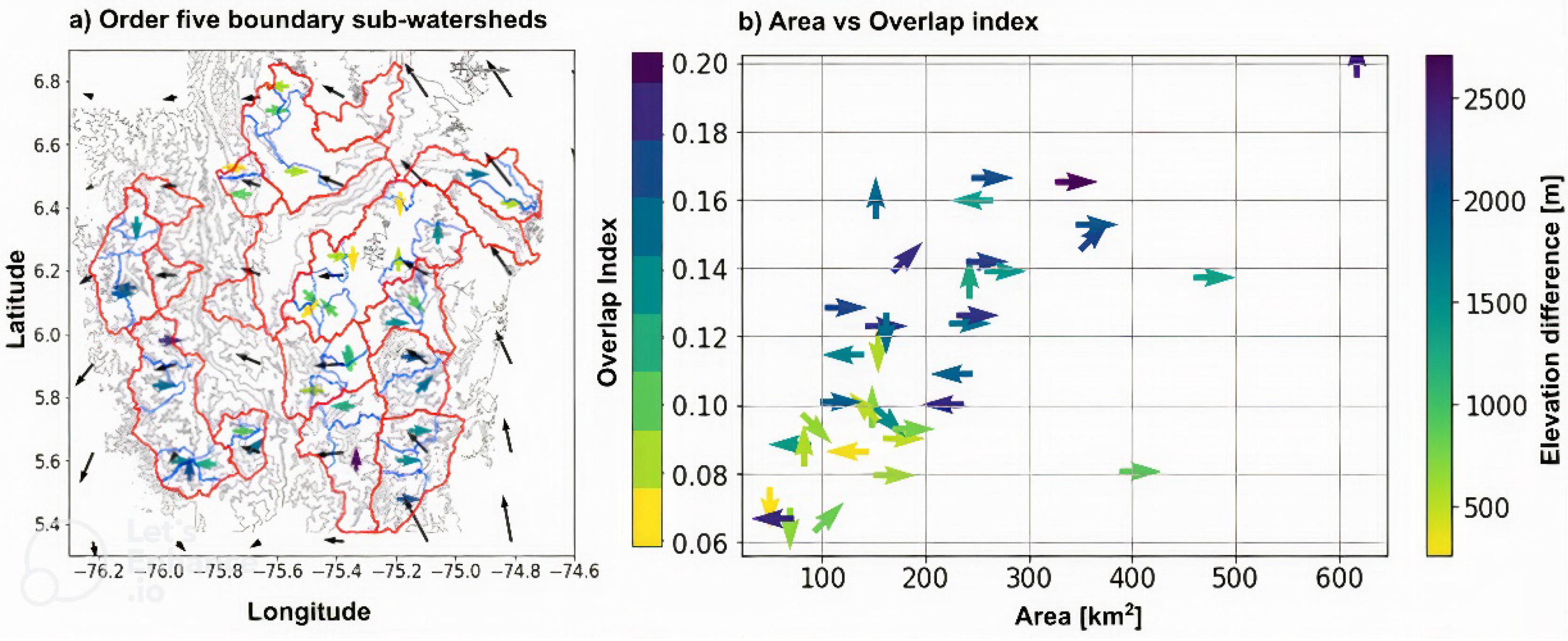
The boundary sub-watersheds had no upstream tributaries and, in most cases, shared the divisor line with its containing watershed. We used boundary sub-watersheds of orders 3, 4, and 5. In the case of order 5, we obtained between two and three sub-watersheds per watershed (blue borders in Figure 12a). Moreover, each sub-watershed had its preferential aspect. According to Figure 12a, watersheds with an aspect opposite to the wind direction tended to have a larger . In addition, the relationship between the upstream area, elevation difference, and became more evident (Figure 12b). Larger areas usually had increased elevation gradients and values.
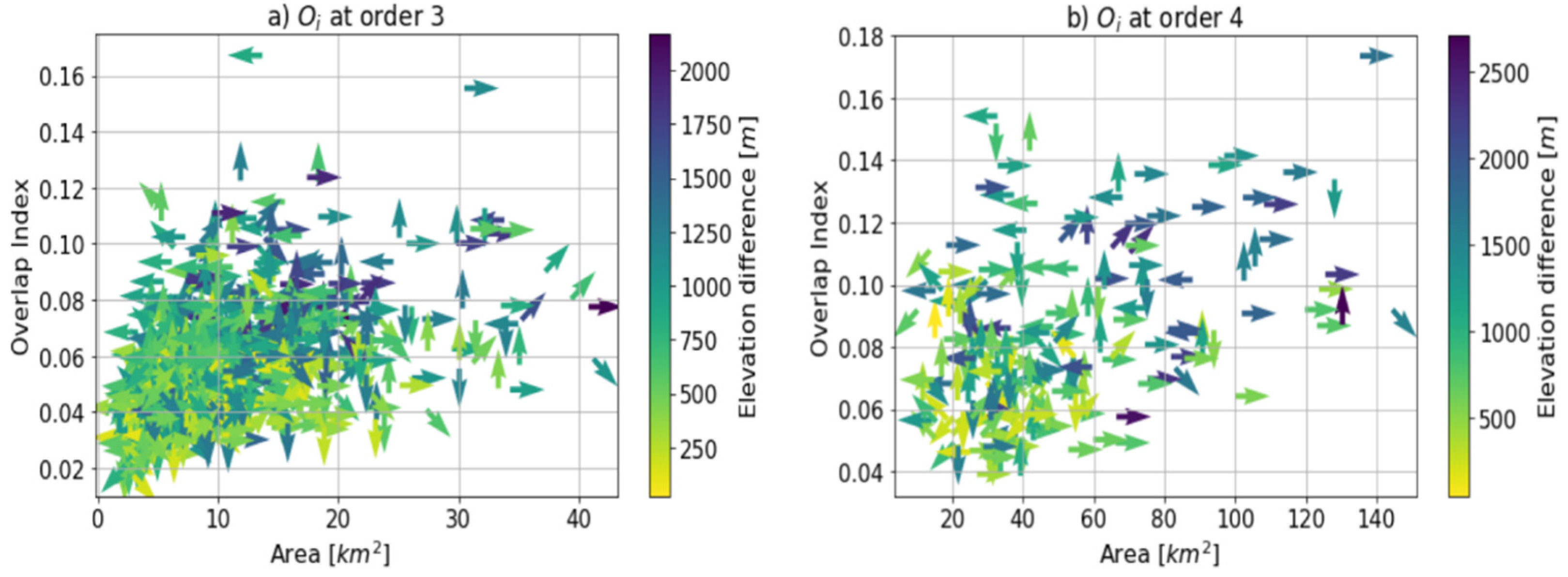
Boundary sub-watersheds of orders 3 and 4 (Figure 13a,b) had a pattern where the overlap index increased with the area and the elevation difference. However, this trend had noise. In order 3 sub-watersheds (Figure 13a), areas between 10 and 40 had similar maximum values. Nevertheless, most of the cases with a high index were sub-watersheds facing East with elevation differences above 1500 . In the case of order 4 sub-watersheds (Figure 13b), there was an increase in the values and the trend with the area was evident. Moreover, the aspect and the elevation difference keep playing a significant role.
The occurrence of convective systems was linked to the elevation difference and aspect of the watersheds at several scales. We analyzed this relationship by defining an overlap index between watersheds and the identified convective systems. According to our results, watersheds with a high elevation gradient and an aspect opposite to the mean wind direction are more likely to develop deep convective systems. Nevertheless, further work is required to establish a link with the topography.
5. Conclusions
This work assessed the convective systems observed in the Colombian Andean region using local meteorological radar data between 2014 and 2017. Furthermore, we expanded our identification by defining two categories: enveloped and unenveloped convective systems. In addition, we compared the area, reflectivity, and localization of the systems. Finally, we proposed a novel method to explore possible interactions between the region’s topography and the occurrence of convective systems. In the topography interaction analysis, we used 18 watersheds and their boundary sub-watersheds of orders 3, 4, and 5. We identified some features of the convective storms of the region along with the areas and times where they usually occurred.
The characteristics of the deep convective systems depended on the stage of their evolution and the mechanisms behind them. A convective storm usually starts as an individual or as a collection of small systems that form a deep system and finally evolves into a stratiform formation with small convective systems [56]. The proper identification of the described evolution requires a tracking algorithm, such as TITAN [57]. Moreover, additional identification algorithms may present more insights into their properties [58]. However, implementing such algorithms in the region is beyond the work presented here. Instead, we introduced a classification of enveloped and unenveloped convective systems.
We described the differences between the region’s deep convective (unenveloped) and clustered (enveloped) systems. Unenveloped systems exhibited higher reflectivity, larger areas, and a higher connection with the topography. On the other hand, enveloped systems behave similar to a late stage of deep convection. This conclusion is also supported by the occurrence time of both types of systems. While unenveloped ones developed between the afternoon and midnight, enveloped systems occurred during the night and morning. The described oscillations may be linked to the energy and humidity availability during the day and the eventual cooling during the night. Nevertheless, more work is required in this direction to develop a more robust conclusion. Furthermore, our approach is a step forward in understanding the mechanisms behind the occurrence of intense storms in the region.
Our analysis also found that deep convective storms occur more often over topographies with specific characteristics. The elevation gradient of the terrain and its aspect relative to the local wind direction were two critical features. We explored the relationship with the topography by analyzing the overlap between the convective systems, the ERA-5 wind at 750 and hundreds of watersheds. According to our results, convective systems occur more often in areas with high topographical gradients, where the aspect is opposite to the wind direction. This result coincides with other studies performed in the region around rainfall and topography [55,59]. Moreover, similar results linking topography and convective rainfall have been reported in other regions [60,61,62,63,64]. However, our analysis does not fully describe the convective storms’ spatial distributions. Future work may include additional meteorological variables and use different ways to assess the connection with topography.
Our results are significant for the hydrologic community and the region’s stakeholders. The characterization presented here identified the areas prone to deep convective storms. Furthermore, joint with landscape information, it could help identify areas in which flash floods and landslides may occur. Moreover, the analysis presented here could be easily replicated and improved, helping to identify vulnerable areas in other regions.
Funding
This work was completed with support from the Iowa Flood Center and SIATA. MID-America Transportation Center (Grant number: 69A3551747107).
Informed Consent Statement
Not applicable.
Data Availability Statement
The data that support the findings of this study are available from the corresponding author upon reasonable request.
Acknowledgments
The authors wish to thank the Sistema de Alertas Tempranas Ambientales (SIATA).
Conflicts of Interest
The authors declare no conflict of interest.
References
- Agyakwah, W.; Lin, Y.-L. Generation and enhancement mechanisms for extreme orographic rainfall associated with Typhoon Morakot (2009) over the Central Mountain Range of Taiwan. Atmospheric Res. 2020, 247, 105160. [Google Scholar] [CrossRef]
- Anders, A.M.; Roe, G.H.; Hallet, B.; Montgomery, D.R.; Finnegan, N.J.; Putkonen, J. Spatial Patterns of Precipitation and Topography in the Himalaya. Geol. Soc. Am. 2006, 2398, 39–53. [Google Scholar]
- Barrett, B.S.; Garreaud, R.; Falvey, M. Effect of the Andes Cordillera on Precipitation from a Midlatitude Cold Front. Mon. WeatherRev. 2009, 137, 3092–3109. [Google Scholar] [CrossRef] [Green Version]
- Barros, A.P.; Kim, G.; Frajka-Williams, E.; Nesbitt, S. Probing Orographic Controls in the Himalayas during the Monsoon Using Satellite Imagery. Nat. Hazards Earth Syst. Sci. 2004, 4, 29–51. [Google Scholar] [CrossRef] [Green Version]
- Barros, A.P.; Joshi, M.; Putkonen, J.; Burbank, D.W. A Study of the 1999 Monsoon Rainfall in a Mountainous Region in Central Nepal Using TRMM Products and Rain Gauge Observations. Geophys. Res. Lett. 2000, 15, 3683–3686. [Google Scholar] [CrossRef]
- Barros, A.P.; Lang, T.J. Monitoring the Monsoon in the Himalayas: Observations in Central Nepal, June 2001. Mon. Weather Rev. 2003, 131, 1408–1427. [Google Scholar] [CrossRef]
- Bedoya-Soto, J.M.; Aristizábal, E.; Carmona, A.M.; Poveda, G. Seasonal Shift of the Diurnal Cycle of Rainfall Over Medellin’s Valley, Central Andes of Colombia (1998–2005). Front. Earth Sci. 2019, 7, 92. [Google Scholar] [CrossRef]
- Bowman, K.P.; Fowler, M.D. The Diurnal Cycle of Precipitation in Tropical Cyclones. J. Clim. 2015, 28, 5325–5334. [Google Scholar] [CrossRef]
- Braud, I.; Ayral, P.-A.; Bouvier, C.; Branger, F.; Delrieu, G.; Le Coz, J.; Nord, G.; Vandervaere, J.-P.; Anquetin, S.; Adamovic, M.; et al. Multi-Scale Hydrometeorological Observation and Modelling for Flash Flood Understanding. Hydrol. Earth Syst. Sci. 2014, 18, 3733–3761. [Google Scholar] [CrossRef] [Green Version]
- Camarasa-Belmonte, A.M. Flash Floods in Mediterranean Ephemeral Streams in Valencia Region (Spain). J. Hydrol. 2016, 541, 99–115. [Google Scholar] [CrossRef]
- Dixon, M.; Wiener, G. TITAN: Thunderstorm Identification, Tracking, Analysis, and Nowcasting-A Radar-Based Methodology. J. Atmos. Ocean. Technol. 1993, 10, 785–797. [Google Scholar] [CrossRef]
- Doswell, C.A.; Harold, E.B.; Robert, A.M. Flash Flood Forecasting: An Ingredients-Based Methodology. Weather Forecast. 1996, 11, 560–581. [Google Scholar] [CrossRef]
- Dowell, D.C. Severe Convective Storms; American Meteorological Society: Boston, MA, USA, 2001. [Google Scholar]
- Ehlschlaeger, C. Using the AT Search Algorithm to Develop Hydrologic Models from Digital Elevation Data. In Proceedings of the International Geographic Information Systems (IGIS) Symposium’89, Baltimore, MD, USA, March 1989; Volume 56, pp. 275–281. [Google Scholar]
- Froidevaux, P.; Martius, O. Exceptional integrated vapour transport toward orography: An important precursor to severe floods in Switzerland. Q. J. R. Meteorol. Soc. 2016, 142, 1997–2012. [Google Scholar] [CrossRef] [Green Version]
- Futyan, J.M.; Del Genio, A.D. Deep Convective System Evolution over Africa and the Tropical Atlantic. J. Clim. 2007, 20, 5041–5060. [Google Scholar] [CrossRef]
- Garreaud, R.; Rutllant, J. Coastal Lows in North-Central Chile: Numerical Simulation of a Typical Case. Mon. Weather Rev. 2003, 131, 891–908. [Google Scholar] [CrossRef]
- Garreaud, R.; Fuenzalida, H.A. The Influence of the Andes on Cutoff Lows: A Modeling Study*. Mon. Weather Rev. 2007, 135, 1596–1613. [Google Scholar] [CrossRef] [Green Version]
- Garrote, J.; Alvarenga, F.; Diez-Herrero, A. Quantification of Flash Flood Economic Risk Using Ultra-Detailed Stage–Damage Functions and 2-D Hydraulic Models. J. Hydrol. 2016, 541, 611–625. [Google Scholar] [CrossRef]
- Gultepe, I. 56 Advances in Geophysics. In Mountain Weather Observation and Modeling; Elsevier Ltd.: Amsterdam, The Netherlands, 2015. [Google Scholar] [CrossRef]
- Hilgendorf, E.R.; Johnson, R.H. A Study of the Evolution of Mesoscale Convective Systems Using WSR-88D Data. Weather Forecast. 1998, 13, 437–452. [Google Scholar] [CrossRef]
- Houze, R.A., Jr. Mesoscale Convective Systems. Rev. Geophys. 2004, 42, 1–43. [Google Scholar] [CrossRef] [Green Version]
- Houze, R.A. Orographic Control of Precipitation: What Are We Learning from MAP. MAP Newsl. 2001, 14, 3–5. [Google Scholar]
- Orographic Effects on Precipitating Clouds. Rev. Geophys. 2012, 50, 1–47.
- Houze, R.A., Jr.; Rasmussen, K.L.; Zuluaga, M.D.; Brodzik, S.R. The variable nature of convection in the tropics and subtropics: A legacy of 16 years of the Tropical Rainfall Measuring Mission satellite. Rev. Geophys. 2015, 53, 994–1021. [Google Scholar] [CrossRef] [PubMed]
- Hoyos, C.D.; Ceballos, L.I.; Pérez-Carrasquilla, J.S.; Sepúlveda, J.; López-Zapata, S.M.; Zuluaga, M.D.; Velásquez, N.; Herrera-Mejía, L.; Hernández, O.; Guzmán-Echavarría, G.; et al. Meteorological conditions leading to the 2015 Salgar flash flood: Lessons for vulnerable regions in tropical complex terrain. Nat. Hazards Earth Syst. Sci. 2019, 19, 2635–2665. [Google Scholar] [CrossRef] [Green Version]
- Jaramillo, L.; Poveda, G.; Mejía, J.F. Mesoscale Convective Systems and Other Precipitation Features over the Tropical Americas and Surrounding Seas as Seen by TRMM. Int. J. Climatol. 2017, 37, 380–397. [Google Scholar] [CrossRef]
- Kingsmill, D.E.; Persson, P.O.G.; Haimov, S.; Shupe, M.D. Mountain Waves and Orographic Precipitation in a Northern Colorado Winter Storm. Q. J. R. Meteorol. Soc. 2015, 142, 836–853. [Google Scholar] [CrossRef]
- Li, Y.; Zhang, G.; Doviak, R.J.; Lei, L.; Cao, Q. A New Approach to Detect Ground Clutter Mixed with WeatherSignals. IEEE Trans. Geosci. Remote Sens. 2012, 51, 2373–2387. [Google Scholar] [CrossRef]
- Lilly, D.K. A Severe Downslope Windstorm and Aircraft Turbulence Event Induced by a Mountain Wave. J. Atmos. Sci. 1978, 35, 59–77. [Google Scholar] [CrossRef] [Green Version]
- Lin, Y.-L.; Chiao, S.; Wang, T.-A.; Kaplan, M.L.; Weglarz, R.P. Some Common Ingredients for Heavy Orographic Rainfall. Weather Forecast. 2001, 16, 633–660. [Google Scholar] [CrossRef]
- Llasat, M.C.; Marcos, R.; Turco, M.; Gilabert, J.; Llasat-Botija, M. Trends in Flash Flood Events versus Convective Precipitation in the Mediterranean Region: The Case of Catalonia. J. Hydrol. 2016, 541, 24–37. [Google Scholar] [CrossRef] [Green Version]
- Maddox, R.A.; Hoxit, L.R.; Chappell, C.F.; Caracena, F. Comparison of Meteorological Aspects of the Big Thompson and Rapid City Flash Floods. Mon. Weather Rev. 1978, 106, 375–389. [Google Scholar] [CrossRef] [Green Version]
- Mohr, K.I.; Slayback, D.; Yager, K. Characteristics of Precipitation Features and Annual Rainfall during the TRMM Era in the Central Andes. J. Clim. 2014, 27, 3982–4001. [Google Scholar] [CrossRef] [Green Version]
- Posada-Marín, J.A.; Rendón, A.M.; Salazar, J.F.; Mejía, J.F.; Villegas, J.C. WRF Downscaling Improves ERA-Interim Representation of Precipitation around a Tropical Andean Valley during El Niño: Implications for GCM-Scale Simulation of Precipitation over Complex Terrain. Clim. Dyn. 2019, 52, 3609–3629. [Google Scholar] [CrossRef]
- Poveda, G.; Jaramillo, A.; Gil, M.M.; Quiceno, N.; Mantilla, R. Seasonally in ENSO-Related Precipitation, River Discharges, Soil Moisture, and Vegetation Index in Colombia. Water Resour. Res. 2001, 37, 2169–2178. [Google Scholar] [CrossRef]
- Poveda, G.; Alvaro, J.; Marta, M.G.; Natalia, Q.; Ricardo, M. Water Resources Research—2001—Poveda—Seasonally in ENSO-related Precipitation River Discharges Soil Moisture and.Pdf. Water Resour. Reseach 2001, 37, 20169–20178. [Google Scholar]
- Germán, P.; Oscar, M.; Paula, A.; Juan, Á.; Paola, A.; Hernán, M.; Luis, S.; Vladimir, T.; Sara, V. Influencia Del ENSO, Oscilación Madden-Julian, Ondas Del Este, Huracanes y Fases de La Luna En El Ciclo Diurno de Precipitación En Los Andes Tropicales de Colombia. Meteorol. Colomb. 2002, 5, 3–12. [Google Scholar]
- La Hidroclimatología De Colombia: Una Síntesis Desde La Escala Inter-Decadal Hasta La Escala Diurna. Rev. De La Acad. Colomb. De Cienc. 2004, XXVIII, 201–222.
- Purnell, D.J.; Kirshbaum, D.J. Synoptic Control over Orographic Precipitation Distributions during the Olympics Mountains Experiment (OLYMPEX). Mon. Weather Rev. 2018, 146, 1023–1044. [Google Scholar] [CrossRef]
- Rasmussen, K.L.; Chaplin, M.M.; Zuluaga, M.; Houze, R.A., Jr. Contribution of Extreme Convective Storms to Rainfall in South America. J. Hydrometeorol. 2015, 17, 353–367. [Google Scholar] [CrossRef]
- Rasmussen, K.L.; Houze, R.A. Convective Initiation near the Andes in Subtropical South America. Mon. Weather Rev. 2016, 144, 2351–2374. [Google Scholar] [CrossRef]
- Rasmussen, K.L.; Robert, A.H. A Flash-Flooding Storm at the Steep Edge of High Terrain. Bull. Am. Meteorol. Soc. 2012, 93, 1713–1724. [Google Scholar] [CrossRef] [Green Version]
- Rasmussen, K.L.; Zuluaga, M.D.; Houze, R.A., Jr. Severe Convection and Lightning in Subtropical South America. Geophys. Res. Lett. 2014, 41, 7359–7366. [Google Scholar] [CrossRef]
- Roe, G.H. Orographic Precipitation. Annu. Rev. Earth Planet. Sci. 2005, 33, 645–671. [Google Scholar] [CrossRef]
- Romatschke, U.; Houze, R.A. Characteristics of Precipitating Convective Systems in the South Asian Monsoon. J. Hydrometeorol. 2001, 12, 3–26. [Google Scholar] [CrossRef]
- Romatschke, U.; Medina, S.; Houze, R.A. Regional, Seasonal, and Diurnal Variations of Extreme Convection in the South Asian Region. J. Clim. 2010, 23, 419–439. [Google Scholar] [CrossRef] [Green Version]
- Roy Bhowmik, S.K.; Roy, S.S.; Kundu, P.K. Analysis of Large-Scale Conditions Associated with Convection over the Indian Monson Region. Int. J. Climatol. 2008, 4, 797–821. [Google Scholar] [CrossRef]
- Rozalis, S.; Morin, E.; Yair, Y.; Price, C. Flash Flood Prediction Using an Uncalibrated Hydrological Model and Radar Rainfall Data in a Mediterranean Watershed under Changing Hydrological Conditions. J. Hydrol. 2010, 394, 245–255. [Google Scholar] [CrossRef]
- Ruiz-Villanueva, V.; Borga, M.; Zoccatelli, D.; Marchi, L.; Gaume, E.; Ehret, U. Extreme Flood Response to Short-Duration Convective Rainfall in South-West Germany. Hydrol. Earth Syst. Sci. 2012, 16, 1543–1559. [Google Scholar] [CrossRef] [Green Version]
- Characterisation of Flash Floods in Small Ungauged Mountain Basins of Central Spain Using an Integrated Approach. Catena 2013, 110, 32–43. [CrossRef]
- Schumacher, R.; Johnson, R.H. Organization and Environmental Properties of Extreme-Rain-Producing Mesoscale Convective Systems. Mon. Weather Rev. 2005, 133, 961–976. [Google Scholar] [CrossRef]
- Chumchean, S.; Seed, A.; Sharma, A. An Operational Approach for Classifying Storms in Real-Time Radar Rainfall Estimation. J. Hydrol. 2008, 363, 1–17. [Google Scholar] [CrossRef]
- Smith, R.B.; Barstad, I.; Bonneau, L. Orographic Precipitation and Oregon’s Climate Transition. J. Atmos. Sci. 2005, 62, 177–191. [Google Scholar] [CrossRef]
- Steiner, M.; Houze, R.A.; Yuter, S. Climatological Characterization of Three-Dimensional Storm Structure from Operational Radar and Rain Gauge Data. J. Appl. Meteorol. 1995, 34, 1978–2007. [Google Scholar] [CrossRef]
- Urrea, V.; Andrés, O.; Oscar, M. Seasonality of Rainfall in Colombia. Water Resour. Res. 2019, 55, 4149–4162. [Google Scholar] [CrossRef]
- Valenzuela, R.A.; David, E.K. Terrain-Trapped Airflows and Orographic Rainfall along the Coast of Northern California. Part II: Horizontal and Vertical Structures Observed by a Scanning Doppler Radar. Mon. Weather Rev. 2018, 146, 2381–2402. [Google Scholar] [CrossRef]
- Vargas, G.; Hernández, Y.; Pabón, J.D. La Niña Event 2010–2011: Hydroclimatic Effects and Socioeconomic Impacts in Colombia. In Climate Change, Extreme Events and Disaster Risk Reduction: Towards Sustainable Development Goals; Mal, S., Singh, R.B., Huggel, C., Eds.; Springer International Publishing: Cham, Switerland, 2018; pp. 217–232. [Google Scholar] [CrossRef]
- Velásquez, N.; Hoyos, C.D.; Vélez, J.I.; Zapata, E. Reconstructing the 2015 Salgar Flash Flood Using Radar Retrievals and a Conceptual Modeling Framework in an Ungauged Basin. Hydrol. Earth Syst. Sci. 2020, 24, 1367–1392. [Google Scholar] [CrossRef] [Green Version]
- Vivekanandan, J.; Yates, D.N.; Brandes, E.A. The Influence of Terrain on Rainfall Estimates from Radar Reflectivity and Specific Propagation Phase Observations. J. Atmos. Ocean. Technol. 1999, 16, 837–845. [Google Scholar] [CrossRef]
- Wang, Y.; Tang, L.; Chang, P.-L.; Tang, Y.-S. Separation of Convective and Stratiform Precipitation Using Polarimetric Radar Data with a Support Vector Machine Method. Atmos. Meas. Tech. 2021, 14, 185–197. [Google Scholar] [CrossRef]
- Xie, S.-P.; Xu, H.; Saji, N.H.; Wang, Y.; Liu, W.T. Role of Narrow Mountains in Large-Scale Organization of Asian Monsoon Convection. J. Clim. 2006, 19, 3420–3429. [Google Scholar] [CrossRef]
- Yu, C.-K.; Smull, B.F. Airborne Doppler Observations of a Landfalling Cold Front Upstream of Steep Coastal Orography. Mon. Weather Rev. 2000, 128, 1577–1603. [Google Scholar] [CrossRef]
- Zuluaga, M.; Houze, R.A. Extreme Convection of the Near-Equatorial Americas, Africa, and Adjoining Oceans as Seen by TRMM. Mon. Weather Rev. 2015, 143, 298–316. [Google Scholar] [CrossRef] [Green Version]
Figure 1.
Region of analysis, radar localization is presented at the center of the image, and gray circles correspond to radar radii of 30 and 90 . Yellow to dark blue colors represents the stream network Horton orders from 3 to 6.
Figure 1.
Region of analysis, radar localization is presented at the center of the image, and gray circles correspond to radar radii of 30 and 90 . Yellow to dark blue colors represents the stream network Horton orders from 3 to 6.

Figure 2.
A schematic representation of the proposed methodology to separate enveloped and unenveloped systems. (a) Binaries of convective (
) and stratiform () systems are separated, takes values of 0 and 2, takes values of 0 and 1. (b) is eroded and is obtained, then is obtained by filling holes in the binary. (c) is computed as the sum of and . values equal to 2 correspond to unenveloped convective systems, and values of 3 correspond to enveloped systems.

Figure 3.
Example of a classified radar image. (a) Original reflectivity image in dBZ, (b) identification of convective (yellow) and stratiform systems (purple), (c) ID assignation to each convective system, and (d) identification of enveloped (orange) and unenveloped (green) systems.
Figure 3.
Example of a classified radar image. (a) Original reflectivity image in dBZ, (b) identification of convective (yellow) and stratiform systems (purple), (c) ID assignation to each convective system, and (d) identification of enveloped (orange) and unenveloped (green) systems.

Figure 4.
Example of boundary sub-watersheds definitions (a–c) and overlap index estimations (d). The three top panels describe the boundary sub-watersheds of orders 3, 4, and 5 for the Samana watershed.
Figure 4.
Example of boundary sub-watersheds definitions (a–c) and overlap index estimations (d). The three top panels describe the boundary sub-watersheds of orders 3, 4, and 5 for the Samana watershed.

Figure 5.
Reflectivity and area for 10,000 randomly selected systems. Circles correspond to convective systems, triangles to stratiform systems, and the color is associated with the variability of the reflectivity inside the system. Vertical histograms present the PDF for the mean reflectivity for both types of systems, and the horizontal histograms correspond to the PDF of the area.

Figure 6.
Reflectivity and area comparison for enveloped (triangles) and unenveloped (circles) connective systems. Colors represent the standard deviation. Vertical and horizontal histograms present the PDFs for the reflectivity and areas, respectively.
Figure 6.
Reflectivity and area comparison for enveloped (triangles) and unenveloped (circles) connective systems. Colors represent the standard deviation. Vertical and horizontal histograms present the PDFs for the reflectivity and areas, respectively.

Figure 7.
Hourly distributions of the occurrence of total convective (dashed blue), unenveloped (purple), and enveloped (yellow) systems.
Figure 7.
Hourly distributions of the occurrence of total convective (dashed blue), unenveloped (purple), and enveloped (yellow) systems.

Figure 8.
Two-dimensional histogram of convective centroid localization inside the radar region. Column (a) corresponds to total convective localization, (b) unenveloped systems, and (c) enveloped ones. The colors represent the count of elements. Color bars correspond to each of the columns.
Figure 8.
Two-dimensional histogram of convective centroid localization inside the radar region. Column (a) corresponds to total convective localization, (b) unenveloped systems, and (c) enveloped ones. The colors represent the count of elements. Color bars correspond to each of the columns.

Figure 9.
Two-dimensional histogram of convective centroid localization inside the radar region. (a) Total convective systems. Figures (b,c) correspond to unenveloped and enveloped systems, respectively. The black lines are topographical contour lines representing increments of 1000 .
Figure 9.
Two-dimensional histogram of convective centroid localization inside the radar region. (a) Total convective systems. Figures (b,c) correspond to unenveloped and enveloped systems, respectively. The black lines are topographical contour lines representing increments of 1000 .

Figure 10.
Spatial distribution of the overlap index. The bold arrows represent the aspect of the watersheds, while their color corresponds to the overlap index. Black arrows represent the ERA-5 wind speed and direction. The red and black lines are the watershed boundaries and topography (500 m). The numbers represent the elevation gradient.

Figure 11.
Overlap index in function of the area, aspect, and elevation gradient of the watersheds. The arrows correspond to the analyzed watershed denoting its main aspect. The arrows represent the watershed aspect, and the color corresponds to the elevation gradient (
). The purple and green circles represent the overlap index, , for the enveloped and unenveloped systems.

Figure 12.
Spatial distribution of the overlap index for the boundary sub-watersheds or orders 5. In panel (a), the blue lines represent the sub-watersheds, the colored arrows the aspect (direction) and the overlap index (color), and the black arrows represent the ERA-5 wind at 750 . In panel (b), the arrows represent the aspect, and their color is the elevation difference.

Figure 13.
Overlap index for boundary sub-watersheds of orders 3 (a) and 4 (b). The arrows represent the aspect and colors the elevation difference.
Figure 13.
Overlap index for boundary sub-watersheds of orders 3 (a) and 4 (b). The arrows represent the aspect and colors the elevation difference.


Table 1.
Summary values of the systems identified.
| Feature | Stratiform | Convective | Unenveloped | Enveloped |
|---|---|---|---|---|
| ] | 43,000 | 14,000 | 14,000 | 13,200 |
| ] | 47 | 24 | 30 | 15 |
| ] | 445 | 160 | 180 | 131 |
| ] | 1.50 | 1.43 | 1.52 | 1.34 |
| ] | 60 | 33 | 43 | 16 |
| ] | 40 | 60 | 60 | 46 |
| ] | 0.26 | 22 | 22 | 22 |
| ] | 16 | 30 | 32 | 28 |
| ] | 6.6 | 3.7 | 4.1 | 1.6 |
| ] | 10 | 27 | 27 | 27 |
| ] | 27 | 36 | 38 | 30 |
Publisher’s Note: MDPI stays neutral with regard to jurisdictional claims in published maps and institutional affiliations. |
© 2022 by the author. Licensee MDPI, Basel, Switzerland. This article is an open access article distributed under the terms and conditions of the Creative Commons Attribution (CC BY) license (https://creativecommons.org/licenses/by/4.0/).
Share and Cite
MDPI and ACS Style
Velásquez, N. Assessment of Deep Convective Systems in the Colombian Andean Region. Hydrology 2022, 9, 119. https://0-doi-org.brum.beds.ac.uk/10.3390/hydrology9070119
AMA Style
Velásquez N. Assessment of Deep Convective Systems in the Colombian Andean Region. Hydrology. 2022; 9(7):119. https://0-doi-org.brum.beds.ac.uk/10.3390/hydrology9070119
Chicago/Turabian StyleVelásquez, Nicolás. 2022. "Assessment of Deep Convective Systems in the Colombian Andean Region" Hydrology 9, no. 7: 119. https://0-doi-org.brum.beds.ac.uk/10.3390/hydrology9070119
Note that from the first issue of 2016, this journal uses article numbers instead of page numbers. See further details here.