Structural Changes in the Consumption of Beer, Wine and Spirits in OECD Countries from 1961 to 2014

Department of Economics and Business Economics and The Tuborg Centre for Globalisation and Firm Dynamics, Aarhus University, 8210 Aarhus, Denmark
*
Author to whom correspondence should be addressed.
Beverages 2018, 4(1), 8; https://0-doi-org.brum.beds.ac.uk/10.3390/beverages4010008
Submission received: 18 September 2017
/
Revised: 11 December 2017
/
Accepted: 4 January 2018
/
Published: 22 January 2018
(This article belongs to the Special Issue Alcoholic Beverages Market)
Abstract
:Alcohol consumption is usually measured as the simple sum of the per capita consumption of beer, wine and spirits in alcohol equivalents, i.e., assuming the specific beverages to be perfect substitutes. Alternatively, total alcohol consumption can be represented by a vector in the three-dimensional space of beer, wine and spirits, and the concept of angular separation is used to give a structural measurement of the beverage composition. Applying such a methodology, the aim of this paper is to analyse and explain structural changes in alcohol consumption among 21 OECD countries over the period from 1961 to 2014. Overall, the analyses suggest that convergence has taken place in the structural composition of alcohol consumption in the OECD countries. Income, the alcohol consumption level, trade openness and demographic factors are found to be drivers of this development during the last decades.
1. Introduction
Changes in the drinking patterns of wine, beer and spirits have traditionally been of interest in the studies of alcohol and consumer behaviour. Economists have normally analysed the topic in classical consumer theory models, where partial demand functions for beer, wine and spirits have been derived and estimated [1,2,3]. In line with consumer theory, the majority of the empirical studies suggest that own prices, prices of substitutes and income play significant roles for the demand of the various alcohol beverages. However, only a few studies take the mutual interdependence in the demand for the respective beverages into account, and they ignore, for example, the overall demand restrictions in the empirical models [3,4], which complicates the use of the empirical results for analysis of alcohol consumption, structure and convergence in the longer run. From a theoretical point of view, estimating a system of demand equations for the respective beverages would be the best approach, also when investigating the process of convergence. In a modelling framework such as the AIDS model in Deaton and Muellbauer [5], consumption expenditures and prices are included, thus not only capturing price effects but also fulfilling the consistency of household expenditure from the aggregate expenditure restrictions. A similar approach cannot be applied in relation to the convergence topic due to lack of data, where especially valid information on beverage prices are not available. Therefore, more direct methodologies have been used where overall consistency is often fulfilled in a more simplified form [6,7,8,9]. It is found that former differences in the level of per capita intake of beer, wine and spirits among the majority of OECD countries have diminished. Still, studies of convergence may be criticized for not offering much explanation. Furthermore, a critical characteristic in the convergence studies is that the level of consumption is usually measured as the simple sum of the per capita consumption of beer, wine and spirits (measured in alcohol equivalents). Thus, the total alcohol consumption adds the specific beverages as if they were perfect substitutes, which of course is a restrictive assumption.
The aim of this paper is to analyse and explain structural changes using a holistic methodology, developed by Jaffe [10] and Andersen [11], where an alternative point of departure for a study of convergence is suggested. Total alcohol consumption can be represented by a vector including the three elements—beer, wine and spirits—where the length of this vector in a Euclidian space is interpreted as a measure of total alcohol consumption. When assessing or evaluating the structural component in alcohol consumption, the angle between this vector and a vector of unit values is an obvious alternative to traditional measures. From this methodology, the total consumption of alcohol can be decomposed into a component representing the length of the beverage vector and a structural component of beer, wine and spirits which has a value between zero and unity. In the empirical part of the paper, we test this model of structural changes on the data for 21 OECD countries covering the period from 1961 to 2014. The results suggest that ‘between’ as well as ‘within’ differences in the consumption patterns among the included countries have declined. Separating the countries into beer, wine or spirits-drinking countries only reinforces the evidence of diminishing structural differences. The second part of the paper focuses on some explanatory factors for convergence in the consumption patterns, such as income, per capita alcohol consumption, trade openness and demographics, which are formally tested with fixed effects models of the panel data for the OECD countries from 1961 to 2014.
2. Literature Review
Analyses of factors determining the structure of alcohol consumption are often based on a classification, such as beer, wine and spirits countries; cf. this issue appearing in [1,7,8,9,12]. Arguments for this classification are related to climate conditions, religion, regulation in form of taxes and other conditions such as, e.g., openness to trade and globalization, and naturally the historical background and traditions behind the drinking patterns. In the case of beer, Colen and Swinnen state that there is an inverted U-shape relationship between income and beer consumption, and find that openness to trade in beer-drinking countries will diminish the beer share in total alcohol consumption [1,12]. Apart from the overall level of alcohol consumption in a given country, composition with respect to age groups, gender etc. is also of importance when considering the structural consumption development. Deveaux and Sassi use data for twenty OECD countries and find a stability in the overall alcohol consumption levels [13], but, for example, young adults show increasing higher-risk drinking behaviour, and such factors will in the longer run have influence on the structural composition of alcohol consumption. For Russia, a study by Kossova et al. also finds specific internal factors to be of importance for the structure of alcohol consumption, where e.g., unemployment is, somewhat surprisingly, negatively related to the consumption of vodka and beer, but in some years positively related to wine consumption [14].
From these references, it can be concluded that, in terms of the wine, beer and spirits shares, convergence in drinking patterns has to a large degree taken place, although with regional differences as revealed by using a consumption similarity index as done by [9]. However, the empirical evidence is sparse on which factors influence the structural composition of alcohol consumption—an issue to be further investigated in the following parts and a topic that is also put forward in other studies, op. cit. Some studies focus on regularities between the countries [4], who estimates income and price elasticities for eight OECD countries and finds similar levels of the respective elasticities as well as other similarities present in alcohol consumption patterns. The consumption of beer, wine and spirits in ten OECD countries is analysed in [3] and find inelastic demand for all the three kinds of beverages, where beer and wine have income elasticities below unity, and spirits as a luxury good having an above-unity income elasticity. When similar levels of elasticities are present among the OECD countries, we will only expect structural changes if the developments in incomes and prices differ among the countries considered. Likewise, Lee finds a link between alcohol consumption and income using panel data for twenty-seven OECD countries, where differences in alcohol consumption have a causal relationship with either income or health differentials [15]. Alcohol advertising bans may also be assumed to have influence on both the overall level as well as the beverage composition of alcohol consumption, and the OECD countries differ in respect to advertising, with some Nordic countries having restrictive policies, for example. Nelson has tested this topic using a panel data set for seventeen OECD countries and cannot reject a hypothesis of no effect from bans on alcohol consumption [16].
3. The Empirical Model
The methodology1 to be used in the empirical part of the paper can be described as follows. The total alcohol consumption is usually measured as the simple sum of beer, wine and spirits calculated in per capita pure alcohol equivalents:
Naturally, this aggregation assumes full substitutability among the beverages, i.e., the structure of the respective beverages does not matter because the quantities of beer, wine and spirits are just added as stated in (1). In order to address this problem, total alcohol consumption can alternatively be measured by the length of the vector (B, W, S), again defined from the quantities of these beverages. Consequently, the overall level of alcohol consumption is given by AL:
According to (2), the structure of alcohol consumption will also influence the measure AL in (2). Countries with a highly skewed distribution between the wine, beer and spirits components will have higher values of AL than other countries, but this result will not have an intuitive interpretation as the measure A from (1).
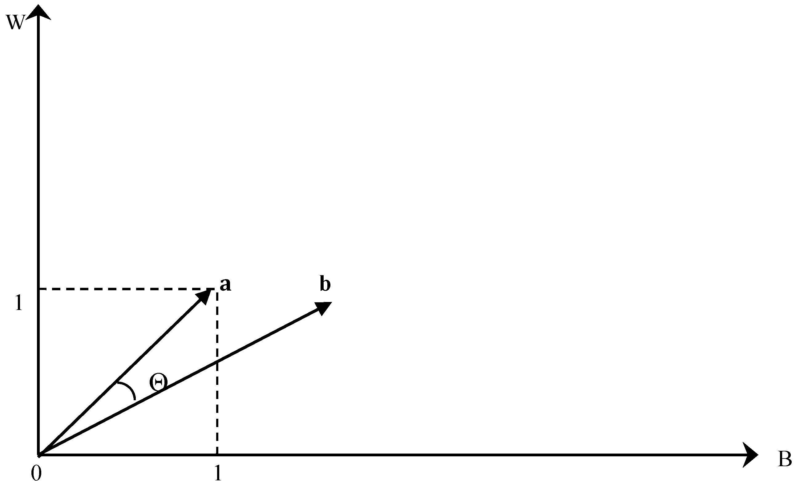
The methodology of measuring the structural composition of the beverages can be done by applying the methodology of angular separation. This is a general technique from trigonometry which measures the angle or distance between a set of vectors. The use of angular separation in economics can be found in [10], applied in relation to R&D topics, and also used by [11] concerning grape varieties, and finally, [9] uses the methodology for depicting similarity indices for alcohol consumption between countries. In the present analyses, we use angular separation for the measurement of the structural composition of alcohol consumption in any country. This is an absolute measure of the consumption structure and is further illustrated in Figure 1 for the case of two beverages, beer and wine.
The structural measure can be illustrated in the two-dimensional space where the alcohol consumption structure is defined by cosine to Θ from the graph. In the general case, with the three beverages, the angle between the vector b = (B, W, S) and a vector of unit values a = (1,1,1) will indicate the skewness of actual consumption relative to a case where the beverages are consumed in equal amounts.
The structural component will be defined from the dot product between a and b, and the length of the vectors:
The concept can be expanded to the n-dimensional space for the measure of angular separation, and with no obvious graphical exposition when n exceeds 3. In the present case with wine, beer and spirits, n equals 3 and the structural component calculated from (3) is simplified due to unit values in the vector a, and becomes
If the alcohol consumption is evenly distributed between beer, wine and spirits, then AS equals 1. The lower bound for AS is 3(−1/2), which is the value when consumption of two out of the three beverages approaches zero. Combining (1), (2) and (4) gives:
Consequently, the total consumption of alcohol (A) can be decomposed into a component representing the length (AL) of the beverage vector b and a structural component (AS) having a value between 3(−1/2) and unity.
As noted in the introduction, the primary aim of this paper is to analyze changes in the alcohol consumption structure, and therefore the next step is to set up a model explaining the structural component. In (6), we use traditional arguments as GDP per capita and trade openness, and additionally we have some control variables (Zi). The latter variables are the level of alcohol consumption, the share of rural population, tourist expenditures abroad and dummy variables to characterize the countries as historically so-called beer, wine or spirits countries.
AS = f(GDP/capita; Export/GDP-ratio; Zi)
In line with other convergence studies, it is expected that, within as well as between countries, GDP/capita has a positive influence on the structure of alcohol consumption in the direction of a more even structure. Furthermore, it is expected that ‘between differences’ for countries decrease as the income level increases. However, the influence from trade openness may be either positive or negative. For countries with a highly skewed alcohol consumption structure, a more open economy may open up for imports of other beverages—e.g., wine imports in the Nordic countries since the 1960s—and thus a more even structure of alcohol consumption. Still, trade may also cause vertical substitution, meaning that countries with preferences for e.g., beer continue to drink beer and increase the import of beer, resulting in a more skewed drinking pattern.
4. Data
The data to be used in the analyses come from various sources. Information on the alcohol consumption, i.e., wine, beer and spirits measured in 100% alcohol equivalents comes from the World Health Organization (the WHOSIS database) and from World Drink Trends (1999, 2005). This part of the data set covers the period 1960/1961 to 2014. Secondly, the national account variables such as per capita GDP and trade openness (export as per cent of GDP) are an extract from the OECD National Accounts, and World Development Indicators databases for the share of the population living in rural areas. Not all variables are available for the whole-sample period and for all countries, but the alcohol variables more or less cover all of the period 1960–2014. In order to pool data, GDP has to be measured in the same currency, which in the present case will be purchasing power parity data from OECD. Table 1 gives summary statistics for consumption.
In order to gain further insight into the dynamics of alcohol consumption and take into account e.g., historical and cultural differences, the countries are classified after the share of alcohol type preferred around the beginning of the 1960s. Thereby the twenty-one countries are separated into initial beer, wine or spirits-drinking countries with the numbers being 11, 6 and 4, respectively. Table 1 gives summary statistics for all 21 countries included in the sample and each of the three above mentioned country groups calculated at the start of the period, i.e., average values for 1961 to 1963. The drinking patterns were significantly different between countries classified as wine, beer or spirits-oriented. The share of beer was more than two-thirds in beer drinking countries, and wine had an even larger share: seventy per cent in the wine-drinking countries at the beginning of the 1960s. It is also noteworthy that the share of wine in spirits-oriented countries was less than twelve percent. Initially, the total alcohol consumption per inhabitant (+15 years) varied significantly between the three groups of countries with by far the highest consumption level in the traditional wine countries. The beer and spirits-oriented countries have increased their consumption level while the opposite has taken place in the initially wine-oriented countries, meaning that differences in the average alcohol consumption to a large extent have vanished between the three groups of countries.2
5. Convergence in the Alcohol Consumption Structure
By using Equation (4), Table 2 includes the results from calculating AS for the years 1961 and 2014 for the 21 OECD countries.
For almost all cases, the structural variable (AS) has increased in value, indicating a strong tendency towards more even alcohol consumption patterns. As compared to the significant differences in the beginning of the 1960s, there has been a clear case of convergence in the consumption patterns over time. Furthermore, this development has taken place towards a more balanced consumption pattern in most of the countries, and the values for AS in 2014 ranges between 0.82 and 0.99—except for the atypical development in Japan.
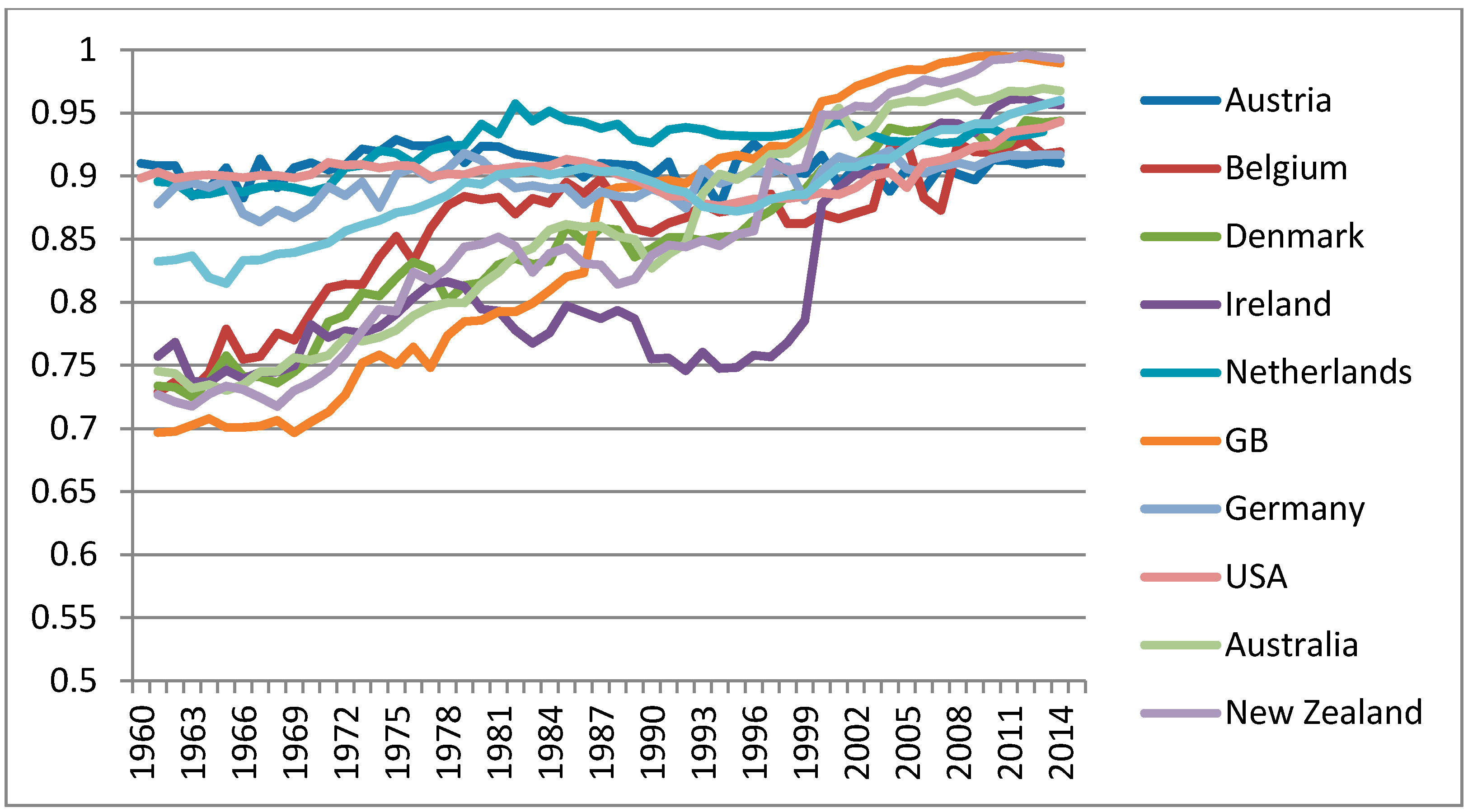
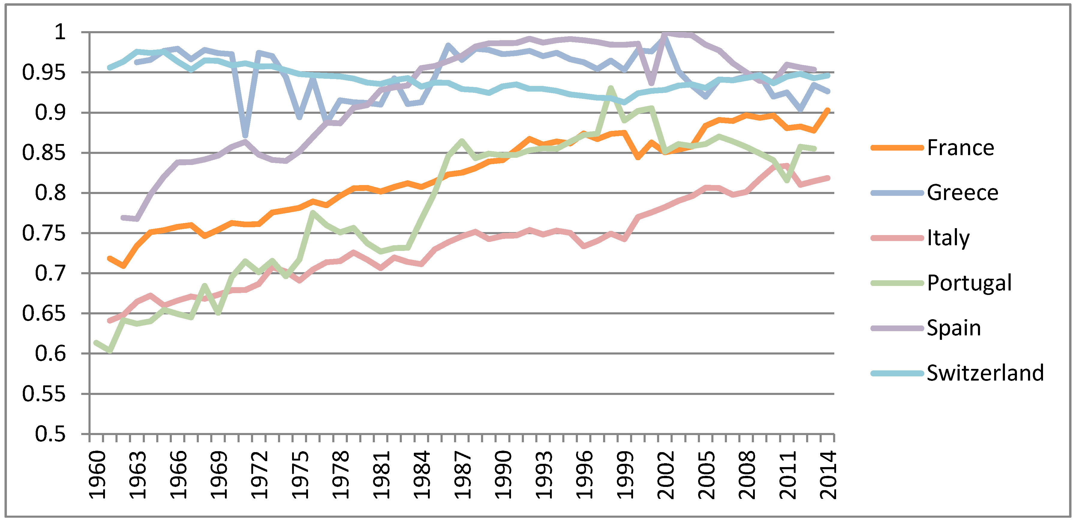
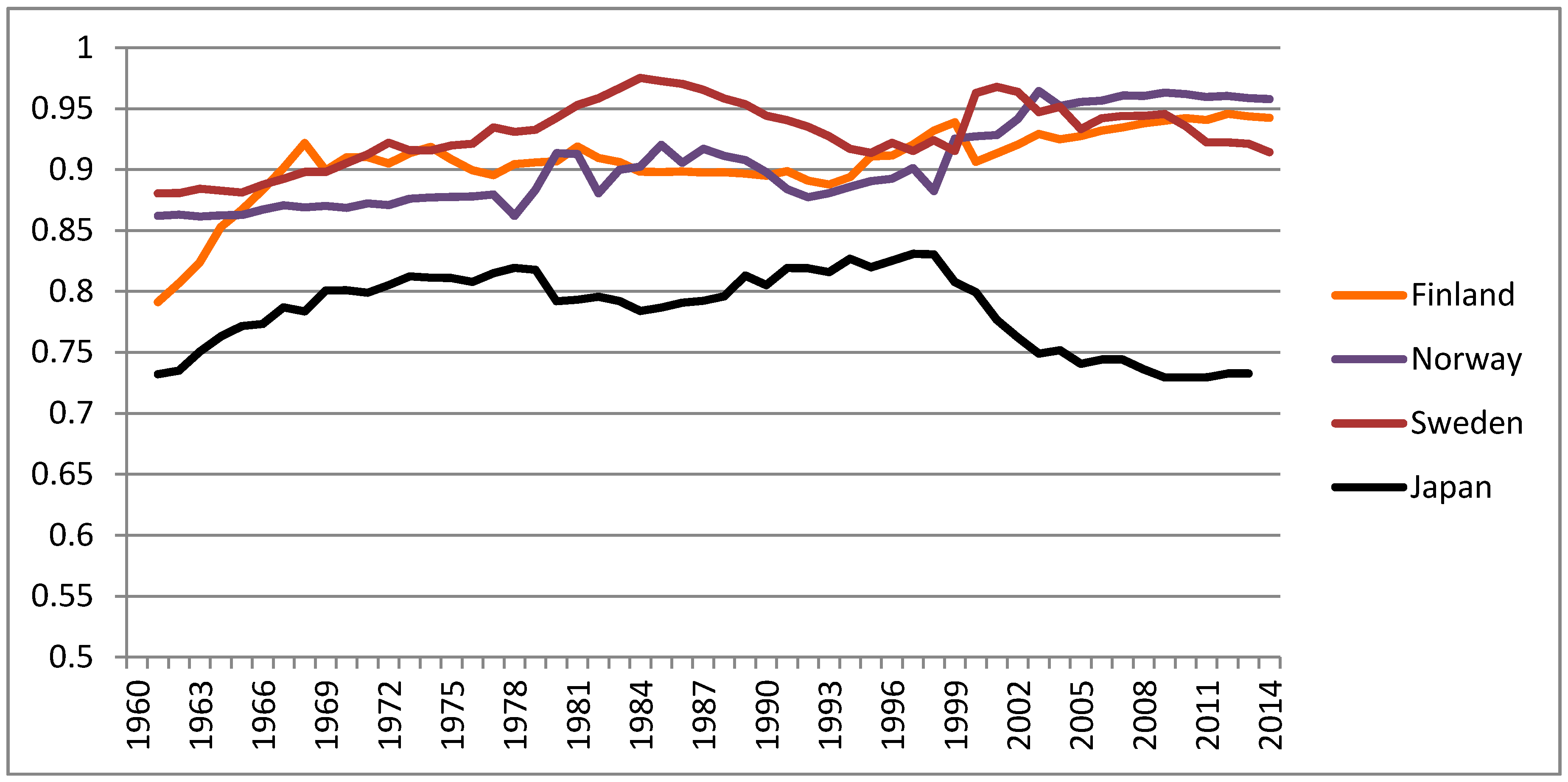
As metioned above, the countries are classified after the share of alcohol preferred at the beginning of 1966, see Table 1. Thereby the 21 countries are separated into initially beer, wine and spirits-oriented countries. Figure 2, Figure 3 and Figure 4 show the development in the alcohol consumption structure (AS) for each of these groups.
Focussing on the countries which initially were beer-oriented countries, there is a very clear tendency towards a more balanced alcohol consumption.3 The main explanation is the growth in wine consumption and a diminishing share of beer consumption. For most countries, the share of spirits is relatively constant over time and it is remarkable that As ends between 0.91 (Austria) and 0.99 (UK and New Zealand) for all countries, i.e., the underlying factors of influence in demand may have worked in similar fashions for all the initial beer oriented countries. Accordingly, the results indicate that within as well as between varation in drinking patterns vanish over time.
For the group of countries who are defined as initially wine-oriented countries, the same tendency can be seen in Figure 3, however to a lesser degree. Greece and Switzerland are dissimilar to the other countries, which is mainly due to a more balanced drinking pattern from the very beginning. However, looking at the traditional wine-producing countries, the within differences become smaller. The picture is less clear when comparing across countries. Obviously, Spain has an atypical development as compared to the other countries in this group, but the same can to a certain degree be seen for Portugal.
The third group of countries is the so-called spirits-oriented countries shown in Figure 4. Except for Denmark, this group consists of the Nordic countries, which are quite homogenous in many aspects: culture, living condition etc. Obviously, Japan is totally different from these three countries and with no tendency of convergence to a balanced drinking pattern; cf. also Table 2 with the still very low share of wine consumption.
Focussing solely on the Nordic countries, it is well known that sales of alcohol have been restricted to special state-owned liquor stores that are state monopolies. During recent years, the alcohol policies in the three countries have been lessened, meaning that normal beer can be bought in groceries and other retail shops, and furthermore, the supply of wine in the state monopoly stores has become much more varied.
6. Results
The theoretical model for the alcohol consumption structure (AS) is estimated from the data discussed in Section 3 above. The estimation period covers a more than 50 year long time span, which is remarkable. All the parameters presented in Table 3 are the results of fixed effect estimations which eliminate some of the between country differences—the table reports the final model,4 including four explanatory variables.
First of all, the per capita income is chosen because higher levels of income facilitate changes in the demand structure; i.e., the income elasticity of demand cannot be assumed to be negligible and the same for various kinds of alcohol, see the discussion above. The estimation results give support to this viewpoint. Looking at the first column, per capita GDP has a notable positive influence on AS, which means that increasing population income tends to even out the alcohol consumption with respect to beer, wine and spirits. Moreover, the influence from income on AS is largest for the initial beer-drinking countries (column 2), which is consistent with the empirical evidence that the income elasticity for beer is smaller than for wine. Income does not seem to influence changes in the alcohol consumption structure in especially spirits drinking countries (column 4) suggesting that tradition plays a larger role in these cases.
Note that, as mentioned, above the per capita income is measured by GDP in PPP terms. A particular issue that has to be addressed is how to deal with the choice of currency for the various countries. Additionally, pooling data without including fixed effects in the estimation model would obviously result in parameter values which depend on the units of the respective country currencies. This calls for using a common standard, such as measuring GDP for all countries in constant PPP dollar terms. However, such a procedure is problematic because it may create noise in the within country dynamics of real income.
Secondly, in line with [14], trade openness is included in the model. Thus, a tradition for high levels of trade facilitates and opens up a more differentiated supply of goods. Supply of alcohol is a unique example for many countries, e.g., Denmark, which is an open, wine-importing economy and thereby creates a high level of wine consumption, despite not being a wine-producing country.
Trade openness is measured by the export share or more precisely the total export value divided by GDP. We expect open economies to be potentially more inclined to changes in demand. However, despite being significant, the estimated parameters across beer, wine and spirits-oriented countries are very small. The negative sign of the parameters point in the direction of vertical substitution of the already preferred alcohol type.
Alcohol consumption per capita (+15 year) is clearly a driver of convergence in the alcohol consumption structure. Thus, for beer-oriented countries, the estimated parameter is positive and highly significant, suggesting that the increase in alcohol consumption over time (see Table 1) has facilitated structural changes towards a more even alcohol consumption structure. The negative parameter for initial wine-oriented countries reflects the fact that this country group has lowered its alcohol consumption considerably since the beginning of the 1960s; see Table 1. Thus, during the process of adjustment of the consumption level, more even drinking patterns have developed.
Finally, various control variables for other factors that may influence alcohol consumption patterns have been tested. A demographic parameter showing the share of people living in a rural area has been maintained in Table 3 with significant parameter estimates. Another candidate for measuring the impact of an open economy on drinking patterns is the share of household final consumption expenditures that take place abroad. Unfortunately, this will reduce the data set considerably, as the data do not go that far back in time and are not included in the model5 presented in Table 3.
7. Conclusions
Since the 1960s, there has been a strong tendency for convergence in alcohol consumption patterns among OECD countries, with more even or similar drinking patterns. This relates to both the levels of alcohol consumption as well as structural changes concerning more even shares of beer, wine and spirits. It has to a high degree been influenced by the consumption of wine, where wine-producing countries have experienced declining wine consumption, with the opposite tendency for the initially beer-drinking countries. Thus, a common feature seems to be a movement towards a more balanced structure of alcohol consumption in the OECD area. This is most likely driven by the development in real incomes—i.e., economic growth and convergence also have impacts on consumption patterns—but also factors such as trade openness and demographics are found to have significant influence, along with the overall level of alcohol consumption. Alcohol taxes and prices of the respective beverages must be expected to be influential on the consumption patterns, but data on such parameters are generally not available, thereby leaving this topic to be addressed in future research.
Author Contributions
Both authors contributed equally to the manuscript.
Conflicts of Interest
The authors declare no conflict of interest.
References
- Colen, L.; Swinnen, J. Economic Growth, Globalisation and Beer Consumption. J. Agric. Econ. 2016, 67, 186–207. [Google Scholar] [CrossRef]
- Nelson, J.P. Robust Demand Elasticities for Wine and Distilled Spirits: Meta-Analysis with Corrections for Outliers and Publication Bias. J. Wine Econ. 2013, 8, 294–317. [Google Scholar] [CrossRef]
- Selvanathan, S.; Selvanathan, E. Another look at the identical tastes hypothesis on the analysis of cross-country alcohol data. Empir. Econ. 2007, 32, 185–215. [Google Scholar] [CrossRef]
- Selvanathan, S. How similar are alcohol drinkers? International evidence. Appl. Econ. 2006, 38, 1353–1362. [Google Scholar] [CrossRef]
- Deaton, A.; Muellbauer, J. An Almost Ideal Demand System. Am. Econ. Rev. 1980, 70, 312–326. [Google Scholar]
- Bentzen, J.; Eriksson, T.; Smith, V. Alcohol Consumption in the European Countries: A time series based test of convergence. Cah. Econ. Sociol. Rural. 2001, 60, 59–74. [Google Scholar]
- Bentzen, J.; Smith, V. Developments in the Structure of Alcohol Consumption in OECD Countries; Wine Economics Workshop: Adelaide, Australia, 2010. [Google Scholar]
- Bentzen, J.; Smith, V. An analysis of structural changes in the consumption patterns of beer, wine and spirits applying an alternative methodology. In Proceedings of the XXIV EuAWE Conference, Bologna, Italy, 7–9 June 2017; Available online: http://www.vdqs.net/2017Bologna/DOCuments/Publications/text/6A_Bentzen_Smith.pdf (accessed on 7 June 2017).
- Holmes, A.J.; Anderson, K. Convergence in National Alcohol Consumption Patterns: New Global indictors. J. Wine Econ. 2017, 12, 117–148. [Google Scholar] [CrossRef]
- Jaffe, A.B. Real Effects of Academic Research. Am. Econ. Rev. 1989, 79, 957–970. [Google Scholar]
- Anderson, K. Terroir rising? Varietal and quality distinctiveness of Australia’s wine regions. Enometrica 2009, 2, 9–27. [Google Scholar]
- Colen, L.; Swinnen, J. Beer drinking nations—The determinants of global beer consumption. In AAWE Working Paper; Economics Department, New York University: New York, NY, USA, 2011; p. 79. [Google Scholar]
- Devaux, M.; Sassi, F. Alcohol consumption and harmful drinking: Trends and social disparities across OECD countries. In OECD Health Working Papers; OECD Publishing: Paris, France, 2015; p. 79. [Google Scholar]
- Kossova, T.; Kossova, E.; Sheluntcova, M. Investigating the volume and structure of alcohol consumption in Russians regions. J. Econ. Stud. 2017, 44, 266–281. [Google Scholar] [CrossRef]
- Lee, J.-H. The Influence of Alcohol Consumption on Income and Health: Empirical Evidence from a Panel of OECD Countries. Seoul J. Econ. 2013, 26, 25–282. [Google Scholar]
- Nelson, J.P. Alcohol advertising bans, consumption and control policies in seventeen OECD countries, 1975–2000. Appl. Econ. 2010, 42, 803–823. [Google Scholar] [CrossRef]
| 1 | |
| 2 | See also [6] for a time series based test of convergence in alcohol consumption. |
| 3 | The atypical development in Ireland is due to a large drop in the wine share in 2000 and a similar increase in the spirits share. |
| 4 | In the experimental phase, a number of other variables were included in the models. Per capita final consumption expenditure of resident households on the territory and abroad were included as an alternative to per capita GDP, and furthermore, final consumption expenditures of resident households abroad were tried in order to account for openness of the economy. However, when including these variables, the data set will be shortened considerably. |
| 5 | The share of consumption spend abroad might replace the export/GDP-share in the model as a measure of openness. |
Figure 1.
Measuring the beverage structure: Cos Θ.

Figure 2.
The structure of alcohol consumption in beer-oriented countries, 1960–2014. Note: The structural variable calculated from Equation (4).
Figure 2.
The structure of alcohol consumption in beer-oriented countries, 1960–2014. Note: The structural variable calculated from Equation (4).

Figure 3.
The structure of alcohol consumption in wine drinking countries, 1960–2014. Note: The structural variable calculated from the Equation (4).
Figure 3.
The structure of alcohol consumption in wine drinking countries, 1960–2014. Note: The structural variable calculated from the Equation (4).

Figure 4.
The structure of alcohol consumption in spirits drinking countries, 1960–2014. Note: The structural variable calculated from the Equation (4).
Figure 4.
The structure of alcohol consumption in spirits drinking countries, 1960–2014. Note: The structural variable calculated from the Equation (4).


Table 1.
Summary statistics for wine, beer and spirits shares in total alcohol consumption measured in pure alcohol equivalents, average 1961–1963 and total alcohol consumption 1961–1963; 2013–2014.
Table 1.
Summary statistics for wine, beer and spirits shares in total alcohol consumption measured in pure alcohol equivalents, average 1961–1963 and total alcohol consumption 1961–1963; 2013–2014.
| Variable | Mean | Std. Dev. | Minimum | Maximum |
|---|---|---|---|---|
| All countries | ||||
| Beer | 0.448 | 0.269 | 0.019 | 0.812 |
| Wine | 0.269 | 0.304 | 0.007 | 0.930 |
| Spirits | 0.283 | 0.193 | 0.050 | 0.738 |
| Alcohol consumption, avg. 1961–1963 | 9.616 | 5.457 | 3.000 | 25.09 |
| Alcohol consumption, avg. 2013–2014 | 9.301 | 1.618 | 6.140 | 12.18 |
| Beer-oriented countries | ||||
| Beer | 0.661 | 0.133 | 0.469 | 0.812 |
| Wine | 0.108 | 0.079 | 0.041 | 0.313 |
| Spirits | 0.231 | 0.117 | 0.112 | 0.436 |
| Alcohol consumption, avg. 1961–1963 | 8.026 | 2.064 | 4.297 | 11.97 |
| Alcohol consumption, avg. 2013–2014 | 10.027 | 1.348 | 8.150 | 12.18 |
| Wine-oriented countries | ||||
| Beer | 0.137 | 0.134 | 0.019 | 0.358 |
| Wine | 0.697 | 0.215 | 0.429 | 0.930 |
| Spirits | 0.166 | 0.097 | 0.050 | 0.316 |
| Alcohol consumption, avg. 1961–1963 | 16.136 | 5.439 | 9.827 | 25.09 |
| Alcohol consumption, avg. 2013–2014 | 9.188 | 1.490 | 7.460 | 11.30 |
| Spirits-oriented countries | ||||
| Beer | 0.329 | 0.121 | 0.202 | 0.466 |
| Wine | 0.070 | 0.050 | 0.007 | 0.123 |
| Spirits | 0.602 | 0.125 | 0.478 | 0.738 |
| Alcohol consumption, avg. 1961–1963 | 4.208 | 1.310 | 3.000 | 6.057 |
| Alcohol consumption, avg. 2013–2014 | 7.472 | 1.129 | 6.140 | 8.890 |
Table 2.
The structure of alcohol consumption (AS) and the share of wine, 1961 and 2014.
| Structure (AS) | Share of Wine | |||
|---|---|---|---|---|
| 1961 (1) | 2014 (2) | 1961 (3) | 2014 (4) | |
| Austria | 0.97 | 0.91 | 0.29 | 0.35 |
| Belgium | 0.73 | 0.92 | 0.13 | 0.36 |
| Denmark | 0.73 | 0.94 | 0.08 | 0.45 |
| Finland | 0.79 | 0.94 | 0.11 | 0.19 |
| France | 0.72 | 0.90 | 0.79 | 0.56 |
| Germany | 0.88 | 0.92 | 0.17 | 0.28 |
| Greece | 0.87 | 0.93 | 0.55 | 0.52 |
| Ireland | 0.76 | 0.96 | 0.06 | 0.26 |
| Italy | 0.64 | 0.82 | 0.90 | 0.66 |
| Netherlands | 0.90 | 0.94 | 0.10 | 0.34 |
| Norway | 0.86 | 0.96 | 0.06 | 0.37 |
| Portugal | 0.62 | 0.86 | 0.94 | 0.61 |
| Spain | 0.72 + | 0.95 * | 0.77 | 0.22 * |
| Sweden | 0.78 | 0.91 | 0.09 | 0.49 |
| Switzerland | 0.94 | 0.95 | 0.47 | 0.48 |
| UK | 0.70 | 0.99 | 0.04 | 0.39 |
| USA | 0.90 | 0.94 | 0.11 | 0.18 |
| Canada | 0.83 | 0.96 | 0.06 | 0.25 |
| Australia | 0.75 | 0.97 | 0.10 | 0.37 |
| New Zealand | 0.73 | 0.99 | 0.04 | 0.35 |
| Japan | 0.77 | 0.73 * | 0.01 | 0.05 * |
Notes: Alcohol consumption is the number of (pure) alcohol liters per inhabitant (+15 years). + data from 1962; * data for 2013. Source: The World Health Organization (the WHOSIS database). World Drink Trends (1999, 2005).
Table 3.
Regression models: the structural variable of alcohol consumption variable (AS).
| All Countries (1) | Beer Drinking Countires (2) | Wine Drinking Countries (3) | Spirits Drinking Countries (4) | |
|---|---|---|---|---|
| Per capita GDP (logs) | 0.1719 * (0.0079) | 0.2198 * (0.0107) | 0.1115 * (0.014) | 0.0786 * (0.0128) |
| Trade openness export/GDP | −0.0004 * (0.0001) | −0.0009 * (0.0002) | −0.0009 * (0.0002) | −0.0004 (0.0002) |
| Share of population living in rural areas | 0.0031 * (0.0005) | 0.0025 * (0.0007) | −0.0008 * (0.0006) | 0.0034 * (0.0007) |
| Alcohol consumption (pure alcohol litres per inhabitant, +15 years). | −0.0254 (0.0081) | 0.0629 * (0.0145) | −0.0734 * (0.0147 | 0.0004 * (0.0147) |
| R-squared | 0.75 | 0.67 | 0.91 | 0.86 |
| Regression F Significance | 121.2 * 0.000 | 74.4 * 0.000 | 285.5 * 0.000 | 153.7 * 0.000 |
| Observations | 963 | 516 | 268 | 179 |
Notes: OLS estimation by fixed effects (21 countries). Standard errors in brackets below the estimated parameters. * denotes significance at the 1% level.
© 2018 by the authors. Licensee MDPI, Basel, Switzerland. This article is an open access article distributed under the terms and conditions of the Creative Commons Attribution (CC BY) license (http://creativecommons.org/licenses/by/4.0/).
Share and Cite
MDPI and ACS Style
Bentzen, J.; Smith, V. Structural Changes in the Consumption of Beer, Wine and Spirits in OECD Countries from 1961 to 2014. Beverages 2018, 4, 8. https://0-doi-org.brum.beds.ac.uk/10.3390/beverages4010008
AMA Style
Bentzen J, Smith V. Structural Changes in the Consumption of Beer, Wine and Spirits in OECD Countries from 1961 to 2014. Beverages. 2018; 4(1):8. https://0-doi-org.brum.beds.ac.uk/10.3390/beverages4010008
Chicago/Turabian StyleBentzen, Jan, and Valdemar Smith. 2018. "Structural Changes in the Consumption of Beer, Wine and Spirits in OECD Countries from 1961 to 2014" Beverages 4, no. 1: 8. https://0-doi-org.brum.beds.ac.uk/10.3390/beverages4010008
Note that from the first issue of 2016, this journal uses article numbers instead of page numbers. See further details here.