Geographical Classification of Tannat Wines Based on Support Vector Machines and Feature Selection

Abstract

Geographical product recognition has become an issue for researchers and food industries. One way to obtain useful information about the fingerprint of wines is by examining that fingerprint’s chemical components. In this paper, we present a data mining and predictive analysis to classify Brazilian and Uruguayan Tannat wines from the South region using the support vector machine (SVM) classification algorithm with the radial basis kernel function and the F-score feature selection method. A total of 37 Tannat wines differing in geographical origin (9 Brazilian samples and 28 Uruguayan samples) were analyzed. We concluded that given the use of at least one anthocyanin (peon-3-glu) and the radical scavenging activity (DPPH), the Tannat wines can be classified with 94.64% accuracy and 0.90 Matthew’s correlation coefficient (MCC). Furthermore, the combination of SVM and feature selection proved useful for determining the main chemical parameters that discriminate with regard to the origin of Tannat wines and classifying them with a high degree of accuracy. Additionally, to our knowledge, this is the first study to classify the Tannat wine variety in the context of two countries in South America.

1. Introduction

The contemporary global wine industry is inherently geographical, with the origins of the grapes being a main factor in the eminence of this particular beverage [1]. Additionally, customers are interested in finding high-quality wines that specify their geographical region [2]. In this regard, performing a fingerprinting approach to characterize wines and to classify their characteristics according to their production regions is a necessity. Tests to confirm the origin of a specific wine are necessary, because wine production and trade have always been associated with high costs [3]. Based on this background, detailed and continuous controls are essential for maintaining the quality of wine and for identifying possible cases of fraud with respect to their geographical origin [4].

Latin-American viticulture belong to the New World of wine, both in terms of productivity and levels of consumption [5]. Since the middle of the 19th century, Tannat has been the main variety of red wines cultivated in Uruguay [6]. This variety is adaptable to the ecological conditions of Uruguay, producing exceptional wines, highlighted by its originality [7]. In Brazil, a country new to wine production, Tannat is one of the six most cultivated varieties (along with Cabernet Franc, Cabernet Sauvignon, Merlot, Pinotage, Pinot Noir). Wine production has a significant economic and social impact on the southern region of Brazil, which represents 90% of wine production in that nation [8].

Unsupervised techniques, such as principal component analysis and cluster analysis, have commonly been employed to differentiate wines [9,10,11,12,13]. However, unsupervised pattern recognition methods must not be confused with classification methods. In some cases, these techniques allow for the identification and visualization of certain patterns, while in other cases, they may be insufficient for finding patterns between food profiles and physicochemical attributes, due to the multitude of compounds and physical attributes that are present in food products [14,15].

Other studies have used unsupervised techniques prior to using supervised techniques, such as linear discriminant analysis, partial least squares-discriminant analysis, and decision trees to classify wine samples [8,16,17,18]. In addition, other advanced techniques available through current data mining methodology have been successfully used to classify wines and other food products according to their geographical origin and variety, such as support vector machines (SVM) [19]. In addition, SVM is a suitable classifier for balanced datasets [20].

The SVM classification algorithm has been demonstrated to be useful for wine classification. For example, a total of 44 Polish white and red wine samples from different parts of Poland were classified [21]. The authors used principal component analysis (PCA) as an exploratory analysis and support vector machine method, with a radial basis function (RBF), to classify the data according to grape variety, geographic region, sugar content, alcohol content, type of yeast used, post-fermentation treatment, and the temperature in the fermentation process. The main results of this study of the classification of white and red wines, according to the variety of grapes used for production, showed 98.7 and 98.2% accuracy, respectively. SVM with an RBF kernel was compared to the partial least squares discrimination analysis (PLS-DA) to classify 1188 wine samples from South Africa, Hungary, Romania, and the Czech Republic [22]. Results showed that the SVM models, using 25 variables, have proven to be more efficient than the PLS-DA, with an accuracy of at least 95%. Another study compared SVM and PLS-DA in order to classify seventy-nine wine vinegar samples from three Spanish regions. The samples were classified according to their origin and their categories (aged and sweet), and the SVM classification models demonstrated a higher ability of prediction (between 92% and 100% correctly classified samples) than for the PLS-DA models [23].

A group of sixty-four samples of white wine belonging to four different Spanish DO (wine with designation of origin) were classified, based on SVM and linear discriminant analysis (LDA) [24]. The authors achieved an accuracy of 100% with the SVM model when using five selected variables, according to the Kruskal–Wallis test, the PCA, and the backward stepwise LDA. A previous study carried out by our group classified the geographical origin of Cabernet Sauvignon wines from Brazil and Chile with the use of SVM with an RBF kernel and correlation-based feature selection [25]. The results showed a good classification rate of 89% when using the 20 original elements, and an accuracy of 83% when using only five elements (L *, DPPH (2,2-diphenyl-1-picrylhydrazyl), delph-3-acetylglu, peon-3-(coum)glu, and pet-3-acetylglu). Another recent paper classified South America wines using SVM and other classifiers [26]. This study classified wines from Argentina, Chile, Brazil, and Uruguay based on their mineral content. The authors proposed a new feature selection method and had used SVM, LDA, neural networks, and Naïve Bayses, outperforming the other classifiers in all features, including the best feature, subset SVM.

The aim of this paper is to classify Tannat wines from the southern regions of Brazil and Uruguay, using data mining techniques. The contributions of this paper can be summarized as follows: 1) Analysis of the same wine variety from two different countries; 2) the possibility of irrelevant and redundant features of the wines′ chemical parameters, as associated with their functionality, designed as antioxidant activity (DPPH and ORAC), total polyphenols (TP), total anthocyanins (TA) and color, is taken into consideration to select an optimal subset of features for classification; and 3) the use of data mining techniques to classify wines.

2. Materials and Methods

2.1. Wine Samples

Tannat wine samples were obtained from local markets and wine distributers in the city of São Paulo (Brazil). All the wines are monovarietal (at least 75% of Tannat variety), from 2009 and 2010 vintages, bottled in 750 mL bottles, and with retail prices between 1–50 United States dollars (USD). Samples were distributed as follows: Uruguay (n = 28) and Brazil (n = 9).

2.2. Chemical Compounds Determination

The variables analyzed for each wine were: Color by CIELAB (L *, a *, b *), total polyphenols (TPI), total anthocyanins (TA), antioxidant activity by oxygen radical absorbance capacity (ORAC) and free radical scavenging activity (DPPH), and individual anthocyanins (cyan-3-glu, delph-3-acetylglu, delph-3-glu, malv-3-(coum)glu, malv-3-acetylglu, malv-3-glu, peon-3-(coum)glu, peon-3-acetylglu, peon-3-glu, pet-3-(coum)glu, pet-3-acetylglu, pet-3-glu, and vitisin A).

2.3. Color Determination

The analysis of color was performed by measuring the transmittance in a ColorQuest XE colorimeter (Hunter Associates Laboratory, Inc., Reston, VA, USA) using the CIE 1964 standard observer (10° visual field) and the CIE standard illuminant D65 as references. The software EasyMatch QC (Hunter Associates Laboratory, Inc., Reston, VA, USA) was used to determine the three CIELAB coordinates: a * (red-green; +a *, −a *), b * (yellow-blue; +b *, −b *), and lightness L * (white-black, 0–100). The analyses were performed in triplicate.

2.4. Total Polyphenols

Total polyphenols (TPI) were determined using the Folin–Ciocalteu colorimetric method [27]. This method was adapted for measurement with a microplate reader, employing a standard curve of gallic acid (ranging from 0 to 100 mg/L). The results are expressed as mg gallic acid equivalents per liter (mg GAE/L). The analyses were performed in triplicate.

2.5. Total Monomeric Anthocyanins

Total anthocyanins (TA) were quantified, as described by Fuleki and Francis [28] with some modifications, using Equation (1):

$$TA=\frac{\left[\left(A510-A700\right)pH 1.0- \left(A510-A700\right)pH 4.5\right]\times MV\times DF\times 103}{\epsilon }$$

(1)

in which A510 and A700 are the absorbance at 510 and 700 nm, respectively, MW is the molecular weight of cyanidin-3-glucoside (449.2), DF is the dilution factor (10), and ε represents the molar absorptive of cyanidin-3-glucoside (26,900). The results are expressed as mg of cyanidin-3-glucoside per liter (mg cyanidin-3-glu/L). The experiments were performed in duplicate.

2.6. Individual Anthocyanins

2.6.1. HPLC–DAD

Individual anthocyanins were determined by HPLC, using the method described by Boido et al. [29] with some modifications. The identification of the anthocyanins was performed by comparing the retention time for each peak with available standards and values obtained from the literature. Analyses by HPLC–MS were performed to confirm these results, as described below. The individual anthocyanins were quantified using calibration curves of malvidin-3-glucoside (0.1–7.0 mg/L and 7.1–200 mg/L) and the areas obtained in the high-performance liquid chromatography with a diode-array detector (HPLC-DAD) analysis. The results are expressed as milligrams of malvidin-3-glucoside per liter (mg malvidin-3-glu/L). The analyses were performed in duplicate.

2.6.2. HPLC–DAD–MS

A Shimadzu Prominence SPD-M20A liquid chromatograph (Shimadzu Co., Kyoto, Japan) that was connected via a UV cell outlet to a Bruker Esquire HCT ion trap mass spectrometer (BrukerDaltonics Inc., Billerica, MA, USA) was used for the analysis. The HPLC–DAD conditions were identical to those described in the previous section. The MS contained an electrospray ionization interface (ESI) and used nitrogen as the drying gas at a flow rate of 6.0 L/min. The pressure of the nebulizer was set at 25.0 psi. The capillary temperature was 280 °C. Spectra were recorded in a positive ion mode between m/z 50 and 1100. The mass spectrometer was programmed to perform a series of three consecutive scans: A full mass scan, an MS2 scan of the most abundant ions in the full mass scan, and an MS3 scan of the most abundant ions in the MS2 scan. The obtained data were analyzed using the Bruker Compass DataAnalysis 4.0 software (BrukerDaltonik GmbH, Bremen, Germany).

2.7. Antioxidant Activity

The in vitro antioxidant activity of the wines was determined using two methods: Measuring the free radical scavenging capacity (DPPH) and the oxygen radical absorbance capacity (ORAC).

2.7.1. Free Radical Scavenging Capacity (DPPH)

The method described by Arnous et al. [30] was used with some modifications. The antiradical activity (AAR) of each sample, expressed in millimolarTrolox equivalents (mM TRE), was calculated using Equation (2):

$$AAR=0.872\times In\left(\%\Delta A515\right)- 2.922,$$

(2)

where $In\left(\%\Delta A515\right)=\frac{\left[\left(A515,control-A515,t=150\right)\right]}{A515,control}\times 100$.

The absorbance was read at 515 nm using a UVmini-1240 UV-VIS spectrophotometer (Shimadzu Corporation, Kyoto, Japan). The equation was determined by linear regression (r² = 0.992) after the plotting of known Trolox solutions (0.25–1.50 mM) against concentration. The analyses were performed in duplicate.

2.7.2. Oxygen Radical Absorbance Capacity (ORAC)

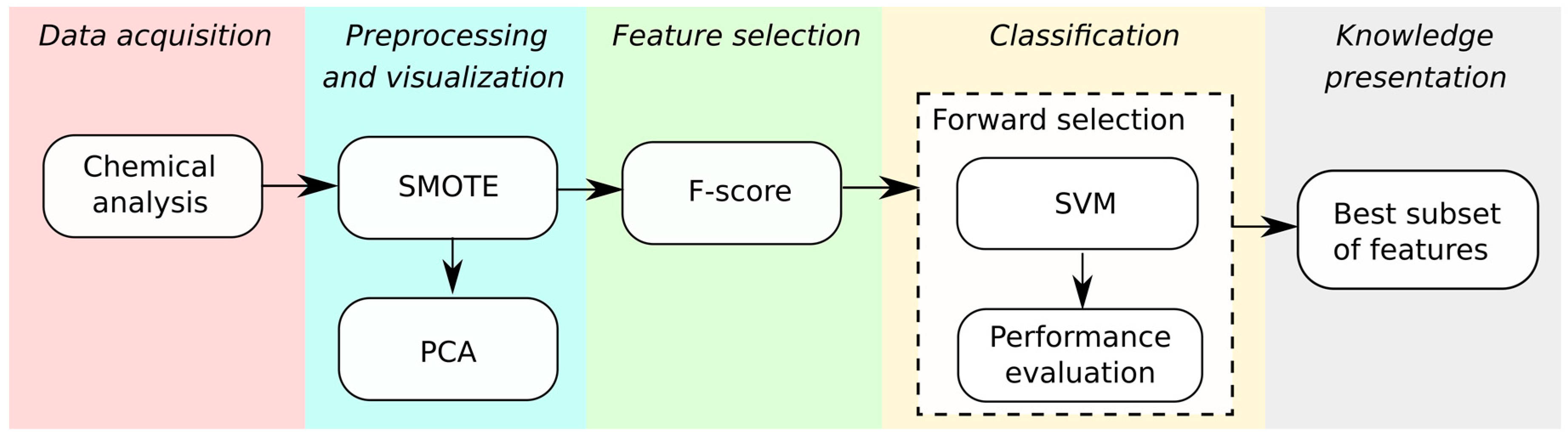
The ORAC assay was performed according to the method described by Huang et al. [31] with slight modifications. A calibration curve was prepared using known Trolox solutions (6.25–100 µM). The results are expressed as micromolar Trolox equivalents (µM TRE). Each sample was analyzed in quadruplicate.

2.8. Data Mining

Data mining is the process of automatic discovery of useful information in a database using a series of steps that can be carried out to discern these patterns [32]. These steps can be summarized as data cleaning (to remove noise and inconsistent data); data selection (whereby data relevant to the analysis are selected from the database); data transformation (whereby data are transformed by performing summary or aggregation operations; feature selection; or feature extraction); data mining (whereby machine learning algorithms are performed); pattern evaluation (identification of the interesting patterns based on performance measures); and finally, knowledge presentation.

In this study, we performed the data mining study as presented in Figure 1. The dataset is composed of 21 columns and 37 rows, including 20 columns that represent the chemical compounds, one column representing the class label (Brazil or Uruguay) and each row representing a wine sample. We used the synthetic minority over sampling technique (SMOTE) to create 19 new samples for the Brazilian class because an imbalanced dataset can benefit the majority class [33]. SMOTE is the most widely and effectively used oversampling method; it creates synthetic minority class samples by interpolating between real minority examples and their nearest neighbors.

After that, we visualized data through the use of PCA, a descriptive tool that visualizes the data in two dimensions. The F-score, a filter feature selection method, were used to rank features in the order of importance. According to the feature order generated, we constructed 20 feature subsets through an iterative forward-selection procedure. The feature with the highest F-score value was assigned to the first subset (#1). The top two features on the F-score ranking were assigned to the second subset (#2), and so on, until all features were assigned to the twentieth subset (#20).

The support vector machines classifier, with the radial basis function kernel, was used to build a classification model for each feature subset. This included a grid search on the classifier parameters for the leave-one-out cross-validation with training, validation, and test sets. Finally, four performance measures were computed for each model, based on the test set.

The entire analysis was conducted using R software [34]. R is a free software environment for statistical computing and graphics that contains a wide variety of packages for performing statistical analysis. In this study, we implemented the F-score algorithm and used the caret package [35] for data classification, as well as the ggplot2 package [36] to visualize some of the results.

2.9. Support Vector Machines

The support vector machine (SVM) [37] is a supervised learning model that analyzes data used for classification and regression analysis, based on the statistical learning theory and structural risk minimization. The algorithm used in this model obtains an optimal hyperplane with a maximum margin for separating the classes of samples. The generalization power with which the hyperplane separates the classes depends on its margin, defined as the distance between the hyperplane and the samples closest to it (support vector). This classifier is one of the most robust and accurate methods among the well-known data mining algorithms [38]. Additionally, it is a useful classification algorithm when few training data are available. It is also a suitable classifier for balanced datasets [20].

Given a two-class training set whose classes are linearly separable, i.e., all training samples can be correctly classified by the hyperplane, the algorithm computes the decision boundary based on samples that are closest to the maximum-margin hyperplane, which are called support vectors. This hyperplane is represented by Equation (3), in which w is a weight vector, x is the input data and b is a bias:

$$w·x+b=0$$

(3)

The goal is to maximize the margin of this hyperplane, increasing the distance between the samples within its limit. SVM finds an optimum separating hyperplane that maximizes the margin of the decision surface, by solving the following Equation (4):

$$\begin{gathered} \underset{w,b}{\min }\frac{1}{2}{w}^{t}w \\ s.t.y_i\left(w·x_i+b\right)-1\ge 0 \end{gathered}$$

(4)

However, in many real-world problems, it may not be possible to trace a decision boundary that separates the samples into the class labels. In these cases, it is necessary to apply a kernel function and to add slack variables. Thus, the SVM formulation becomes Equation (5):

$$\begin{gathered} \underset{w,b,{\xi }_i}{\min }\frac{{\parallel w\parallel }^2}{2}+C\left({\displaystyle \sum }_{i=1}^n{\xi }_i\right) \\ s.t. y_i\left(w·\varphi \left(x_i\right)+b\right)\ge 1-{\xi }_i, {\xi }_i\ge 0, i=1, \cdots , n. \end{gathered}$$

(5)

The kernel function Φ, based on the inner product between given data, performs a nonlinear transformation of data from the input space to a feature space with higher (even infinite) dimensions in order to make the problem linearly separable, as defined as Equation (6):

$$K\left(x_i, x_j\right)=\Phi \left(x_i\right)·\Phi \left(x_j\right)$$

(6)

In this study, we used the Gaussian radial basis function (RBF) kernel, defined by Equation (7):

$$K\left(x_i,x_j\right)=\exp \left(-\frac{\parallel x_i-x_j{\parallel }^2}{2{\sigma }^2}\right)$$

(7)

The C and σ parameters of Equations (5) and (7), respectively, are defined empirically, with a grid search taking place among the following values: C = 2^c, c = {−5, −3, …, 5}, and σ = 2^s, s = {−10, −8, …, 3}. Furthermore, RBF can produce a good performance, even when using a small number of samples [39].

2.10. Variable Selection

Variable selection methods provide a way of reducing computation time, improving prediction performance, and giving a better understanding of the data in machine learning applications [40]. To consider that there are possibly irrelevant or redundant variables in the data is important for improving the classification model. In this study, the F-score was employed to generate a ranking of importance [41]. The F-score is simple, generally quite effective, and has been used in previous studies [42,43,44,45]. Given training vectors $x_k, k=\left\{1,\dots , m\right\}$ and the number of positive and negative instances $n^{+}$ and $n^{-}$, respectively, the F-score of the i-th feature is defined by Equation (8):

$$F_i=\frac{\left({\overline{x}}_i^{+}-x_i\right)+\left({\overline{x}}_i^{-}-x_i\right)}{\frac{1}{n_{+}-1} {{\displaystyle \sum }}_{k=1}^{n^{+}}{\left({\overline{x}}_{k,i}^{(+)}-{\overline{x}}_i^{(+)}\right)}^2+\frac{1}{n_{-}-1} {{\displaystyle \sum }}_{k=1}^{n^{-}}{\left({\overline{x}}_{k,i}^{(-)}-{\overline{x}}_i^{(-)}\right)}^2},$$

(8)

where ${\overline{x}}_i, {\overline{x}}_i{}^{(+)}, \mathrm{and} {\overline{x}}_i{}^{(-)}$ are the average of the i-th feature of the whole, positive, and negative data sets, respectively; ${x_{ki}}^{(+)}$ is the i-th feature of the k-th positive instance, and ${x_{ki}}^{(-)}$ is the i-th feature of the k-th negative instance. The numerator indicates the discrimination between the positive and negative sets, and the denominator indicates the value within each of the two sets. The larger the F-score, the more likely that this feature will be more discriminative.

2.11. Performance Analysis

To evaluate the performance of a classification model, it is customary to split the data into two general parts, a training set and a test set, using holdout (70%–30%), 10-fold cross validation (k-fold CV), or leave-one-out cross validation (LOOCV) methodology. The holdout method is not indicated when the dataset has a small number of samples, making this method unfeasible in our study. Cross-validation is one possible solution for training and testing sets that have a small number of samples [32].

Due to our limited number of samples, a LOOCV strategy was employed to evaluate the performance of the classifier. This method is a particular case of the k-fold cross validation technique, which randomly splits data set D into k subsets D₁, D₂, …, D_k (the folds) of approximately equal size. In the LOOCV method, k is equal to the number of samples. The process of building the classification model occurs k times; the training set (k-1 folds) is used to perform the classification model, and the prediction ability was tested on the samples of the omitted fold. In the training phase, we performed an internal 10-fold cross-validation to validate the model and to select the best classifier parameters. This way, each sample was used to test the model without influencing the training phase, in order to avoid the introduction of bias.

After performing the classification models, it was possible to estimate the accuracy and percentage of correct predictions for each class of data. The results of the classification are established in a confusion matrix, as shown below in

Table 1. Confusion matrix example.

Reference	Prediction
	Positive	Negative
Positive	TP	FN
Negative	FP	TN

.

Interpreting the confusion matrix as presented with the data analyzed, we see that the positive samples (+) are from Brazil and the negative samples (−) are from Uruguay. The matrix values are true positive (TP) for samples correctly classified as positive, true negative (TN) for samples correctly classified as negative, false negative (FN) for the positive samples that were classified as negative, and false positive (FP) for negative samples that were classified as positive. From these values, we see that it is possible to establish the performance measures used in this study. The higher these parameters, the better the result:

$$\mathrm{Accuracy}=\frac{\mathrm{TP}+\mathrm{TN}}{\mathrm{TP}+\mathrm{TN}+\mathrm{FP}+\mathrm{FN}}\times 100,$$

(9)

$$\mathrm{Sensitivity}=\frac{\mathrm{TP}}{\mathrm{TP}+\mathrm{FN}}\times 100,$$

(10)

$$\mathrm{Specificity}=\frac{\mathrm{TN}}{\mathrm{TN}+\mathrm{FP}}\times 100,$$

(11)

$$\mathrm{MCC}=\frac{\mathrm{TP}\times \mathrm{TN}-\mathrm{FP}\times \mathrm{FN}}{\sqrt{\left(\mathrm{TP}+\mathrm{FP}\right)\left(\mathrm{TP}+\mathrm{FN}\right)\left(\mathrm{TN}+\mathrm{FP}\right)\left(\mathrm{TN}+\mathrm{FN}\right)}}.$$

(12)

The accuracy reflects how closely the classifier reaches its goal, that is, the accuracy mirrors the percentage of the model that has been correct in its predictions. Sensitivity refers to the percentage of correct answers with regard to the positive samples. Specificity is the opposite of sensitivity. It measures the percentage of samples correctly classified as negative. The Matthew’s correlation coefficient (MCC) is, in principle, a correlation coefficient that lies between the real class and the predicted class for binary classifications. The MCC returns a value between −1 and +1, where +1 represents a perfect prediction, −1 indicates total disagreement between prediction and the reference, and 0 means no better than random prediction.

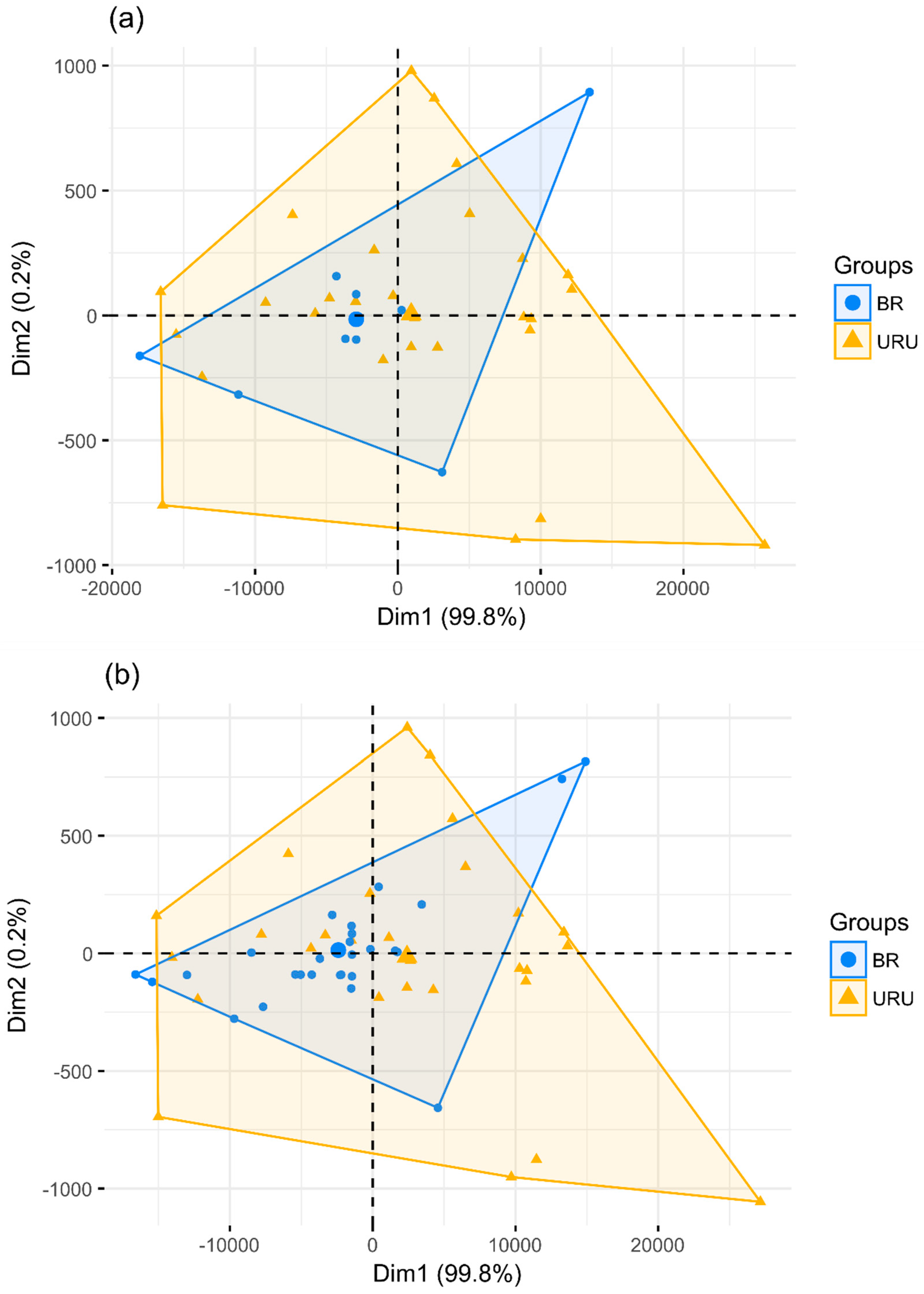
3. Results and Discussion

The methodology starts with the creation of new synthetic data, followed by the application of the feature selection method F-score on all features in order to generate a ranking of importance.

Table 2. Values of mean, standard deviation, and minimum and maximum variable concentration for each country.

Variable	Brazil (n = 28)	Uruguay (n = 28)
L *	16.02 ± 5.91 (3.84–31.02)	17.48 ± 6.25 (4.7–32.43)
a *	45.47 ± 6.74 (25.7–54.17)	47.24 ± 5.84 (29.43–54.51)
b *	26.35 ± 8.63 (6.37–42.87)	28.95 ± 9.59 (7.61–48.6)
TPI	1924.45 ± 352.61 (1365.36–2999.55)	1973.45 ± 454.56 (1015.98–2946.75)
TA	143.41 ± 35.32 (95.35–233.45)	117.02 ± 52.93 (28.72–289.56)
ORAC	39,623.59 ± 6942.55 (25,423.23–56,914.9)	44,431.93 ± 9938.45 (26,883.63–69,192.46)
DPPH	8.88 ± 0.58 (7.55–9.82)	9.56 ± 0.67 (7.12–10.34)
cyan-3-glu	0.22 ± 0.12 (0.1–0.62)	0.18 ± 0.07 (0.07–0.36)
delph-3-acetylglu	1.15 ± 0.81 (0.48–3.61)	0.98 ± 0.7 (0.33–3.83)
delph-3-glu	6.19 ± 2.71 (2.17–11.38)	3.65 ± 2.63 (0.29–11.4)
malv-3-(coum)glu	6.36 ± 2.89 (2.97–11.84)	5.04 ± 3.53 (0.41–14.18)
malv-3-acetylglu	13.05 ± 5.69 (4.55–27.78)	11.01 ± 7.35 (1.04–30.79)
malv-3-glu	42.58 ± 22.03 (26.03–95.19)	36.89 ± 22.79 (3.86–89.98)
peon-3-(coum)glu	1.48 ± 1.98 (0.57–4.71)	1.76 ± 2.07 (0.27–11.11)
peon-3-acetylglu	1.57 ± 0.74 (0.89–3.25)	1.41 ± 0.61 (0.51–2.9)
peon-3-glu	4.27 ± 2.12 (1.61–9.99)	2.11 ± 1.46 (0.4–5.72)
pet-3-(coum)glu	0.45 ± 0.56 (0.1–2.14)	0.28 ± 0.29 (0.1–1.64)
pet-3-acetylglu	2.43 ± 2.02 (1.04–8.63)	1.57 ± 1.74 (0–9.1)
pet-3-glu	11.02 ± 3.97 (4.98–22.14)	7.16 ± 5.21 (0.46–24.52)
vitisin A	14.37 ± 5.2 (5.37–22.25)	11.32 ± 8.89 (1.95–43.75)

describes the interval of concentrations for each variable. An exploratory PCA shown in Figure 1 reveals that the two classes of wines cannot be differentiated. The PC1–PC2 scores′ subspace accounted for 100% of the original variance. Figure 2a shows the original data and Figure 2b reveals the dataset resulting from the combination of the original data and 19 new synthetic samples. The new samples occupied the same region on the PCA plot as the original samples.

3.1. Classification Analysis

At first, we classified only the original samples in order to obtain a reference result for comparing this outcome with the balanced dataset results. The classification model with all features along with LOOCV resulted in the following performance measures: 72.97% of accuracy, an MCC of 0.45, a sensitivity of 40%, and 78.12% of specificity. These results indicate that the few Brazilian samples could be poorly classified, and that the model benefited the majority class. In addition, the MCC metric indicates that the predictions were closer to being random than perfect predictions.

The next step was to generate the ranking of importance and perform the classification models. Figure 3 shows the F-score ranking of importance. Then, we constructed 20 feature subsets, an iterative forward-selection procedure based on the F-score ranking of importance. The first feature subset (#1) is composed of the peon-3-glu compound; the second feature subset (#2) is composed of the peon-3-glu and DPPH parameters, and so forth; until the twentieth feature subset (#20), which is composed of all the parameters.

Table 3. Overall results from leave-one-out cross validation (LOOCV) classification with the support vector machine (SVM) for each feature subset.

#	Compounds	Acc	MCC	Sens	Spec
#1	peon-3-glu	91.07	0.82	89.66	92.59
#2	peon-3-glu, DPPH	94.64	0.90	90.32	100
#3	peon-3-glu, DPPH, delph-3-glu	85.71	0.71	85.71	85.71
#4	peon-3-glu, DPPH, delph-3-glu, pet-3-glu	92.86	0.86	90.00	96.15
#5	peon-3-glu, DPPH, delph-3-glu, pet-3-glu, TA	91.07	0.82	89.66	92.59
#6	peon-3-glu, DPPH, delph-3-glu, pet-3-glu, TA, ORAC	94.64	0.90	90.32	100
#7	peon-3-glu, DPPH, delph-3-glu, pet-3-glu, TA, ORAC, pet-3-acetylglu	91.07	0.83	87.10	96.00
#8	peon-3-glu, DPPH, delph-3-glu, pet-3-glu, TA, ORAC, pet-3-acetylglu, vitisin A	94.64	0.90	90.32	100
#9	peon-3-glu, DPPH, delph-3-glu, pet-3-glu, TA, ORAC, pet-3-acetylglu, vitisin A, cyan-3-glu	91.07	0.83	87.10	96.00
#10	peon-3-glu, DPPH, delph-3-glu, pet-3-glu, TA, ORAC, pet-3-acetylglu, vitisin A, cyan-3-glu, malv-3-(coum)glu	91.07	0.83	87.10	96.00
#11	peon-3-glu, DPPH, delph-3-glu, pet-3-glu, TA, ORAC, pet-3-acetylglu, vitisin A, cyan-3-glu, malv-3-(coum)glu, pet-3-(coum)glu	85.71	0.72	83.33	88.46
#12	peon-3-glu, DPPH, delph-3-glu, pet-3-glu, TA, ORAC, pet-3-acetylglu, vitisin A, cyan-3-glu, malv-3-(coum)glu, pet-3-(coum)glu, malv-3-acetylglu	92.86	0.87	87.50	100
#13	peon-3-glu, DPPH, delph-3-glu, pet-3-glu, TA, ORAC, pet-3-acetylglu, vitisin A, cyan-3-glu, malv-3-(coum)glu, pet-3-(coum)glu, malv-3-acetylglu, b *	89.29	0.79	86.67	92.31
#14	peon-3-glu, DPPH, delph-3-glu, pet-3-glu, TA, ORAC, pet-3-acetylglu, vitisin A, cyan-3-glu, malv-3-(coum)glu, pet-3-(coum)glu, malv-3-acetylglu, b *, a *	91.07	0.83	87.10	96.00
#15	peon-3-glu, DPPH, delph-3-glu, pet-3-glu, TA, ORAC, pet-3-acetylglu, vitisin A, cyan-3-glu, malv-3-(coum)glu, pet-3-(coum)glu, malv-3-acetylglu, b *, a *, malv-3-glu	89.29	0.79	86.67	92.31
#16	peon-3-glu, DPPH, delph-3-glu, pet-3-glu, TA, ORAC, pet-3-acetylglu, vitisin A, cyan-3-glu, malv-3-(coum)glu, pet-3-(coum)glu, malv-3-acetylglu, b *, a *, malv-3-glu, L *	92.86	0.87	87.50	100
#17	peon-3-glu, DPPH, delph-3-glu, pet-3-glu, TA, ORAC, pet-3-acetylglu, vitisin A, cyan-3-glu, malv-3-(coum)glu, pet-3-(coum)glu, malv-3-acetylglu, b *, a *, malv-3-glu, L *, peon-3-acetylglu	91.07	0.83	87.10	96.00
#18	peon-3-glu, DPPH, delph-3-glu, pet-3-glu, TA, ORAC pet-3-acetylglu, vitisin A, cyan-3-glu, malv-3-(coum)glu, pet-3-(coum)glu, malv-3-acetylglu, b *, a *, malv-3-glu, L *, peon-3-acetylglu, delph-3-acetylglu	91.07	0.83	87.10	96.00
#19	peon-3-glu, DPPH, delph-3-glu, pet-3-glu, TA, ORAC, pet-3-acetylglu, vitisin A, cyan-3-glu, malv-3-(coum)glu, pet-3-(coum)glu, malv-3-acetylglu, b *, a *, malv-3-glu, L *, peon-3-acetylglu, delph-3-acetylglu, peon-3-(coum)glu	92.86	0.87	87.50	100
#20	peon-3-glu, DPPH, delph-3-glu, pet-3-glu, TA, ORAC, pet-3-acetylglu, vitisin A, cyan-3-glu, malv-3-(coum)glu, pet-3-(coum)glu, malv-3-acetylglu, b *, a *, malv-3-glu, L *, peon-3-acetylglu, delph-3-acetylglu, peon-3-(coum)glu, TPI	92.86	0.87	87.50	100

presents the results obtained from the classification models of the balanced data.

The best overall performances occurred with the use of at least two, six, or eight variables. The classification models built with datasets #2, #6, and #8 resulted in an accuracy of 94.64% and an MCC of 0.90; the Brazilian samples were correctly classified at a rate of 90.32% (sensitivity) and all Uruguayan samples were correctly classified. The performances differ for each combination of input variables. The main parameters, which resulted in almost 95% of accuracy, included peon-3-glu, DPPH, delph-3-glu, pet-3-glu, TA, ORAC, pet-3-acetylglu, and vitisin A. It was interesting to note that through the use of only one compound (peon-3-glu), the classifier performance is very good, achieving 91% of accuracy and an MCC of 0.82. An equally interesting result is that even with the use of all compounds, the accuracy improved only slightly, to 92.86%.

It is possible to observe how the classification model was improved by the addition of synthetic Brazilian samples when comparing the result of the first classification model performed in this study (containing only the original samples) to the classification performed with a new dataset composed of the original and synthetic samples. Using all twenty compounds of the balanced dataset as input data, the model achieved an accuracy of 92.86%, an MCC of 0.87, and a sensitivity and specificity of 87.5% and 100%, respectively. The performance obtained from the use of only the original data was lower, however, with poor and random classifications (72.97% of accuracy, an MCC of 0.45, a sensitivity of 40%, and 78.12% of specificity). Therefore, it is notable that both class predictions, Brazilian and Uruguayan, were improved.

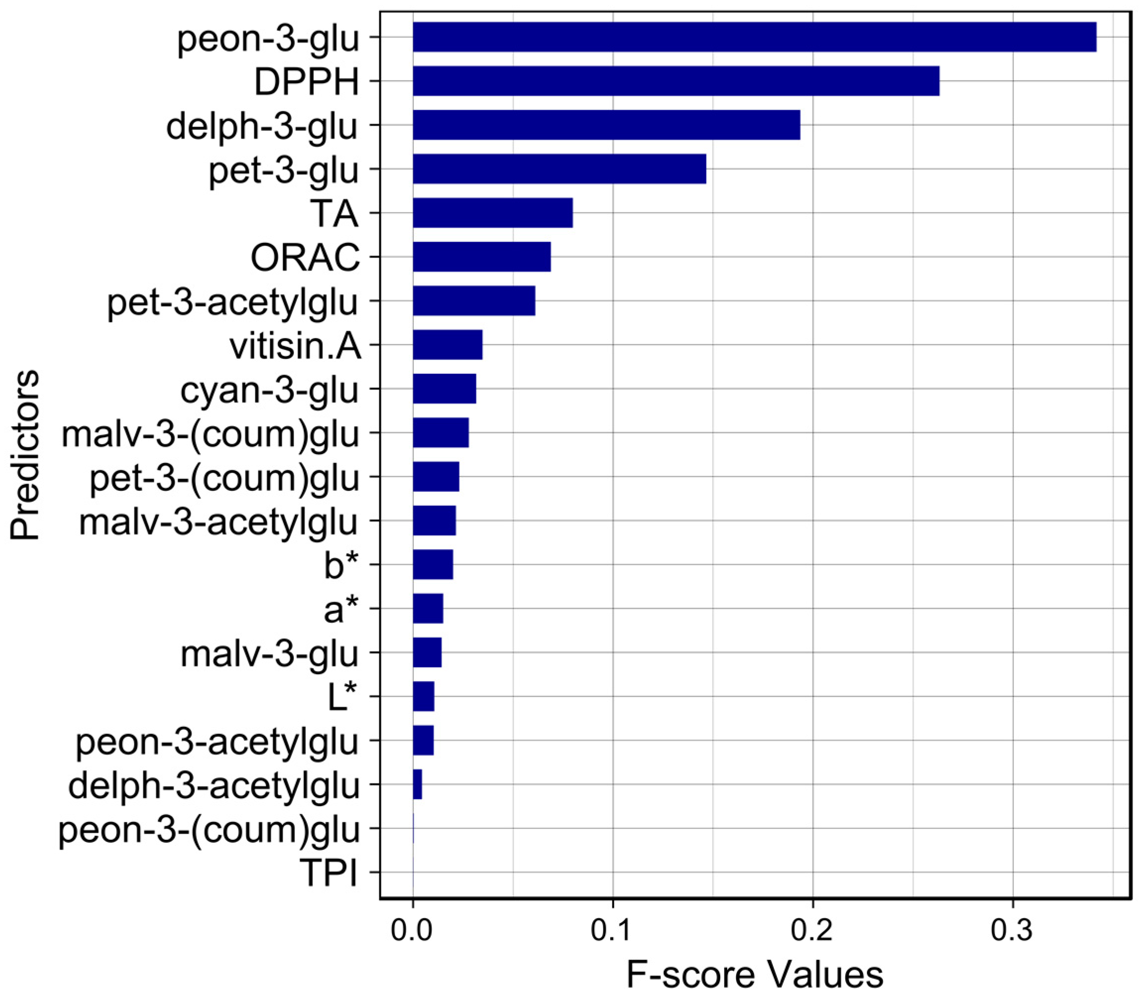
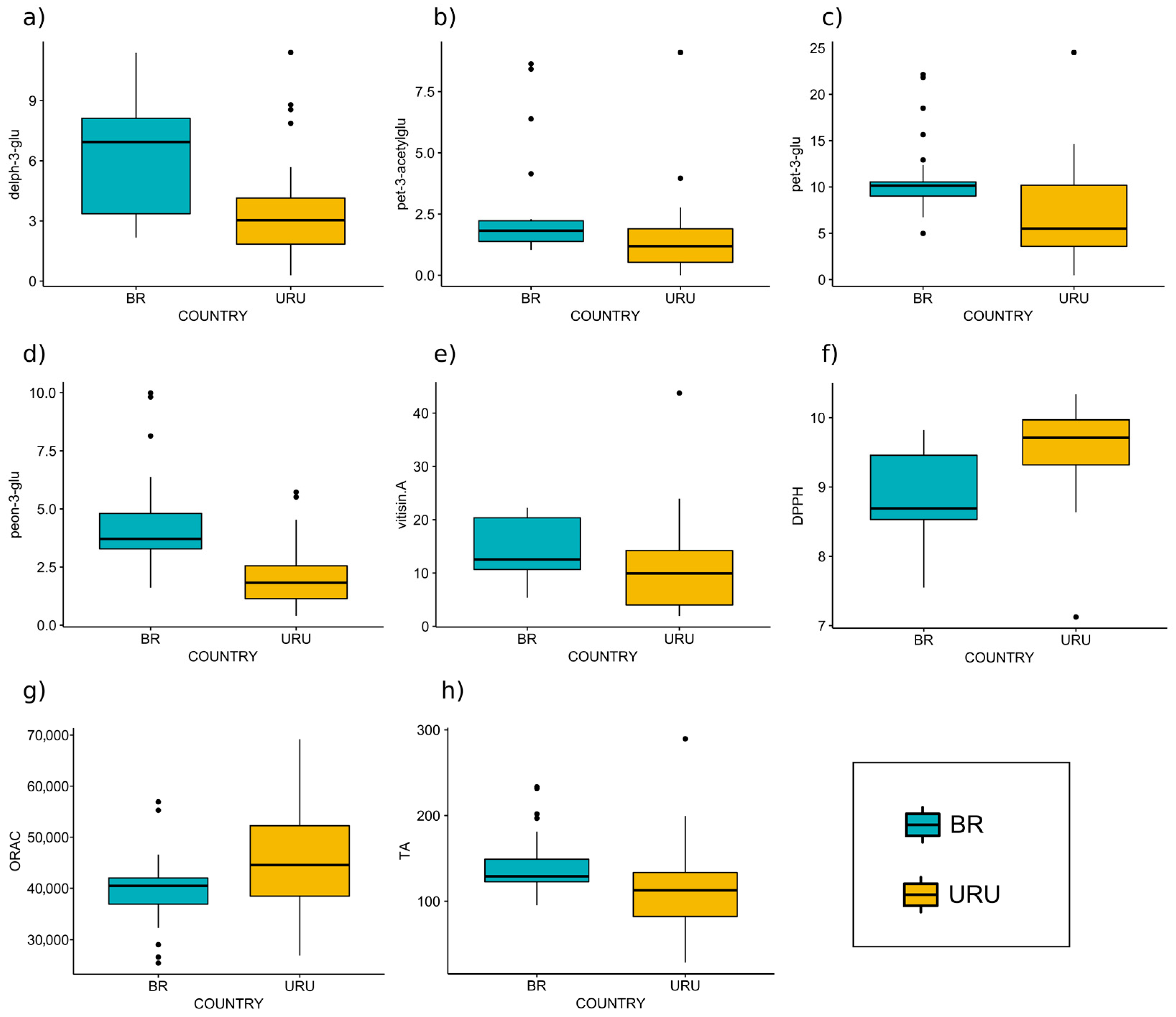
3.2. Analysis of Variable Importance

The group of anthocyanidin-3-glucosides comprises the main group of anthocyanins in wine, with malvidin-3-glucoside usually being the main component. In our study, three out of the five individual anthocyanins that were influential with regard to the classification of Tannat wines′ (peon-3-glu, delph-3-glu, and pet-3-glu) are part of this group. In spite of being in the majority, malv-3-glu is not one of the main variables responsible for the classification. Gutiérrez et al. found that malv-3-glu did not differentiate Chilean Merlot, Carménère, and Cabernet Sauvignon wines that were produced in different valleys [46]. On the other hand, they found that malv-3-(coum)glu played an important role, together with other anthocyanins, in this differentiation. In a previous study of the Cabernet Sauvignon classification according to geographical origin (Brazil and Chile), we found that L *, DPPH, delph-3-acetylglu, peon-3-(coum)glu, and pet-3-acetylglu were relevant variables for the classification [25].

Tannat wines have lower methyl–transferase activity compared to other wine varieties [7]. This allows the accumulation of delphinidins and petunidins, making these anthocyanins especially important in Tannat. This could explain, at least in part, the important role of delph-3-glu and pet-3-glu in Tannat wine classification. Another possible contribution pertains to the percentage of primitive anthocyanins (delph-3-glu and pet-3-glu), which may provide a significant indicator of the weather conditions pertaining to the ripening of grapes [47]. Therefore, these two anthocyanins could contribute to wine classification due to climatic differences in different wine production regions, which possibly affect the ripening process.

We then separately analyzed the most discriminating parameters according to the country of origin. Figure 4 presents the boxplot for each compound, stratified according to the country or origin. We note that most of the parameter values overlap. Most of the anthocyanin concentrations (including TA) are lower for the Uruguayan samples, while the DPPH and ORAC values of these samples are slightly higher, indicating that the anthocyanins are not the most relevant contributors to antioxidant activity.

4. Conclusions

In this study, we applied data mining techniques to classify Brazilian and Uruguayan Tannat wine samples. To our knowledge, this paper is the first to classify Tannat wines using SVM and to identify the variables that contributed most significantly to the classification. Using the original imbalanced dataset (28 Uruguayan samples and 9 Brazilian samples), the classification model achieved an accuracy rate of 72.97% and an MCC of 0.45. This performance improved when we added new synthetic Brazilian samples to the dataset. The best overall accuracy (94.64) and MCC (0.90) occurred when at least two, six, or eight variables were used, including, in the following order: peon-3-glu, DPPH, delph-3-glu, pet-3-glu, TA, ORAC, pet-3-acetylglu, and vitisin A. This finding proves that these variables are the most relevant for differentiating Tannat wine samples with respect to their geographical origin, and that the addition of synthetic samples can improve the classification model.

The identification of the most important parameters is useful for reducing time and resources put forth when classifying future wines. Additionally, understanding the behavior of wine chemical components is also important, as that knowledge serves as an information source for companies to preserve, maintain, and ensure the quality of wine, and to avoid fraud. Furthermore, the soil, climatic conditions, type of harvest, and conditions for production contribute to the characteristics that make a unique wine from a particular region, which explains the difference found among the parameter concentrations for each respective country in this study. The use of SVM allowed researchers to discriminate between the regions, whereas the PCA score plot only shows the overlapping of samples for each class. Therefore, this methodology can be applied for certification purposes that, in general, involved the origin of other wines and food products.

References

1. Gómez-Meire, S.; Campos, C.; Falqué, E.; Díaz, F.; Fdez-Riverola, F. Assuring the authenticity of northwest Spain white wine varieties using machine learning techniques. Food Res. Int. 2014, 60, 230–240. [Google Scholar] [CrossRef]
2. Luykx, D.M.A.M.; van Ruth, S.M. An overview of analytical methods for determining the geographical origin of food products. Food Chem. 2008, 107, 897–911. [Google Scholar] [CrossRef]
3. Geana, E.I.; Popescu, R.; Costinel, D.; Dinca, O.R.; Stefanescu, I.; Ionete, R.E.; Bala, C. Verifying the red wines adulteration through isotopic and chromatographic investigations coupled with multivariate statistic interpretation of the data. Food Control 2016, 62, 1–9. [Google Scholar] [CrossRef]
4. Versari, A.; Laurie, V.F.; Ricci, A.; Laghi, L.; Parpinello, G.P. Progress in authentication, typification and traceability of grapes and wines by chemometric approaches. Food Res. Int. 2014, 60, 2–18. [Google Scholar] [CrossRef]
5. Juan Gennari, A. A letter by the Regional Editor for South America: From varietals to terroir. Wine Econ. Policy 2014, 3, 69–70. [Google Scholar] [CrossRef]
6. González-Neves, G.; Gil, G.; Barreiro, L.; Favre, G. Pigment profile of red wines cv. Tannat made with alternative winemaking techniques. J. Food Compos. Anal. 2010, 23, 447–454. [Google Scholar] [CrossRef]
7. González-Neves, G.; Franco, J.; Barreiro, L.; Gil, G.; Moutounet, M.; Carbonneau, A. Varietal differentiation of Tannat, Cabernet-Sauvignon and Merlot grapes and wines according to their anthocyanic composition. Eur. Food Res. Technol. 2007, 225, 111–117. [Google Scholar] [CrossRef]
8. Welke, J.E.; Manfroi, V.; Zanus, M.; Lazzarotto, M.; Zini, C.A. Differentiation of wines according to grape variety using multivariate analysis of comprehensive two-dimensional gas chromatography with time-of-flight mass spectrometric detection data. Food Chem. 2013, 141, 3897–3905. [Google Scholar] [CrossRef] [PubMed]
9. Xiao, Z.; Liu, S.; Gu, Y.; Xu, N.; Shang, Y.; Zhu, J. Discrimination of cherry wines based on their sensory properties and aromatic fingerprinting using HS-SPME-GC-MS and multivariate analysis. J. Food Sci. 2014, 79, C284–C294. [Google Scholar] [CrossRef] [PubMed]
10. Rešetar, D.; Marchetti-Deschmann, M.; Allmaier, G.; Katalinić, J.P.; Pavelić, S.K. Matrix assisted laser desorption ionization mass spectrometry linear time-of-flight method for white wine fingerprinting and classification. Food Control 2016, 64, 157–164. [Google Scholar] [CrossRef]
11. Płotka-Wasylka, J.; Simeonov, V.; Morrison, C.; Namieśnik, J. Impact of selected parameters of the fermentation process of wine and wine itself on the biogenic amines content: Evaluation by application of chemometric tools. Microchem. J. 2018, 142, 187–194. [Google Scholar] [CrossRef]
12. Bonello, F.; Cravero, M.; Dell’Oro, V.; Tsolakis, C.; Ciambotti, A. Wine Traceability Using Chemical Analysis, Isotopic Parameters, and Sensory Profiles. Beverages 2018, 4, 54. [Google Scholar] [CrossRef]
13. Aceto, M.; Bonello, F.; Musso, D.; Tsolakis, C.; Cassino, C.; Osella, D. Wine Traceability with Rare Earth Elements. Beverages 2018, 4, 23. [Google Scholar] [CrossRef]
14. Zielinski, A.A.F.; Haminiuk, C.W.I.; Nunes, C.A.; Schnitzler, E.; Ruth, S.M.; Granato, D. Chemical composition, sensory properties, provenance, and bioactivity of fruit juices as assessed by chemometrics: A critical review and guideline. Compre. Rev. Food Sci. food Saf. 2014, 13, 300–316. [Google Scholar] [CrossRef]
15. Callao, M.P.; Ruisánchez, I. An overview of multivariate qualitative methods for food fraud detection. Food Control 2018, 86, 283–293. [Google Scholar] [CrossRef]
16. Condurso, C.; Cincotta, F.; Tripodi, G.; Verzera, A. Characterization and ageing monitoring of Marsala dessert wines by a rapid FTIR-ATR method coupled with multivariate analysis. Eur. Food Res. Technol. 2018, 244, 1073–1081. [Google Scholar] [CrossRef]
17. Ríos-Reina, R.; García-González, D.L.; Callejón, R.M.; Amigo, J.M. NIR spectroscopy and chemometrics for the typification of Spanish wine vinegars with a protected designation of origin. Food Control 2018, 89, 108–116. [Google Scholar] [CrossRef]
18. Ioannou-Papayianni, E.; Kokkinofta, R.I.; Theocharis, C.R. Authenticity of Cypriot sweet wine commandaria using FT-IR and chemometrics. J. Food Sci. 2011, 76, C420–C427. [Google Scholar] [CrossRef] [PubMed]
19. Ropodi, A.I.; Panagou, E.Z.; Nychas, G.-J. Data mining derived from food analyses using non-invasive/non-destructive analytical techniques; determination of food authenticity, quality & safety in tandem with computer science disciplines. Trends Food Sci. Technol. 2016, 50, 11–25. [Google Scholar] [CrossRef]
20. Guo, H.; Li, Y.; Jennifer, S.; Gu, M.; Huang, Y.; Gong, B. Learning from class-imbalanced data: Review of methods and applications. Expert Syst. Appl. 2017, 73, 220–239. [Google Scholar] [CrossRef]
21. Majchrzak, T.; Wojnowski, W.; Płotka-Wasylka, J. Classification of Polish wines by application of ultra-fast gas chromatography. Eur. Food Res. Technol. 2018, 1–9. [Google Scholar] [CrossRef]
22. Capron, X.; Massart, D.L.; Smeyers-Verbeke, J. Multivariate authentication of the geographical origin of wines: A kernel SVM approach. Eur. Food Res. Technol. 2007, 225, 559–568. [Google Scholar] [CrossRef]
23. Ríos-Reina, R.; Elcoroaristizabal, S.; Ocaña-González, J.A.; García-González, D.L.; Amigo, J.M.; Callejón, R.M. Characterization and authentication of Spanish PDO wine vinegars using multidimensional fluorescence and chemometrics. Food Chem. 2017, 230, 108–116. [Google Scholar] [CrossRef] [PubMed]
24. Jurado, J.M.; Alcázar, Á.; Palacios-Morillo, A.; De Pablos, F. Classification of Spanish DO white wines according to their elemental profile by means of support vector machines. Food Chem. 2012, 135, 898–903. [Google Scholar] [CrossRef] [PubMed]
25. da Costa, N.L.; Castro, I.A.; Barbosa, R. Classification of Cabernet Sauvignon from Two Different Countries in South America by Chemical Compounds and Support Vector Machines. Appl. Artif. Intell. 2016, 30, 679–689. [Google Scholar] [CrossRef]
26. Soares, F.; Anzanello, M.J.; Fogliatto, F.S.; Marcelo, M.C.A.; Ferrão, M.F.; Manfroi, V.; Pozebon, D. Element selection and concentration analysis for classifying South America wine samples according to the country of origin. Comput. Electron. Agric. 2018, 150, 33–40. [Google Scholar] [CrossRef]
27. Singleton, V.L.; Rossi, J.A. Colorimetry of total phenolics with phosphomolybdic-phosphotungstic acid reagents. Am. J. Enol. Vitic. 1965, 16, 144–158. [Google Scholar]
28. Fuleki, T.; Francis, F.J. Determination of total anthocyanin and degradation index for cranberry juice. Food Sci. 1968, 33, 78–83. [Google Scholar] [CrossRef]
29. Boido, E.; Alcalde-Eon, C.; Carrau, F.; Dellacassa, E.; Rivas-Gonzalo, J.C. Aging effect on the pigment composition and color of Vitis vinifera L. cv. Tannat wines. Contribution of the main pigment families to wine color. J. Agric. Food Chem. 2006, 54, 6692–6704. [Google Scholar] [CrossRef] [PubMed]
30. Arnous, A.; Makris, D.P.; Kefalas, P. Effect of principal polyphenolic components in relation to antioxidant characteristics of aged red wines. J. Agric. Food Chem. 2001, 49, 5736–5742. [Google Scholar] [CrossRef] [PubMed]
31. Huang, D.; Ou, B.; Hampsch-Woodill, M.; Flanagan, J.A.; Prior, R.L. High-throughput assay of oxygen radical absorbance capacity (ORAC) using a multichannel liquid handling system coupled with a microplate fluorescence reader in 96-well format. J. Agric. Food Chem. 2002, 50, 4437–4444. [Google Scholar] [CrossRef] [PubMed]
32. Witten, I.H.; Frank, E.; Hall, M.A. Data Mining: Practical Machine Learning Tools and Techniques; Elsevier: Amsterdam, The Netherlands, 2011. [Google Scholar]
33. Chawla, N.V.; Bowyer, K.W.; Hall, L.O.; Kegelmeyer, W.P. SMOTE: Synthetic minority over-sampling technique. J. Artif. Intell. Res. 2002, 16, 321–357. [Google Scholar] [CrossRef]
34. Team, the R.C. R: A language and environment for statistical computing. R Foundation for Statistical Computing. Available online: https://www.R-project.org/ (accessed on 30 November 2018).
35. Kuhn, M. The caret package. Available online: http://caret.r-forge.r-project.org/ (accessed on 30 November 2018).
36. Wickham, H. Ggplot2: Elegant Graphics for Data Analysis; Springer-Verlag New York: New York, NY, USA, 2009. [Google Scholar]
37. Cortes, C.; Vapnik, V. Support-vector networks. Mach. Learn. 1995, 20, 273–297. [Google Scholar] [CrossRef] [Green Version]
38. Xue, H.; Yang, Q.; Chen, S. SVM: Support vector machines. In The Top Ten Algorithms in Data Mining; Taylor & Francis Group: Abingdon-on-Thames, UK, 2009; pp. 37–59. [Google Scholar]
39. Noori, R.; Abdoli, M.A.; Ghasrodashti, A.A.; Jalili Ghazizade, M. Prediction of municipal solid waste generation with combination of support vector machine and principal component analysis: A case study of Mashhad. Environ. Prog. Sustain. Energy 2009, 28, 249–258. [Google Scholar] [CrossRef]
40. Chandrashekar, G.; Sahin, F. A survey on feature selection methods. Comput. Electr. Eng. 2014, 40, 16–28. [Google Scholar] [CrossRef]
41. Chen, Y.-W.; Lin, C.-J. Combining SVMs with various feature selection strategies. In Feature Extraction; Springer: Berlin, Germany, 2006; pp. 315–324. [Google Scholar]
42. Liu, F.; Guo, W.; Fouche, J.-P.; Wang, Y.; Wang, W.; Ding, J.; Zeng, L.; Qiu, C.; Gong, Q.; Zhang, W.; et al. Multivariate classification of social anxiety disorder using whole brain functional connectivity. Brain Struct. Funct. 2015, 220, 101–115. [Google Scholar] [CrossRef] [PubMed]
43. Turra, C.; de Lima, M.D.; Fernandes, E.A.D.N.; Bacchi, M.A.; Barbosa, F.; Barbosa, R. Multielement determination in orange juice by ICP-MS associated with data mining for the classification of organic samples. Inf. Process. Agric. 2017, 4, 199–205. [Google Scholar] [CrossRef]
44. Marin, G.; Dominio, F.; Zanuttigh, P. Hand gesture recognition with jointly calibrated leap motion and depth sensor. Multimed. Tools Appl. 2016, 75, 14991–15015. [Google Scholar] [CrossRef]
45. Adnane, M.; Belouchrani, A. Heartbeats classification using QRS and T waves autoregressive features and RR interval features. Expert Syst. 2017, 34, e12219. [Google Scholar] [CrossRef]
46. Gutiérrez, L.; Quintana, F.A.; Baer, D.; von Mardones, C. Multivariate Bayesian discrimination for varietal authentication of Chilean red wine. J. Appl. 2011, 4763, 1–28. [Google Scholar] [CrossRef]
47. Río Segade, S.; Orriols, I.; Gerbi, V.; Rolle, L. Phenolic characterization of thirteen red grape cultivars from galicia by anthocyanin profile and flavanol composition. J. Int. Sci. Vigne Vin 2009, 43, 189–198. [Google Scholar] [CrossRef]
Figure 1. Schematic view of the Tannat wines analysis.
Beverages 04 00097 g001
Figure 2. Visual separation of wines based on PC1 (principal component) and PC2. (a) The original data; (b) the synthetic data added to the original data.
Beverages 04 00097 g002
Figure 3. F-score ranking of importance.
Beverages 04 00097 g003
Figure 4. Boxplots of the eight compounds selected by the F-score, along with SVM classification. (a) delph-3-glu variable; (b) pet-3-acetylglu variable; (c) pet-3-glu variable; (d) peon-3-glu; (e) vitisin A variable; (f) free radical scavenging capacity (DPPH) variable; (g) oxygen radical absorbance capacity (ORAC) variable; and (h) total anthocyanins (TA) variable.
Beverages 04 00097 g004