Wineinformatics: Using the Full Power of the Computational Wine Wheel to Understand 21st Century Bordeaux Wines from the Reviews

Abstract

Although wine has been produced for several thousands of years, the ancient beverage has remained popular and even more affordable in modern times. Among all wine making regions, Bordeaux, France is probably one of the most prestigious wine areas in history. Since hundreds of wines are produced from Bordeaux each year, humans are not likely to be able to examine all wines across multiple vintages to define the characteristics of outstanding 21st century Bordeaux wines. Wineinformatics is a newly proposed data science research with an application domain in wine to process a large amount of wine data through the computer. The goal of this paper is to build a high-quality computational model on wine reviews processed by the full power of the Computational Wine Wheel to understand 21st century Bordeaux wines. On top of 985 binary-attributes generated from the Computational Wine Wheel in our previous research, we try to add additional attributes by utilizing a CATEGORY and SUBCATEGORY for an additional 14 and 34 continuous-attributes to be included in the All Bordeaux (14,349 wine) and the 1855 Bordeaux datasets (1359 wines). We believe successfully merging the original binary-attributes and the new continuous-attributes can provide more insights for Naïve Bayes and Supported Vector Machine (SVM) to build the model for a wine grade category prediction. The experimental results suggest that, for the All Bordeaux dataset, with the additional 14 attributes retrieved from CATEGORY, the Naïve Bayes classification algorithm was able to outperform the existing research results by increasing accuracy by 2.15%, precision by 8.72%, and the F-score by 1.48%. For the 1855 Bordeaux dataset, with the additional attributes retrieved from the CATEGORY and SUBCATEGORY, the SVM classification algorithm was able to outperform the existing research results by increasing accuracy by 5%, precision by 2.85%, recall by 5.56%, and the F-score by 4.07%. The improvements demonstrated in the research show that attributes retrieved from the CATEGORY and SUBCATEGORY has the power to provide more information to classifiers for superior model generation. The model build in this research can better distinguish outstanding and class 21st century Bordeaux wines. This paper provides new directions in Wineinformatics for technical research in data science, such as regression, multi-target, classification and domain specific research, including wine region terroir analysis, wine quality prediction, and weather impact examination.

1. Introduction

Science has its origins in attempts to understand the world in an empirically verified manner. To understand the world, one relies on testing it. In order to test ideas, you often need data. Each data point is a discrete record or a property of events that occurred in the world. Now, with the rise of the Internet, data has become abundant. What has also allowed for the rise of data science is the advancement in the application of statistically-based algorithms to make sense of these larger quantities of data. Within this emerging field, there are several different types of learning algorithms that provide utility. Specifically, there are four major types of learning algorithms based on the problem, the input/output, and methods (Supervised Learning [1], Unsupervised Learning [2], Semi-supervised Learning [3], and Reinforced Learning [4]). All of these methods are useful for discovering interesting information from large amounts of data within specific application domains.

Wine has been produced for several thousands of years. This ancient beverage has remained popular and even more affordable in modern times. According to the International Organization of Vine and Wine (OIV), who is the world’s authority on wine statistics, in 2018, 293 million hectoliters of wine were produced across 36 countries. This constitutes a 17% increase in wine production from 2017 to 2018 [5]. An endless number of varieties and flavors are provided to consumers, most of whom are not wine experts. Therefore, wine reviews and rankings produced by the experts, such as Robert Parker [6], and James Suckling [7], and wine review magazines, such as Wine Spectator [8], Wine Enthusiast [9], and Decanter [10], are important since they become part of the heuristics that drive consumers’ decision-making. Not only wine consumers can benefit from the wine reviews, but wine makers can also gain valuable information and knowledge from the expert reviews by knowing what factors contribute the most to quality, as determined by rankings. How to analyze and mine the large amount of available wine reviews is a major task to discover useful information for wine producers, distributors, and consumers. For example, Wine Spectator and Wine Advocator by Robert Parker have more than 385,000 and 450,000 reviews available, respectively.

Wineinformatics [11,12] incorporates data science and wine-related datasets, including physicochemical laboratory data and wine reviews, to discover useful information for wine producers, distributors, and consumers. Physicochemical laboratory data usually relates to the physicochemical composition analysis [13], such as acidity, residual sugar, alcohol, etc., to characterize wine. Physicochemical information is more useful for the wine-making process. However, physicochemical analysis cannot express the sensory quality of wine. Wine reviews are produced by sommeliers, who are people who specialize in wine. These wine reviews usually include aroma, flavors, tannins, weight, finish, appearance, and the interactions related to these wine sensations [14]. From a computer perspective, the physicochemical laboratory data is easy to read and apply analytics to. However, wine reviews’ data involves natural language processing and a degree of human bias. Therefore, in our previous research [15,16], a new technique named the Computational Wine Wheel was developed to accurately capture keywords, including not only flavors but also non-flavor notes, which always appear in the wine reviews.

The Bordeaux wine-making process started in the mid-1st century and became popular in England in the 12th century [17,18]. Today, Bordeaux is the biggest wine delivering district in France and one of the most influential wine districts in the world. Many data mining efforts [19,20,21] focused on searching the relationship between the price and vintage of Bordeaux wines from historical and economic data. Shanmuganathan et al. applied decision tree and statistical methods for modeling seasonal climate effects on grapevine yield and wine quality [22]. Noy et al. developed the ontology on Bordeaux wine [23,24]. Most of these Bordeaux or wine-related data mining research applied their work on small-to-medium-sized wine datasets [25,26,27,28]. However, as stated in the beginning of the introduction, with the rise of the Internet, data has become abundant, including wine-related data. The amount of data is no longer analyzable by humans. Therefore, in our previous Wineinformatics research [29], we explored all 21st century Bordeaux wines by creating a publicly available dataset with 14,349 Bordeaux wines [30]. To the best of our knowledge, this dataset is the largest wine-region specific dataset in the open literature. Based on the official Bordeaux wine classification in 1855 [31], we generated an 1855 Bordeaux Wine Official Classification Dataset to investigate the elite wines. This dataset is a subset of all 21st century Bordeaux wines and contains 1359 wines.

The goal of this paper is to improve from our previous research [29] by incorporating the full power of the Computational Wine Wheel to gain more insights in 21st century Bordeaux wines. More specifically, instead of only using “specific words” to map wine reviews and assign “normalized” binary (0/1) attributes to the wine in all previous Wineinformatics research, we want to include “category” and “subcategory” into the natural language processing component and assign corresponding continuous-attributes. For example, apple and peach will be under “tree fruit” in the subcategory column and “fruity” in the category column. In previous Wineinformatics research, a wine review with peach and apple would be converted into a positive (1) in peach, a positive (1) in apple, and negative (0) in all other attributes. However, in this research, the same wine review will be converted into the “fruity” category with an accumulated value of 2, the “tree fruit” subcategory with an accumulated value of 2, plus all the binary attributes that appeared previously. We are interested in how the word frequency in the categories and subcategories would affect the machine learning process to understand Bordeaux wines. We believe, by successfully merging the original binary-attributes and the new continuous-attributes, can provide more insights for Naïve Bayes and Support Vector Machine (SVM) to build the model for a wine grade category prediction.

2. Materials and Methods

Data science is the study of data with an application domain. The source, the pre-processing, and the creation of the data are all major factors for the quality of the data. Since the data in this research is about wine reviews, which is stored in a human language format, Natural Language Processing (NLP) is needed [32].

2.1. Wine Spectator

Many research efforts indicate that wine judges may demonstrate intra- and inter-inconsistencies while tasting designated wines [33,34,35,36,37,38,39,40]. The Wine Spectator is a wine magazine company that provides consistent creditable wine reviews periodically by a group of wine region specific reviewers. The company has published approximately 385,000 wine reviews. The magazine publishes 15 issues a year, and there are between 400 and 1000 wine reviews per issue. In our previous Wineinformatics research [11,12], more than 100,000 wine reviews were gathered and analyzed across all wine regions. This dataset was used to test wine reviewers’ accuracy in predicting a wine’s credit score. Wine Spectator reviewers received more than 87% accuracy when evaluated with the SVM method while predicting whether a wine received a credit score higher than 90/100 points [11]. The regression analysis on predicting a wine’s actual score based on the reviews also has an outstanding result with only a 1.6 average score difference on a Mean Absolute Error (MAE) evaluation [12]. These results support Wine Spectator’s prestigious standing in the wine industry. 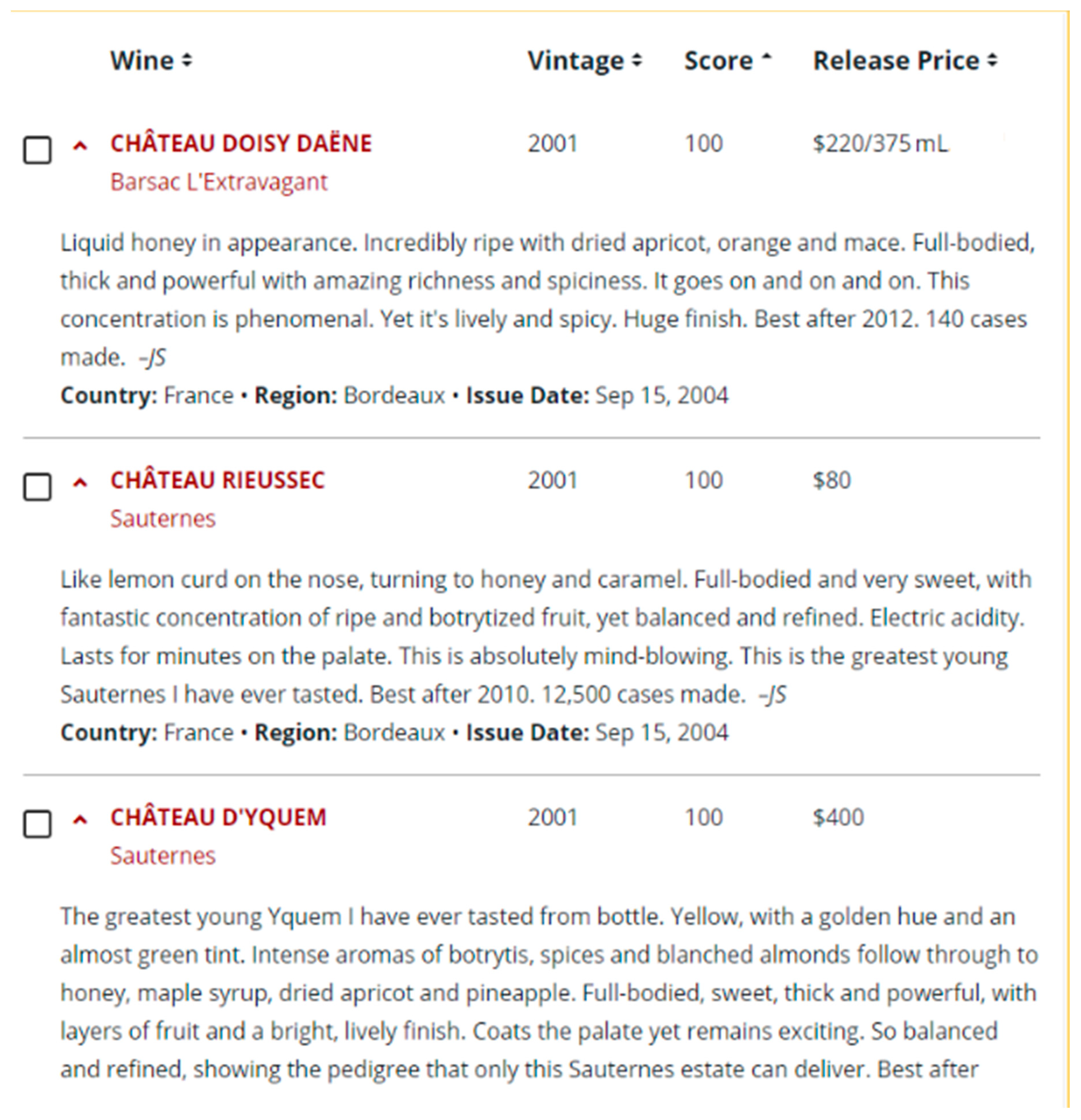Figure 1 is the example of wine reviews on WineSpectator.com.

There is a 50–100 score scale on evaluating the wine used by Wine Spectator. Details of the score scale can be described as:

• 95–100 Classic: a great wine
• 90–94 Outstanding: a wine of superior character and style
• 85–89 Very good: a wine with special qualities
• 80–84 Good: a solid, well-made wine
• 75–79 Mediocre: a drinkable wine that may have minor flaws
• 50–74 Not recommended

2.2. Bordeaux Datasets

In our previous research [29], we explored all 21st century Bordeaux wines by creating a publicly available dataset with 14,349 Bordeaux wines [30]. In addition, based on the official Bordeaux wine classification in 1855 [31], we generated an 1855 Bordeaux Wine Official Classification Dataset to investigate the elite wines. This dataset is a subset of all 21st century Bordeaux wines and contains 1359 wines. All of the wine reviews in the datasets came from Wine Spectator in a human language format. We processed the reviews through the Computational Wine Wheel, which works as a dictionary using one-hot encoding to convert words into vectors. For example, in a wine review, there are some words that contain fruits such as apple, blueberry, plum, etc. If the word matches the attribute in the computation wine wheel, it will be 1. Otherwise, it will be 0. The Computational Wine Wheel is also equipped with a generalization function to map similar words into the same coding. For example, fresh apple, apple, and ripe apple are generalized into “apple” since they represent the same flavor. Yet, green apple belongs to a “green apple” since the flavor of green apple is different from apple. The score of the wine is also attached to the data as the last attribute, also known as the label. For supervised learning, in order to understand the characteristics of classic (95+) and outstanding (90–94) wines, we use 90 points as a cutoff value. If a wine receives a score equal/above 90 points out of 100, we mark the label as a positive (+) class to the wine. Otherwise, the label would be a negative (−) class. There are some wines that received a ranged score, such as 85–88. We use the average of the ranged score to decide and assign the label. Some detailed score-distribution and number-of-wine-reviewed-each-year statistics are available in Reference [29].

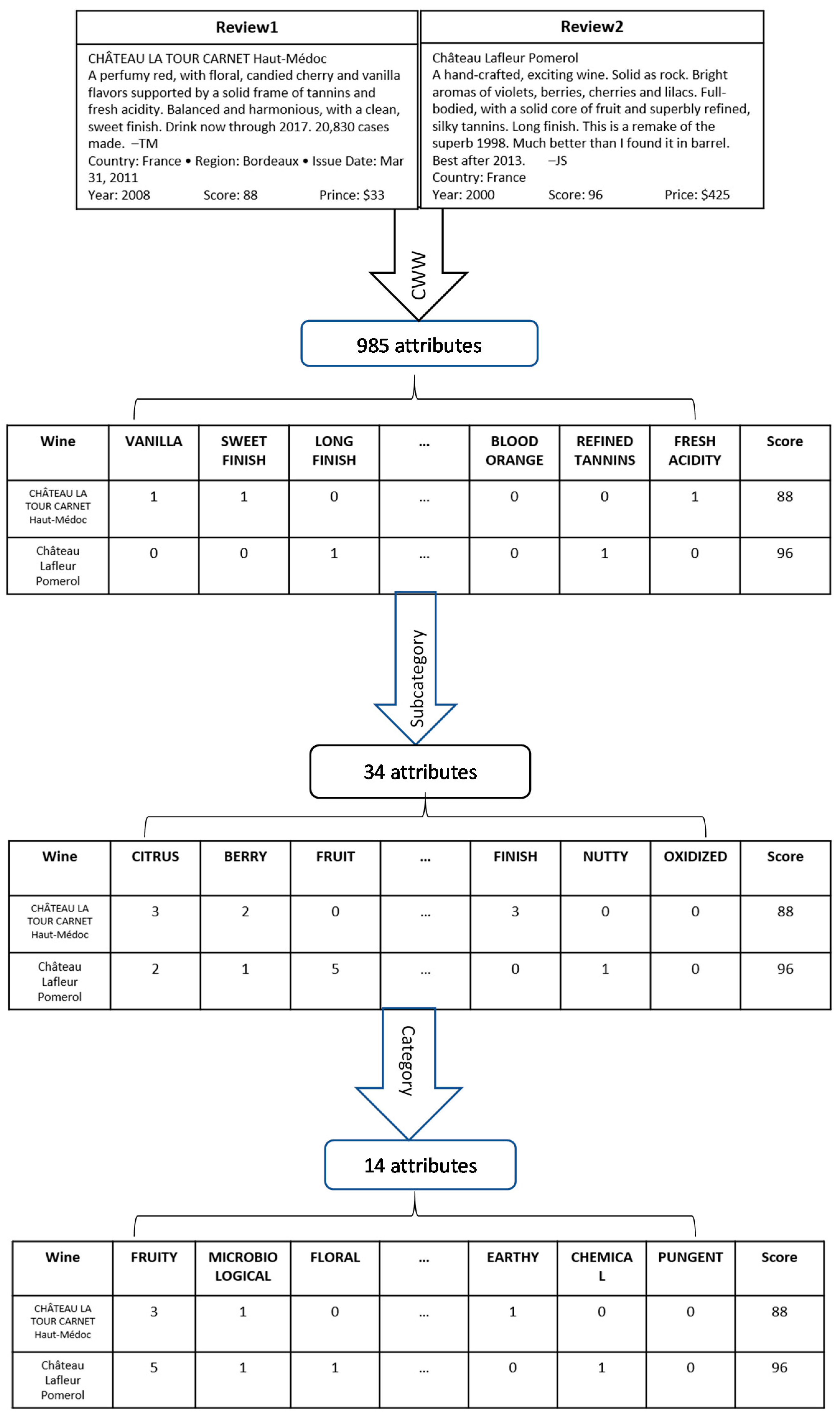
In this paper, we want to use the full power of the Computational Wine Wheel to extract more information from the same Bordeaux datasets. In the latest version of the Computational Wine Wheel, there are four columns CATEGORY_NAME, SUBCATEGORY_NAME, SPECIFIC_NAME, and NORMALIZED_NAME. There are 14 attributes in the CATEGORY_NAME, 34 in the SUBCATEGORY_NAME, 1881 in the SPECIFIC_NAME, and 985 in the NORMALIZED_NAME. The details can be found in

Table 1. Summary of all wine attributes.

CATEGORY_NAME	SUBCATEGORY_NAME	SPECIFIC_NAME	NORMALIZED_NAME
CARAMEL	CARAMEL	71	40
CHEMICAL	PETROLEUM	9	5
	SULFUR	11	10
	PUNGENT	4	3
EARTHY	EARTHY	72	31
	MOLDY	2	2
FLORAL	FLORAL	61	39
FRUITY	BERRY	49	28
	CITRUS	37	23
	DRIED FRUIT	67	60
	FRUIT	22	9
	OTHER	25	18
	TREE FRUIT	39	31
	TROPICAL FRUIT	48	27
FRESH	FRESH	41	29
	DRIED	25	21
	CANNED/COOKED	16	15
MEAT	MEAT	25	13
MICROBIOLOGICAL	YEASTY	5	4
	LACTIC	14	6
NUTTY	NUTTY	25	15
OVERALL	TANNINS	90	4
	BODY	50	23
	STRUCTURE	40	2
	ACIDITY	40	3
	FINISH	184	5
	FLAVOR/DESCRIPTORS	649	432
OXIDIZED	OXIDIZED	1	1
PUNGENT	HOT	3	2
	COLD	1	1
SPICY	SPICE	83	44
WOODY	RESINOUS	24	9
	PHENOLIC	6	4
	BURNED	47	26

. Contrary to the previous data, which used only a SPECIFIC_NAME to match wine reviews and NORMALIZED_NAME to encode wine attributes, this research includes two more columns of the Computational Wine Wheel, SPECIFIC_NAME and NORMALIZED_NAME. For example, for a wine with “fresh apple” and “crushed cherry” in the review, the computational wine wheel will encode a 1 for the “apple” attribute since apple is the normalized attribute for “fresh apple” and a 1 for the “cherry” attribute since cherry is the normalized attribute for “crushed cherry.” In this research, not only “apple” and “cherry” attributes will be 1, the new data will count “tree fruit” twice and “fruity” twice since both apple and cherry are under the “tree fruit” SUBCATEGORY_NAME and “fruity” CATEGORY_NAME columns. The new dataset changes from a purely binary dataset to a mixed data format dataset.

The flowchart presented in Figure 2 shows the process of converting reviews into a machine readable format. Reviews are processed using the computational wine wheel into NORMALIZED_NAME, SUBCATEGORY_NAME, and CATEGORY_NAME.

After preprocessing, 14 category and 34 subcategory attributes were added into both datasets, creating a total of 1033 attributes. However, the attributes in SUBCATEGORY_NAME and CATEGORY_NAME are continuous instead of binary values, and the ranges of each attribute are variable. The learning algorithm will give one feature more weight than the other if we do not perform normalization with our attributes, especially when the attributes in NORMALIZED_NAME are binary. Normalization can help speed up the learning process as well as avoid numerical problems, such as loss of accuracy due to arithmetic overflow [41]. In this research, we used Min-Max normalization (Equation (1)) to scale the attribute values to 0–1. The formula is as follows.

$$x^{\prime } =\frac{x-\min (x)}{\max (x)-\min (x)}$$

(1)

where $x$ is an original value,$x^{\prime }$ is the normalized value,$\min (x)$ is the minimum value among all x, and$\max (x)$ is the maximum value among all x.

2.3. Supervised Learning Algorithms and Evaluations

Supervised learning builds a model through labeled datasets to make predictions. If the label is a continuous variable, it is known as regression. If the label is a discrete variable, it is known as classification. In this research, we are trying to understand what makes an outstanding 21st century Bordeaux wine. More specifically, what are the characteristics of classic (95+) and outstanding (90–94) Bordeaux. In order to achieve this goal, 90 points were chosen as the cutoff value. If a wine receives a score equal/above 90 points out of 100, we mark the label as a positive (+) class for the wine. Otherwise, the label would be a negative (−) class. Therefore, the task we are doing is classifying supervised learning. The evaluation metrics (accuracy, precision, recall, and F-score) were used to evaluate the performance of models with five-fold cross-validation. In this research, we applied Naïve Bayes and SVM as our classification algorithms to build the model of 21st century Bordeaux wines. If the model can accurately predict a wine’s grade category through the review, it means the model can capture the essence of high-quality wines.

2.3.1. Naïve Bayes Classifier

Throughout Wineinformatics research, the Naïve Bayes classifier has been considered the most suitable white-box classification algorithm. A Naïve Bayes classifier is a simple probabilistic classifier that applies Bayes’ Theorem with two assumptions: (1) there is no dependence between attributes. For example, the word APPLE appearing in a review has nothing to do with the appearance of the word FRUITY even though both words might appear in the same review. (2) In terms of the importance of the label/outcome, each attribute is treated the same. For example, the word APPLE and the word FRUITY have equal importance in influencing the prediction of wine quality. The assumptions made by Naïve Bayes are often incorrect in real-world applications. As a matter of fact, the assumption of independence between attributes is always wrong, but Bayes still often works well in practice [42,43].

Here is the Bayes’ Theorem:

$$P(Y|X)=\frac{P(X|Y)P\left(Y\right)}{P\left(X\right)}$$

(2)

where $P(X|Y)$ is the posterior probability of Y belonging to a particular class when X happens, P(Y) is the prior probability of Y, and P(X) is the prior probability of X.

Based on the Bayes’ Theorem, the Naïve Bayes classifier is defined as:

$$P\left(Y|X_1,X_2,\dots ,X_n\right)=\frac{P\left(X_1,X_2,\dots ,X_n|Y\right)P\left(Y\right)}{P\left(X_1,X_2,\dots ,X_n\right)}=\frac{P\left(X_1|Y\right)P\left(X_2|Y\right)\dots P\left(X_n|Y\right)P\left(Y\right)}{P\left(X_1,X_2,\dots ,X_n\right)}$$

(3)

Equation (3) computes all posterior probabilities of all values in X for all values in Y. For a traditional bi-class classification problem in terms of positive and negative cases, the Naïve Bayes classifier calculates a posterior probability for the positive case and a posterior probability for the negative case. The case with the higher posterior probability is the prediction made by the Naïve Bayes classifier. There are two main Naïve Bayes classifiers based on the type of attributes: Gaussian Naïve Bayes classifier [44] for continuous attributes, and Bernoulli Naïve Bayes classifier [45] for binary attributes.

In the Gaussian Naïve Bayes classifier (Equation (4)) [44], it is assumed that the continuous values associated with each attribute are distributed according to a Gaussian distribution. A Gaussian distribution is also known as a normal distribution.

$$P(X_i|Y)=\frac{1}{6_y\sqrt{2\mathsf{\pi }}}\exp (-\frac{{(X_i-{\mu }_y)}^2}{2\mathsf{\pi }{6}_y{}^2})$$

(4)

where ${\mu }_y$ is the sample mean, and $6_y$ is the sample standard deviation.

In the Bernoulli Naïve Bayes classifier (Equation (5)) [45], the attributes are binary variables. The frequency of a word in the reviews is used as the probability.

$$P(X_i|Y)=\frac{N_{ic}}{N_C}$$

(5)

where $N_{ic}$ is the number of samples/reviews having attribute $X_i$ and belonging to class $Y$, and $N_C$ is the number of samples/reviews belonging to class $Y$.

When a value of X never appears in the training set, the prior probability of that value of X will be 0. If we do not use any techniques, $P\left(Y|X_{1,}{X}_2,\dots X_n\right)$ will be 0, even when some of the other prior probabilities of X are significant. This case does not seem fair to other X. Therefore, we use Laplace smoothing (Equation (6)) [45] to handle zero prior probability by modifying Equation (5) slightly.

Laplace Smoothing:

$$P(X_i|Y)=\frac{N_{ic}+1}{N_C+c}$$

(6)

where c is the number of values in Y.

In our dataset, as mentioned in Section 2, 985 attributes captured by NORMALIZED_NAME are binary values, while 14 and 34 attributes captured by SUBCATEGORY_NAME and CATEGORY_NAME are continuous values. To calculate the posterior probability in the Naïve Bayes classifier for a training dataset with both continuous and binary values, this research multiplies the posterior probability produced by Gaussian Naïve Bayes on continuous attributes with the posterior probability produced by Bernoulli Naïve Bayes with Laplace on binary attributes.

2.3.2. SVM

SVM are supervised learning models with associated learning algorithms that analyze data and recognize patterns used for classification and regression analysis [46]. Classification-based SVM builds a model by constructing “a hyperplane or set of hyperplanes in a high-dimensional or infinite-dimensional space, which can be used for classification, regression, or other tasks. Intuitively, a good separation is achieved by the hyperplane that has the largest distance to the nearest training data point of any class (so-called functional margin), since, in general, the larger the margin is, the lower the generalization error of the classifier is.” After constructing the model, testing data is used to predict its accuracy. SVM light [47] is the version of SVM that was used to perform the classification of attributes for this project.

2.4. Evaluation Methods

To evaluate the effectiveness of the classification model, several standard statistical evaluation metrics are used in this paper: True Positive (TP), True Negative (TN), False Positive (FP), and False Negative (FN). We have refined their definitions for our research as follows.

• TP: The real condition is true (1) and predicted as true (1); 90+ wine correctly classified as 90+ wine;
• TN: The real condition is false (−1) and predicted as false (−1); 89− wine correctly classified as 89− wine;
• FP: The real condition is false (−1) but predicted as true (1); 89− wine incorrectly classified as 90+ wine;
• FN: The real condition is true (1) but predicted as false (−1); 90+ wine incorrectly classified as 89− wine;

If we use 90 points as a cutoff value in this research, TP would be “if a wine scores equal/above 90 and the classification model also predicts it as equal/above 90.” Below are our evaluation metrics.

Accuracy (Equation (7)): The proportion of wines that have been correctly classified among all wines. Accuracy is a very intuitive metric.

$$\mathrm{Accuracy}=\frac{\mathrm{TP}+\mathrm{TN}}{\mathrm{TP}+\mathrm{TN}+\mathrm{FP}+\mathrm{FN}}$$

(7)

Recall (Equation (8)): The proportion of 90+ wines that were identified correctly. Recall explains the sensitivity of the model to 90+ wine.

$$\mathrm{Recall}=\frac{\mathrm{TP}}{\mathrm{TP}+\mathrm{FN}}$$

(8)

Precision (Equation (9)): The proportion of predicted 90+ wines that were actually correct.

$$\mathrm{Precision}=\frac{\mathrm{TP}}{\mathrm{TP}+\mathrm{FP}}$$

(9)

F-score (Equation (10)): The harmonic mean of recall and precision. F-score takes both recall and precision into account, combining them into a single metric.

$$\mathrm{F}-\mathrm{score}=2\times \frac{\mathrm{precision}\times \mathrm{recall}}{\left(\mathrm{precision}+\mathrm{recall}\right)}$$

(10)

3. Results and Discussion

By using the full power of the Computational Wine Wheel, we can generate 1033 (14 category + 34 subcategory + 985 normalized) attributes. Answering the questions “Will the newly generated category and subcategory attribute help in building more accurate classification models?” and “How can a system be designed to integrate three different types of attributes?” are the main areas of focus for this research.

Since there are three sets of attributes, seven datasets were built to realize all possible combinations. These datasets are defined as follows: datasets 1, 2, and 3 reflect the three individual sets of attributes. Dataset 4 encompasses all three sets of attributes and datasets 5, 6, and 7 are constructed of a combination of two out of the three individual sets. Details of each dataset can be found in

Table 2. Selected attributes in each dataset.

All Bordeaux Datasets (14,349 Wines)	1855 Bordeaux Datasets (1359 Wines)	Attributes Used in the Dataset
1	1	14 category attributes
2	2	34 subcategory attributes
3	3	985 normalized attributes
4	4	14 category attributes + 34 subcategory attributes + 985 normalized attributes
5	5	14 category attributes + 34 subcategory attributes
6	6	34 subcategory attributes + 985 normalized attributes
7	7	14 category attributes + 985 normalized attributes

. Each dataset is trained by both the Naïve Bayes and SVM algorithms discussed in Section 3 with a five-fold cross. Please note that the all Bordeaux dataset 3 and 1855 Bordeaux dataset 3 are the original datasets used in Reference [29]. Therefore, results generated from dataset 3 is the comparison results with previous research work. Dataset 4 is the complete dataset with all attributes.

3.1. Results of All Bordeaux Wine Datasets

This research applied Naïve Bayes classifier on the All-Bordeaux datasets 1–7 and received encouraging results as shown in

Table 3. Accuracy, precision, recall, and F-score with Naïve Bayes classifier in All-Bordeaux datasets. The highest results in each column are marked in bold.

All Bordeaux Dataset	Accuracy	Precision	Recall	F-Score
1	74.39%	61.64%	36.48%	45.83%
2	74.72%	61.17%	40.86%	48.98%
3	85.17%	73.22%	79.03%	76.01%
4	82.37%	77.65%	57.10%	65.80%
5	74.93%	62.09%	40.11%	48.73%
6	84.79%	81.32%	63.38%	71.22%
7	87.32%	81.94%	73.52%	77.49%

. The All-Bordeaux datasets 1, 2, and 5 did not perform as well as other datasets since the number of attributes is much lower. Compared with the All-Bordeaux dataset 3, surprisingly, the performances of the All-Bordeaux dataset 4 are less accurate in terms of accuracy, recall, and F-score. More attributes do not provide better information for the Naïve Bayes classification model. However, the All-Bordeaux dataset 7, which combines 14 Category and 985 normalized attributes, generated the best results in three out of four evaluation metrics. These results suggest that attributes from the subcategory do not increase the information quality in the All-Bordeaux datasets using the Naïve Bayes algorithm.

Table 4. Accuracy, precision, recall, and F-score with the SVM classifier in All-Bordeaux datasets. The highest results in each column are marked in bold.

All Bordeaux Dataset	Accuracy	Precision	Recall	F-Score
1	80.46%	73.31%	53.81%	62.06%
2	82.09%	75.58%	58.67%	66.06%
3	86.97%	80.68%	73.80%	77.10%
4	87.00%	80.35%	74.50%	77.31%
5	82.12%	75.53%	58.88%	66.17%
6	87.00%	80.31%	74.53%	77.30%
7	86.92%	80.13%	74.45%	77.18%

shows the results generated from SVM on the All-Bordeaux datasets. Overall speaking, SVM demonstrated more consistent prediction performances. All accuracies are higher than 80%, even for the datasets with less attributes. Compared with the All-Bordeaux dataset 3, the All-Bordeaux datasets 4 and 6 performed slightly better in accuracy, recall, and F-score. However, the improvement is not clear. These results suggest that attributes from the category and subcategory do slightly increase the information quality in the All-Bordeaux datasets using SVM.

Comparing the results given in Table 3 and Table 4, it suggests that the best performance came from the All-Bordeaux dataset 7 using Naïve Bayes classification algorithm. This result is encouraging since SVM, a black box classification algorithm, usually performs better than the Naïve Bayes algorithm such as results from the All-Bordeaux dataset 3. This means Naïve Bayes can capture extra information from 14 category attributes to build a more accurate, even better than SVM classification model.

3.2. Results of 1855 Bordeaux Wine Official Classification Dataset

This research also applied a Naïve Bayes classifier on the 1855 Bordeaux datasets 1-7 and received even more encouraging results, as shown in

Table 5. Accuracy, precision, recall, and F-score with Naïve Bayes classifier in the 1855 Bordeaux datasets. The highest results in each column are marked in bold.

1855 Bordeaux Dataset	Accuracy	Precision	Recall	F-Score
1	70.36%	77.15%	78.21%	77.37%
2	71.97%	75.10%	85.73%	79.91%
3	84.62%	86.79%	90.02%	88.38%
4	86.18%	85.92%	94.33%	89.89%
5	76.02%	76.08%	92.63%	83.43%
6	86.17%	86.54%	93.31%	89.78%
7	85.88%	91.34%	86.72%	88.84%

. Except for datasets 1, 2, and 5, all other datasets with additional information performed better than the previous results from dataset 3. The 1855 Bordeaux dataset 4 achieved the highest accuracy, recall, and F-score. The results suggest that additional information from the CATEGORY and SUBCATEGORY does help the Naïve Bayes algorithm to build the classification model. The 94.33% recall indicates that more than 94% of the wines in the 1855 Bordeaux category can be recognized by our classification research. However, the best model for use might be the 1855 Bordeaux dataset 7 as it produced the highest precision result of 91.34%.

Table 6. Accuracy, precision, recall, and F-score with the SVM classifier in the 1855 Bordeaux datasets. The highest results in each column are marked in bold.

1855 Bordeaux Dataset	Accuracy	Precision	Recall	F-Score
1	71.22%	73.94%	86.17%	79.55%
2	79.18%	82.17%	86.74%	84.37%
3	81.38%	86.84%	84.12%	85.46%
4	86.38%	89.42%	89.68%	89.53%
5	85.58%	86.47%	92.29%	89.26%
6	82.48%	86.67%	86.28%	86.46%
7	85.57%	89.05%	88.77%	88.89%

shows the results generated from SVM on the 1855 Bordeaux datasets. The 1855 Bordeaux dataset 4 achieved the highest results in all evaluation metrics. The consistent results produced from Table 5 and Table 6 suggests that the smaller dataset, known as the 1855 Bordeaux dataset, benefits more from the full power of the Computational Wine Wheel.

Comparing the results given in Table 5 and Table 6, this research suggests that the 1855 Bordeaux dataset 4 is the best processed data for understanding 90+ points 21st century elite Bordeaux wines. Both Naïve Bayes and SVM produced outstanding results. Unlike results shown in Table 4, SVM does catch more information from additional attributes resulting in an increase of 5.00% and 4.19% accuracy in the 1855 Bordeaux datasets 4 and 7, respectively. The 1855 Bordeaux dataset 5, which uses only the CATEGORY and SUBCATEGORY (total of 48 attributes), performed better than the 1855 Bordeaux dataset 3 with the highest recall. This finding indicates that the SVM put emphasis on the CATEGORY and SUBCATEGORY attributes.

In deciding which classification algorithm performed better, F-score will be the tie breaker to indicate Naïve Bayes slightly outperformed SVM. On top of that, Naïve Bayes is a white-box classification algorithm, so the results can be interpreted. Therefore, based on the findings in this paper, Naïve Bayes is the best classification algorithm for Wineinformatics research, utilizing the full power of the Computational Wine Wheel.

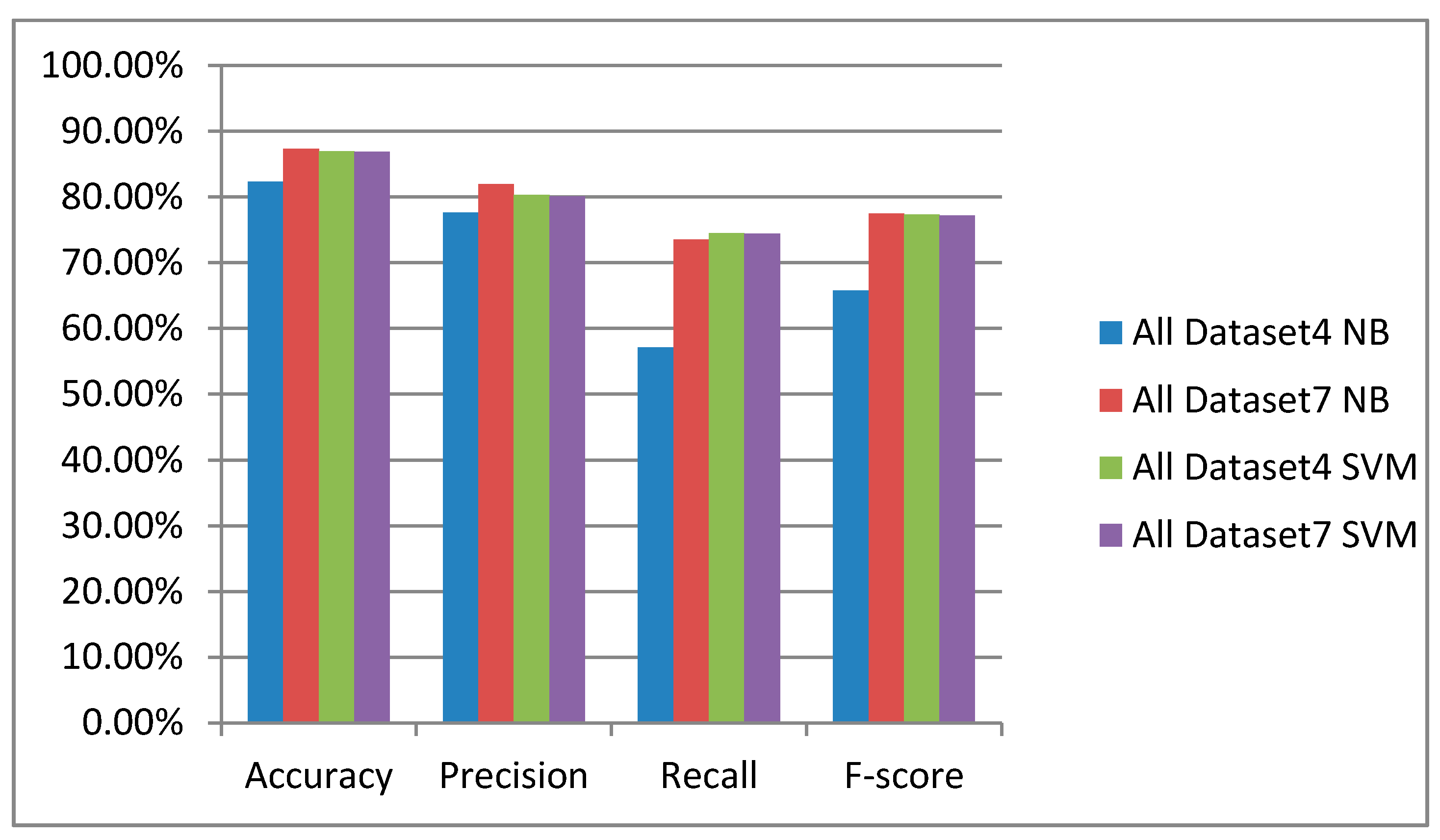
3.3. Comparison of Datasets 4 and 7

Dataset 4 contains 1033 attributes (14 category attributes + 34 subcategory attributes + 985 normalized attributes) and dataset 7 contains 999 attributes (14 category attributes + 985 normalized attributes). Experimental results suggest that both datasets 4 and 7 outperformed dataset 3 used in previous research in the Bordeaux wine application domain. However, drawing the conclusion “the more attributes, the better” is still not very clear. To visualize the experimental results using datasets 4 and 7, Figure 3 is created based on Table 3 and Table 4. 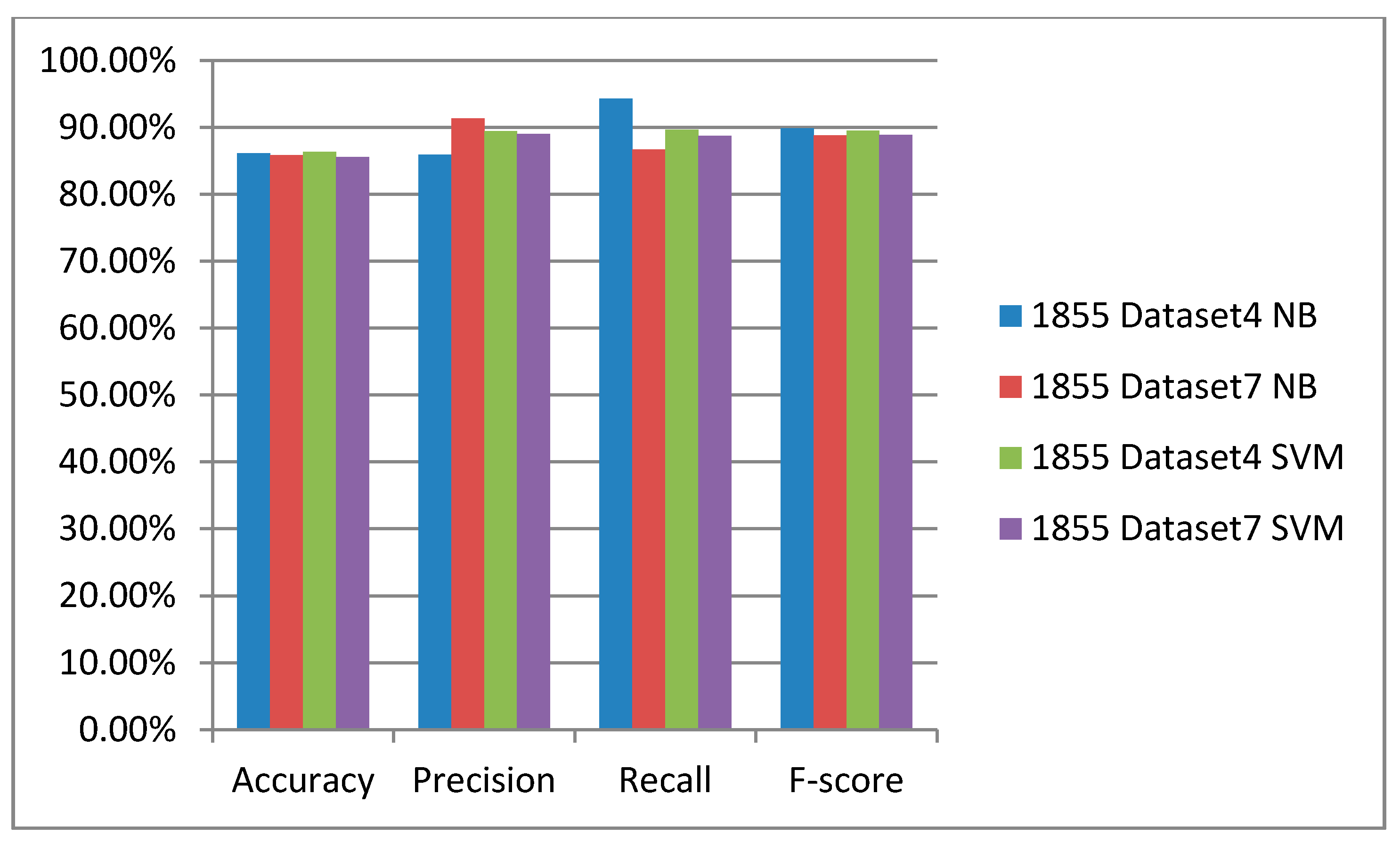Figure 4 is created based on Table 5 and Table 6.

In Figure 3, all results are very similar except dataset 4 using Naïve Bayes. More specifically, the recall performed poorly. In the All-Bordeaux dataset with a total of 14,349 wines, there are 4263 90+ wines and 10,086 89− wines. This imbalanced situation might be the cause for Naïve Bayes to perform poorly in dataset 4, which means the 34 attributes from the SUBCATEGORY cannot provide positive impacts to the model generated from All-Bordeaux wines.

In Figure 4, in terms of accuracy and F-score, both the 1855 datasets 4 and 7 performed very similarly under the SVM and Naïve Bayes algorithms. The only result that needs to be addressed is the recall from the 1855 dataset 4 using Naïve Bayes, which reaches as high as 94%. This result might be affected by the same imbalanced situation of the dataset. In the 1855 Bordeaux dataset with 1359 collected wines, there are 882 90+ wines and 477 89− wines. Unlike the data distribution of the first dataset, which has much more 89− wines than 90+ wines, the 1855 Bordeaux dataset has more 90+ wines than 89− wines. Therefore, we feel dataset 4, which uses all attributes, is more likely to be impacted by the imbalanced dataset. In either case, this research suggests that attributes retrieved from the CATEGORY and SUBCATEGORY have the power to provide more information to classifiers for superior model generation. This finding provides strong impact to many Wineinformatics research efforts in different wine-related topics, such as evaluation on wine reviewers [11], wine grade and price regression analysis [12], terroir study in a single wine region [48], weather impacts examination [49], and multi-target classification on a wine’s score, price, and region [50].

4. Conclusions

In this research, with the full power of the Computational Wine Wheel to extract new attributes from the CATEGORY and SUBCATEGORY, we studied two Bordeaux datasets. The first dataset is all the Bordeaux wine from 2000 to 2016, and the second one is all wines listed in a famous collection of Bordeaux wines, known as the 1855 Bordeaux Wine Official Classification, from 2000 to 2016. Both SVM and Naïve Bayes techniques are utilized to build models for predicting 90+ (Classic and Outstanding wines) and 89− (Very Good and Good wines) wines, and we directly compare the performance with the latest research. According to the results presented in Table 3, Table 4, Table 5 and Table 6, the datasets with additional attributes are able to generate better performance in almost all evaluation metrics. For the All-Bordeaux dataset, with the additional attributes retrieved from the CATEGORY, the Naïve Bayes classification algorithm was able to outperform the existing research results by increasing accuracy by 2.15%, precision by 8.72%, and F-score by 1.48%. For the 1855 Bordeaux dataset, with the additional attributes retrieved from the CATEGORY and SUBCATEGORY, the SVM classification algorithm was able to outperform the existing research results by increasing accuracy by 5%, precision by 2.85%, recall by 5.56%, and the F-score by 4.07%. The improvements demonstrated in the research suggest that attributes retrieved from the CATEGORY and SUBCATEGORY have the power to provide more information to classifiers for superior model generation. The main contributions of this paper are (1) proving a method to process wine reviews through the full power of the Computational Wine Wheel to retain more information and (2) demonstrating how to merge the original binary-attributes and the new continuous-attributes in Wineinformatics data so that the classification models can achieve better performance. This finding provides strong impacts to all Wineinformatics research in many different research topics about wine, which has the potential to provide useful information to wine-makers, consumers, and distributors.