Standardization and Quality Control in Data Collection and Assessment of Threatened Plant Species

Abstract

Informative data collection is important in the identification and conservation of rare plant species. Data sets generated by many small-scale studies may be integrated into large, distributed databases, and statistical tools are being developed to extract meaningful information from such databases. A diversity of field methodologies may be employed across smaller studies, however, resulting in a lack of standardization and quality control, which makes integration more difficult. Here, we present a case study of the population-level monitoring of two threatened plant species with contrasting life history traits that require different field sampling methodologies: the limestone glade bladderpod, Physaria filiformis, and the western prairie fringed orchid, Plantanthera praeclara. Although different data collection methodologies are necessary for these species based on population sizes and plant morphology, the resulting data allow for similar inferences. Different sample designs may frequently be necessary for rare plant sampling, yet still provide comparable data. Various sources of uncertainty may be associated with data collection (e.g., random sampling error, methodological imprecision, observer error), and should always be quantified if possible and included in data sets, and described in metadata. Ancillary data (e.g., abundance of other plants, physical environment, weather/climate) may be valuable and the most relevant variables may be determined by natural history or empirical studies. Once data are collected, standard operating procedures should be established to prevent errors in data entry. Best practices for data archiving should be followed, and data should be made available for other scientists to use. Efforts to standardize data collection and control data quality, particularly in small-scale field studies, are imperative to future cross-study comparisons, meta-analyses, and systematic reviews.

1. Introduction

A recent review [1] estimated that there are 450,000 flowering plant species, a third of which are at risk of extinction. Moreover, current extinction rates were estimated at 1000 to 10,000 times the background rate [1]. The International Union for Conservation of Nature (IUCN) Sampled Red List Index for Plants [2] estimates that one in five plant species are threatened with extinction, with the caveat that a third are so poorly known that it cannot be determined with certainty whether or not they are threatened.

Informative data collection is critical both in identifying which plants are rare and in conservation efforts. Databases such as Tropicos [3], The Biota of North America Program [4], and USDA (United States Department of Agriculture) Plants [5] provide taxonomic information while cataloguing biodiversity. The global distribution information in these databases can be used to identify rare plant species.

Once rare plants are identified, studies often focus on monitoring individual populations. Menges and Gordon [6] provide a framework to characterize these efforts according to sampling effort and intensity (

Table 1. Levels of monitoring rare plants (modified from Menges and Gordon [6]).

Level	Monitoring Intensity	Data Collected
1	Population distribution	Presence/absence, population location
2	Population size	Abundance, geographical extent
3	Demography of individuals	Individual location, characteristics
4	Phenology	Individual characteristics over growing season
	Ancillary variables	Habitat, environment, weather, other species, etc.

). Level 1 focuses on species occurrence by mapping species distributions and obtaining presence/absence information. Level 2 monitoring is designed to quantitatively track changes in the abundance of target populations over time. Level 3 involves demographic monitoring and tracks the fate of individual plants. Phenological monitoring, i.e., recording data at multiple time periods in each growing season (e.g., [7,8]), represents a potential fourth level of sampling intensity. At each level, different methodologies are possible. The ability to account for differences in study design, while pooling the results of multiple studies, would support conservation assessments of rare plant species. Such assessments underlie listing and delisting criteria under the Endangered Species Act.

Requirements for data integration must be met to operate distributed databases. For example, the NatureServe Biodiversity Tracking and Conservation System (BIOTICS) database [9] is a distributed database that documents the location and status of rare plants and animals. The Global Biodiversity Information Facility (GBIF) [10], an international open data infrastructure, provides a single point of access to hundreds of millions of records. The Group on Earth Observations Biodiversity Observation Network (GEO BON) [11,12,13] is a global partnership that assists in the collection, management, analysis, and reporting of data relating to the status of the world’s biodiversity. The Biodiversity Information Standards Taxonomic Databases Working Group (TDWG) [14] was formed to establish international collaboration among biological database projects and focuses on the development of standards for the exchange of biodiversity data.

The call for such harmonization is increasing to encompass not just large, distributed, open access data sets, but also data sets arising from small-scale field studies. There exist many opportunistic records, often simply occurrence data, many of which are shared through the GBIF. Although such data are typically lower in quality than the first tier of Table 1, the sheer number of records may be sufficient to overcome the substantial biases that undoubtedly exist. Statistical tools have been developed to extract meaningful signals from unstructured data [15] and combine them with the results of more structured monitoring [16].

Employing such “big data” tools is expected to encourage the advancement of ecology through data-mining, cross-study analyses/data set integration, meta-analyses, and systematic reviews. Just as distributed data sets depend on common data fields, multi-study data sets must be coded in a way that allows cross-study compatibility. While metadata are essential for interpreting individual data sets, other aspects of the data set can be standardized to prevent misinterpretation and misuse. It is also important to describe the limitations of the data set with respect to the inherent biological, design-, and measurement-based uncertainty.

There exist many different methods of sampling rare plant populations (e.g., [17]), and the most useful methods in any application will depend upon the size of the population, morphology of the plant, background habitat matrix, and other potential factors. The method that provides the most precise estimates for one species may not provide very precise estimates for another, and it is possible that a method that provides precise estimates for a population of a particular species will not be practical for another population of the same species. The ultimate goal should be to obtain the highest quality data that allows for comparability among populations or species, although it is possible that different methods may be necessary. Here, we present a case study of two threatened plant species with contrasting life history traits that require different field sampling methodologies, to illustrate the issues associated with standardization and quality control in integrating smaller scale studies, and how such issues may be resolved.

2. Data Collection

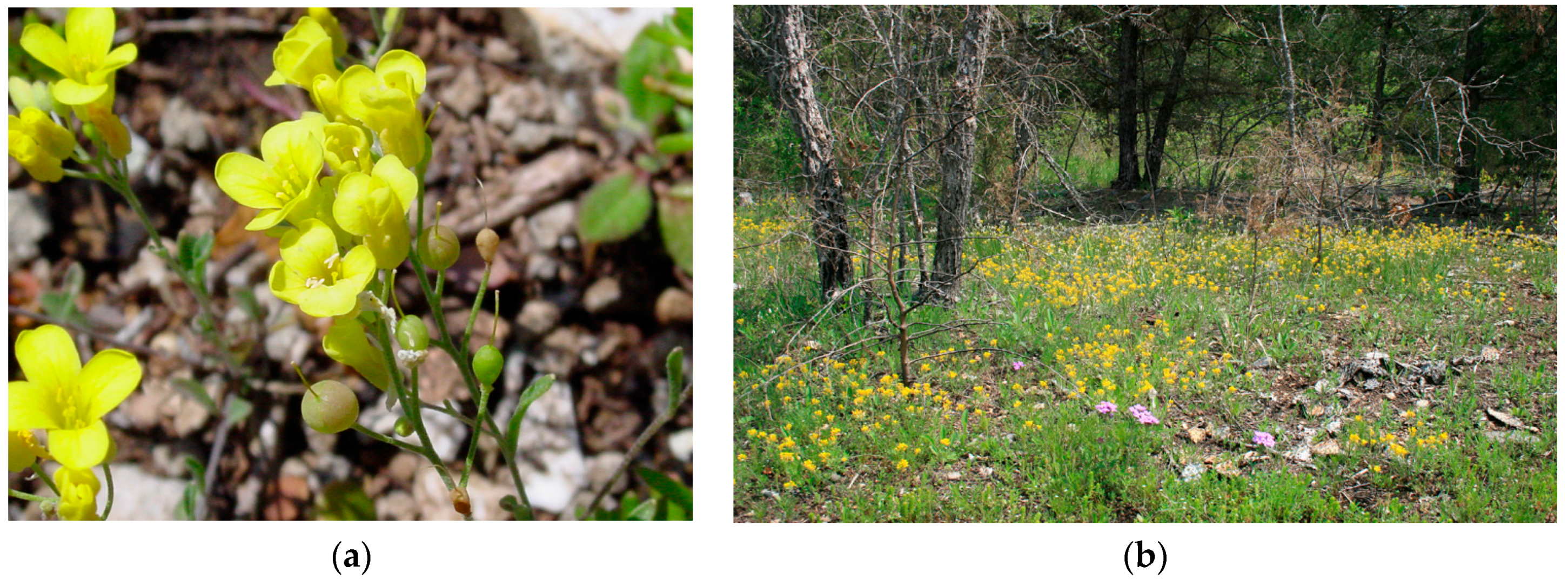
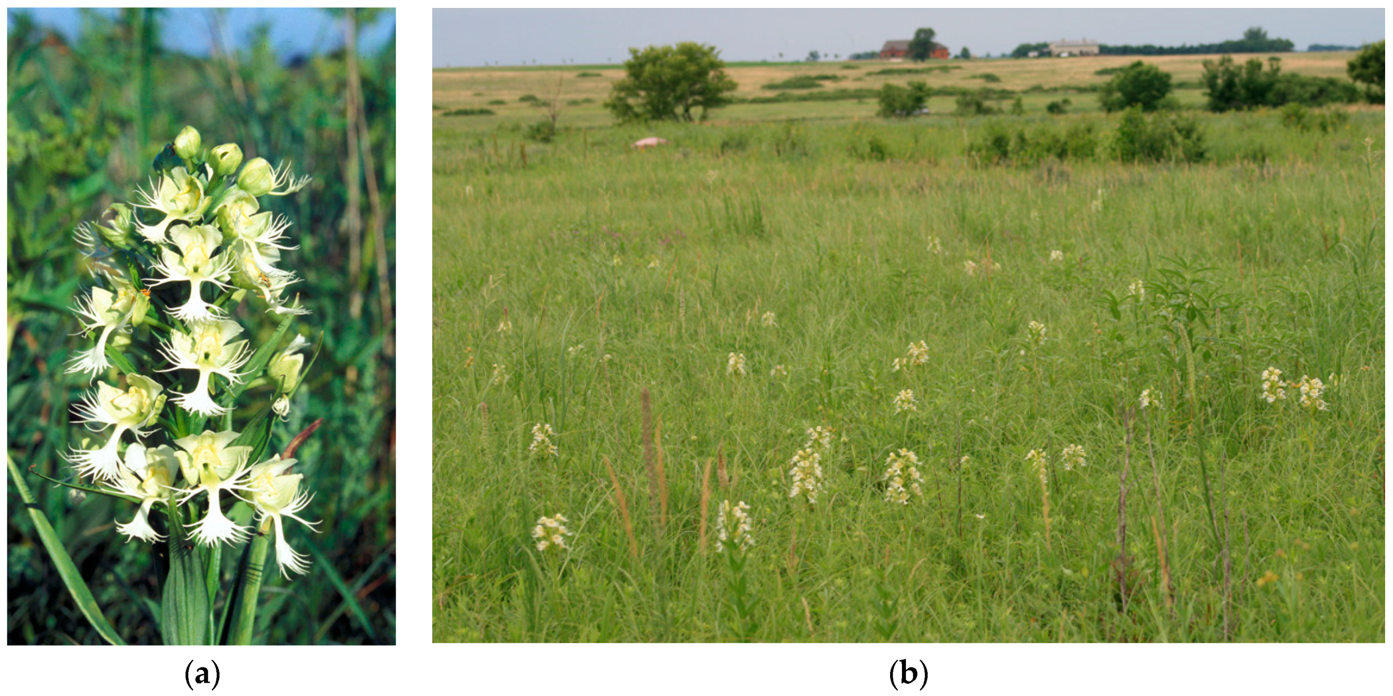
As an example of smaller scale data sets, the Heartland Network of the National Park Service’s Inventory and Monitoring Program (NPS I&M) monitors two threatened plant species: the limestone glade bladderpod, Physaria filiformis (Rollins) O’Kane and Al-Shehbaz (Figure 1), and the western prairie fringed orchid, Plantanthera praeclara Sheviak and Bowles (Figure 2). Primary objectives include estimation of population abundance (e.g., level 2 monitoring). Detailed monitoring protocols, along with standard operating procedures for data collection and management, have been developed for both the bladderpod [18] and the orchid [19]. Although the goals for conservation of the two species are similar, standard operating procedures vary due to differences in the two species’ natural history and their population sizes.

The limestone glade bladderpod is a winter annual in the mustard family found in limestone, dolomite, and shale glades in Alabama, Arkansas, and Missouri [20]. The bladderpod germinates in late summer to autumn and overwinters as a rosette. It produces yellow flowers with 5–9 mm petals in April–May, sets seed, and senesces by late spring. Each rosette may support multiple flowering stems up to 25 cm in height. A substrate endemic, the bladderpod is rare and listed by the U.S. Fish and Wildlife Service as a threatened species [21].

The western prairie fringed orchid is a perennial, herbaceous orchid found in tallgrass prairies from south-central Canada through the western central lowlands and eastern Great Plains of the United States [22]. The orchid typically emerges in mid-April to late May. Two above ground growth forms exist: vegetative, with only a few leaves, and flowering. Four different vegetative stage classes have been described [7]. Flowering plants support inflorescences consisting of a spike of up to 30 creamy white flowers, 38–85 cm tall [23]. Individual flowers persist for up to ten days, and a single large inflorescence may produce flowers for up to three weeks [24]. A relatively large proportion of the population may be dormant or vegetative in any given year. The orchid is declining due to prairie conversion and alteration of hydrological regimes associated with agricultural modification [22] and is listed as threatened [25].

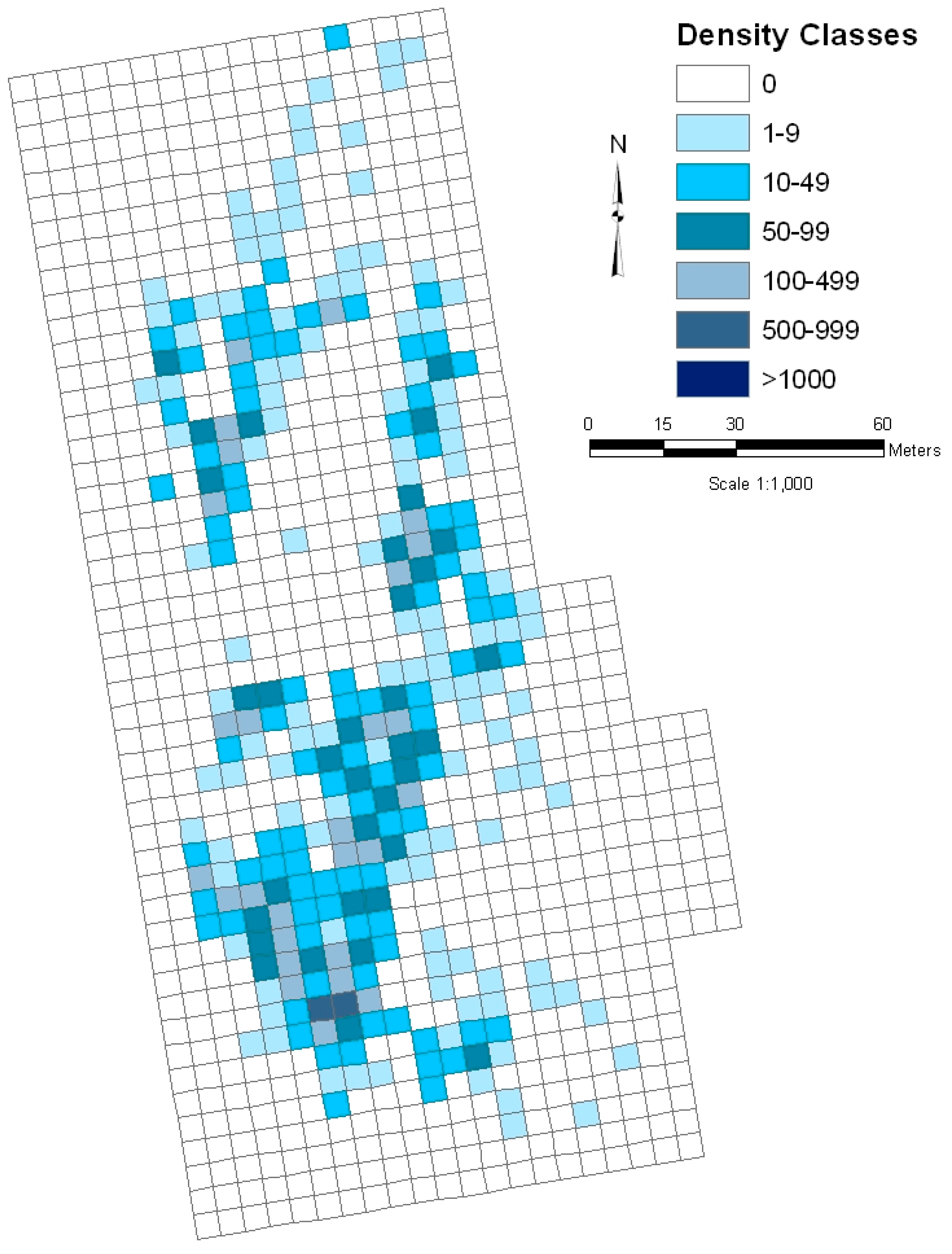
Field data collection in monitoring the bladderpod involves partitioning of the population into a grid of 5 × 5 m cells, and estimating abundances for each cell within seven density classes (0; 1 = 1–9; 2 = 10–49; 3 = 50–99; 4 = 100–499; 5 = 500–999; and 6 = 1000–4999). The use of density classes, rather than counts, is necessitated by the small size and variable growth form (multiple branching stems), combined with potentially high abundances. Population size is estimated by summing the low and high ends of the estimated density class assigned to each occupied cell, to calculate an overall population size interval [18]. The advantage of this method is that it provides spatial information for the entire population, allowing mapping of the glade to illustrate where plants are clustered (Figure 3). Unlike a traditional sampling approach, in which there exists uncertainty in any point estimate due to random error, there is an inherent uncertainty in point estimates due to the use of density classes. The calculated population size interval is analogous to a 100% confidence interval. The width of the interval, for the bladderpod population sampled, is very similar to that of a 95% confidence interval calculated in the traditional fashion based on a simple random sample [26].

In contrast, field data collection in the orchid is accomplished by a systematic search involving a team of four to eight observers walking in tandem 2 m apart [19,27]. Locations of flowering orchids are recorded with a GPS unit; the accuracy of GPS positions is within 2 m. Plant height and the numbers of flowers or buds are also recorded. Sampling occurs during peak flowering, which is almost always in July. Thus, data collection in orchid monitoring represents a census, rather than a sample, of all flowering orchids in the population. Such an approach is possible because of the relatively low abundances of this population and the relatively small area over which it occurs.

Abundance of both species varies dramatically. Over a two-decade period, the number of flowering plants in an orchid population in southwestern Minnesota ranged between 0 and 722 [28]. Other orchid populations have also demonstrated high inter-annual variability [7,29]. In one bladderpod population in southwestern Missouri that has been monitored annually over an 18 year period, population size of flowering plants ranged between 0 and 262,000 [30].

In both species, the probability of detecting non-flowering plants varies due to the annual and perennial life cycles. In the bladderpod, presumably an extremely high percentage of rosettes that survive the winter will produce flowering stems in the spring [31]. In any case, all individuals present in April will be absent in the subsequent year. A seed bank of unknown size allows for a rapid population increase when environmental conditions are appropriate. While blooming bladderpod plants are the most detectable, non-blooming stems (in the bud or fruit stage) can also be readily located.

In the case of the orchid, in addition to a seed bank of unknown size, orchids may also persist as dormant or vegetative individuals. Due to the tallgrass cover in prairies, this stage is virtually undetectable without carefully combing through the vegetation. A relatively large proportion of plants may be dormant or vegetative in any given year [24]. Flowering plants may transition to vegetative plants and vice versa [7]. Flowering plants in bloom are more highly detectable than plants in bud or fruit, although both can be detected readily.

3. Sample Design

The extent of data collected in any project will depend upon the sampling frame [32]. The sampling frame represents the target population, although it is rarely an exact representation. Not all individuals in the population may be included in the sampling frame, for example. In the bladderpod population, 963 5 × 5 m cells have been established over the glade and include virtually all bladderpod plants. Many of the cells along the periphery contain marginal habitat and few bladderpods, so that a smaller core area of 477 cells is sampled annually, and all 963 cells are sampled infrequently. Thus, in the interest of sampling efficiency, the reference frame does not encompass the entire bladderpod population, but approximately 95% of it (in 2015). As long as the same area is sampled consistently, meaningful comparisons may be made, even if it is not practical to sample the entire population.

The size of the population, as well as the variability in size, are important considerations in determining the sample design. Populations that are consistently small could be completely censused (i.e., each individual counted). Large populations, or populations that are extremely variable over time, usually must be sampled (i.e., some random fraction of the population counted). A census would provide the most precise information (in the absence of observer error); under ideal conditions an exact count may be possible. A sample, in contrast, will always yield uncertainty due to random error (i.e., the fraction of the population sampled may not be representative). The orchid population is small enough so that it can be consistently censused, whereas the bladderpod population is too large in many years.

If a population is large enough or variable enough so that sampling is necessary, a diversity of sample designs may be applied, depending upon various factors. In the case of the bladderpod, which exhibits some clustering, numerous sample designs have been evaluated in the field and in computer simulations, including a simple random sample, systematic sampling, and several types of adaptive sampling [30]. The relative efficiencies of various sample designs may be difficult to evaluate; computer simulations may be useful in determining the relative efficiencies [30].

In the case of the bladderpod, it was determined to employ the approach of estimating the abundance of each cell within density classes, as this provided broad spatial information that would not be obtained from sampling a subset of the population [18]. Thus, because all cells in the core area are included, there is no statistical uncertainty due to random sampling error. There is, however, uncertainty due to other sources: width of the density classes [26] and observer error [33]. Thus, the magnitude of any source of uncertainty should always be quantified and included in the data set. In general, the use of different designs does not necessarily result in incomparable data sets, particularly as long as the uncertainties associated with the estimates are provided.

4. Ancillary Data

In addition to population-level data on the target plant species, information may also be desired for various ancillary variables, such as the abundance of other plants, the physical environment, or weather/climate. The orchid, for example, is usually found in mesic swales or draws, and soil moisture appears to affect dormancy and flowering in this species [24,29,34,35]. Ancillary data collected for the orchid includes cumulative precipitation within six phenological stages of the orchid [36]. Because of the presumed importance of soil moisture, data on precipitation (which is more readily obtained) has been used in modeling efforts [28,37] and analyses of empirical data [29]. Data on temperature within these stages and on snow depth for various time periods have also been incorporated into models [38]. As a result of knowledge of orchid phenology [36], there exists some standardization on relevant time periods in the various modeling efforts.

Ancillary data collected for the bladderpod consist of estimates of the percent cover of exotic plant species, measurement of the basal diameter of Eastern redcedar (Juniperus virginiana), a species that encroaches upon glade habitat, and measurement of the photosynthetically active radiation. These data have been used in attempts to explain the spatial distribution of the bladderpod and evaluate the effects of management actions [39].

5. Data Quality Control

An important component of the data describing rare plant populations is related to the uncertainty associated with point estimates. Such uncertainty may be due to at least three sources of error: (1) Random error exists any time data are collected by a sampling process; (2) Methodological uncertainty occurs when the sampling process is not precise (e.g., the use of density classes rather than specification of absolute densities); (3) Observer error occurs due to the inability to precisely quantify vegetation subjectively. The magnitudes of random error and methodological uncertainty are easily calculated from basic information. Determination of the existence and magnitude of observer error will usually require additional data collection in the field.

Data collected by human observers will almost always be characterized by some degree of observer error. A recent review [40] found that 92% of vegetation studies employing observers that tested for a statistical effect of observer error found at least one significant comparison. The magnitude of error was often as much as 20% to 30% of the estimated value of the parameter. Observer error arises when different observers do not arrive at similar estimates (inter-observer error) or when the same observer does not provide similar estimates over time (intra-observer error). The use of digital imagery techniques may provide more precise estimates than human observers, although is more time-consuming. Moreover, different digital imagery techniques yield different results [41]. In many cases, photographic techniques may produce imprecise estimates, for example when layers of vegetation are present, or shading obscures vegetation features [42]. Thus, human observers are frequently the most cost-effective option.

In the orchid population, the relatively large, showy plants are difficult for observers to miss. Some observer error may exist, although it is likely to be trivial. In the bladderpod population, in contrast, the relatively small size, existence of multiple branching stems, and dense concentrations of the plants makes observer error likely, even with the use of density classes. Observer error has been quantified in the sampling of this population by counting ~10% the cells after estimates within density classes were made. Over a third of the cells (36.4%) were not estimated correctly [33]. Most (29.4%) were underestimates by one density class. Underestimates became more prevalent as density class increased. Because the errors represent a systematic bias, it is possible to employ a correction factor to the data [26]. Inherent differences were found to exist among observers, however, that could not be explained by experience or training. Thus, correction factors would ideally need to be both density class-dependent and observer-specific [33].

Another potential source of error in both species is related to the time of sampling. In both species, individual plants are difficult to observe in the absence of flowering stems, so sampling is timed to coincide with peak flowering. If sampling occurs before or after peak flowering, or flowering is not synchronized among the plants within the population, non-flowering individuals may not be observed. Such error is difficult to quantify in the absence of phenological monitoring.

Once data are collected, quality measures should be established to prevent errors in data entry. In the case of the orchid and bladderpod, such data quality measures include data entry practices as well as features that are built into the database [18,19]. First, data entry is controlled through a graphic user interface (GUI), which prevents direct access to the data tables. Such access could lead to inadvertent changes in the data. Within the GUI, data entry is also controlled through pick-lists that restrict the data input to the range of potential values. For example, density classes for the bladderpod range from 0 to 6; only integers in this range are acceptable inputs. The study period and habitat cover classes are similarly controlled. While these measures restrict the potential for error, entry of values that are feasible yet incorrect is still possible. To minimize such mistakes, we perform a 100% check of the data following initial entry in the database. Next, we perform a verification of 10% of the data. If any mistakes are found during this review, this triggers another round of a 100%-check and 10%-verification. While such measures cannot guarantee accurate data entry, they will reduce or eliminate certain types of error.

6. Summary of Data Collected and Comparisons with Other Studies

In the case of the orchid, the primary data set consists of the number of flowering orchids as determined by a census, the height of each plant, the number of flowers or buds on each plant, and the location of each plant, in each year (

Table 2. Types of data collected in the field and summarized from field data collection for two rare plant species. Variables in italics represent ancillary variables.

Data Collected in Field	Population-Level Data (Summarized)
Western prairie fringed orchid 1
Individual plant height	Total abundance
Number of flowers/buds	Mapping of individuals
Individual plant location	Precipitation 2
Missouri bladderpod 3
Density class of cell	Total abundance 4
Photosynthetically active radiation	Adjusted total abundance 4,5
Eastern redcedar basal area	Mapping of relative densities
Percent cover of exotic species

¹ field measurements made on individual plants; ² data obtained from local weather stations; ³ field measurements made on 5 × 5 m cells; ⁴ including uncertainty based on the use of density classes; ⁵ including correction factor to compensate for observer error.

). There exists no uncertainty due to random sampling error, and observer error is likely to be trivial. The location of individual orchids can be very accurately mapped [28]. Demographic work has been conducted to a limited extent in this orchid population [43].

In the case of the bladderpod, the primary data set consists of an estimate of the number of plants for each cell (Table 2). Although there exists no uncertainty due to random sampling error, there is uncertainty related to the width of the density class. Observer error is of a relatively large magnitude, and can be corrected for the overall population estimate, but not for individual cells. Spatial variation in the density of the bladderpods can be mapped across the glade at the resolution of the 5 × 5 m cells [26]. Limited demographic data have been collected in this population, including a two-year study evaluating winter survivorship [31].

A number of western prairie fringed orchid populations in Minnesota are monitored by the Minnesota Department of Natural Resources (DNR) by the application of a nested monitoring protocol, which is similar to the three levels of Menges and Gordon [6] plus phenological monitoring. The first level (presence/absence mapping) includes all known populations. Because greater effort is required at each higher level, progressively fewer sites are included. The second level is a census of all flowering plants, which is conducted at 80% of the populations. The more intensive demographical and phenological levels are evaluated at only a few sites [7]. Presence/absence information is tracked in the BIOTICS database [9]. The standardized methodology employed by the Minnesota DNR allows comparisons to be made among the orchid populations in Minnesota and their annual censuses of flowering plants are directly comparable to our NPS I&M work.

We are not aware of any other long-term bladderpod data sets with annual observations. The BIOTICS database maintains long-term records on the location of bladderpod populations in Arkansas and Missouri.

7. Implications for Data Collection in Other Rare Plant Species

Monitoring rare plant populations may often involve small-scale field studies conducted by multiple researchers. Data collection will depend upon factors such as the amount of time and funding available for sampling, as well as the distribution, life history traits, and population size of the target species. In many cases, the focus will probably be on estimation of population abundance (e.g., level 2 monitoring). As we have demonstrated here, different sampling methodologies may be necessary, although such efforts need not be disparate. Rather, different sampling techniques can produce comparable data, although care should be taken to maximize comparability. If some data are available, computer simulations may be useful in selecting the most efficient sample design.

Unfortunately, ecologists receive little or no training in data management and many are not familiar with the best practices in data archiving [44]. A recent study found that out of 100 surveyed data sets, 56% were incomplete, due to missing data or insufficient metadata, and 64% were archived in a way that hampered reuse [44]. In addition to a lack of training, a larger problem appears to be cultural: many ecologists simply view their data as precursors to publications rather than enduring products of research, effectively failing to contribute to broader scientific efforts [45]. Although the benefits of public data archiving to the larger scientific community may outweigh the costs involved, it is less obvious that the benefits outweigh the costs for individual researchers [46]. In a survey of studies funded by the National Science Foundation’s Division of Environmental Biology, for example, only 8% of published studies made public any of their non-genetic data [45]. Although it has been argued that scientists have an ethical obligation to share data, important aspects of such sharing, including appropriate citation and co-authorship practices, are not widely agreed upon [47].

What can ecologists do to promote standardization in rare plant studies and increase the likelihood that their data will be useful to the larger scientific community? We offer several suggestions: (1) Become familiar with similar studies of rare plants, including the types of ancillary variables considered and the spatial scale of data collection. Limited budgets or differing life histories may preclude duplication of sampling methods, although as described above comparable data may be collected; (2) Make the necessary efforts to ensure resulting data are available for others to use. Many journals allow archiving of data as electronic appendices, and data may be published through large data networks such as GEO BON. For threatened or endangered species, location data may be restricted, although data on other aspects of these populations should be made available; (3) Use best practices for data archiving, including complete metadata. Several contributions in the literature describe these best practices [48,49,50]; (4) Evaluate and provide information on the quality of the data. Observer error is ubiquitous in vegetation sampling, and it is important to quantify such error before valid inferences can be made. Quantification of observer error will usually require additional data collection and should be considered in the planning process.

Ultimately, the objectives of any study should include the collection of high quality, standardized data that allows for comparisons among published small-scale studies conducted by multiple investigators at different times. Furthermore, properly archived data will allow for formal meta-analyses or other big data projects. These two goals are not mutually exclusive, and could be obtained by the appropriate planning and willingness to share information. The above considerations are not unique to rare plant sampling, and could be applied more generally to most ecological studies.