Machine-Learning Models for Sales Time Series Forecasting †

1
SoftServe, Inc., 2D Sadova St., 79021 Lviv, Ukraine
2
Ivan Franko National University of Lviv, 1, Universytetska St., 79000 Lviv, Ukraine
†
This paper is an extended version of conference paper: Bohdan Pavlyshenko. Using Stacking Approaches for Machine Learning Models. In Proceedings of the 2018 IEEE Second International Conference on Data Stream Mining & Processing (DSMP), Lviv, Ukraine, 21–25 August 2018.
Data 2019, 4(1), 15; https://0-doi-org.brum.beds.ac.uk/10.3390/data4010015
Submission received: 3 November 2018
/
Revised: 9 January 2019
/
Accepted: 14 January 2019
/
Published: 18 January 2019
(This article belongs to the Special Issue Data Stream Mining and Processing)
Abstract
:In this paper, we study the usage of machine-learning models for sales predictive analytics. The main goal of this paper is to consider main approaches and case studies of using machine learning for sales forecasting. The effect of machine-learning generalization has been considered. This effect can be used to make sales predictions when there is a small amount of historical data for specific sales time series in the case when a new product or store is launched. A stacking approach for building regression ensemble of single models has been studied. The results show that using stacking techniques, we can improve the performance of predictive models for sales time series forecasting.
1. Introduction
Sales prediction is an important part of modern business intelligence [1,2,3]. It can be a complex problem, especially in the case of lack of data, missing data, and the presence of outliers. Sales can be considered as a time series. At present time, different time series models have been developed, for example, by Holt-Winters, ARIMA, SARIMA, SARIMAX, GARCH, etc. Different time series approaches can be found in [4,5,6,7,8,9,10,11,12,13,14,15]. In [16] authors investigate the predictability of time series, and study the performance of different time series forecasting methods. In [17], different approaches for multi-step ahead time series forecasting are considered and compared. In [18], different forecasting methods combining have been investigated. It is shown that in the case when different models are based on different algorithms and data, one can receive essential gain in the accuracy. Accuracy improving is essential in the cases with large uncertainty. In [19,20,21,22,23,24], different ensemble-based methods for classification problems are considered. In [25], it is shown that by combining forecasts produced by different algorithms, it is possible to improve forecasting accuracy. In the work, different conditions for effective forecast combining were considered. In [26] authors considered lagged variable selection, hyperparameter optimization, comparison between classical algorithms and machine learning based algorithms for time series. On the temperature time series datasets, the authors showed that classical algorithms and machine-learning-based algorithms can be equally used. There are some limitations of time series approaches for sales forecasting. Here are some of them:
- We need to have historical data for a long time period to capture seasonality. However, often we do not have historical data for a target variable, for example in case when a new product is launched. At the same time we have sales time series for a similar product and we can expect that our new product will have a similar sales pattern.
- Sales data can have a lot of outliers and missing data. We must clean outliers and interpolate data before using a time series approach.
- We need to take into account a lot of exogenous factors which have impact on sales.
Sales prediction is rather a regression problem than a time series problem. Practice shows that the use of regression approaches can often give us better results compared to time series methods. Machine-learning algorithms make it possible to find patterns in the time series. We can find complicated patterns in the sales dynamics, using supervised machine-learning methods. Some of the most popular are tree-based machine-learning algorithms [27], e.g., Random Forest [28], Gradiend Boosting Machine [29,30]. One of the main assumptions of regression methods is that the patterns in the past data will be repeated in future. In [31], we studied linear models, machine learning, and probabilistic models for time series modeling. For probabilistic modeling, we considered the use of copulas and Bayesian inference approaches. In [32], we studied the logistic regression in the problem of detecting manufacturing failures. For logistic regression, we considered a generalized linear model, machine learning and Bayesian models. In [33], we studied stacking approaches for time series forecasting and logistic regression with highly imbalanced data. In the sales data, we can observe several types of patterns and effects. They are: trend, seasonality, autocorrelation, patterns caused by the impact of such external factors as promo, pricing, competitors’ behavior. We also observe noise in the sales. Noise is caused by the factors which are not included into our consideration. In the sales data, we can also observe extreme values—outliers. If we need to perform risk assessment, we should to take into account noise and extreme values. Outliers can be caused by some specific factors, e.g., promo events, price reduction, weather conditions, etc. If these specific events are repeated periodically, we can add a new feature which will indicate these special events and describe the extreme values of the target variable.
In this work, we study the usage of machine-learning models for sales time series forecasting. We will consider a single model, the effect of machine-learning generalization and stacking of multiple models.
2. Machine-Learning Predictive Models
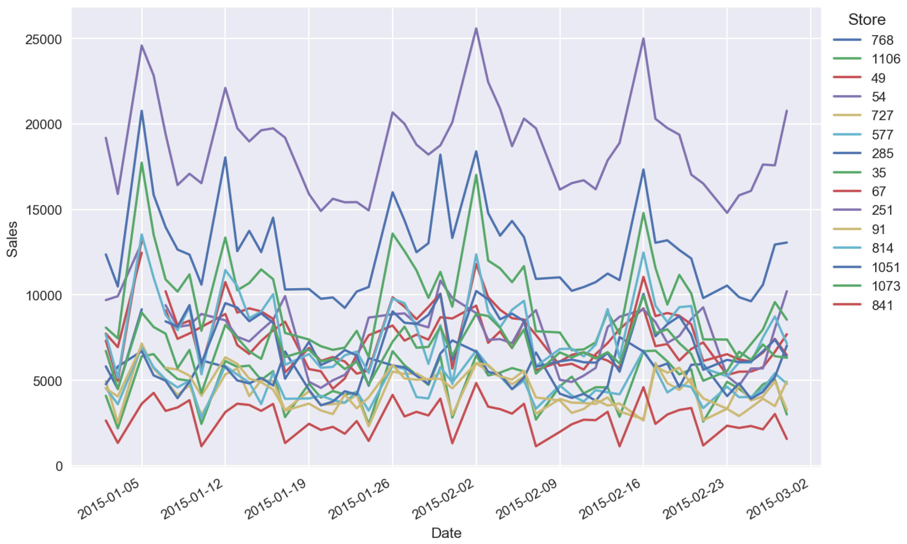
For our analysis, we used store sales historical data from “Rossmann Store Sales” Kaggle competition [34]. These data describe sales in Rossmann stores. The calculations were conducted in the Python environment using the main packages pandas, sklearn, numpy, keras, matplotlib, seaborn. To conduct the analysis, Jupyter Notebook was used. Figure 1 shows typical time series for sales, values of sales are normalized arbitrary units.
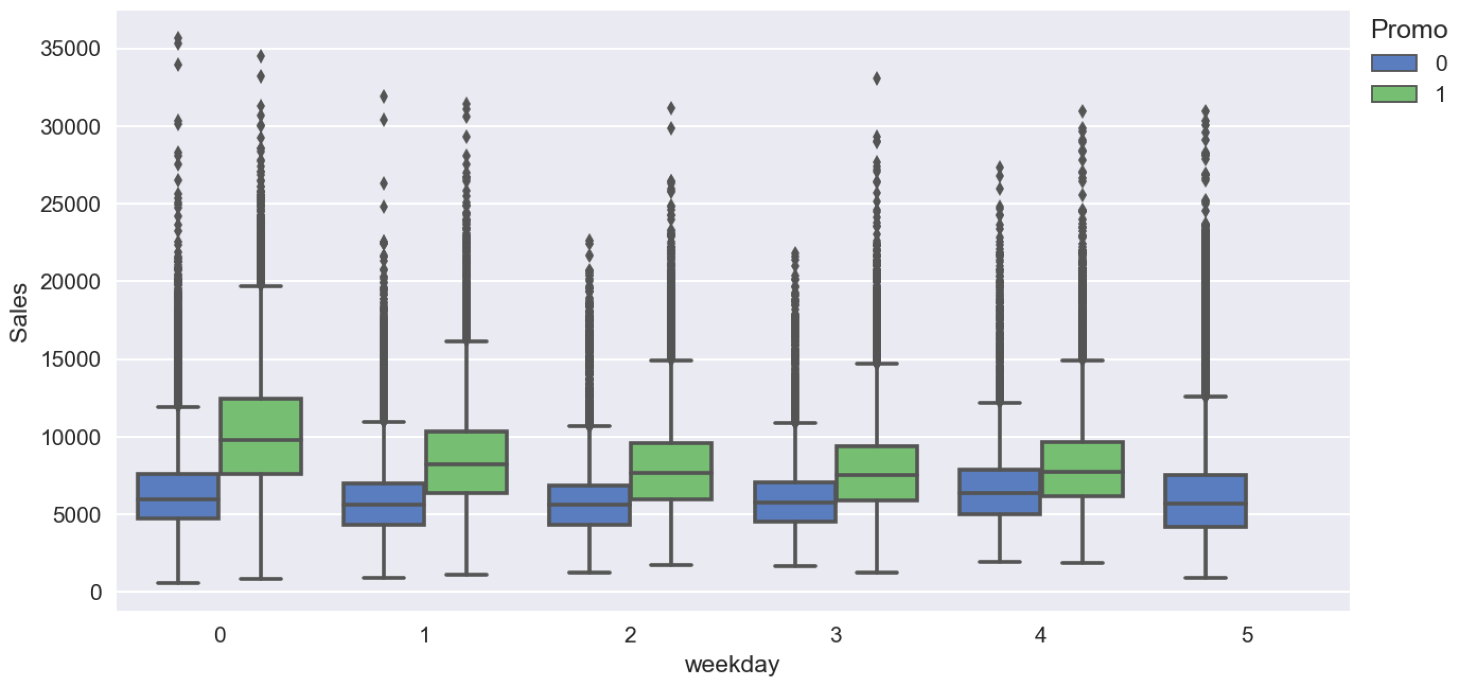
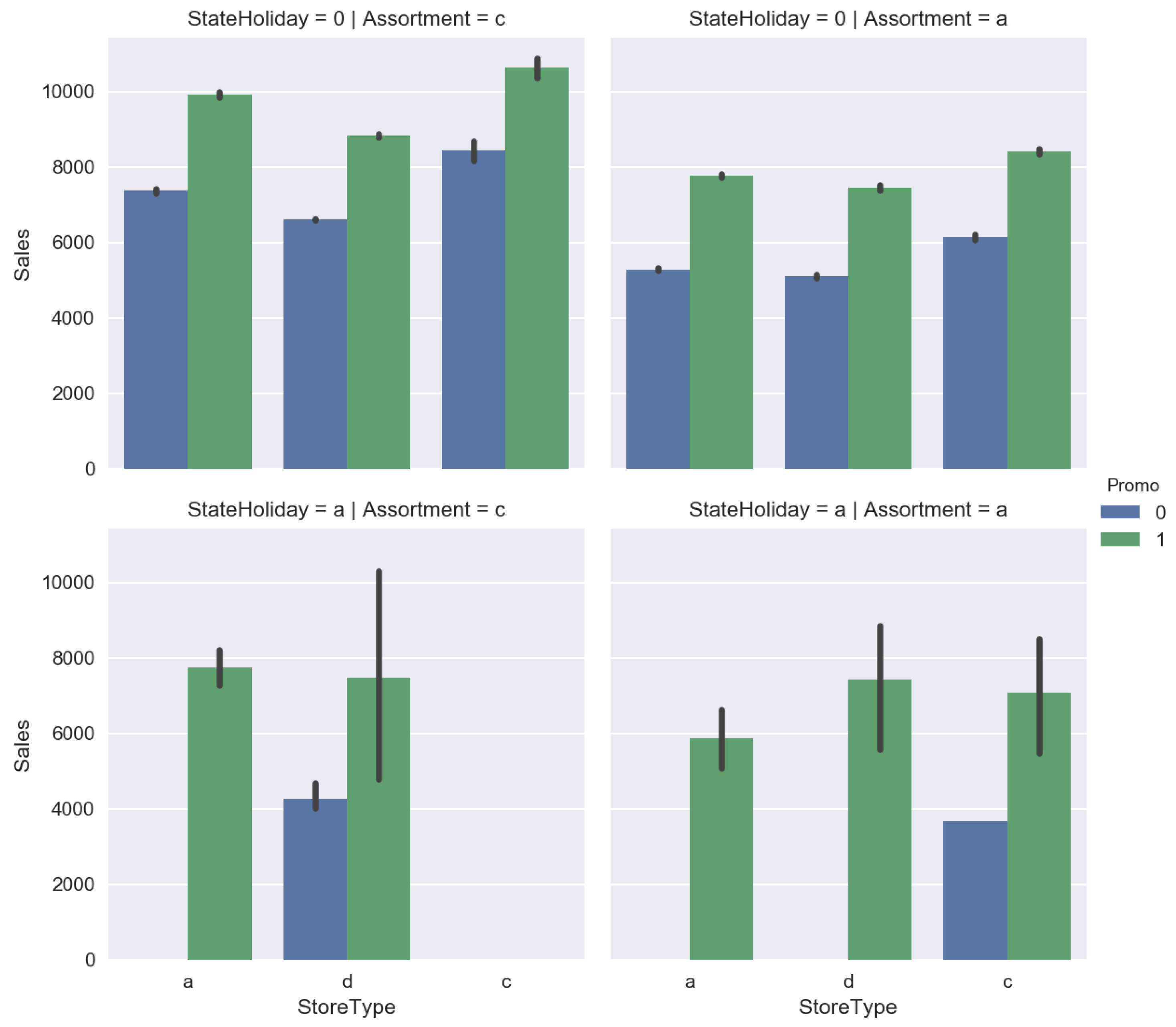
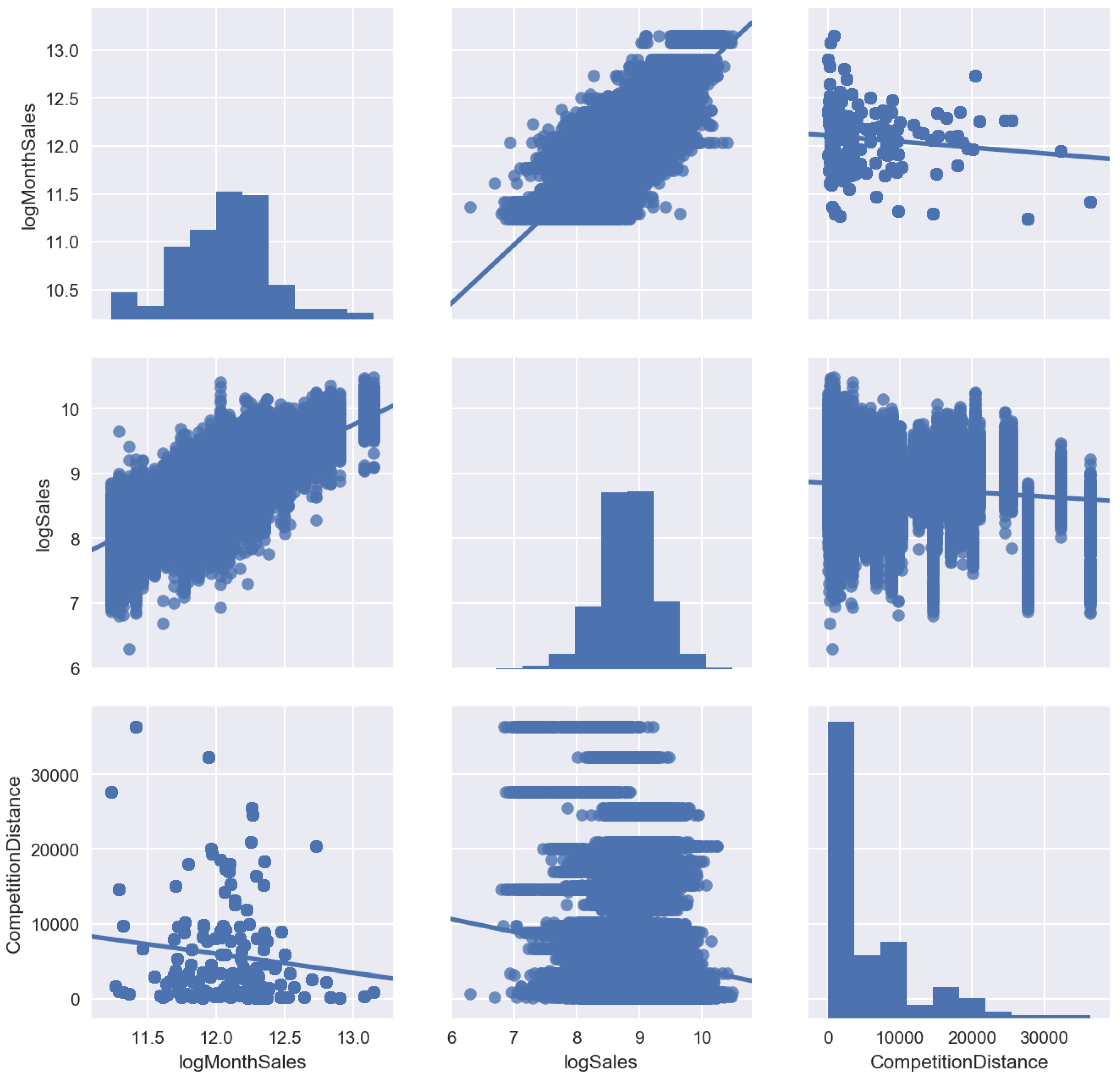
Firstly, we conducted the descriptive analytics, which is a study of sales distributions, data visualization with different pairplots. It is helpful in finding correlations and sales drivers on which we focus. Figure 2, Figure 3 and Figure 4 show the results of the exploratory analysis.
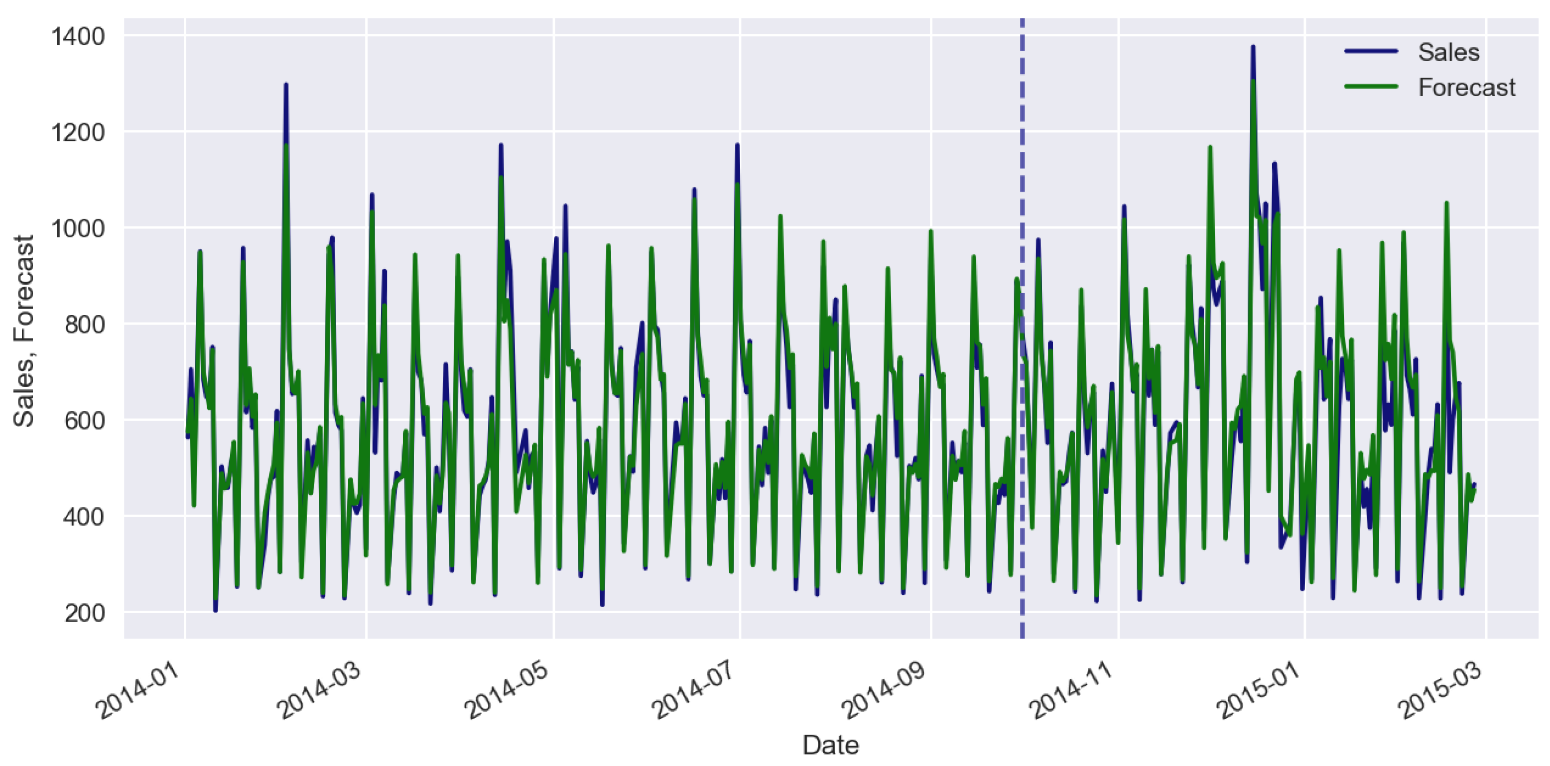
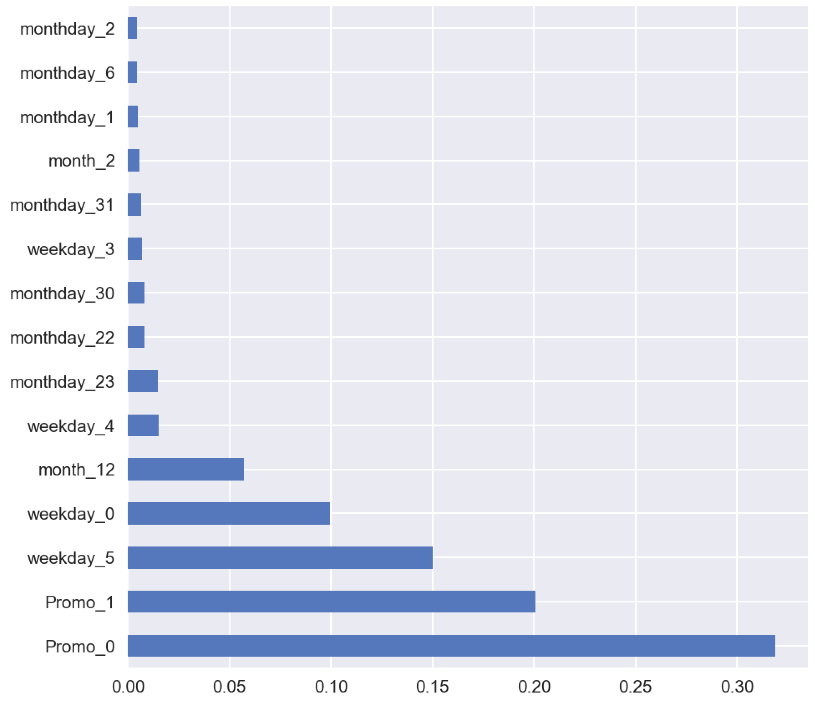
A specific feature of most machine-learning methods is that they can work with stationary data only. In case of a small trend, we can find bias using linear regression on the validation set. Let us consider the supervised machine-learning approach using sales historical time series. For the case study, we used Random Forest algorithm [28]. As covariates, we used categorical features: promo, day of week, day of month, month. For categorical features, we applied one-hot encoding, when one categorical variable was replaced by n binary variables, where n is the amount of unique values of categorical variables. Figure 5 shows the forecasts of sales time series. Figure 6 shows the feature importance. For error estimation, we used a relative mean absolute error (MAE) which is calculated as .
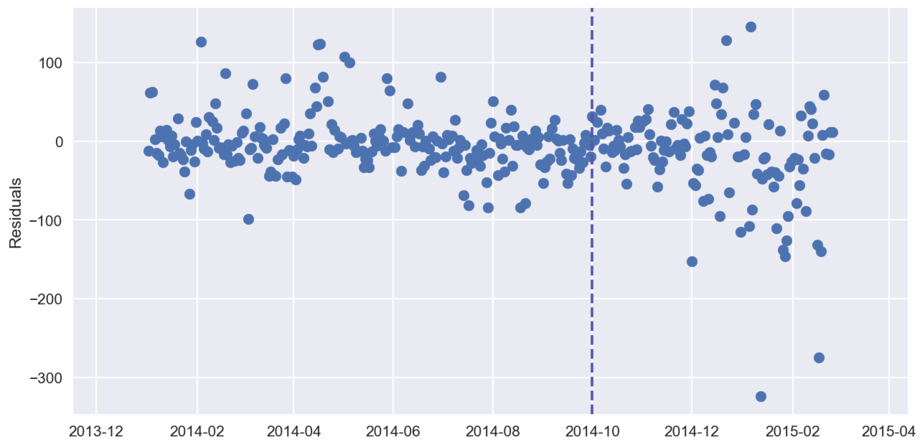
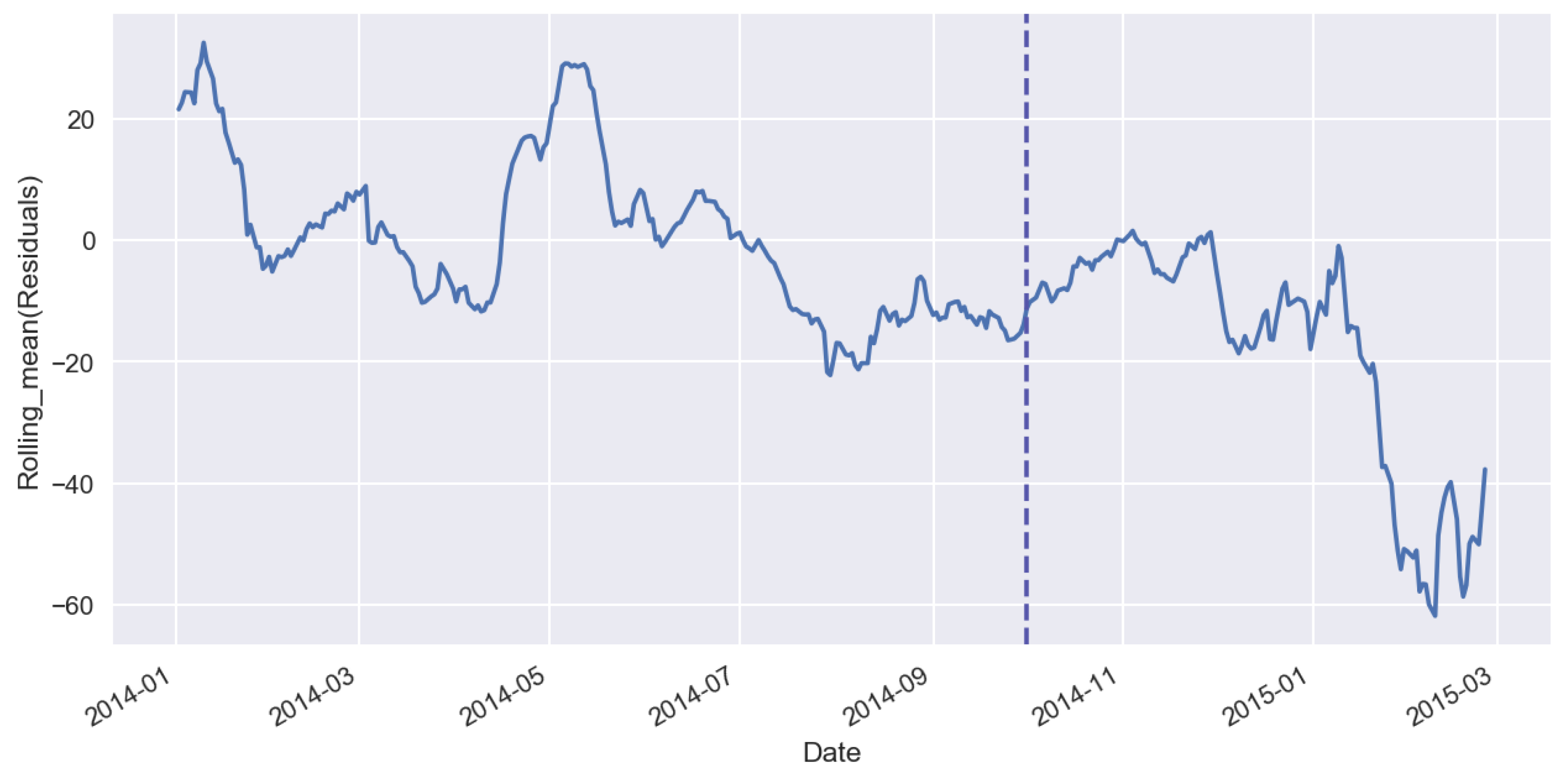
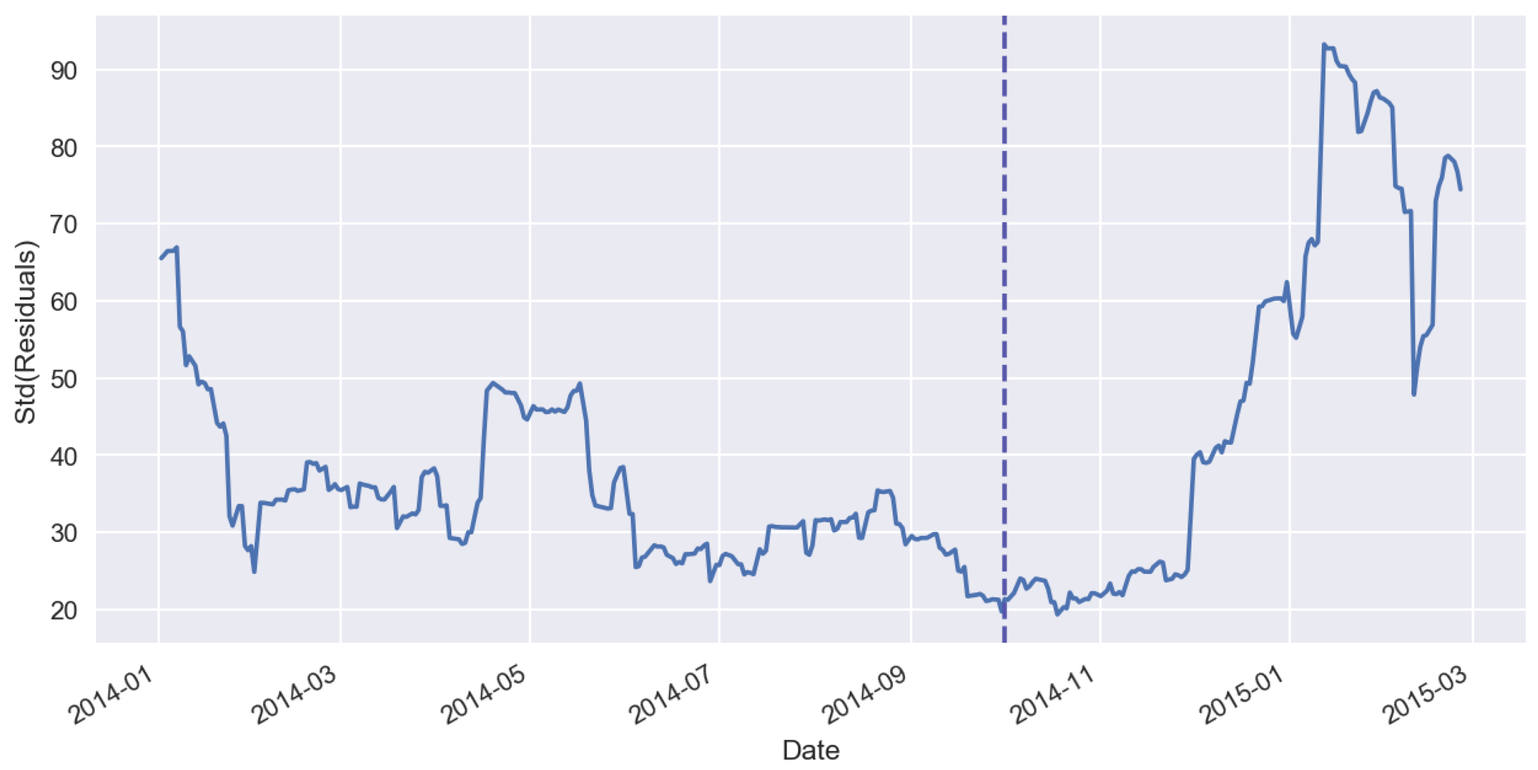
Figure 7 shows forecast residuals for sales time series, Figure 8 shows the rolling mean of residuals, Figure 9 shows the standard deviation of forecast residuals.
In the forecast, we may observe bias on validation set which is a constant (stable) under- or over-valuation of sales when the forecast is going to be higher or lower with respect to real values. It often appears when we apply machine-learning methods to non-stationary sales. We can conduct the correction of bias using linear regression on the validation set. We must differentiate the accuracy on a validation set from the accuracy on a training set. On the training set, it can be very high but on the validation set it is low. The accuracy on the validation set is an important indicator for choosing an optimal number of iterations of machine-learning algorithms.
3. Effect of Machine-Learning Generalization
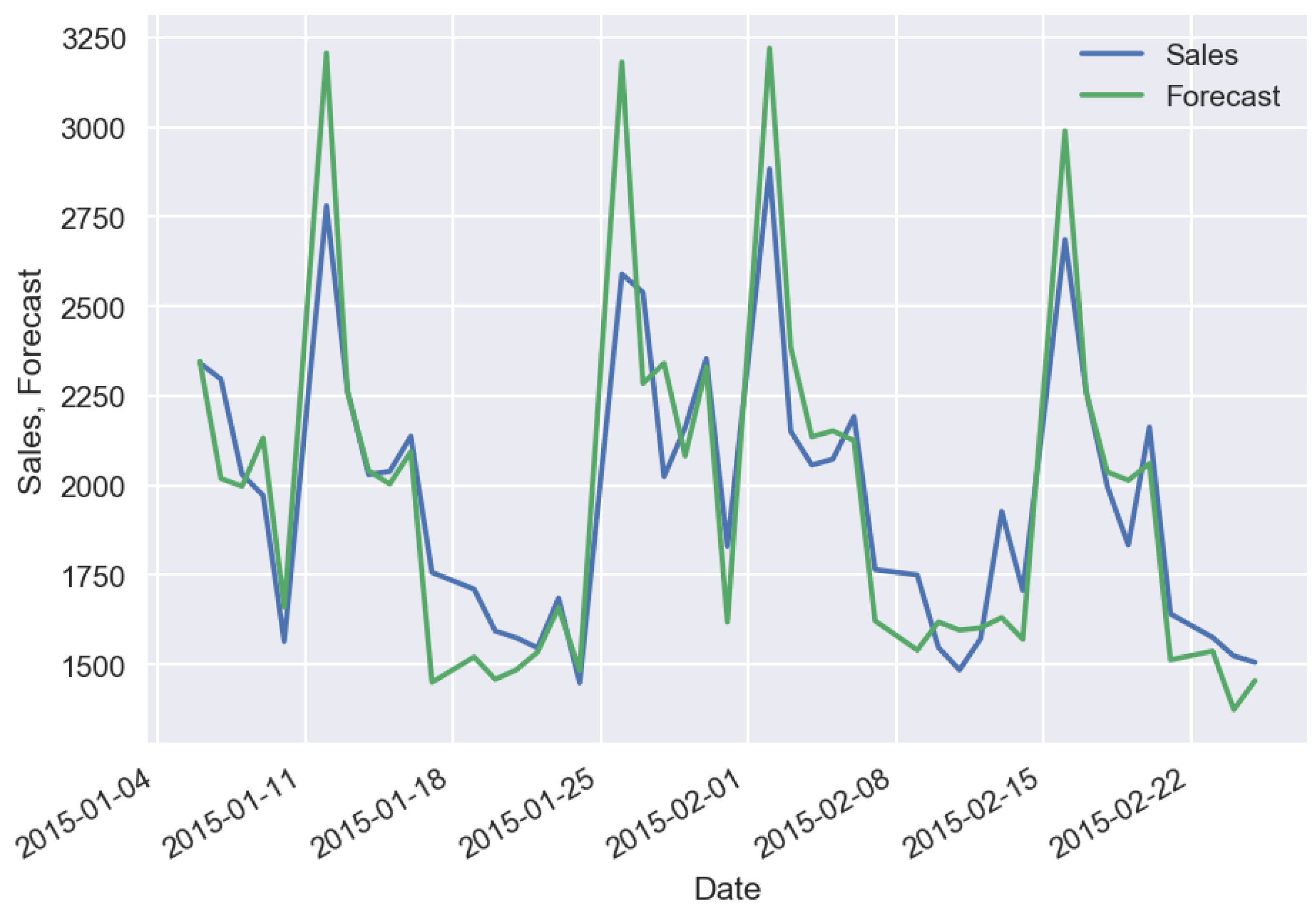
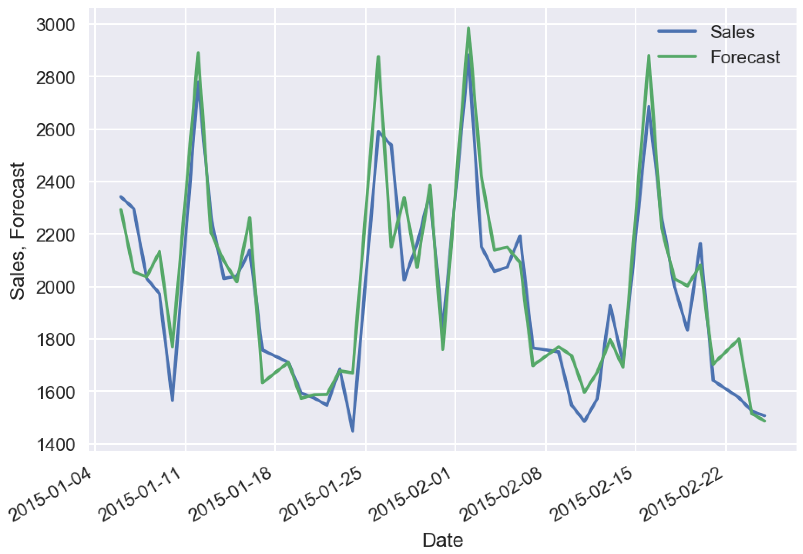
The effect of machine-learning generalization consists in the fact that a regression algorithm captures the patterns which exist in the whole set of stores or products. If the sales have expressed patterns, then generalization enables us to get more precise results which are resistant to sales noise. In the case study of machine-learning generalization, we used the following additional features regarding the previous case study: mean sales value for a specified time period of historical data, state and school holiday flags, distance from store to competitor’s store, store assortment type. Figure 10 shows the forecast in the case of historical data with a long time period (2 years) for a specific store, Figure 11 shows the forecast in the case of historical data with a short time period (3 days) for the same specific store.
In case of short time period, we can receive even more precise results. The effect of machine-learning generalization enables us to make prediction in case of very small number of historical sales data, which is important when we launch a new product or store. If we are going to predict the sales for new products, we can make expert correction by multiplying the prediction by a time dependent coefficient to take into account the transient processes, e.g., the process of product cannibalization when new products substitute other products.
4. Stacking of Machine-Learning Models
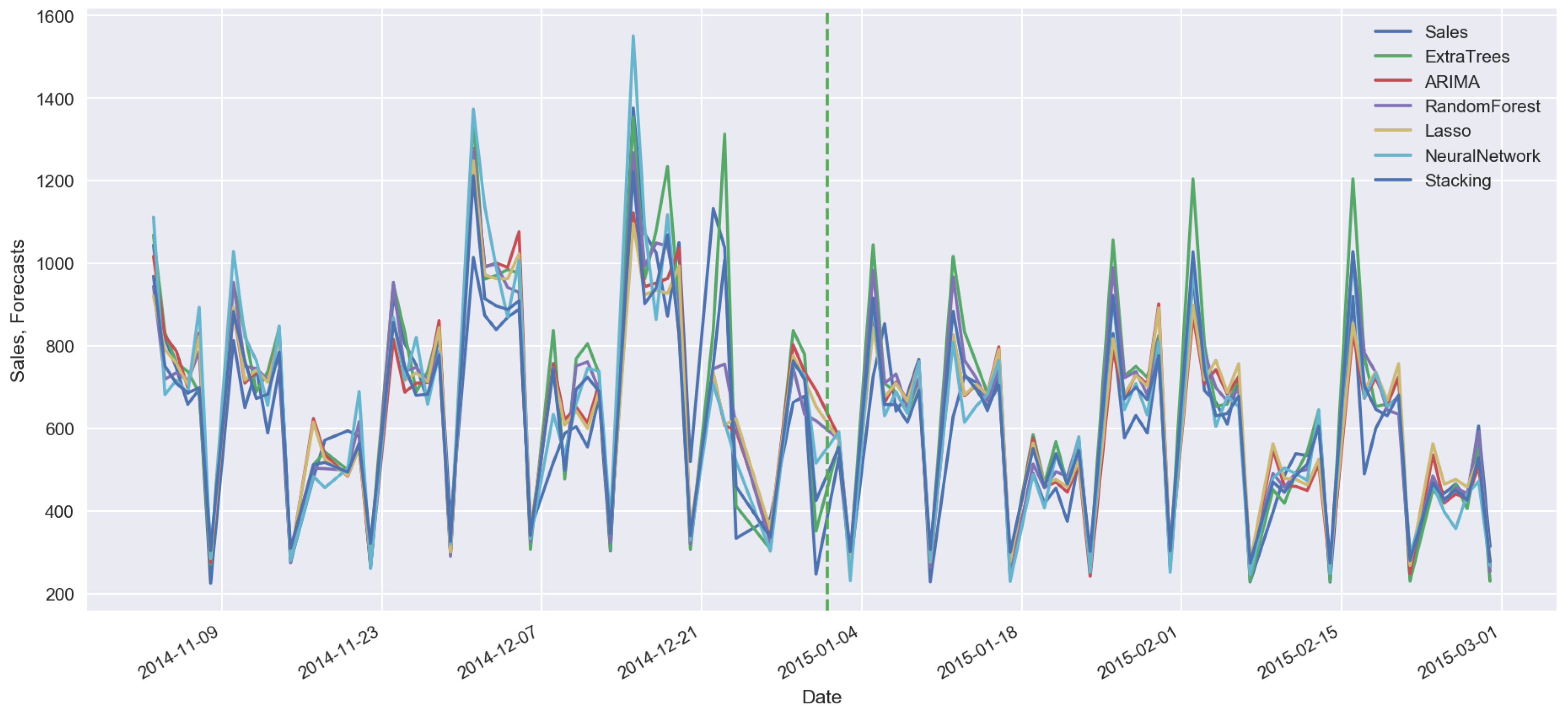
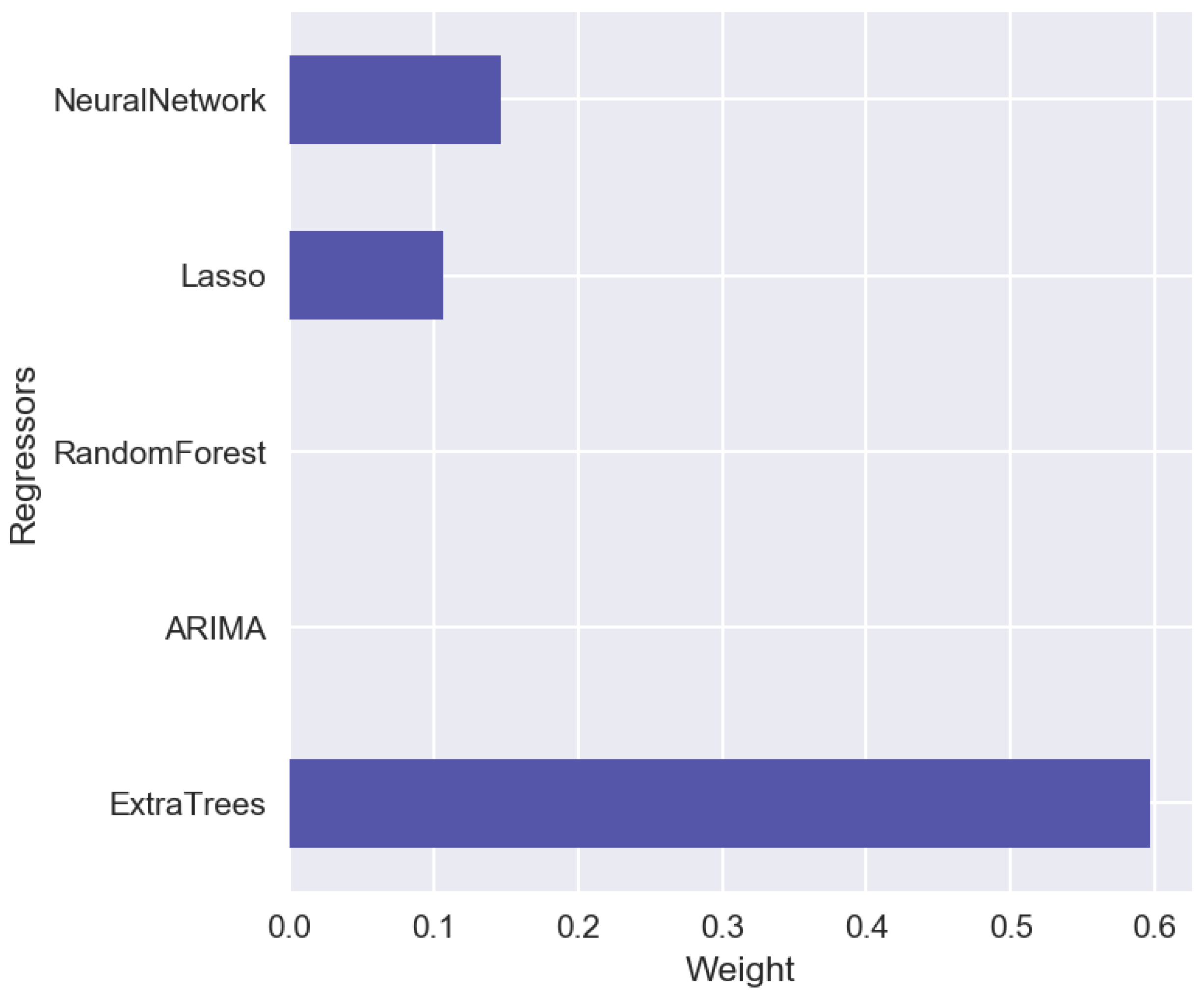
Having different predictive models with different sets of features, it is useful to combine all these results into one. Let us consider the stacking techniques [19,20,21,22,23,24] for building ensemble of predictive models. In such an approach, the results of predictions on the validation set are treated as input regressors for the next level models. As the next level model, we can consider a linear model or another type of a machine-learning algorithm, e.g., Random Forest or Neural Network. It is important to mention that in case of time series prediction, we cannot use a conventional cross validation approach, we have to split a historical data set on the training set and validation set by using period splitting, so the training data will lie in the first time period and the validation set in the next one. Figure 12 shows the time series forecasts on the validation sets obtained using different models. Vertical dotted line on the Figure 12 separates the validation set and out-of-sample set which is not used in the model training and validation processes. On the out-of-sample set, one can calculate stacking errors. hlPredictions on the validation sets are treated as regressors for the linear model with Lasso regularization. Figure 13 shows the results obtained on the second-level Lasso regression model. Only three models from the first level (ExtraTree, Lasso, Neural Network) have non-zero coefficients for their results. For other cases of sales datasets, the results can be different when the other models can play more essential role in the forecasting. Table 1 shows the errors on the validation and out-of-sample sets. These results show that stacking approach can improve accuracy on the validation and on the out-of-sample sets.
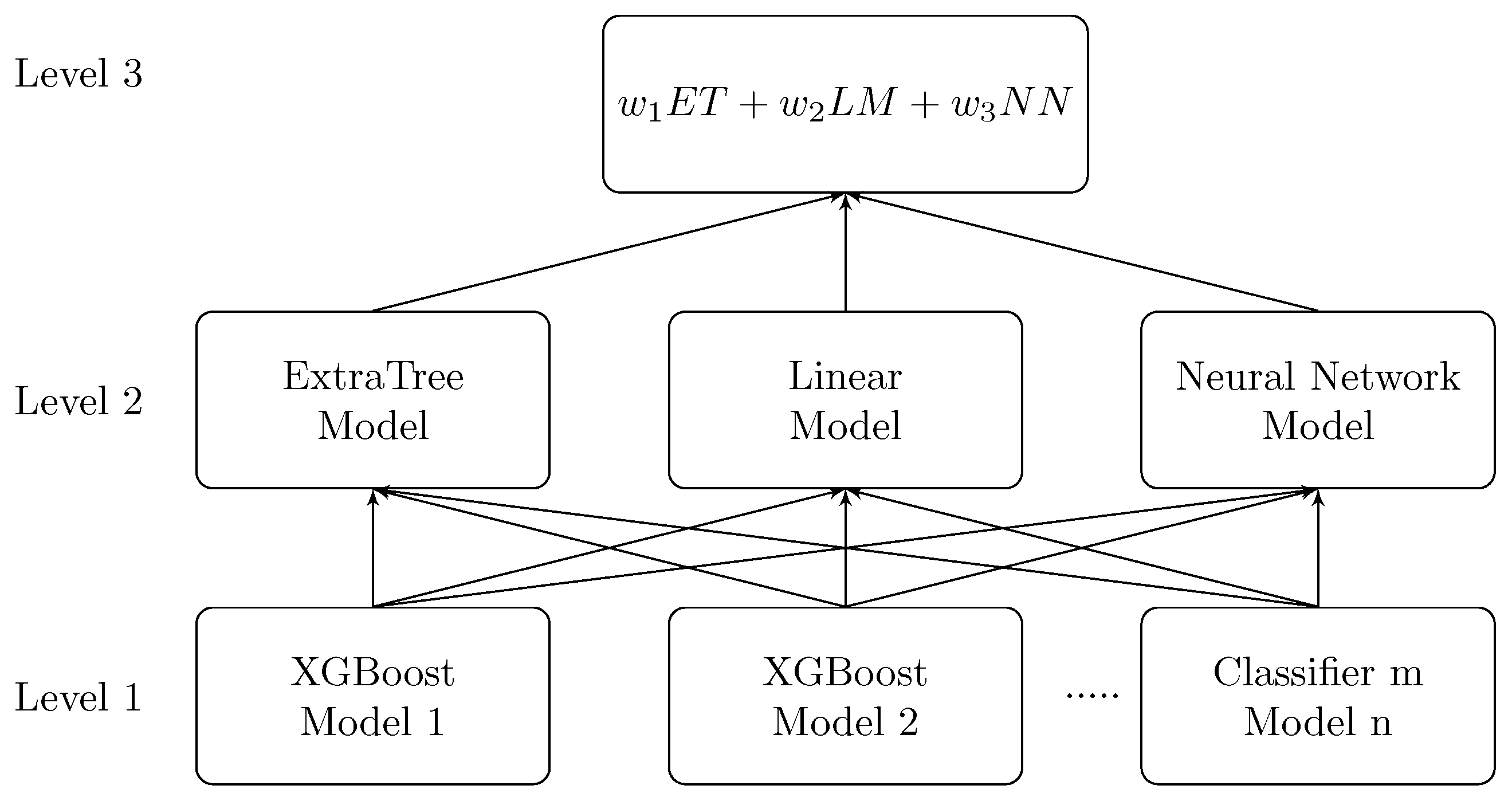
To get insights and to find new approaches, some companies propose their analytical problems for data science competitions, e.g., at Kaggle [35]. One of such competitions was Grupo Bimbo Inventory Demand [36]. The challenge of this competition was to predict inventory demand. I was a teammate of a great team ’The Slippery Appraisals’ which took the first place on this competition. The details of our winner solution are at [37]. Our solution is based on three level model (Figure 14). On the first level, we used many single models, most of them were based on XGBoost machine-learning algorithm [38]. For the second stacking level, we used two models from Python scikit-learn package—ExtraTree model and linear model from, as well as Neural Network model. The results from the second level were summed with weights on the third level. We constructed a lot of new features, the most important of them were based on aggregating target variable and its lags with grouping by different factors. More details can be found at [37]. A simple R script with single machine-learning model is at [39].
5. Conclusions
In our case study, we considered different machine-learning approaches for time series forecasting. Sales prediction is rather a regression problem than a time series problem. The use of regression approaches for sales forecasting can often give us better results compared to time series methods. One of the main assumptions of regression methods is that the patterns in the historical data will be repeated in future. The accuracy on the validation set is an important indicator for choosing an optimal number of iterations of machine-learning algorithms. The effect of machine-learning generalization consists in the fact of capturing the patterns in the whole set of data. This effect can be used to make sales prediction when there is a small number of historical data for specific sales time series in the case when a new product or store is launched. In stacking approach, the results of multiple model predictions on the validation set are treated as input regressors for the next level models. As the next level model, Lasso regression can be used. Using stacking makes it possible to take into account the differences in the results for multiple models with different sets of parameters and improve accuracy on the validation and on the out-of-sample data sets.
Funding
This research received no external funding.
Conflicts of Interest
The author declares no conflict of interest.
References
- Mentzer, J.T.; Moon, M.A. Sales Forecasting Management: A Demand Management Approach; Sage: Thousand Oaks, CA, USA, 2004. [Google Scholar]
- Efendigil, T.; Önüt, S.; Kahraman, C. A decision support system for demand forecasting with artificial neural networks and neuro-fuzzy models: A comparative analysis. Expert Syst. Appl. 2009, 36, 6697–6707. [Google Scholar] [CrossRef]
- Zhang, G.P. Neural Networks in Business Forecasting; IGI Global: Hershey, PA, USA, 2004. [Google Scholar]
- Chatfield, C. Time-Series Forecasting; Chapman and Hall/CRC: Boca Raton, FL, USA, 2000. [Google Scholar]
- Brockwell, P.J.; Davis, R.A.; Calder, M.V. Introduction to Time Series and Forecasting; Springer: Cham, Switzerland, 2002; Volume 2. [Google Scholar]
- Box, G.E.; Jenkins, G.M.; Reinsel, G.C.; Ljung, G.M. Time Series Analysis: Forecasting and Control; John Wiley & Sons: Hoboken, NJ, USA, 2015. [Google Scholar]
- Doganis, P.; Alexandridis, A.; Patrinos, P.; Sarimveis, H. Time series sales forecasting for short shelf-life food products based on artificial neural networks and evolutionary computing. J. Food Eng. 2006, 75, 196–204. [Google Scholar] [CrossRef]
- Hyndman, R.J.; Athanasopoulos, G. Forecasting: Principles and Practice; OTexts: Melbourne, Australia, 2018. [Google Scholar]
- Tsay, R.S. Analysis of Financial Time Series; John Wiley & Sons: Hoboken, NJ, USA, 2005; Volume 543. [Google Scholar]
- Wei, W.W. Time series analysis. The Oxford Handbook of Quantitative Methods in Psychology: Volume 2; Oxford University Press: Oxford, UK, 2006. [Google Scholar]
- Cerqueira, V.; Torgo, L.; Pinto, F.; Soares, C. Arbitrage of forecasting experts. Mach. Learn. 2018, 1, 1–32. [Google Scholar] [CrossRef]
- Hyndman, R.J.; Khandakar, Y. Automatic Time Series for Forecasting: The Forecast Package for R; Number 6/07; Monash University, Department of Econometrics and Business Statistics: Melbourne, Australia, 2007. [Google Scholar]
- Papacharalampous, G.A.; Tyralis, H.; Koutsoyiannis, D. Comparison of stochastic and machine learning methods for multi-step ahead forecasting of hydrological processes. J. Hydrol. 2017, 10. [Google Scholar] [CrossRef]
- Tyralis, H.; Papacharalampous, G. Variable selection in time series forecasting using random forests. Algorithms 2017, 10, 114. [Google Scholar] [CrossRef]
- Tyralis, H.; Papacharalampous, G.A. Large-scale assessment of Prophet for multi-step ahead forecasting of monthly streamflow. Adv. Geosci. 2018, 45, 147–153. [Google Scholar] [CrossRef]
- Papacharalampous, G.; Tyralis, H.; Koutsoyiannis, D. Predictability of monthly temperature and precipitation using automatic time series forecasting methods. Acta Geophys. 2018, 66, 807–831. [Google Scholar] [CrossRef]
- Taieb, S.B.; Bontempi, G.; Atiya, A.F.; Sorjamaa, A. A review and comparison of strategies for multi-step ahead time series forecasting based on the NN5 forecasting competition. Expert Syst. Appl. 2012, 39, 7067–7083. [Google Scholar] [CrossRef] [Green Version]
- Graefe, A.; Armstrong, J.S.; Jones, R.J., Jr.; Cuzán, A.G. Combining forecasts: An application to elections. Int. J. Forecast. 2014, 30, 43–54. [Google Scholar] [CrossRef]
- Wolpert, D.H. Stacked generalization. Neural Netw. 1992, 5, 241–259. [Google Scholar] [CrossRef] [Green Version]
- Rokach, L. Ensemble-based classifiers. Artif. Intell. Rev. 2010, 33, 1–39. [Google Scholar] [CrossRef]
- Sagi, O.; Rokach, L. Ensemble learning: A survey. Wiley Interdiscip. Rev. Data Min. Knowl. Discov. 2018, 8, e1249. [Google Scholar] [CrossRef]
- Gomes, H.M.; Barddal, J.P.; Enembreck, F.; Bifet, A. A survey on ensemble learning for data stream classification. ACM Comput. Surv. (CSUR) 2017, 50, 23. [Google Scholar] [CrossRef]
- Dietterich, T.G. Ensemble methods in machine learning. In Proceedings of the International Workshop on Multiple Classifier Systems, Cagliari, Italy, 21–23 June 2000; Springer: Cham, Switzerland, 2000; pp. 1–15. [Google Scholar]
- Rokach, L. Ensemble methods for classifiers. Data Mining and Knowledge Discovery Handbook; Springer: Cham, Switzerland, 2005; pp. 957–980. [Google Scholar]
- Armstrong, J.S. Combining forecasts: The end of the beginning or the beginning of the end? Int. J. Forecast. 1989, 5, 585–588. [Google Scholar] [CrossRef] [Green Version]
- Papacharalampous, G.; Tyralis, H.; Koutsoyiannis, D. Univariate time series forecasting of temperature and precipitation with a focus on machine learning algorithms: A multiple-case study from Greece. Water Resour. Manag. 2018, 32, 5207–5239. [Google Scholar] [CrossRef]
- James, G.; Witten, D.; Hastie, T.; Tibshirani, R. An Introduction to Statistical Learning; Springer: Cham, Switzerland, 2013; Volume 112. [Google Scholar]
- Breiman, L. Random forests. Mach. Learn. 2001, 45, 5–32. [Google Scholar] [CrossRef]
- Friedman, J.H. Greedy function approximation: A gradient boosting machine. Ann. Stat. 2001, 29, 1189–1232. [Google Scholar] [CrossRef]
- Friedman, J.H. Stochastic gradient boosting. Comput. Stat. Data Anal. 2002, 38, 367–378. [Google Scholar] [CrossRef] [Green Version]
- Pavlyshenko, B.M. Linear, machine learning and probabilistic approaches for time series analysis. In Proceedings of the IEEE First International Conference on Data Stream Mining & Processing (DSMP), Lviv, Ukraine, 23–27 August 2016; IEEE: Piscataway, NJ, USA, 2016; pp. 377–381. [Google Scholar] [Green Version]
- Pavlyshenko, B. Machine learning, linear and Bayesian models for logistic regression in failure detection problems. In Proceedings of the 2016 IEEE International Conference on Big Data (Big Data), Washington, DC, USA, 5–8 December 2016; IEEE: Piscataway, NJ, USA, 2016; pp. 2046–2050. [Google Scholar] [Green Version]
- Pavlyshenko, B. Using Stacking Approaches for Machine Learning Models. In Proceedings of the 2018 IEEE Second International Conference on Data Stream Mining & Processing (DSMP), Lviv, Ukraine, 21–25 August 2018; IEEE: Piscataway, NJ, USA, 2018; pp. 255–258. [Google Scholar]
- ’Rossmann Store Sales’, Kaggle.Com. Available online: http://www.kaggle.com/c/rossmann-store-sales (accessed on 3 November 2018).
- Kaggle: Your Home for Data Science. Available online: http://kaggle.com (accessed on 3 November 2018).
- Kaggle Competition ’Grupo Bimbo Inventory Demand’. Available online: https://www.kaggle.com/c/grupo-bimbo-inventory-demand (accessed on 3 November 2018).
- Kaggle Competition ’Grupo Bimbo Inventory Demand’ #1 Place Solution of The Slippery Appraisals Team. Available online: https://www.kaggle.com/c/grupo-bimbo-inventory-demand/discussion/23863 (accessed on 3 November 2018).
- Chen, T.; Guestrin, C. Xgboost: A scalable tree boosting system. In Proceedings of the 22nd ACM SIGKDD International Conference on Knowledge Discovery and Data Mining, San Francisco, CA, USA, 13–17 August 2016; ACM: New York, NY, USA, 2016; pp. 785–794. [Google Scholar]
- Kaggle Competition ’Grupo Bimbo Inventory Demand’ Bimbo XGBoost R Script LB:0.457. Available online: https://www.kaggle.com/bpavlyshenko/bimbo-xgboost-r-script-lb-0-457 (accessed on 3 November 2018).
Figure 1.
Typical time series for sales.

Figure 2.
Boxplots for sales distribution vs. day of week.

Figure 3.
Factor plots for aggregated sales.

Figure 4.
Pair plots with log(MonthSales), log(Sales), CompetitionDistance.

Figure 5.
Sales forecasting (train set error: 3.9%, validation set error: 11.6%).

Figure 6.
Feature importance.

Figure 7.
Forecast residuals for sales time series.

Figure 8.
Rolling mean of residuals.

Figure 9.
Standard deviation of forecast residuals.

Figure 10.
Sales forecasting with long time (2 year) historical data, error = 7.1%.

Figure 11.
Sales forecasting with short time (3 days), historical data, error = 5.3%.

Figure 12.
Time series forecasting on the validation sets obtained using different models.

Figure 13.
Stacking weights for regressors.

Figure 14.
Mulitilevel machine-learning model for sales time series forecasting. © 2019 IEEE. Reprinted, with permission, from Bohdan Pavlyshenko. Using Stacking Approaches for Machine Learning Models. In Proceedings of the 2018 IEEE Second International Conference on Data Stream Mining & Processing (DSMP), Lviv, Ukraine, 21–25 August 2018.


Table 1.
Forecasting errors of different models.
| Model | Validation Error | Out-of-Sample Error |
|---|---|---|
| ExtraTree | 14.6% | 13.9% |
| ARIMA | 13.8% | 11.4% |
| RandomForest | 13.6% | 11.9% |
| Lasso | 13.4% | 11.5% |
| Neural Network | 13.6% | 11.3% |
| Stacking | 12.6% | 10.2% |
© 2019 by the author. Licensee MDPI, Basel, Switzerland. This article is an open access article distributed under the terms and conditions of the Creative Commons Attribution (CC BY) license (http://creativecommons.org/licenses/by/4.0/).
Share and Cite
MDPI and ACS Style
Pavlyshenko, B.M. Machine-Learning Models for Sales Time Series Forecasting. Data 2019, 4, 15. https://0-doi-org.brum.beds.ac.uk/10.3390/data4010015
AMA Style
Pavlyshenko BM. Machine-Learning Models for Sales Time Series Forecasting. Data. 2019; 4(1):15. https://0-doi-org.brum.beds.ac.uk/10.3390/data4010015
Chicago/Turabian StylePavlyshenko, Bohdan M. 2019. "Machine-Learning Models for Sales Time Series Forecasting" Data 4, no. 1: 15. https://0-doi-org.brum.beds.ac.uk/10.3390/data4010015