Reinforcement Learning in Financial Markets


School of Computer Science, Building J12, University of Sydney, 1 Cleveland Street, Darlington, NSW 2006, Australia
*
Author to whom correspondence should be addressed.
Data 2019, 4(3), 110; https://0-doi-org.brum.beds.ac.uk/10.3390/data4030110
Submission received: 30 June 2019
/
Revised: 23 July 2019
/
Accepted: 26 July 2019
/
Published: 28 July 2019
(This article belongs to the Special Issue Data Analysis for Financial Markets)
Abstract
:Recently there has been an exponential increase in the use of artificial intelligence for trading in financial markets such as stock and forex. Reinforcement learning has become of particular interest to financial traders ever since the program AlphaGo defeated the strongest human contemporary Go board game player Lee Sedol in 2016. We systematically reviewed all recent stock/forex prediction or trading articles that used reinforcement learning as their primary machine learning method. All reviewed articles had some unrealistic assumptions such as no transaction costs, no liquidity issues and no bid or ask spread issues. Transaction costs had significant impacts on the profitability of the reinforcement learning algorithms compared with the baseline algorithms tested. Despite showing statistically significant profitability when reinforcement learning was used in comparison with baseline models in many studies, some showed no meaningful level of profitability, in particular with large changes in the price pattern between the system training and testing data. Furthermore, few performance comparisons between reinforcement learning and other sophisticated machine/deep learning models were provided. The impact of transaction costs, including the bid/ask spread on profitability has also been assessed. In conclusion, reinforcement learning in stock/forex trading is still in its early development and further research is needed to make it a reliable method in this domain.
1. Introduction
Machine learning-based prediction methods has been extensively used in medical, financial and other domains [1,2,3,4]. Buy and sell trading decisions on the financial market could be decided by either human or artificial intelligence. There has been a steady increase in the use of machines to make trading decisions on both the foreign exchange market and the stock market. Usually the training of artificial intelligence to perform financial trading involves extracting raw data as inputs and finding or recognising patterns within a training process in order to make a decision regarding the task at hand as the output. This process is called machine learning and in this context it can be used to understand rules for buying and selling and executing them. However, the scope of the systematic review is reinforcement learning. Reinforcement learning techniques are those where the system or agent are repeatedly fed new information from the available raw data in an iterative process that allows them to maximise the value of a certain pre-determined reward. It is a growing and popular method to make predictions in the financial market after the program AlphaGo defeated the strongest human contemporary Go board game player Lee Sedol in 2016. The forex market is included as it is the largest financial market by trade volume in the world.
The majority of articles considered were published in recent years due to the exponential growth in the area but older articles were considered when relevant. Each section of this review aims to cover a distinct topic within the broad field of reinforcement learning. The review articles are all grouped based on the topic titles within this review article. Finally, the review wraps everything up with a conclusion.
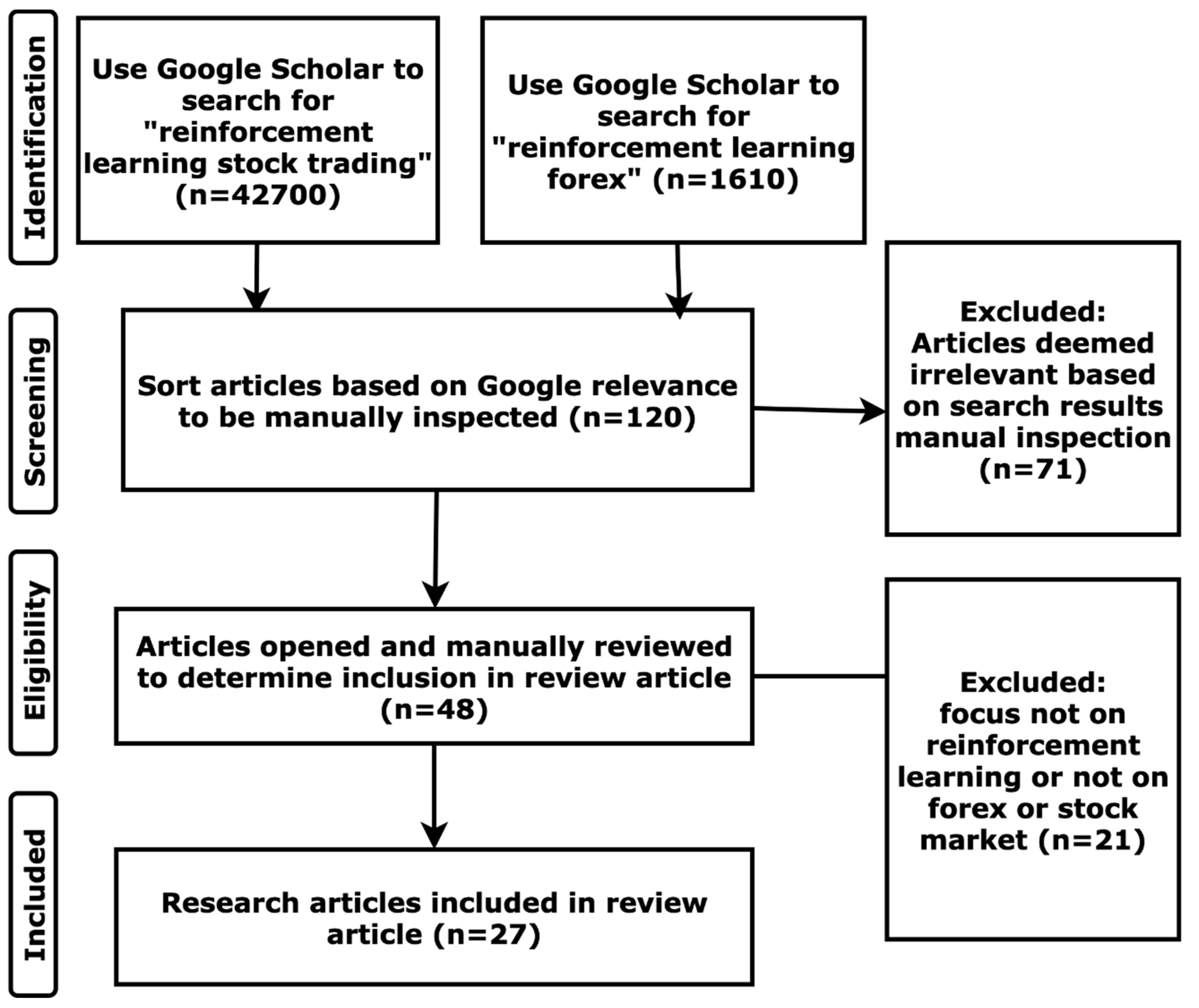
Google Scholar was used to search for the reinforcement learning articles for this systematic review. By typing into Google Scholar the key phrases “reinforcement learning forex” and “reinforcement learning stock trading” and then all the results were filtered according to the selection process given below in Figure 1. The search results returned from Google Scholar was automatically sorted by relevance, therefore only the first few pages are selected for manual inspection for eligibility. Afterwards, the results of the searched phrases were manually inspected without opening the article links to determine the most relevant articles for this systematic review. The selected articles from this step were then opened and their content read through to determine the final list of articles to be reviewed. Of 27 articles reviewed, 20 articles implemented or simulated trades to maximise profit and 7 articles were only interested in forecasting future financial asset prices. Of 20 trading articles 11 articles provided comparison with other models and 10 did not.
The overwhelming majority of the articles were focused on the forecasting in either the foreign exchange market or the stock market. However, there were several articles such as [5,6,7] that were comprehensive enough to analyse forecasting and trading on both types of markets. However, three articles by García-Galicia et al. in 2019, Pendharkar et al. in 2018 and Jangmin O et al. in 2006 were focused on the allocation of financial assets to a portfolio to maximise returns which made them the most unique articles within the 28 articles reviewed. It showed that most articles within this systematic review had a very narrow research scope that did not extend well into broad financial asset trading or management. The performance measure for all the trading algorithm articles were either the Sharpe ratio or the rate of return. The forecast only algorithms performances were measured using goodness of fit measures such as root mean squared error (RMSE). Once again, García-Galicia et al. in 2019 was unique in that instead of presenting a standard measure of rewards or results an optimal portfolio asset weight matrix was presented instead.
2. Base Reinforcement Learning
Reinforcement learning was first introduced and implemented in the financial market in 1997 [8]. Standard reinforcement learning, a type of machine learning that iteratively learned about the optimal timing of trades through new information, were used in many different contexts such as those given in Kanwar in 2019 to manage stocks and bonds in a portfolio [9] and Cummings in 2015 to manage the foreign exchange market [10].
Each article presented the methodologies in a different way. Cumming in 2015 applied the same idea using least-squares temporal difference on several different foreign exchange currency pairs such as EUR/GBP, USD/CAD, USD/CHF, USD/JPY etc [10]. Kanwar in 2019 used reinforcement learning to optimise a financial portfolio in order to maximise the return over a long period. The algorithm was model free but the parameters were learned and iteratively improved using Policy Gradient and Actor Critic Methods on real past stock market data [9]. Note in this case whenever the algorithm took an action, the net change in wealth was received as feedback in order to either reinforce or discourage the previous decision made [9].
As a result of the different methodologies the results returned from each article was different as well. The results of Cumming in 2015 had very limited success yielding only 0.839% annualised return over all currency pairs with some of the rates showing negative returns [10]. The results of the deep reinforcement learning algorithm in Kenwar in 2019 showed it was able to outperform the baseline methods described above by capturing the broad market movement pattern in some cases but in other cases the performance was very poor at 0.486 Sharpe ratio overall [9]. The results showed that deep reinforcement learning was not as successful in capturing the dynamic changes in the stock market as originally thought [9].
Each article had several advantages and disadvantages. The main advantages of Kanwar in 2019 were that the rewards generated were compared with more than the usual number of baseline models including Following the Winner, Follow the Loser and Uniformly Balanced and the change in actual amount of wealth at each iteration was used to provide precise feedback as to the future action that should be taken [9]. The main disadvantage was that although the algorithm made theoretical sense from the data, its overall performance was rather poor with only 0.486 Sharpe ratio [9]. The main advantages of Cumming in 2015 were that the algorithm results were tested on many different types of exchange rates and applied the least square temporal difference to incorporate the dependency between the exchange rates at different points in time whilst the disadvantage was that the algorithm made the extremely simplifying assumption of not considering transaction costs at all and still achieving a low level of profitability [10].
3. On and Off Policy Reinforcement Learning
Reinforcement learning can be divided into two separate categories: On policy learning and off policy learning with algorithms trained using these categories in [11,12]. They were both online policies in that they were learning new information to make decisions when they were running at the end of each step, as opposed to offline policies that only learned once the algorithm finished running at the end of the final step such as support vector machine [11]. On policy learning included SARSA (state-action-reward-state-action) that learned policies and evaluated consequences of the action currently taken [11]. Off-policy learning included Q-learning policies and would evaluate the rewards independent of the current action as they were always evaluating all the possible current actions to see which action could maximise the reward gained at the next step [11]. Both the Q-learning and SARSA methods were developed and designed to take advantage of the fact that the market was not able to adopt the new information indicated in the adaptive market hypothesis as quickly as it arrived [13].
Within the context of the project the actions of the algorithm were normally limited to the following three possible actions: buy, sell and no-action. However, each article presented the methodologies in a different way. In Pendharkar et al. in 2018 the algorithm was trained to manage a portfolio of assets consisting of a share security that mimicked the returns of the Standard and Poor’s 500 Index and a bond security that mimicked the returns of Barclays Capital Aggregate Bond Index (AGG) in the United States or the 10-year US Treasury-note [11]. Trading decisions, i.e., adjustments to the weighting of the two assets within the portfolio were made at the end of specified periods (quarter, semi-annual, annual) within the investment horizon of several decades [11]. It also showed that during the training process of the Q-learning algorithm there was a pre-determined probability that the algorithm chose an action that may not maximise the reward at the next step in order to learn what were the rewards or consequences of the action in question [11]. Marco Corazza et al. showed in 2015 it was possible to use these techniques to create algorithms that executed profitable trades with positive returns based on the adaptive market hypothesis that asserted the market prices vary over time based on the changing risk aversion of the investors and market efficiency [13]. It was conducted using several selected shares on the Italian stock market over an investment period of 30 stock market years with the algorithm making buy and sell decisions on the six selected shares over the period [13]. Deep Q-learning have also been applied to the foreign exchange market against the baseline buy and hold strategy and an expert trader [14] as well as to a stock market index [15]. Sornmayura in 2019 applied this methodology and compared its performance against the expert trade and baseline buy and hold strategy using the currency pairs EUR/USD and USD/JPY within 15 years of foreign exchange market data [14]. D’Eramo et al. in 2016 attempted to use Q-learning to predict the future movement of foreign exchange currency pairs and thus the most profitable action to take at any point in time [12]. The list of actions were given in a state space and included buying, selling or closing a position with each transaction having a fixed cost [12]. Four different types of Q-learning and learning policy were trained on a training dataset and then tested on a testing dataset [12]. They were the ε-greedy policy Q-learning, ε-greedy policy double Q-learning and weighted Q-learning as well as weighted policy for weighted Q-learning [12].
The results of the article by Sornmayura in 2019 showed the deep Q-learning algorithm had little problem significantly outperforming the baseline buy and hold strategy but it could only significantly outperform the expert trade for the EUR/USD (43.88% annualised return) and not the USD/JPY pair (26.73% annualised return) [14]. The study results warranted further study in the area [14]. D’Eramo et al. in 2016 showed the weighted policy of weighted Q-learning performed the best on the test dataset (with an annualised return of around 6%) due to the fact it was more explorative than the other policies which generally resulted in better estimation of Q-values, in particular when there was only one desirable action that was significantly more profitable than other actions [12]. Within the article by Marco Corazza et al. in 2015 the results showed that Q-learning executed more trades compared with the SARSA meaning that the SARSA method was likely to have lower overall transaction costs incurred although it may have the undesirable side effect of staying out of the market for too long [13]. The more exploratory nature of the Q-learning algorithm most likely explained why it obtained a better overall result than the SARSA method (75% of the simulations obtained positive returns under Q-learning compared with 72% of the simulations under SARSA) [13]. The results of the Pendharkar et al. in 2018 showed the cumulative profit over the 17 year test period was about 10 times the initial investment [11]. The portfolio value increased by about 10 times over the testing period of 17 years [11].
The main advantages of Pendharkar et al. in 2018 were that both the Q-learning and SARSA algorithms were applied and their results compared with one another and that the algorithm also at certain times considered an action that did not always maximise the reward to learn the reward from sometimes sub-optimal actions and the main disadvantage was that transaction costs were assumed to be non-existent which inflated the profitability of the algorithm [11]. The main advantages of Marco Corazza et al. in 2015 were that both the Q-learning and SARSA algorithms were applied and their results compared with one another and the shares whose data was used to train the algorithms were ran over a very long period of 30 years [13]. The main drawback was that only six individual shares on the Italian market were included in the training of the algorithms which meant the results were unlikely to be replicable in other financial markets [13]. The main benefits of the Sornmayura article in 2019 were that the algorithm was compared with the performance of an expert trader, something that was rarely done within trading algorithm articles and that the algorithm was trained and tested over a very long period of 15 years [14]. The advantages of the article by D’Eramo et al. in 2016 were its attempt to train, test and compare four different types of Q-learning algorithms whilst including the transaction costs in the entire process [12]. The main drawback of both articles was the lack of application of SARSA algorithms unlike the previous articles mentioned. Additionally, within the Sornmayura article in 2019 only two different foreign exchange currency rates were considered and trained in the algorithm [12,14].
4. Modifications to Reinforcement Learning
Modifications to the base reinforcement learning method described above could be implemented as well in order to achieve better results. Elder in 2008 attempted a modification of the standard reinforcement learning approach by adapting the underlying market regimes via a hierarchical learning method that continually updated the trading strategy through new observations [16]. This learning method was compared with the standard reinforcement learning agent and tested on simulated market data from the Russell 2000 Index on the New York Stock Exchange [16]. Moody et al. in 1998 attempted the use of recurrent reinforcement learning to account for dependency between current and prior inputs [8]. The idea was that due to the temporal correlation of the past share prices a reinforcement system was better at creating profitable trades than standard recurrent learning algorithms [8]. The trained algorithm was tested on the monthly Standard and Poor 500 stock index over a 25-year period from 1970 to 1994 [8]. The trading strategy was compared with the baseline buy and hold model with an assumed transaction cost of 0.5% per transaction and any profits and dividends were reinvested into the market [8]. Note this idea could be further refined into threshold recurrent reinforcement learning as shown by Maringer et al. in 2010 [17]. Li et al. in 2007 adopted two hybrid reinforcement learning systems that were called actor-only and actor-critic which were used on neural networks for stock market prediction [18]. The hybrid reinforcement learning systems were tested on two stock indices Standard & Poor’s 500 and NASDAQ Composite, as well as an individual stock IBM listed on the New York Stock Exchange [18]. The data ranged over a period of 21 years from January 1984 to June 2004 (NASDAQ started in October 1984) [18]. The 50-day training period was fixed and used to train the system for the next day prediction on a rolling basis [18]. Stone et al. in 2004 documented several different autonomous stock-trading agents with one of them being reinforcement learning [19]. The Penn Exchange Simulator (PXS), a virtual environment for stock trading that merged together virtual orders from any algorithms with real-time orders from the real stock market [19].
The results within Elder in 2008 showed that other than the trivial setup where no market observations were learned through the financial indicators used to make the trading decisions, there were no significant statistical difference in the rewards gained from using either agent [16]. The study suggested that the inconsistent nature of the reward signals or the assumptions made in the rewards function of the hierarchical reinforcement caused this result [16]. However, it was also found that the hierarchical reinforcement agent behaved like human traders by increasing the number of trades and their profitability with more market information and made less trades with increases in transaction costs [16]. In fact, the cumulative return with the transaction costs included was minus 10% [16]. The results within Moody et al. in 1998 showed that the maximisation of the differential Sharpe ratio yielded more consistent share returns than maximising profits or minimising mean squared error [8]. The resulting profits using the reinforcement system were significantly higher than the baseline buy and hold model (0.83 Sharpe ratio to 0.34 Sharpe ratio) [8]. The actor-only system performed poorly in comparison with the baseline models but the actor-critic system did outperform the baseline models including the Elman Network, showing significant short-term market predictive ability [18]. It was speculated before that the random walk may not be sufficient in incorporating the abnormal, irrational part of human psychology that helped to drive the price movements within the share market [18]. The improvement in performance by the actor-critic system (with mean absolute percentage error (MAPE) of 0.87%) in comparison with baseline neural network could be seen as evidence that the reinforcement learning system had some success in incorporating this factor into the share market prediction [18]. Stone et al. in 2004 showed the performance of the algorithm was measured by the average of the daily returns with its daily position reset before the share market closed every trading day [19]. For the reinforcement learning algorithm, the action space consisted only of a single variable that represented the volume of shares to purchase (if number is positive) or sell (if number is negative) with the price to buy and sell determined by the market at that point in time [19]. This trading strategy was then compared with other strategies tested including trend following and market making as well as the baseline static order-book imbalance strategy [19].
The advantage of all the articles in this section was that the modifications made served as a springboard to explore relatively unorthodox reinforcement learning methodologies that could improve the algorithms’ performance whilst the main disadvantage was that there were little proven history of these modifications reliability and no related articles for comparison purposes. Another advantage within the article by Elder in 2008 was that it considered the potential algorithm profitability from both the long and short positions with the main disadvantage being that there were no statistically significant returns generated from the trading algorithms [16]. Another advantage within the article by Moody in 1998 was that it considered several different trading criterion including profit/wealth, economic utility, the standard Sharpe and a modified differential Sharpe ratio that was shown to be the most effective performance measurement whilst applying several different levels of transaction costs and assessing the performance impact [8]. The main disadvantage being that the returns generated were only compared with the baseline buy and hold model which was almost never used in real life [8]. The advantage within the article by Li et al. in 2007 was that it considered different performance measures including the average daily RMSE, mean absolute deviation and mean absolute percentage error as performance criterion. It also built an Elman Network from neural networks as a baseline for prediction, a type of model comparison that was rarely conducted. The main disadvantage being that the actor-only system did not create any significant improvement in comparison with the baseline model whilst the actor-critic system only generated slight improvements [18]. Additional advantages from the article by Stone et al. in 2004 were that the PXS considered the number of shares to be traded as well as the price they were traded at and considered relatively complex baseline strategies including the Static Order-Book Imbalance strategy [19]. The disadvantage was its very poor performance (−0.82 Sharpe ratio) in comparison with both the baseline strategy and all the other strategies listed and tested in this study [19].
5. Continuous Time Unit Models
Most of the portfolio optimisation methods described above were measured using discrete time units. However, it was also possible to measure the portfolio returns using continuous time units [20]. García-Galicia et al. in 2019 used a reinforcement learning system based on an actor critic combination and created the system through the calculation of transition rates in continuous-time discrete-state Markov chain structure based portfolio problems [20]. The chain structure was characterised by probability transition rate and rewards matrices for each state derived from the observed financial assets price data and was used to determine the optimal weight for different assets in a portfolio [20]. The optimisation problem boiled down to a convex quadratic minimisation problem with linear constraints represented by Lagrange multipliers which could also represent the constraints caused by the continuous timeframe [20]. The matrix representation of the different states and their respective utilities allowed the agent to choose the course of action that maximised its utility [20]. Lee in 2001 showed that the continuous time unit within the share price movement and portfolio management could also be measured and modelled using the Markov process and the multi-layer neural network trained through reinforcement learning [21]. In this case, the states which contained the financial indicator and past price value information needed for the neural network to learn the likely future price movement almost never encountered the same values as before [21]. Note each state had different elements that incorporated all the information listed above and due to the relative subjective nature of what information should be included there could be different algorithms being trained as a result [21].
The results of the algorithms were rather different as well. The researchers García-Galicia et al. in 2019 were able to estimate the required matrices successfully to create the system but unfortunately did not provide any comparable performance measures with other trading algorithms [20]. The algorithm from Lee et al. in 2001 was trained using 2 years of past share price for 100 different shares from the South Korean stock market whilst the test data was one year of past share price for 100 different shares from the same market [21]. Different periods of future price prediction was conducted and the accuracy of the predictions were measured by the root mean squared error with an average of 3.02 over a five-day forecast period [21].
The advantage of the article by García-Galicia et al. in 2019 was that it considered a sophisticated matrix system for determining the weights of the financial assets in the investment portfolio and an utility function was used as the reward criterion rather than the more conventional criterion such as rate of return or Sharpe ratio with the main disadvantage being the simplifying assumptions that there were zero transaction costs and all investors had homogenous expectations and were risk-averse [20]. The advantages of the article by Lee in 2001 was the use of the sophisticated Markov process and the multi-layer neural network trained to improve the reinforcement learning algorithm whilst incorporating a broad group of relevant information such as the past financial indicators into the model input [21]. Another advantage was the attempt to compare the prediction results from different forecast intervals [21]. The disadvantage was that the lack of a trading system which highlighted the potentially significant gap between profitable trading and forecasting price movement accuracy as well as the poor performance when the prediction period was either too short (1 day) or too long (20 days) [21].
6. Recurrent Neural Network and Q Learning Combined
This section presents all the articles reviewed that combined recurrent neural network and Q-learning in some form. Moody et al. in 2001 presented two different trading systems based on recurrent reinforcement learning and Q-learning using neural networks with the tanh activation function [6]. These methods were applied on two separate real-life financial trading tasks [6] and were an extension on a similar study conducted in 1999 by the same researchers [7]. The first was as an intra-day currency trader on the USD/GBP foreign exchange rate data using the complete first 8 months of historical data within 1996 [6]. For this task, the trading algorithm was trained using recurrent reinforcement learning to maximise a risk-adjusted return called differential downside deviation ratio [6]. Note both the bid and ask prices were used meaning there were transaction costs. The data was then rolled forward on two-week basis for testing and generating trading signals on out-of-sample data [6]. Another experiment within the same article involved the use of 25 years of Standard & Poor’s 500 stock index from 1970 to 1994 [6]. In 1999 the researchers found that when testing on the Standard & Poor’s 500/Treasury Bill allocation problem the standard Q-learning method was inferior to the recurrent reinforcement learning system [7]. Therefore in 2001 the researchers used the advantage updating refinement Q-learning in lieu of the standard Q-learning method [6]. Pendharkar et al. in 2018 had shown the presence of complex neural networks did allow the required pattern generalisation power, including to non-linear relationships, that was very much needed in the financial market to make profitable trades [11]. Ha Young Kim et al. in 2018 combined the Q-learning algorithm with the deep neural network, meaning neural network with many different hidden layers of neurons between the input (raw data in the financial market) and output action [22]. The number of shares to be traded (for a given level of existing capital) was determined using the decisions made by the deep neural network, something that was often neglected or set to a default value when constructing stock or other financial asset trading algorithms [22]. It also adopted various action strategies that used Q-values to analyse profitable actions within a confused market, defined as a financial market with no clear direction or movement [22]. Another adoption of Q-learning algorithm with neural networks was completed by Carapuço et al. in 2018 [23]. Three hidden layers were used in the neural networks trained under the Q-learning algorithm with the Rectified Linear Unit as the activation function [23].
Moody et al. in 2001 showed that over the six month test period for the USD/GBP exchange rate, the recurrent reinforcement learning trading system achieved a 15% return and a Sharpe ratio of 2.3 after annualization [6]. Both the long and short position could be maintained with any unused funds invested in three-month Treasury Bills and a 0.5% transaction cost was included in the calculation of profits with the assumption that any profits earned were reinvested into the stock market during trading [6]. The recurrent reinforcement learning was compared with the Q-learning algorithm [6]. The returns of the recurrent reinforced learning method over dozens of different trials were still significantly better than that of the Q-learning method (Sharpe ratio of 0.83 versus 0.63) and both of them outperformed the baseline buy and hold method by a considerable margin [6]. Within Pendharkar et al. in 2018 during the period of market confusion the trained results from the market data was not very helpful and thus a pre-determined action was triggered once market condition exceeded a pre-determined threshold measured by market price movement [22]. This usually resulted in delays to buy or sell until a more profitable time as the most profitable strategy [22]. This method outperformed the standard method of buying and selling a fixed number of shares on various stock market indices such as the Standard & Poor’s 500, Korea Composite Stock Price Index (in South Korea), Hang Seng Index (in Hong Kong) and EUROSTOXX50 [22]. The overall profit on the Standard & Poor’s 500 index was increased by 4.5 times compared with the baseline reinforcement model [22]. The adoption of the Q-learning algorithm by Carapuço et al. in 2018 eventually was able to make profitable trades based on out-of-sample data despite the difficulties presented by the lack of data predictability within the simulated foreign exchange market [23]. The algorithm was tested on the EUR/USD foreign exchange market over a period of 8 years of data from 2010 to 2017 using 10 tests of different initial conditions with an overall yearly average profit of over 15% [23]. It also appeared that the learning rate in the training dataset was stable and the model could be used for profitable trading [23].
Each article had various benefits and drawbacks. The advantages of the article by Moody et al. in 2001 were that it applied a relatively complex trading methodology on both the stock and foreign exchange market. It also incorporated different bid and ask prices into the trades as well as examined the various levels’ impact on profitability [6]. The disadvantages were that only one foreign exchange currency pair and one stock market was used for the training of the algorithm and the stock market performed mediocrely as measured by the Sharpe ratio [6]. In addition, the currency pair USD/GBP was only trained over eight months in 1996 meaning the trained algorithm was unlikely to generalise well to trading in other currency pairs especially as the rate the time period was almost flat at around 0.65 [6]. The article by Ha Young Kim et al. in 2018 had a number of advantages including the consideration of the number of shares to be traded at any time as well as the price traded at and attempted to specifically consider possible actions to take during a confused market, something encountered often in real-life trading [22]. The main disadvantage was the results were only compared with the Standard & Poor’s 500 index which did not offer a great deal of insight [22]. The advantages within the article by Carapuço et al. in 2018 were its training of the three hidden layers neural network for share trading and the testing of different initial conditions to obtain a high level of overall profitability [23]. The disadvantage was that only one foreign exchange currency pair, EUR/USD was tested over a relatively short time span of 8 years and the model performance could be measured by more sophisticated measures than the profitability on a fixed validation dataset [23].
7. Deep Neural Network and Recurrent Reinforcement Learning
Tan et al. in 2011 proposed an artificial intelligence model that employed a system called the adaptive network fuzzy inference system for technical analysis supplemented by the use of reinforcement learning [24]. In this case, reinforcement learning was used to provide useful information for the algorithm to learn including the past moving average prices and momentum period also known as the rate of change of the stock price over a period of time [24]. Random exploration of data for improvements within the algorithm was mitigated by the provision of more feedback signals. The algorithm was tested on five individual listed shares on the New York Stock Exchange which were then compared with the market indices of the Standard and Poor 500 and Dow Jones index [24]. A transaction cost of 0.5% was included for every trade within the calculation of the stock returns [24]. Lu in 2017 applied the recurrent reinforcement learning combined with deep neural network and Long Short Term Memory network (LSTM) to the foreign exchange market [25]. Note long short term memory network is a special type of recurrent neural network more capable of learning long term dependencies than standard recurrent neural networks. Huang et al. in 2018 utilised a Markov decision process model that was solved using deep recurrent Q-network and sample a longer sequence for recurrent neural network learning [26]. It could be used to train the algorithm every few steps instead of at the end of the process [26]. It included extra feedback to the agent to eliminate the need for random exploration during reinforcement learning [26]. However, this technique was only applicable to financial trading under a few market assumptions including the cost of any transaction was a fixed percentage of the value of foreign exchange currency traded [26]. It also required increases in sequence sampling for recurrent neural network training which reduced the time interval required for training the algorithm [26]. The log of daily returns was defined as the reward function [26].
The result of the proposed trading system within Tan et al. in 2011 was able to exceed the market index returns by about 50 percentage points over a period of 13 years from 1994 to 2006 [24]. The algorithm in Huang et al. in 2018 was tested on 12 different commonly traded currency pairs including GBP/USD, EUR/USD and EUR/GBP and performance was measured by common indicators such as the annualised rate of return and Sharpe ratios [26]. Positive results were achieved under the majority of the currency pairs simulations [26]. The overall result was 26.3% return using the 0.1% transaction cost assumption over all currencies tested [26].
The advantages offered by related research Tan et al. in 2011 was that it were a unique system that incorporated a wide range of information including momentum period into the algorithm and considered transaction costs as well [24]. The downside was that the algorithm was very specialised and only tested on five individual listed shares on the New York Stock Exchange [24]. The advantages within the article by Huang et al. in 2018 included its utilisation of deep recurrent neural network with Q-learning which was then tested on 12 different commonly traded currency pairs [26]. Another advantage was the interesting but worthwhile investigative result that a larger transaction spread generated better returns suggesting this was likely due to the constraint imposed by the system that forced the algorithm to look for more creative ways to profitably trade on the market [26]. A major disadvantage was the short time period for all currency pairs over the same period of time between 2012 and 2017 which diluted the advantages of using multiple currencies [26].
8. Advanced Learning Strategies in Reinforcement Learning
Reinforcement learning could be generalised into behavioural learning method that used a similar strategy for the predictions. This was tried and tested by Ertugrul et al. in 2017 where a generalised behaviour learning method (GBLM) was used to detect hidden patterns with different stock and forex indicators. The GBLM was trained using extreme learning machine similar to standard artificial neural networks [5]. Reinforcement learning could also be used as a subsequent step to genetic algorithm for forecasting of foreign exchange rates [27]. Hryshko et al. in 2004 initially used a genetic algorithm for in-sample trading strategy search to select the optimal trading strategy of entry and exit rules [27]. The data, namely the financial indicators making up the rules were then passed on to the reinforcement learning, Q-learning algorithm engine [27]. The algorithm could then be used online to continually search for the optimal strategy through repetitive experience [27]. Jangmin O et al. in 2006 presented an asset allocation strategy called meta policy that aimed to dynamically adjust the asset allocation in a portfolio to maximise the portfolio returns [28]. Reinforcement learning could also be combined with standard share market return technical graphs and indicators such as the Japanese candlesticks like those used by Gabrielsson et al. in 2015 [29]. Recurrent reinforcement learning could also be refined through parameter updates for inter-day trading and consequent higher autocorrelation between the adjacent price data within the time series of data with Zhang et al. in 2014 presented two different types of parameter updates: average elitist and multiple elitist [30]. This was a deeper analysis of the results obtained using a similar elitist methodology in 2013 by Zhang et al. with the features to be selected using genetic algorithm [31]. Zhang et al. in 2013 applied elitist recurrent reinforcement learning after using genetic algorithms to select the input features data to be included in the algorithm [31].
Several of the articles’ methodologies require a more detailed explanation than given in this section. Within Jangmin O et al. in 2006 the meta policy and any strategies were constructed within the reinforcement learning framework which utilised recommendations of local traders as well as the stock fund ratio over the asset [28]. The expert traders advice were utilised to learn the share price patterns in a supervised way [28]. The Q-learning reinforcement learning framework incorporated a relatively compact environment and the learning agent design [28]. The baseline model used were fixed asset allocation strategies compared with the dynamic asset allocation strategy tested on the Korea Composite Stock Price Index [28]. Gabrielsson et al. in 2015 attempted to combine recurrent reinforcement learning with lagged time series information from Japanese candlesticks in short, one minute intervals to create a trading algorithm using data from the Standard and Poor 500 index futures market [29]. The daily trading returns over the 31-trading-day period and Sharpe ratio were used as the performance benchmarks [29]. In Zhang et al. in 2014 the first idea, also called the average elitist method, was aimed to improve the returns on out-of-sample testing data [30]. The second idea, also called the multiple elitist, attempted to incorporate the serial correlation between the stocks within their price movements [30].
The results of each article varied considerably as well. Within the article by Ertugrul et al. in 2017 the model was trained and tested for future prediction on different stock indices and foreign exchange indices using previous values [5]. The results were compared with the artificial neural network method and showed that GBLM with a 3-month stock index MAPE (with a value of 4.82) was more successful in tracking the data trend despite the presence of natural fluctuations [5]. In Hryshko et al. in 2004 the hybrid system was tested using available past foreign exchange data with a reasonable level of gain of 6% annualised return during the test data period [27]. Within the article by Jangmin O et al. in 2006 the data from 1998 to 2001 Korea Composite Stock Price Index inclusive were used for training the algorithm whilst the subsequent two years of data was used for testing with the baseline models [28]. The results showed that over the prescribed test period, the meta policy trading strategy produced a return of around 258% that was more than twice the profits generated by the baseline fixed asset allocation strategies [28]. The algorithm from Gabrielsson et al. in 2015 was compared with three different benchmark models including a buy-and-hold model, a zero intelligence model and a basic recurrent reinforcement learning model under two separate settings: one with no trading costs and one with trading costs included [29]. The candlestick-based reinforcement learning algorithm significantly outperformed the benchmark models when transaction costs were non-existent but was not able to repeat the feat when transaction costs were included with an average overall return of 0 [29]. Within Zhang et al. in 2014 the data used to test the trading system were stocks on the Standard and Poor 500 index over the four-year period of 2009 to 2012 [30]. When the performance was measured in Sharpe ratio, the average elitist updated parameter schemes (Sharpe ratio 0.041) seemed to outperform at a statistically significant level both the multiple elitist scheme (Sharpe ratio 0.028) and the two base models strategies random trading and buy-and-hold [30]. Within Zhang et al. in 2013 the four years of data from 2009 to 2012 were split into the training, evaluation and trading set [31]. It resulted in an average Sharpe ratio of around 1 using the average results of all 500 NASDAQ company share prices tested [31].
Each article had various benefits and deficiencies. Advantages of the article by Ertugrul et al. in 2017 were the GBLM’s application on different stock and foreign exchange indices as well as the inclusion of performance comparison with artificial neural network. The disadvantage was the lack of consideration of the transaction costs [27]. The main strengths of the article by Hryshko et al. in 2004 were its inclusion of financial indicators and moving averages that made up the rules and the resulting reasonable level of profitability despite the inclusion of transaction costs [27]. The main deficiency was that the algorithm was only trained and tested on a single currency pair EUR/USD over a period of seven months from June to December 2002 at 5 min frequency base within a relatively flat trend [27]. This meant the trained algorithm was unlikely to generalise well to trading in other currency pairs. The article by Jangmin O et al. in 2006 had the additional advantages of using a relatively complex fixed asset allocation strategy as the baseline strategy with the additional disadvantage being that it used a very old Stock Price Index from 1998 to 2001 that was most likely outdated [28]. The article by Gabrielsson et al. in 2015 had the additional benefits of using three different benchmark models for comparison as well as analysing the profitability with and without transaction costs [29]. An additional strength was the zero overall rate of return once transaction costs were included [29]. The article by Zhang et al. in 2014 had the additional advantage of incorporating transaction costs into both methodologies attempted. There were the additional shortcomings of training the algorithm over a very limited time period of 4 years over a single share market index, with relatively poor returns as measured by Sharpe ratio for both methodologies [30]. The main advantage of the article by Zhang et al. in 2013 was the results from using different input features to the recurrent reinforcement learning were tried and tested with the main drawback being the assumption that the results of all 500 companies on the NASDAQ contributed equally to the final result and no transaction costs were included in the Sharpe ratio calculations [31]. The contributions of all the articles in this section were that the modifications made served as a springboard to explore relatively unorthodox reinforcement learning methodologies that could improve the algorithms’ performance whilst the main disadvantage was the little proven history of these modifications reliability and no related articles for comparison purposes.
Table 1 below gives a summary of each article reviewed.
9. Overall Analysis
Almost all trading systems reviewed made the assumptions there were no liquidity issues and no bid or ask spread incurred within the trades, which were not realistic assumptions in real-life trading especially for individual traders. In particular, few articles even mentioned this issue at all with Moody et al. in 2001 and Hryshko in 2004 being the exceptions let alone incorporated this constraint into the algorithm training and testing. This issue could be potentially resolved through the use of additional model constraints that imitated the conditions faced by an individual investor in the market.
Transaction costs, including bid/ask spreads, had significant impacts on the profitability of the reinforcement learning algorithms compared with the baseline algorithms tested. This was because these reinforcement learning algorithms usually made a relatively large number of trades within a short period of time meaning the transaction costs assumptions could play a significant role in the overall profitability of the system. This could be seen by the fact that under many of the studies such as that in and [29], an increase in transaction costs changed the profitability of the reinforcement learning system from profitable to not profitable in one stroke.
However, as the articles had little coverage of other advanced models used for financial market trading and prediction, there were little results for comparison despite being a potentially very relevant and important question. It meant this was an interesting and worthwhile future direction for these studies.
The majority of research articles were primarily focused on the price of any buy or sell orders on the market. There was far less interest in the monetary size of each trade relative to the capital available. In fact, many articles such as [6,8] made the simplifying assumption that every buy and sell order were of the same monetary size. However, in real life trading the size of these trades could have just as big an impact on the overall profitability of the trades and only a few articles such as [19,22] were interested in investigating this factor on profitability.
10. Conclusion and Future Directions
Reinforcement learning is a broad and growing field of interest within the trading of financial assets on the stock and foreign exchange market. All reinforcement papers reviewed here had settings and assumptions such as those regarding transaction costs (including bid/ask spreads), forecast periods, criterion for success that were strikingly different meaning direct comparison between their results and systems was not feasible.
From the review of the articles here it can be seen that when the reinforcement learning methodology was applied in a suitable context it could substantially improve on the performance over baseline models when the performance was based on either forecasting accuracy or trading profitability. However, there were some studies that showed reinforcement learning performed rather poorly when there were large changes in the price pattern between data used to train the system and that were used to test the system. Furthermore, performance comparison between reinforcement learning models and other models such as Autoregressive Integrated Moving Average (ARIMA), deep neural network, recurrent neural network and state space were very rare. Therefore, any definitive comparisons between them could not be drawn. For anyone interested in the field it meant reinforcement learning should be used with caution in making predictions and trades on the financial markets compared with the current artificial intelligence methods available. Any future research on reinforcement learning should focus on the possibility of comparing reinforcement learning techniques with other sophisticated models used for forecasting or trading on the financial market.
Over the past few years, reinforcement learning within the foreign exchange and financial market have been gradually dominated by the use of reinforcement learning in conjunction with other predictive models such as neural networks. The rewards of the algorithms tested in these studies are mostly the traditional Sharpe ratio or rate of returns based on historical testing data. Future possible areas of research or direction could include the following:
- –
- Testing of reinforcement learning algorithms on live trading platforms rather than just performance on historical data which would include work on setting up an operational environment for the algorithms.
- –
- More comparison of different reinforcement learning algorithms constructed and compared under similar conditions and data sources.
- –
- More comparison of reinforcement learning algorithms constructed and compared under similar conditions and data sources with other complex learning methodologies such as neural networks.
- –
- Assessment of algorithm users that encounters liquidity issues when trading compared with the default assumption of no liquidity issues.
Author Contributions
Conceptualization, T.L.M. and M.K.; methodology, T.L.M. and M.K.; investigation, T.L.M.; writing—original draft preparation, T.L.M.; writing—review and editing, T.L.M. and M.K.; supervision, M.K.
Funding
This research received no external funding.
Acknowledgments
Authors thank Melissa Tan for proof-reading and her helpful feedback.
Conflicts of Interest
The authors declare no conflict of interest.
References
- Khushi, M.; Dean, I.M.; Teber, E.T.; Chircop, M.; Arthur, J.W.; Flores-Rodriguez, N. Automated classification and characterization of the mitotic spindle following knockdown of a mitosis-related protein. BMC Bioinform. 2017, 18, 566. [Google Scholar] [CrossRef] [PubMed]
- Criminisi, A.; Shotton, J.; Konukoglu, E. Decision forests: A unified framework for classification, regression, density estimation, manifold learning and semi-supervised learning. Found. Trends® Comput. Graph. Vis. 2012, 7, 81–227. [Google Scholar] [CrossRef]
- Khalid, S.; Khalil, T.; Nasreen, S. A survey of feature selection and feature extraction techniques in machine learning. In Proceedings of the 2014 Science and Information Conference, Warsaw, Poland, 7–10 September 2014; pp. 372–378. [Google Scholar]
- Khushi, M.; Choudhury, N.; Arthur, J.W.; Clarke, C.L.; Graham, J.D. Predicting Functional Interactions Among DNA-Binding Proteins. In 25th International Conference on Neural Information Processing; Springer: Cham, Switzerland, 2018; pp. 70–80. [Google Scholar]
- Ertuğrul, Ö.F.; Tağluk, M.E. Forecasting financial indicators by generalized behavioral learning method. Soft Comput. 2018, 22, 8259–8272. [Google Scholar] [CrossRef]
- John Moody, M.S. Learning to Trade via Direct Reinforcement. IEEE Trans. Neural Netw. 2001, 12, 875–889. [Google Scholar] [CrossRef] [PubMed]
- Saffell, J.M. Reinforcement Learning for Trading. In Advances in Neural Information Processing Systems 11; MIT Press: Cambridge, MA, USA, 1999. [Google Scholar]
- Moody, J.; Wu, L.; Liao, Y.; Saffell, M. Performance functions and reinforcement learning for trading systems and portfolios. J. Forecast. 1998, 17, 441–470. [Google Scholar] [CrossRef]
- Kanwar, N. Deep Reinforcement Learning-Based Portfolio Management; The University of Texas at Arlington: Arlington, TX, USA, 2019. [Google Scholar]
- Cumming, J. An Investigation into the Use of Reinforcement Learning Techniques within the Algorithmic Trading Domain; Imperial College London: London, UK, 2015. [Google Scholar]
- Pendharkar, P.C.; Cusatis, P. Trading financial indices with reinforcement learning agents. Expert Syst. Appl. 2018, 103, 1–13. [Google Scholar] [CrossRef]
- D’Eramo, C.; Restelli, M.; Nuara, A. Estimating the Maximum Expected Value through Gaussian Approximation. Int. Conf. Mach. Learn. 2016, 48, 1032–1040. [Google Scholar]
- Marco Corazza, A.S. Q-Learning and SARSA: A comparison between two intelligent stochastic control approaches for financial trading. Univ. Ca’ Foscari Venice Dept. Econ. Res. Pap. 2015, 15, 1–23. [Google Scholar]
- Sornmayura, S. Robust forex trading with deep q network (dqn). Assumpt. Bus. Adm. Coll. 2019, 39, 15–33. [Google Scholar]
- Lee, J.W.; Park, J.; O, J.; Lee, J.; Hong, E. A Multiagent Approach to Q-Learning for Daily Stock Trading. IEEE Trans. Syst. ManCybern. -Part A Syst. Hum. 2007, 37, 864–877. [Google Scholar]
- Elder, T. Creating Algorithmic Traders with Hierarchical Reinforcement Learning; University of Edinburgh: Edinburgh, UK, 2008. [Google Scholar]
- Dietmar Maringer, T.R. Threshold Recurrent Reinforcement Learning Model for Automated Trading; Springer: Istanbul, Turkey, 2010. [Google Scholar]
- Li, H.; Dagli, C.H.; Enke, D. Short-term Stock Market Timing Prediction under Reinforcement Learning Schemes. In Proceedings of the 2007 IEEE International Symposium on Approximate Dynamic Programming and Reinforcement Learning, Honolulu, HI, USA, 1–5 April 2007. [Google Scholar]
- Sherstov, A.A.; Stone, P. Three automated stock-trading agents: A comparative study. In Agent-Mediated Electronic Commerce VI; Faratin, P., Ed.; Springer: Berlin, Germany, 2004. [Google Scholar]
- García-Galicia, M.; Carsteanu, A.A.; Clempner, J.B. Continuous-time reinforcement learning approach for portfolio management with time penalization. Elsevier Expert Syst. Appl. 2019, 129, 27–36. [Google Scholar] [CrossRef]
- Lee, J.W. Stock price prediction using reinforcement learning. In Proceedings of the 2001 IEEE International Symposium on Industrial Electronics, Pusan, Korea, 12–16 June 2001. [Google Scholar]
- Jeong, G.; Kim, H.Y. Improving financial trading decisions using deep Q-learning: Predicting the number of shares, action strategies, and transfer learning. Expert Syst. Appl. 2018, 117, 125–138. [Google Scholar] [CrossRef]
- Carapuço, J.; Neves, R.; Horta, N. Reinforcement learning applied to Forex trading. Appl. Soft Comput. 2018, 73, 783–794. [Google Scholar] [CrossRef]
- Tan, Z.; Philip, C.Q.; Cheng, Y.K. Stock trading with cycles: A financial application of ANFIS and reinforcement learning. Expert Syst. Appl. 2011, 38, 4741–4755. [Google Scholar] [CrossRef]
- Lu, D.W. Agent Inspired Trading Using Recurrent Reinforcement Learning and LSTM Neural Networks. Arxiv Quant. Financ. arXiv 2017, arXiv:1707.07338. [Google Scholar]
- Huang, C.-Y. Financial Trading as a Game: A Deep Reinforcement Learning Approach. Arxiv Quant. Financ. arXiv 2018, arXiv:1807.02787. [Google Scholar]
- Hryshko, A.; Downs, T. System for foreign exchange trading using genetic algorithms and reinforcement learning. Int. J. Syst. Sci. 2004, 35, 763–774. [Google Scholar] [CrossRef]
- O, J.; Lee, J.; Lee, J.W.; Zhang, B.T. Adaptive stock trading with dynamic asset allocation using reinforcement learning. Inf. Sci. 2006, 176, 2121–2147. [Google Scholar]
- Gabrielsson, P.; Johansson, U. High-Frequency Equity Index Futures Trading Using Recurrent Reinforcement Learning with Candlesticks. In Proceedings of the 2015 IEEE Symposium Series on Computational Intelligence, Cape Town, South Africa, 7–10 December 2015. [Google Scholar]
- Zhang, J.; Maringer, D. Two Parameter Update Schemes for Recurrent Reinforcement Learning. In Proceedings of the 2014 IEEE Congress on Evolutionary Computation, Beijing, China, 20 January 2014. [Google Scholar]
- Zhang, J.; Maringer, D. Indicator selection for daily equity trading with recurrent reinforcement learning. In Proceedings of the 15th annual conference companion on Genetic and evolutionary computation, Amsterdam, The Netherlands, 6–10 July 2013; pp. 1757–1758. [Google Scholar]
Figure 1.
Flowchart showing the filtering of reinforcement articles chosen for review.


Table 1.
Summary of article reviewed.
| Article | Main Goal | Market | Input Variables | Main Techniques | Transaction Cost Included | Results | Trading System |
|---|---|---|---|---|---|---|---|
| [11] | Trading | Stock | Past historical returns | Reinforcement learning on-policy and off-policy | No | 10 times increase in portfolio over 17 years | Yes |
| [13] | Trading | Stock | Past historical data | Reinforcement Learning Q learning SARSA | Yes | 75% simulations net positive return Q-learning 72% simulations net positive return SARSA | Yes |
| [22] | Trading | Stock | Past historical data | deep Q-learning (reinforcement learning) Deep neural network | No | 4.5 times higher profit compared with baseline RL model | Yes |
| [23] | Trading | Forex | Past historical data | Reinforcement learning Neural networks under Q-learning algorithm | No | Yearly average test profit 15.6 ± 2.5 | Yes |
| [26] | Trading | Forex | Past historical data | Reinforcement learning recurrent neural network training | Yes | 26.3 annualised return | No |
| [20] | Trading | Portfolio management | Past historical data | Reinforcement learning (continuous) Markov chains | Yes | No return/error. Optimal portfolio matrix. | Yes |
| [10] | Trading | Forex | Past historical data as candlesticks | Reinforcement learning LSTD, LSPI | No | 0.839% annualised return over all currency pairs | Yes |
| [14] | Forecasting | Forex | Past historical data | Reinforcement learning Deep Q-learning | No | 26.73% annualised return on USD/JPY | Yes |
| [12] | Trading | Forex | Past historical data | Multiple Q-learning | Yes | 6% return on W Q-Learning with W-policy | No |
| [5] | Forecasting | Forex/Stock | Past historical data, economic indicators | Generalised Behaviour Learning Method | No | 4.82 3 month stock index MAPE | No |
| [27] | Trading | Forex | Past historical data | Genetic Algorithms Reinforcement learning | Yes | 6% annualised return | Yes |
| [29] | Trading | Stock | Technical indicators Past historical data | Recurrent reinforcement learning | Yes | Average return of 0 | Yes |
| [30] | Trading | Stock | Past historical data Correlation coefficient | Recurrent reinforcement learning | Yes | Elitist: 0.028 Sharpe ratio Average Elitist: 0041 Sharpe ratio | Yes |
| [17] | Trading | Stock | Past historical data | Threshold recurrent reinforcement learning | Yes | Average Sharpe ratio 0.1 | Yes |
| [15] | Trading | Stock | Past historical data | deep Q-learning (reinforcement learning) Deep neural network | Yes | 4.5 times higher profit compared with baseline RL model | Yes |
| [25] | Trading | Forex | Past historical data | Recurrent reinforcement learning LSTM | Yes | Average Sharpe ratio 0.1 at 600 epochs | Yes |
| [31] | Trading | Stock | Past historical data Correlation coefficient | Recurrent reinforcement learning, Genetic Algorithms | No | Elitist: 1 Sharpe ratio on average | Yes |
| [9] | Trading | Stock | Past historical data Volume | Deep Reinforcement Learning | Yes | 0.486 Sharpe ratio | Yes |
| [16] | Trading | Stock | Real historical data for simulation | Hierarchical reinforcement learning | Yes | −10 on average for Russell 2000 index | Yes |
| [21] | Forecasting | Stock | Past historical data Volume, Technical indicators | Markov process reinforcement learning | No | 3.02 RMS 5 day forecast | No |
| [6] | Trading | Stock /Forex | Past historical data | Recurrent reinforcement learning | Yes | 0.06 Sharpe ratio | Yes |
| [24] | Trading | Stock | Past historical data Financial indices | Adaptive Network Fuzzy Inference System reinforcement learning | Yes | Total profit 240.32% | Yes |
| [28] | Trading | Stock /Portfolio management | Past historical data | Meta policy in reinforcement learning | Yes | 258% profit | No |
| [8] | Trading | Stock | Labelled historical data | Recurrent reinforcement learning | Yes | 0.83 Sharpe ratio | Yes |
| [19] | Trading | Stock | Past historical data | Penn Exchange Simulator Reinforcement learning | No | −0.82 average sharpe ratio | No |
| [18] | Forecasting | Stock | Past historical data | actor-only and actor-critic reinforcement learning | No | Actor-Critic MAPE 0.87% | No |
| [7] | Trading | Stock /Forex | Past historical data | Recurrent reinforcement learning | Yes | 0.83 annualised monthly Sharpe ratio | Yes |
© 2019 by the authors. Licensee MDPI, Basel, Switzerland. This article is an open access article distributed under the terms and conditions of the Creative Commons Attribution (CC BY) license (http://creativecommons.org/licenses/by/4.0/).
Share and Cite
MDPI and ACS Style
Meng, T.L.; Khushi, M. Reinforcement Learning in Financial Markets. Data 2019, 4, 110. https://0-doi-org.brum.beds.ac.uk/10.3390/data4030110
AMA Style
Meng TL, Khushi M. Reinforcement Learning in Financial Markets. Data. 2019; 4(3):110. https://0-doi-org.brum.beds.ac.uk/10.3390/data4030110
Chicago/Turabian StyleMeng, Terry Lingze, and Matloob Khushi. 2019. "Reinforcement Learning in Financial Markets" Data 4, no. 3: 110. https://0-doi-org.brum.beds.ac.uk/10.3390/data4030110