A High-Resolution Map of Singapore’s Terrestrial Ecosystems


1
Natural Capital Singapore, Singapore-ETH Centre, ETH Zürich, Singapore 138602, Singapore
2
Campus for Research Excellence and Technological Enterprise, Singapore 138602, Singapore
3
National Parks Board, Singapore 259569, Singapore
*
Author to whom correspondence should be addressed.
Data 2019, 4(3), 116; https://0-doi-org.brum.beds.ac.uk/10.3390/data4030116
Submission received: 13 June 2019
/
Revised: 30 July 2019
/
Accepted: 31 July 2019
/
Published: 1 August 2019
Abstract
:Abstract
The natural and semi-natural areas within cities provide important refuges for biodiversity, as well as many benefits to people. To study urban ecology and quantify the benefits of urban ecosystems, we need to understand the spatial extent and configuration of different types of vegetated cover within a city. It is challenging to map urban ecosystems because they are typically small and highly fragmented; thus requiring high resolution satellite images. This article describes a new high-resolution map of land cover for the tropical city-state of Singapore. We used images from WorldView and QuickBird satellites, and classified these images using random forest machine learning and supplementary datasets into 12 terrestrial land classes. Close to 50 % of Singapore’s land cover is vegetated while freshwater fills about 6 %, and the rest is bare or built up. The overall accuracy of the map was 79 % and the class-specific errors are described in detail. Tropical regions such as Singapore have a lot of cloud cover year-round, complicating the process of mapping using satellite imagery. The land cover map provided here will have applications for urban biodiversity studies, ecosystem service quantification, and natural capital assessment.
Dataset
Doi: 10.6084/m9.figshare.8267510
Dataset License
CC-BY 4.0
1. Summary
Urbanization has progressed rapidly since the 20th Century, due to both urban population growth and migration from rural areas. The increase in urban sprawl has altered the earth’s surface dramatically [1], through deforestation and terrestrial ecosystem loss, and land reclamation from the sea. The environmental changes brought by urbanization have substantially altered the ecology of the areas affected [2]. Urban areas are very heterogeneous and incorporate various types of land cover and land use within them. In particular, parks and roadside planting contain vegetation that hosts a variety of wildlife [3]. Bluescapes, such as ponds and canals, can also contain a diversity of life [4]. Even within the most densely built-up urban landscapes, birds, insects, and mammals can be found [5]. Therefore, urban areas do have some ecological value attached to them. Furthermore, the ecosystems within urban areas provide many benefits, or “ecosystem services” to humans that can improve urban ecosystems and the quality of life of residents [6]. Examples of urban ecosystem services include cooling the air [7], regulating flood risk [8], and providing spaces for recreation [9].
To study urban ecosystems across a city, they must first be mapped. High resolution satellite images with finer than ten meters of precision can be useful in the studies of urban areas as these images allow us to distinguish interstitial vegetation growing in urban landscapes [10]. Some examples of small patches of ecosystems found in urban areas are trees and shrubs growing by the road, patches of turf, and rivers and canals flowing through the city. Satellite images with high resolution typically sacrifice the breadth of coverage (in terms of swath width per run) and thus, several images are needed to stitch together a map of a city [11]. Not only must the map show vegetated areas in a city, it should also distinguish between different types of vegetation for ecosystem quantifications. For example, a swamp forest is different in structure, function, and species composition compared to the vegetation found in urban parks [12].
This study aims to produce a high resolution ecosystem map of Singapore updated to 2018. The specific objectives of the study were to classify the imagery and evaluate the accuracy of the classification. The resulting dataset indicates the current extent of terrestrial and freshwater ecosystems in Singapore, providing a base layer to be used in future urban ecological research or quantification of urban ecosystem services in the city.
2. Data Description
2.1. Data
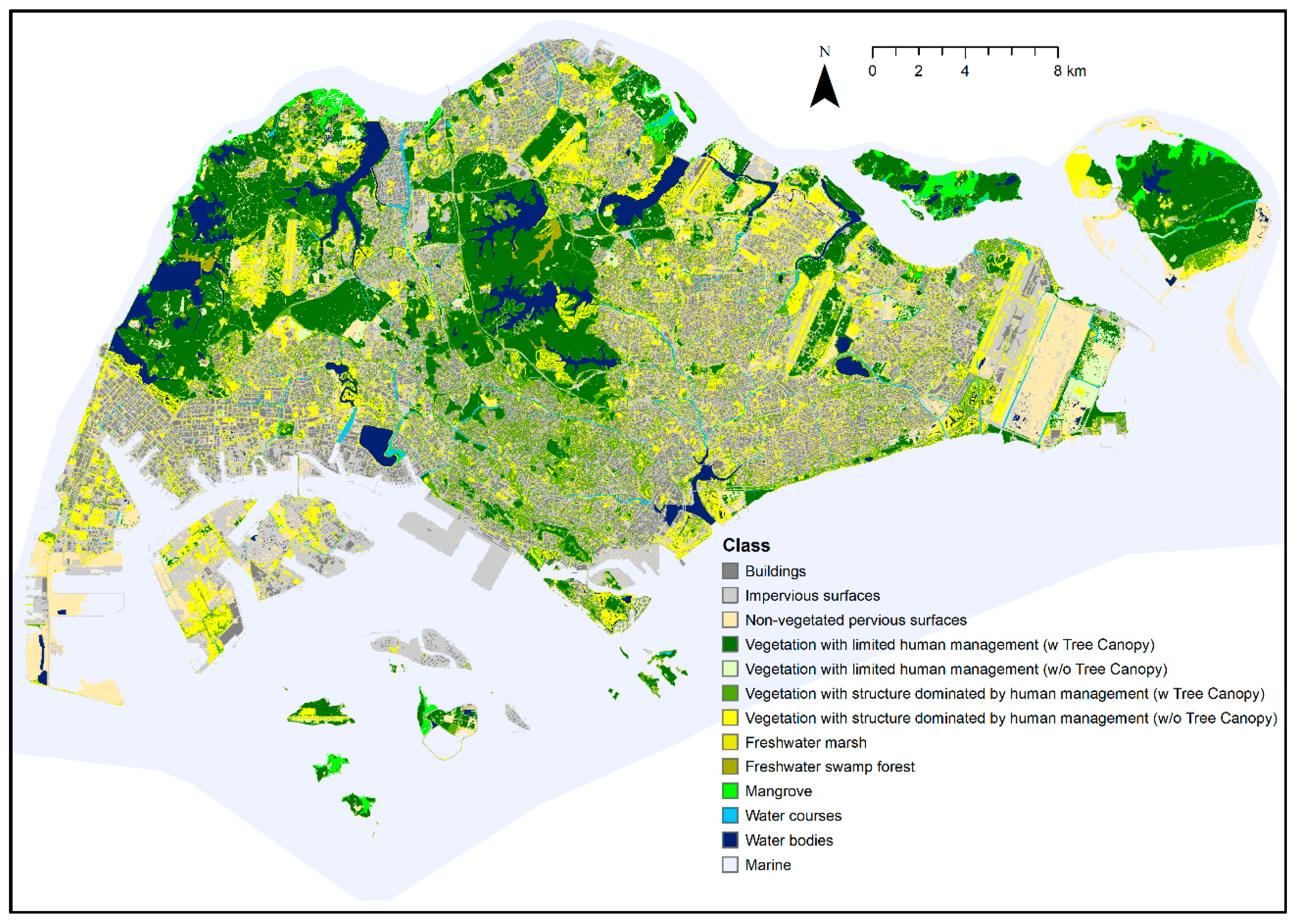
The classified map of high resolution images of Singapore from 2003 to 2018 is shown in Figure 1. The map has a maximum spatial resolution of 30 cm (as per the panchromatic resolution of WorldView-3). The area of each map class is shown in Table 1. The total non-marine area classified was 742.22 km2, of which 359.06 km2 (49 %) was covered by vegetation and 46.63 km2 (6 %) was covered with surface freshwater features. The remaining area was unvegetated land; consisting of built-up impervious surfaces of 284.10 km2 (38 %) and pervious surfaces of 53.00 km2 (7 %).
2.2. Accuracy Assessment
To validate the accuracy of the map produced, random points were generated across the study area to act as validation points. A stratified sample of 80 points per map class was conducted to ensure representativeness of the accuracy assessment. The exceptions to this number were for the freshwater swamp forest and marsh classes where owing to the small area of these ecosystems in Singapore [12], the number of validation points was 40 each instead. Each validation point was visually inspected by an expert using the original satellite imagery, both in true colour and false-coloured infrared. The validation points were compared to the map’s classes using the sample tool and the Cohen’s kappa coefficient statistic and percentage accuracy was calculated to quantify the level of agreement between the map classification and validation sample.
The overall accuracy of the map was 79 % and the kappa coefficient was 77 %. A detailed confusion matrix of the accuracy assessment can be found in Table 2, in which the errors of classification to each map class can be identified. The lowest accuracy classification was that of freshwater marsh; this was most frequently misclassified as water bodies. The highest number of points were misclassified for managed vegetation without tree canopy cover, which was typically misclassified as unmanaged vegetation without tree canopy cover. This is not surprising given the similar taxonomic composition and hence spectral signatures of unmanaged scrub and grass, and managed shrub and turf [13].
The accuracy of the map is comparable with similar studies that classified the land cover of high resolution satellite imagery [14,15]. This study uses 12 land cover classes. When classifying between a larger number of classes, the likelihood of the errors typically increases because the spectral differences between the classes are smaller. Misclassification was most often between classes that are structurally and ecologically very similar, and that cover small areas of Singapore. For example, the class that showed the greatest class error was vegetation with limited human management and no tree canopy (Table 2). This class covers less than 2 % of Singapore’s area, and furthermore was predominately misclassified as vegetation dominated by human management with no tree canopy; a categorization that is functionally very similar in terms of its ecology. The classes with less than 70 % accuracies together occupy less than 10 % of the area (Table 1 and Table 2).
2.3. Data in Perspective
There are many different types of map that can be derived from satellite imagery. This map does not describe land use, but represents ecologically-relevant classes of vegetation and water cover that are intended for use in ecological studies. The classes therefore represent contrasting types of ecosystems that may be expected to have different ecological values. This map is building on the works of references [12,16] that investigate the changing physical landscape of Singapore.
Many users of the map will be interested in broad-scale patterns of vegetation cover in Singapore, so will find their analyses robust to the classification errors reported here. Users interested in particular types of ecosystem should be aware of the uncertainties involved in the classification (Table 2), and may find the dataset unsuitable for studies of some categories (e.g., vegetation with limited human management and without a tree canopy).
3. Methods
This section details the steps in processing satellite imagery of Singapore into a land cover map for natural capital assessment. For the purposes of this study, only the terrestrial, freshwater environments of Singapore will be mapped in detail, while the marine environment that is underwater will be classed as just ‘Marine’. The exception is the mangrove forests, which cross the coastal boundary but generally have at least a part of the vegetation above the water at all times [17]. The classification uses a hybrid approach; first conducting a supervised machine learning to classify broad land cover types, before adding more detailed sub-classes using secondary sources of spatial data.
Singapore is a city-state located in the tropics with its central point at latitude 1.21° N and longitude 103.49° E. The land area of Singapore measures 724.20 km2 [18] that consists of one main island and many smaller islands within its territorial boundary. Singapore’s location near the equator means that satellite images are frequently obstructed by cloud cover due to convection of water vapour in the atmosphere [19]. Hence, it is difficult to find a single cloud-free satellite image of the entire island. Therefore, multiple satellite images acquired over a period of time are needed to provide island-wide coverage. Although the country is highly urbanized, there are many pockets of green spaces in between buildings and tree-lined road networks. Major green spaces in the country are at the Western and Central portions of the main island, and Pulau Ubin and Pulau Tekong in the northeast. As with high-density urban areas around the world, Singapore’s urban form is highly heterogeneous, incorporating industrial commercial and residential land use zones, with a mix of high- and low-rise buildings [20].
3.1. Data Acquisition
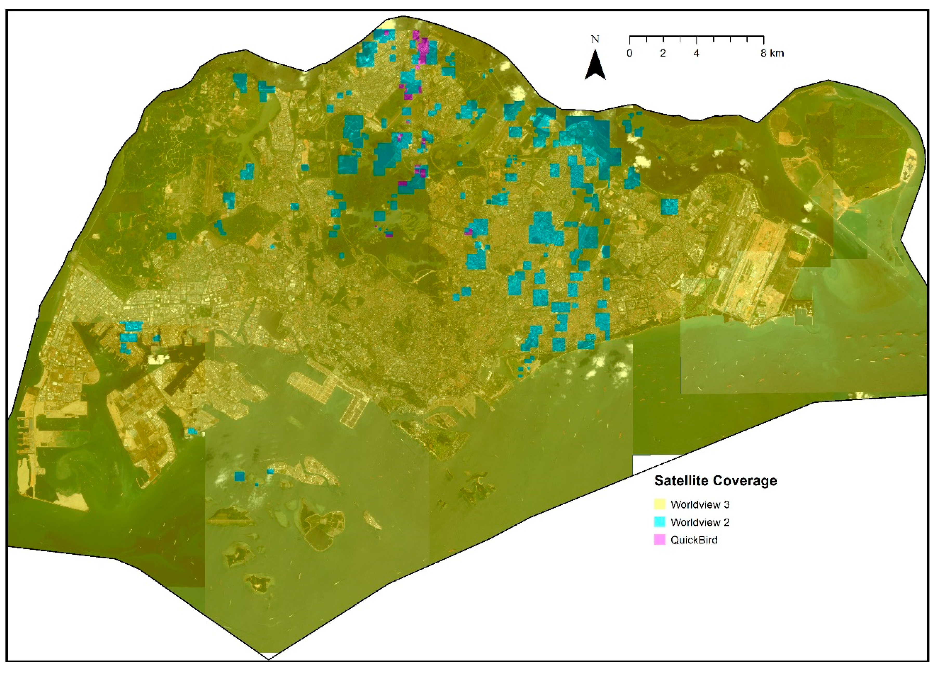
High resolution images of Singapore were downloaded from DigitalGlobe’s ‘Discover’ online search tool (no longer available due to DigitalGlobe’s merger with Maxar). Multiple images were needed (Figure 2 and Table 3) since the swath widths of the WorldView 2 and 3 satellite sensors do not span the entire island. Further, cloud cover obscures parts of all the images. WorldView 2 and 3 capture eight multispectral bands between 400 to 1040 nm (Table 3). The images were taken between 2010 to 2018 by the space-borne WorldView 2 and 3 sensors that have multispectral spatial resolutions of 2.0 and 1.2 m, respectively, and panchromatic spatial resolutions of 0.3 and 0.5 m. Additionally, one image from QuickBird was used to patch an area of cloud cover in the north (Figure 2). The QuickBird image was taken on October 2003; it has a multispectral spatial resolution of 2.5 m and a panchromatic spatial resolution of 0.6 m.
3.2. Image Pre-Processing
The image pre-processing described in this section was done in ArcGIS Desktop 10.5 [21]. To prepare the images for classification, areas obscured by clouds were removed by visual inspection. Polygons were drawn around cloudy areas and their shadows as the reflectance in the latter areas are affected by cloud-obscurity. The polygons were then clipped from the image and reflectance corrected with the apparent reflectance function from the image analysis tool [22]. There was a total of 17 different images taken from different dates to classify.
3.3. Image Classification
A summary of the object based image classification detailed in this section is presented in Figure 3. To classify high resolution imagery, an object-based approach was used instead of a pixel-based classification technique, to avoid ‘salt and pepper’ effects on the resultant map [23]. To segment images into objects, a means-shift approach was applied using the segment means-shift function [24] in ArcGIS. In the parameters of the function, spectral and spatial details were both given maximum importance (set as 20.0 and 1.0, respectively) to discriminate as best as the function can between features in the landscape, for example, trees and grass [25]. The spectral detail setting was used in means-shift segmentation to discriminate objects based on spectral signatures [25]. The spatial detail setting was used to discriminate objects based on the shape of the features to produce sharper segments, like buildings and roads within impervious surfaces [25]. A minimum mapping unit of 300 pixels (approximately 5 m2) was set to save on processing time and storage space. Since the function can only read three bands in a composite raster to be segmented, the multispectral bands of near infrared (760–900 nm), red (630–690 nm), and green (510–600 nm) were used to focus on discriminating vegetation features. The segmentation produced 25,882,810 objects in the study area that were visually checked to ensure that they enveloped a meaningful object (e.g., building outlines, jetties, and grass patches).
Next, the data from the multispectral satellite image bands were added as attributes to each object to be classified. The zonal statistics function was used to calculate the median of each of the multispectral band pixel values from all pixels within the objects created. Eight multispectral bands were available for the WorldView images [26], while four were available for the QuickBird images [27]. The objects were exported to R statistical software 3.5.3 [28].
Five broad-level land and water cover types were initially classified using a supervised method using a random forest algorithm 4.6 [29]. The classes were impervious surfaces; pervious bare surfaces; trees; grass; water. Shadows cast by tall buildings and trees were also classified as a separate class. A separate random forest classification was conducted for each image individually. To train the random forest classifier, at least 150 objects were visually selected for each class by hand on ArcGIS Desktop. Hence each image would have at least 900 training points. The random forests were built with 500 trees with two variables tried at each split [29]. The out-of-box (OOB) estimates of error rate were all less than 10% for each image classified. The 17 classified images were then mosaicked together starting with the earliest image (Image 901) in ascending date order (Table 3) with the most recent imagery replacing areas of overlap.
The precision of land cover was further refined into land use classes with data inputs from other sources. Shadows were first dealt with using the zonal statistics to estimate which of the five preceding land cover classes lie in it. The remaining patches of shadows that were not fixed were re-classified manually based on cross referencing to Google Earth Images (that are also high resolution) and local knowledge of the area. Impervious surfaces were refined into buildings with building footprint information downloaded from OpenStreetMap [30]. Areas of vegetation were also divided between managed and unmanaged vegetation by manually digitizing 2014 SPOT5 satellite image of Singapore based on ground-truthing and a previous lower-resolution vegetation map of Singapore [12]. Vegetated areas that intersected with swamp and marsh classes from the aforementioned map of Singapore [12] were reclassified as these classes accordingly. Inland freshwater ecosystems were manually reclassified into water courses (rivers, canals, drains) and water bodies (lakes, reservoirs, swimming pools) based on knowledge of the freshwater network [31].
Finally, the map was error-checked and manually corrected with on screen digitization and rectification of errors in classification. This was done systematically with a regular grid laid out across the study area with a size of 1990 m by 1200 m. The map classification within every one of the 649 grids was manually checked for classification errors at a map scale of 1:5500. The erroneous raster pixels were edited using the raster painting [32] tool in ArcGIS to selectively convert misclassified raster pixels to the correct ones.
4. User Notes
The image segmentation applied a minimum mapping unit of 300 pixels, approximately 5 m2. This translates approximately to the size of a tree canopy. Nonetheless, no restraints were imposed on the configurations to the 300 pixels that made an object and thus, 300 pixels were not always square in configuration but may represent a row of shrubs or hedges. This minimum mapping unit threshold may cause vegetated sections smaller than 300 pixels (such as small trees or shrubs) to be neglected. While urban vegetation patches are small and heterogeneous, most vegetated areas are nonetheless larger than 5 m2 and are thus discernible using this approach. Furthermore, it would be too computationally intensive to decrease the minimum mapping unit; the current analysis took two weeks to conduct the segmentation using a high-spec desktop PC (four cores and 16 GB of RAM), further computational time would be required to add data values to each segment.
With mapping of the earth’s surface at such high spatial resolution, errors of accuracy and precision are bound to occur. For maps derived from remote sensing, accuracy assessments are integral to data reporting [33]. This study has adopted Congalton’s and Green’s [34] rules of thumb for such accuracy assessments where at least 30 validation points were sampled per map class. Their works focused largely on global land cover maps where accuracy depends on many factors including number of classes, quality of remotely sensed data and validation techniques, and classification methods [34]. In a city-scale study by Myint and colleagues [35], 100 points per class (similar to 80 points per class in this study) were used to evaluate the accuracy of different classification methods. The accuracy assessed in this study is comparable to other studies using high resolution imagery (75 % to 86 % [36]), and similar to a previous map of Singapore’s vegetation types [12]. The accuracy reported in the previous Singapore mapping study was slightly higher; 86 % to 90 % with a Kappa coefficient of 79 % to 86 %, but this is likely due to the lower number of classes used (five compared to 13 in this study) [12].
The satellite composite used to build the map was captured over a period of eight years, except Image 901 that was captured 15 years before the latest image. In rapidly-changing areas like cities, this can cause mismatches between the classification in overlapping areas, and cause artefacts where two images are composited across an area that changed between the two dates; such as areas that were under construction (pervious unvegetated) and were later built (impervious vegetated). Furthermore, because Singapore is located near the equator where cloud cover constantly obscures satellite imagery, images taken at different dates and times are necessary to build a cloud free map of the entire country [19].
A further issue in an urban setting is caused by tall buildings obscuring shorter objects below. Images from satellite imagery are rarely taken at nadir and tall buildings blocks the view of objects at ground level such as trees, shrubs, and roads [37]. Such building “shadows” also conceal objects below. This is an issue in high-rise parts of Singapore, especially in the central business district where the tallest buildings are in close proximity. Orthorectification was not possible in this study due to the lack of overlapping imagery that was also free of clouds.
Author Contributions
Conceptualization, D.R. and L.G.; methodology, D.R. and L.G.; validation, L.G. and A.Y.; formal analysis, D.R. and L.G.; resources, D.R. and A.Y.; data curation, L.G. and A.Y.; writing—original draft preparation, L.G. and D.R.; writing—review and editing, D.R., L.G. and A.Y.; visualization, L.G.; supervision, D.R.; project administration, D.R.; funding acquisition, D.R.
Funding
This research is supported by the National Research Foundation, Prime Minister’s Office, Singapore under its Campus for Research Excellence and Technological Enterprise (CREATE) Programme (NRF2016-ITC001-013).
Acknowledgments
High resolution satellite imagery was provided courtesy of the DigitalGlobe Foundation (www.digitalglobefoundation.org). A.Y. would like to thank Ting Ying Ying and Gabriel Lim for their assistance in digitising the managed vegetation areas.
Conflicts of Interest
The authors declare no conflict of interest.
References
- Seto, K.C.; Fragkias, M.; Güneralp, B.; Reilly, M.K. A Meta-Analysis of Global Urban Land Expansion. PLoS ONE 2011, 6, e23777. [Google Scholar] [CrossRef]
- Grimm, N.B.; Faeth, S.H.; Golubiewski, N.E.; Redman, C.L.; Wu, J.; Bai, X.; Briggs, J.M. Global Change and the Ecology of Cities. Science 2008, 319, 756–760. [Google Scholar] [CrossRef] [Green Version]
- Song, X.P.; Tan, P.Y.; Edwards, P.; Richards, D. The economic benefits and costs of trees in urban forest stewardship: A systematic review. Urban For. Urban Green. 2018, 29, 162–170. [Google Scholar] [CrossRef]
- Hoellein, T.; Rojas, M.; Pink, A.; Gasior, J.; Kelly, J. Anthropogenic Litter in Urban Freshwater Ecosystems: Distribution and Microbial Interactions. PLoS ONE 2014, 9, e98485. [Google Scholar] [CrossRef]
- Freeman, C. Geographic information systems and the conservation of urban biodiversity. Urban Policy Res. 1999, 17, 51–60. [Google Scholar] [CrossRef]
- Bolund, P.; Hunhammar, S. Ecosystem services in urban areas. Ecol. Econ. 1999, 29, 293–301. [Google Scholar] [CrossRef]
- Jenerette, G.D.; Harlan, S.L.; Stefanov, W.L.; Martin, C.A. Ecosystem services and urban heat riskscape moderation: Water, green spaces, and social inequality in Phoenix, USA. Ecol. Appl. 2011, 21, 2637–2651. [Google Scholar] [CrossRef]
- Keesstra, S.; Nunes, J.; Novara, A.; Finger, D.; Avelar, D.; Kalantari, Z.; Cerdà, A. The superior effect of nature based solutions in land management for enhancing ecosystem services. Sci. Total Environ. 2018, 610–611, 997–1009. [Google Scholar] [CrossRef]
- Thiagarajah, J.; Wong, S.K.M.; Richards, D.R.; Friess, D.A. Historical and contemporary cultural ecosystem service values in the rapidly urbanizing city state of Singapore. Ambio 2015, 44, 666–677. [Google Scholar] [CrossRef] [Green Version]
- Li, D.; Ke, Y.; Gong, H.; Li, X. Object-Based Urban Tree Species Classification Using Bi-Temporal WorldView-2 and WorldView-3 Images. Remote Sens. 2015, 7, 16917–16937. [Google Scholar] [CrossRef] [Green Version]
- Busetto, L.; Meroni, M.; Colombo, R. Combining medium and coarse spatial resolution satellite data to improve the estimation of sub-pixel NDVI time series. Remote Sens. Environ. 2008, 112, 118–131. [Google Scholar] [CrossRef]
- Yee, A.T.K.; Corlett, R.T.; Liew, S.C.; Tan, H.T.W. The vegetation of Singapore―An updated map. Gard. Bull. Singap. 2011, 63, 205–212. [Google Scholar]
- Fuller, R.M.; Groom, G.B.; Jones, A.R. The land-cover map of great Britain: An automated classification of landsat thematic mapper data. Photogramm. Eng. Remote. Sens. 1994, 60, 553–562. [Google Scholar]
- Liu, X.; He, J.; Yao, Y.; Zhang, J.; Liang, H.; Wang, H.; Hong, Y. Classifying urban land use by integrating remote sensing and social media data. Int. J. Geogr. Inf. Sci. 2017, 31, 1675–1696. [Google Scholar] [CrossRef]
- Randall, M.; Fensholt, R.; Zhang, Y.; Bergen Jensen, M. Geographic Object Based Image Analysis of WorldView-3 Imagery for Urban Hydrologic Modelling at the Catchment Scale. Water 2019, 11, 1133. [Google Scholar] [CrossRef]
- Yee, A.T.K.; Chong, K.Y.; Neo, L.; Tan, H.T.W. Updating the classification system for the secondary forests of Singapore. Raffles Bull. Zool. 2016, 32, 11–21. [Google Scholar]
- Lovelock, C.E.; Cahoon, D.R.; Friess, D.A.; Guntenspergen, G.R.; Krauss, K.W.; Reef, R.; Rogers, K.; Saunders, M.L.; Sidik, F.; Swales, A.; et al. The vulnerability of Indo-Pacific mangrove forests to sea-level rise. Nature 2015, 526, 559–563. [Google Scholar] [CrossRef] [Green Version]
- Singapore Land Authority (SLA). Total Land Area of Singapore. Available online: https://data.gov.sg/dataset/total-land-area-of-singapore (accessed on 24 April 2019).
- Asner, G.P. Cloud cover in Landsat observations of the Brazilian Amazon. Int. J. Remote Sens. 2001, 22, 3855–3862. [Google Scholar] [CrossRef]
- Tan, P.Y.; Wang, J.; Sia, A. Perspectives on five decades of the urban greening of Singapore. Cities 2013, 32, 24–32. [Google Scholar] [CrossRef]
- Environmental Systems Research Institute (ESRI). ArcGIS Release 10.5; Environmental Systems Research Institute (ESRI): Redlands, CA, USA, 2016. [Google Scholar]
- Environmental Systems Research Institute (ESRI). Apparent Reflectance Function. Available online: http://desktop.arcgis.com/en/arcmap/10.5/manage-data/raster-and-images/apparent-reflectance-function.htm (accessed on 2 May 2019).
- Liu, D.; Xia, F. Assessing object-based classification: Advantages and limitations. Remote Sens. Lett. 2010, 1, 187–194. [Google Scholar] [CrossRef]
- Environmental Systems Research Institute (ESRI). Segment Mean Shift Function. Available online: http://desktop.arcgis.com/en/arcmap/10.5/manage-data/raster-and-images/segment-mean-shift-function.htm (accessed on 24 April 2019).
- Butler, K. Pass the Classification but Hold the Salt and Pepper. Available online: https://www.esri.com/arcgis-blog/products/product/national-government/pass-the-classification-but-hold-the-salt-and-pepper/ (accessed on 17 July 2019).
- DigitalGlobe. WorldView-3 Data Sheet. Available online: http://satimagingcorp.s3.amazonaws.com/site/pdf/WorldView3-DS-WV3-Web.pdf (accessed on 17 July 2019).
- Satellite Imaging Corporation. QuickBird Imagery Products FAQ. Available online: http://satimagingcorp.s3.amazonaws.com/site/pdf/quickbird_imagery_products.pdf (accessed on 17 July 2019).
- R Core Team. R: A Language and Environment for Statistical Computing; R Foundation for Statistical Computing: Vienna, Austria, 2014. [Google Scholar]
- Liaw, A.; Wiener, M. Classification and regression by randomForest. R News 2002, 2, 18–22. [Google Scholar]
- OpenStreetMap. OpenStreetMap of Singapore. Available online: https://www.openstreetmap.org/search?query=singapore#map=12/ 1.2905/103.8520 (accessed on 5 April 2018).
- Public Utilities Board (PUB). Drainage Network. Available online: https://www.pub.gov.sg/drainage/network (accessed on 24 April 2019).
- Environmental Systems Research Institute (ESRI). About Using the Raster Painting Tools. Available online: http://desktop.arcgis.com/en/arcmap/10.5/extensions/arcscan/using-the-raster-painting-tools-about-using-the-ra.htm (accessed on 24 April 2019).
- Congalton, R.G. A review of assessing the accuracy of classifications of remotely sensed data. Remote Sens. Environ. 1991, 37, 35–46. [Google Scholar] [CrossRef]
- Congalton, R.G.; Green, K. Sample Design Considerations. In Assessing the Accuracy of Remotely Sensed Data: Principles and Practices, 2nd ed.; CRC Press: New York, NY, USA, 2009; pp. 63–103. [Google Scholar]
- Myint, S.W.; Gober, P.; Brazel, A.; Grossman-Clarke, S.; Weng, Q. Per-pixel vs. object-based classification of urban land cover extraction using high spatial resolution imagery. Remote Sens. Environ. 2011, 115, 1145–1161. [Google Scholar] [CrossRef]
- Ma, L.; Li, M.; Ma, X.; Cheng, L.; Du, P.; Liu, Y. A review of supervised object-based land-cover image classification. ISPRS J. Photogramm. Remote Sens. 2017, 130, 277–293. [Google Scholar] [CrossRef]
- Zhang, W.; Li, W.; Zhang, C.; Hanink, D.M.; Li, X.; Wang, W. Parcel-based urban land use classification in megacity using airborne LiDAR, high resolution orthoimagery, and Google Street View. Comput. Environ. Urban Syst. 2017, 64, 215–228. [Google Scholar] [CrossRef] [Green Version]
Figure 1.
The classified map of Singapore made from satellite images taken from 2003 to 2018.

Figure 2.
The geographical coverage of high resolution satellite images used for this study.

Figure 3.
A flowchart of classifying high resolution satellite imagery into the land cover map. The image sample was taken from a WorldView 3 image (ID 301).
Figure 3.
A flowchart of classifying high resolution satellite imagery into the land cover map. The image sample was taken from a WorldView 3 image (ID 301).


Table 1.
A list of map classes with their surface areas.
| Map Class | Code | Area (km2) | Percentage of Land Area (%) |
|---|---|---|---|
| Buildings | 1 | 91.1 | 12.3 |
| Artificial impervious surfaces | 2 | 193.0 | 26.0 |
| Non-vegetated pervious surfaces | 3 | 53.0 | 7.1 |
| Vegetation with limited human management (with Tree Canopy) | 4 | 139.0 | 18.7 |
| Vegetation with limited human management (without Tree Canopy) | 5 | 14.1 | 1.9 |
| Vegetation with structure dominated by human management (with Tree Canopy) | 6 | 82.8 | 11.1 |
| Vegetation with structure dominated by human management (without Tree Canopy) | 7 | 112.5 | 15.1 |
| Freshwater swamp forest | 8 | 2.2 | 0.3 |
| Freshwater marsh | 9 | 0.4 | 0.1 |
| Mangrove forest | 10 | 8.1 | 1.1 |
| Water courses | 11 | 8.2 | 1.1 |
| Water bodies | 12 | 38.4 | 5.2 |
| Marine | 13 | 647.4 | - |
Table 2.
The confusion matrix for this map’s accuracy assessment. The acronyms used in this table are: UA for user accuracy; PA for producer accuracy; CE for commission errors; and OE for omission errors.
Table 2.
The confusion matrix for this map’s accuracy assessment. The acronyms used in this table are: UA for user accuracy; PA for producer accuracy; CE for commission errors; and OE for omission errors.
| 1 | 2 | 3 | 4 | 5 | 6 | 7 | 8 | 9 | 10 | 11 | 12 | Total | UA | CE | |
|---|---|---|---|---|---|---|---|---|---|---|---|---|---|---|---|
| 1 | 71 | 4 | 2 | 77 | 92% | 8% | |||||||||
| 2 | 8 | 68 | 16 | 3 | 1 | 8 | 104 | 65% | 35% | ||||||
| 3 | 7 | 53 | 4 | 1 | 65 | 82% | 18% | ||||||||
| 4 | 3 | 78 | 3 | 5 | 1 | 1 | 1 | 92 | 85% | 15% | |||||
| 5 | 1 | 18 | 19 | 95% | 5% | ||||||||||
| 6 | 1 | 3 | 6 | 65 | 1 | 1 | 77 | 84% | 16% | ||||||
| 7 | 1 | 2 | 46 | 8 | 80 | 137 | 58% | 42% | |||||||
| 8 | 1 | 36 | 6 | 43 | 84% | 16% | |||||||||
| 9 | 7 | 7 | 100% | 0% | |||||||||||
| 10 | 63 | 2 | 65 | 97% | 3% | ||||||||||
| 11 | 3 | 26 | 9 | 77 | 2 | 117 | 66% | 34% | |||||||
| 12 | 1 | 76 | 77 | 99% | 1% | ||||||||||
| Total | 80 | 80 | 80 | 80 | 80 | 80 | 80 | 40 | 40 | 80 | 80 | 80 | 880 | ||
| PA | 89% | 85% | 66% | 98% | 23% | 81% | 100% | 90% | 18% | 79% | 96% | 95% | Overall | 79% | |
| OE | 11% | 15% | 34% | 3% | 78% | 19% | 0% | 10% | 83% | 21% | 4% | 5% | Kappa | 77% |
Table 3.
Information of the satellite imagery classified in this study sorted by acquisition date.
| Sensor | Image ID | Date | Time (GMT+8) | Wavelength (nm) | Coverage (%) |
|---|---|---|---|---|---|
| WorldView-3 | 308 | 18 Feb 18 | 1138 h | 400–1040 | 0.17 |
| WorldView-3 | 302 | 10 Feb 18 | 1158 h | 400–1040 | 31.07 |
| WorldView-3 | 305 | 10 Feb 18 | 1157 h | 400–1040 | 19.99 |
| WorldView-3 | 307 | 10 Feb 18 | 1158 h | 400–1040 | 7.38 |
| WorldView-3 | 306 | 15 Nov 17 | 1106 h | 400–1040 | 9.56 |
| WorldView-3 | 301 | 5 May 17 | 1152 h | 400–1040 | 11.97 |
| WorldView-3 | 304 | 12 Nov 16 | 1145 h | 400–1040 | 1.88 |
| WorldView-3 | 303 | 29 Jun 16 | 1141 h | 400–1040 | 1.18 |
| WorldView-2 | 208 | 19 Apr 15 | 1136 h | 400–1040 | 1.00 |
| WorldView-2 | 203 | 23 Mar 15 | 1134 h | 400–1040 | 0.01 |
| WorldView-2 | 207 | 23 Mar 15 | 1133 h | 400–1040 | 0.67 |
| WorldView-2 | 206 | 17 Jan 15 | 1133 h | 400–1040 | 1.97 |
| WorldView-2 | 201 | 14 Jun 12 | 1143 h | 400–1040 | 0.27 |
| WorldView-2 | 202 | 18 Jul 11 | 1149 h | 400–1040 | 0.26 |
| WorldView-2 | 204 | 8 Apr 11 | 1143 h | 400–1040 | 0.11 |
| WorldView-2 | 205 | 19 Nov 10 | 1138 h | 400–1040 | 0.11 |
| QuickBird | 901 | 16 Oct 03 | 1115 h | 450–900 | 0.17 |
© 2019 by the authors. Licensee MDPI, Basel, Switzerland. This article is an open access article distributed under the terms and conditions of the Creative Commons Attribution (CC BY) license (http://creativecommons.org/licenses/by/4.0/).
Share and Cite
MDPI and ACS Style
Gaw, L.Y.-F.; Yee, A.T.K.; Richards, D.R. A High-Resolution Map of Singapore’s Terrestrial Ecosystems. Data 2019, 4, 116. https://0-doi-org.brum.beds.ac.uk/10.3390/data4030116
AMA Style
Gaw LY-F, Yee ATK, Richards DR. A High-Resolution Map of Singapore’s Terrestrial Ecosystems. Data. 2019; 4(3):116. https://0-doi-org.brum.beds.ac.uk/10.3390/data4030116
Chicago/Turabian StyleGaw, Leon Yan-Feng, Alex Thiam Koon Yee, and Daniel Rex Richards. 2019. "A High-Resolution Map of Singapore’s Terrestrial Ecosystems" Data 4, no. 3: 116. https://0-doi-org.brum.beds.ac.uk/10.3390/data4030116