Predicting High-Risk Prostate Cancer Using Machine Learning Methods

Abstract

Prostate cancer can be low- or high-risk to the patient’s health. Current screening on the basis of prostate-specific antigen (PSA) levels has a tendency towards both false positives and false negatives, both of which have negative consequences. We obtained a dataset of 35,875 patients from the screening arm of the National Cancer Institute’s Prostate, Lung, Colorectal, and Ovarian Cancer Screening Trial. We segmented the data into instances without prostate cancer, instances with low-risk prostate cancer, and instances with high-risk prostate cancer. We developed a pipeline to deal with imbalanced data and proposed algorithms to perform preprocessing on such datasets. We evaluated the accuracy of various machine learning algorithms in predicting high-risk prostate cancer. An accuracy of 91.5% can be achieved by the proposed pipeline, using standard scaling, SVMSMOTE sampling method, and AdaBoost for machine learning. We then evaluated the contribution of rate of change of PSA, age, BMI, and filtration by race to this model’s accuracy. We identified that including the rate of change of PSA and age in our model increased the area under the curve (AUC) of the model by 6.8%, whereas BMI and race had a minimal effect.

1. Introduction

Prebiopsy screening of prostate cancer is used because biopsies, which confirm whether there is cancer present, are potentially harmful to patients who do not have prostate cancer since they may cause infections in people who have them [1,2,3]. One very common screening method is the measurement of prostate-specific antigen (PSA), which is a protein produced by cells of the prostate gland. However, it has been shown that monitoring PSA levels has no significant impact on prostate cancer mortality after a median follow-up of 10 years with those who had this monitoring [4,5]. The United States Preventative Services Task Force (USPSTF) originally issued a recommendation against PSA screening for all ages in 2012 [6], but in 2017 revised that recommendation to say that the decision to undergo PSA testing is an individual decision for men between 55 and 69 years of age, with those over 70 still being recommended against PSA screening [1]. “Cancer Screening: Theory and Applications” by Auvinen and Hakama presents a skeptical view of the efficacy of PSA screening, claiming that it doesn’t save many years of life in the long run [7]. Negoita et al. find that decrease in PSA screening following the aforementioned USPSTF recommendations has led to a flattening off of mortality, although this could be due to other factors, and has also led to a higher incidence of late stage disease [8]. Martin et al. see promise in developing “better screening tests (including free (unbound) PSA and biochemical and genetic markers), clear protocols for active surveillance, better focal treatments for localized diseases, and better treatments for advanced cancer” [5]. The defects in PSA screening thus warrant investigation into new screening methods.

One screening method is magnetic resonance imaging (MRI), which has the potential to identify that someone with raised PSA levels actually has a low-risk cancer and hence does not need to have a biopsy [9,10,11]. Rundo et al. have recently suggested automating the prostate segmentation component of MRI by using a technique based on the fuzzy c-means clustering algorithm, which would improve the time efficiency of MRI screening [11]. Several methods have also been suggested to improve PSA testing, such as age-specific PSA testing, factoring in the ratio of free PSA (that is, PSA not bound to other proteins) to total PSA (the total level of PSA, including both free and bound PSA), and factoring the rate of change of PSA into screening, although the NCI reports that neither of these methods have been conclusively proven to decrease the risk of death [3].

We aim to test the efficacy of machine learning methods for prostate cancer screening using various clinical measurements. We also aim to determine the effect that variables such as BMI, race, rate of change, and age have on the model’s accuracy.

2. Literature Review

In 2017, Shoaibi et al. used a PSA growth curve to predict high-risk prostate cancer, training their model on the National Cancer Institute PLCO dataset, and using a dataset of 680,390 veterans as the validation set [12]. They performed a statistical analysis on a non-linear mixed regression model built with age, race, baseline PSA, and BMI as adjustment factors. In 2018, Roffman et al. developed an artificial neural network (ANN) to predict the risk of prostate cancer on the basis of “age, BMI, diabetes status, smoking status, emphysema, asthma, race, ethnicity, hypertension, heart disease, exercise habits, and history of stroke,” using the National Health Interview Survey (NHIS) adult survey data as training and validation set [13]. In the same year, PSA was used by Wang et al. together with age, result of digital rectal examination and transrectal ultrasound, and prostate volume to predict both significant, benign, and insignificant cancer (both significant vs. benign and insignificant and significant vs. benign vs. insignificant) on a dataset of 1652 Chinese men with biopsies [2]. These variables were used in four algorithms (support vector machine, random forests, least squares support vector machine, and artificial neural network). All algorithms achieved >0.93 accuracy for the prediction of significant versus benign and insignificant, and >0.79 for prediction of benign versus insignificant versus significant prostate cancer.

Many other attempts to predict the outcomes related to prostate cancer diagnosis from clinical data using machine learning methods are trained on severely imbalanced datasets because of the rarity of prostate cancer, and do not use the rate of change of PSA as a feature [14,15]. We aim to apply machine learning methods to predict the presence of prostate cancer based on variables available in clinical data which may be attained without biopsies. Our work differentiates itself from other studies in the following respects. First, we are applying a wide range of machine learning prediction methods to a model featuring rate of change of PSA, which Shoaibi et al. did not do. Conversely, we are applying the rate of change of PSA variable in prediction using machine learning methods, which other machine learning methods for prostate cancer screening have not done. Moreover, we apply imbalance correction methods to the dataset and evaluate these methods based on their impact on the sensitivity and specificity of the classifiers.

3. Data Description

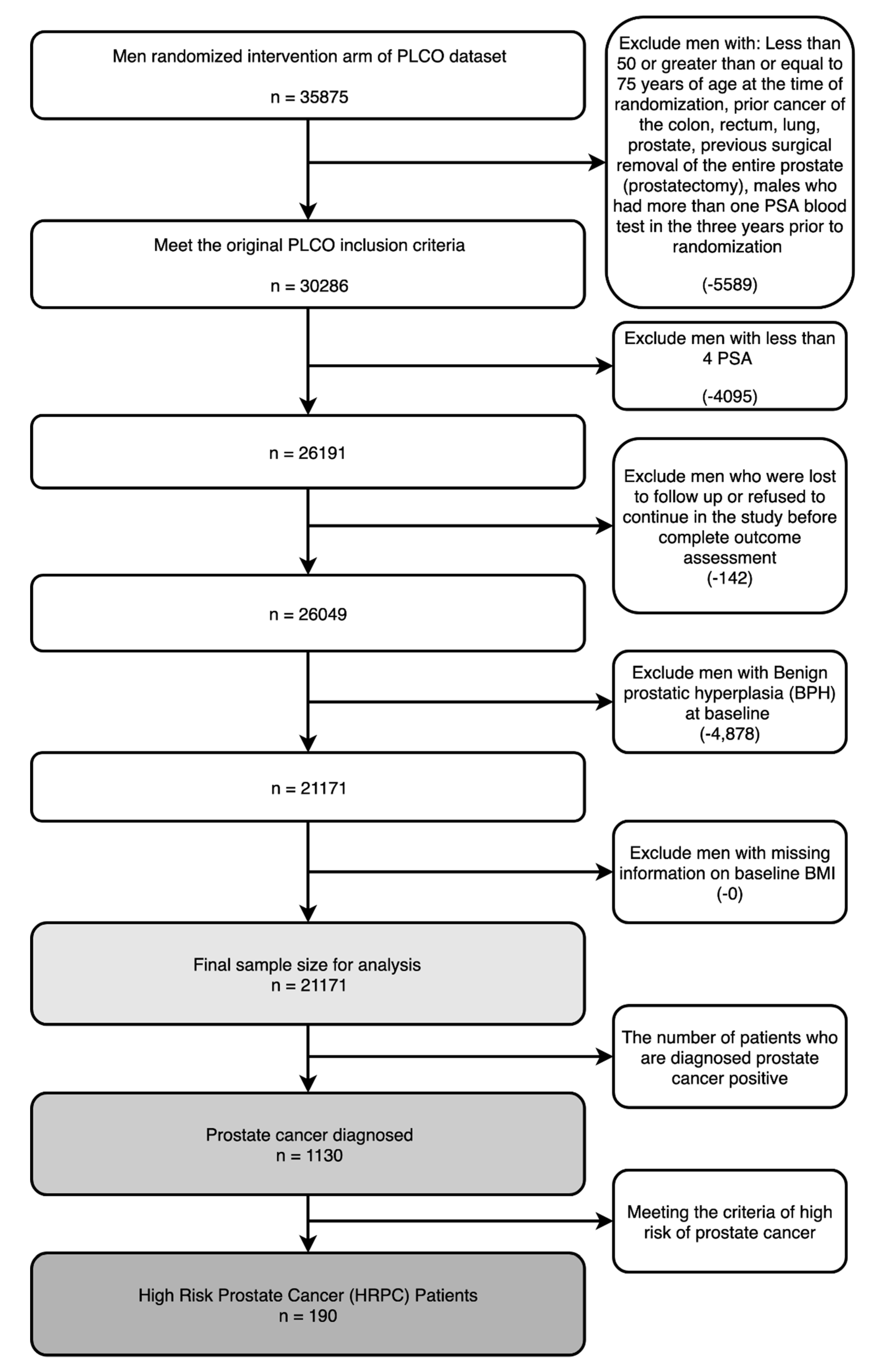
In this study, we built machine learning models on the screening arm of the prostate component of The National Cancer Institute’s (NCI’s) Prostate, Lung, Colorectal, and Ovarian Cancer Screening Trial (PLCO). We used the same inclusion and exclusion criteria as Shoaibi et al. The criteria used are presented in Figure 1. The number of patients in the dataset, upon the different inclusion/exclusion criteria, are displayed under the criteria in each box. It should be noted that the numbers they reported having in the dataset did not align with ours, with them starting with 38,340 entries in the intervention arm and, after applying the inclusion and exclusion criteria, having 20,888 entries in the dataset. Furthermore, we could not find out how to determine whether patients had “suspicious screening results that do not have correspondent complete diagnostic procedures and final results” [12].

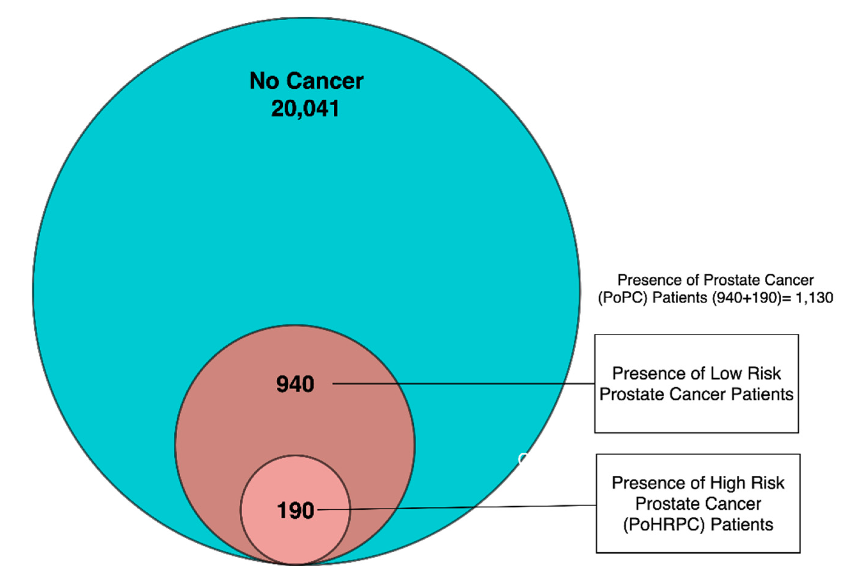
We have split this dataset into three groups: instances without prostate cancer, instances with low-risk prostate cancer, and instances with high-risk prostate cancer. High-risk cancers are cancers where the cancer cells spread at a fast rate, leading to a high possibility of mortality and therefore calling for immediate treatment as opposed to the active surveillance that is often thought to be suitable for low-risk cancer [16]. The definition of high-risk prostate cancer that we used, following Shoaibi et al. was Gleason score > 7, PSA level ≥ 20 ng/mL, cancer invading the prostate capsule, or involving more than one lobe [12]. It should be noted that only the first two of these criteria were reported in the dataset. The segmentation of the data is represented in Figure 2.

We developed two machine learning models (i) testing the presence of cancer and (ii) testing presence of high-risk cancer. For the two machine learning models we labelled the dataset in two ways. In the first model, instances without prostate cancer were labelled negative and those with low-risk or high-risk prostate cancer were labelled positive, and this labelled dataset was called presence of prostate cancer (PoPC). In the second model, only instances with high-risk cancer were labelled positive, and those without prostate cancer or with low-risk prostate cancer were labelled negative, and this labelled dataset was called presence of high-risk prostate cancer (PoHRPC). As presented in Figure 1, the dataset had 1130 entries diagnosed with PoPC, out of which only 190 met the criteria of PoHRPC, meaning 0.89% of our dataset in PoHRPC was labelled positive, while 5.34% of our dataset in PoPC was labelled positive.

4. Method

After the initial preprocessing involving handling of misisng values and calculating the rate of change, we determined optimal data imbalance methods and scaling methods by evaluating their effectiveness on the PoPC-labelled dataset. These methods were then implemented on PoHRPC-labelled data. The process of performing our analysis is described in detail here and is presented visually in Figure 3.

4.1. Data Preprocessing

One component of preprocessing was the calculation of Overall ROC and Recent ROC for the patients in the dataset, along with the handling of missing values. The other step in preprocessing was running imbalance correction and scaling methods.

4.1.1. Handling Missing Values

Rather than discard rows with missing values, we used the sklearn Iterative Imputer class with a decision tree regressor to transform the missing value for that row into some value computed by non-linear regression for that row [17]. For datasets that are imbalanced like the ones we are using, this method is better than Simple Imputer, which assigns missing values by using the mean values of columns.

4.1.2. Calculation of Rate of Change

There were six PSA measurements in the PLCO dataset (labelled P₁-P₆). In addition, we calculated two rate of change features, the overall rate of change (Overall ROC) and the recent rate of change (Recent ROC). Overall ROC was calculated by dividing the increase in total PSA level from the oldest reading (P₁) to the latest (P₆) by the number of days that had elapsed between them:

$$Overall ROC=\frac{P_6-P_1}{\#Days}$$

(1)

Second, Recent rate of change (Recent ROC) was the increase in PSA level from the second most recent PSA reading (P₅) to the latest (P₆) divided by the number of days that had elapsed between them:

$$Recent ROC=\frac{P_6-P_5}{\#Days}$$

(2)

4.1.3. Data Imbalance Methods

As shown in Figure 1, the number of negative instances in the dataset is much larger than the number of positive instances. Classifiers built on such imbalanced data might be biased towards negative prediction and therefore have a high proportion of false negative predictions and are unable to generalize to new data. In order to solve this problem, a range of methods for handling data imbalance should be used. The main methods for sampling-based imbalance correction can be broken into the categories of oversampling (where the smaller class has more data added to it to make it the same size as the larger class, often by the data being created) and undersampling (where the larger dataset is sampled from to build a representative set that is the same size as the smaller class) [18]. We used a wide range of oversampling, under-sampling, and combination (featuring elements of both) methods to evaluate which would be the best. All methods were implemented by imbalanced-learn [19]. The full list of methods tested is:

No method, Cluster Centroids (CC), Random Under Sampler (RUS), Near Miss 1 (NM1), Near Miss 2 (NM2), Near Miss3 (NM3), Instance Hardness Threshold (IHT), Repeated Edited Nearest Neighbors (RENN), Random Over Sampler (ROS), SMOTE [20], Borderline SMOTE 1 (BS1) [21], Borderline SMOTE 2 (BS2), ADASYN, SMOTEENN [22], SVMSMOTE [23], SMOTENC, and SMOTETomek.

For each method, we first generated a range of distributions according to the scaling methods listed in Section 4.1.4. We then determined the optimal scaling method for a given sampling method by splitting the data into training and test sets with test size 0.25, running the sampling algorithm in question on the training set, running every classifier in our suite on it, and reported the average area under the curve (AUC) and average accuracy (avg_auc and avg_acc) attained across all classifiers. Whichever scaling method produced the highest average of avg_auc and avg_acc was deemed the optimal method (opt_scaling) for this sampling method, and to evaluate the sampling methods we reported the opt_scaling (avg_auc) and opt_scaling (avg_acc) for it. These metrics were reported in a table, and we also plotted, for each sampling algorithm, the avg_auc against the avg_acc attained across classifiers on data scaled by the optimal scaling method for that sampling algorithm, and then sampled by that sampling algorithm before training. We decided on which sampling method to use from this plot.

When using oversampling and undersampling in cross-validation later on in the evaluation, we performed the procedures “during” cross-validation: for each fold, sampling was performed on the training data. This is regarded as the only way to test the effectiveness of the algorithm at generalizing- from real-world data [24].

4.1.4. Scaling/Normalization

For data sampled using the optimal sampling method as selected by the procedure described in Section 4.1.3 above, we ran a suite of sklearn normalization, scaling, and transformation methods [17] and compared them with one another by averaging their accuracies and averaging their area under the curve (AUC) receiver operating curve (ROC) scores from the machine learning methods listed in Section 4.2. We then plotted average AUC ROC score vs. average accuracy and decided which scaling method to use from this plot.

4.2. Building Classifiers

Our initial models were built using the features of the patient’s PSA levels (note that these are total PSA, which is the addition of PSA bounded to other proteins and unbounded [3]) from multiple screens (every patient had data from between 4 and 6 screens), Overall ROC, and Recent ROC.

We ran a suite of machine learning methods obtained from scikit-learn [17] on the dataset, consisting of K-neighbors (KN), support vector machine (SVM), decision tree (DT), random forest (RF), multi-layer perceptron classifier (MLPC), adaptive boosting (ADA), and quadratic discriminant analysis (QD). The support vector machine used a radial basis function as a kernel function and had a gamma value of 2.

4.3. Evaluating the Classifiers

Where training and test sets were from the same dataset, we evaluated the classifiers by using holdout and 10-fold cross-validation [25]. The metrics used were accuracy, AUC ROC [26], confusion matrices [10], sensitivity, specificity, positive predictive value (PPV), negative predictive value (NPV), and F1 score (F1). Sensitivity measures the ratio of correctly predicted positives to the total number of positives in the dataset, and the specificity does the same for negatives. Conversely, PPV measures the ratio of those that were correctly predicted positive to those that were positively predicted at all. NPV does the same for negatives. F1 scores are correlated with a low rate of false positives and a low rate of false negatives [10].

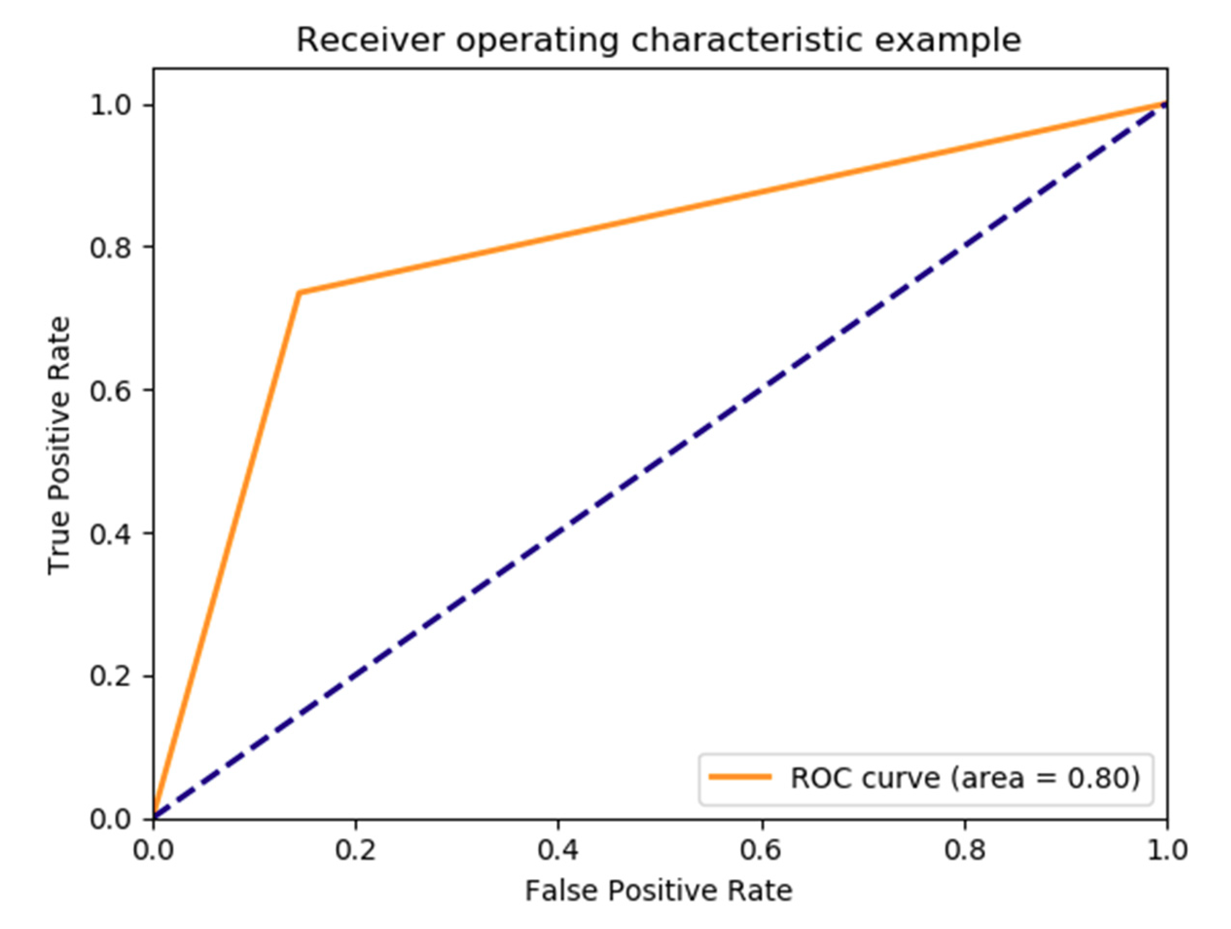
The ROC is a plot of 1—specificity on the x-axis against sensitivity on the y-axis, with each point corresponding to a specific decision threshold. Therefore, the closer the curve is to the top left corner (100% specificity and 100% sensitivity (since the x-axis is 1—sensitivity)) the greater the “overall accuracy of the test” [26]. AUC ROC is a measurement of the area under that curve, which means that it is directly correlated with the overall accuracy of a given classifier.

We measured accuracy and AUC in both holdout (0.25 test size) and 10-fold cross-validation, generated and displayed the ROC curve and confusion matrix, and measured sensitivity, specificity, PPV, NPV, and F1-score.

4.4. Evaluating the Predictability of Features

To evaluate the effect that Overall ROC and Recent ROC had on accuracy, we tested the difference in holdout AUC for the optimal classifiers in each dataset when each of the two ROC features was individually removed and when both were removed.

To test the effectiveness of age and BMI, we measured the increase in AUC holdout when age alone, BMI alone, and both age and BMI were added to the model so far developed.

Since 90% of the patients are white Non-Hispanic people [27], we tested whether filtering by race would have an effect on the accuracy by filtering out all the patients with races other than white Non-Hispanic and seeing if the models built on the remaining data have a higher accuracy.

5. Results

5.1. Result for PoPC Training and Test

The first part of the pipeline, as explained in Section 4.1.3, was to evaluate the effectiveness of each sampling method by running our suite of machine learning methods with each scaling method after sampling the data with a given sampling method.

From Figure 4 and

Table 1. Comparison of data imbalance methods on presence of prostate cancer (PoPC) data, evaluated using the average accuracy (Avg Acc) and average AUC (avg AUC) across all classifiers for the scaling method which achieved the highest average of those two metrics for a given sampling method.

	No Method	CC	RUS	NM1	NM2	NM3
Avg Acc	0.947	0.747	0.780	0.558	0.288	0.841
Avg AUC	0.558	0.774	0.743	0.703	0.587	0.747
	IHT	RENN	ROS	BS1	BS2	ADASYN
Avg Acc	0.417	0.905	0.818	0.823	0.822	0.794
Avg AUC	0.663	0.707	0.735	0.767	0.750	0.743
	SMOTE	SVMSMOTE	SMOTETomek	SMOTEENN
Avg Acc	0.813	0.855	0.812	0.765
Avg AUC	0.742	0.748	0.743	0.765

, it is not entirely clear which sampling method is optimal for PoPC. In general, SVMSMOTE and BS1 could be the best options, being close to the top of the AUC measurements without sacrificing too much in terms of accuracy. It can be seen from Table 1 that SVMSMOTE achieves an average accuracy 0.032 higher than BS1′s, while BS1′s AUC is 0.019 higher than SVMSMOTE’s. As a result, SVMSMOTE was chosen as the sampling method to be used in the remainder of this section.

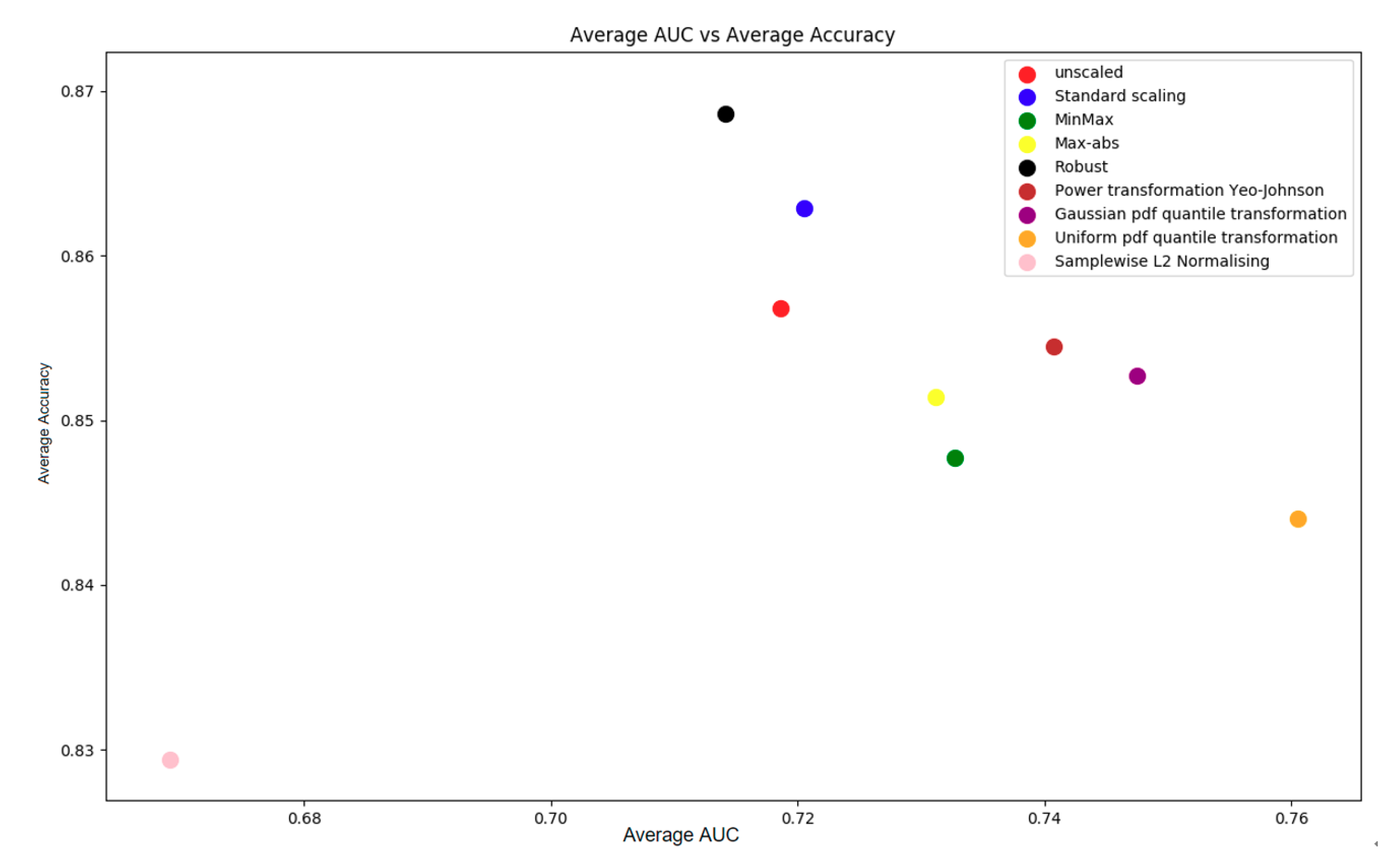
We tested nine scaling methods and calculated the average accuracy and AUC across all classifiers in our suite of machine learning methods (see Section 4.1.4).

It was observed from Figure 5 that a trade-off exists in AUC and accuracy: Robust achieves the highest accuracy with around 0.87 while its AUC is the lowest of any method, whereas the uniform pdf quantile transformation achieves an AUC of over 0.76, with the second lowest accuracy of 0.844. In this study, we chose standard scaling as the method that was used in the analysis process, as both the AUC and accuracy achieved by this method were acceptable.

The evaluations of classifiers are presented in

Table 2. Average accuracy and AUC score for each machine learning algorithm on PoPC training/test.

	KN	SVM2	QD	DT	RF	MLPC	ADA
Holdout accuracy	0.886	0.899	0.916	0.831	0.831	0.850	0.846
Holdout auc-score	0.683	0.653	0.577	0.777	0.772	0.791	0.777
10-fold cross validation accuracy	0.876 (±0.009)	0.894 (±0.013)	0.919 (±0.009)	0.838 (±0.023)	0.835 (±0.024)	0.845 (±0.015)	0.843 (±0.014)
10-fold cross validation auc	0.674 (±0.038)	0.662 (±0.049)	0.575 (±0.049)	0.778 (±0.030)	0.771 (±0.024)	0.771 (±0.037)	0.776 (±0.028)

. In Holdout methods, 25% of the data were used for testing and the rest were used to train the classifiers. The performance of classifiers varies for accuracy and AUC score (Table 2). ADABoost was the best algorithm for this dataset, given that it had the equal best AUC in holdout and is only 0.002 off the best in cross-validation. Its accuracy in both was also no more than 0.076 from the top accuracy, and was higher than that of decision tree, which was the only algorithm with better AUC. Therefore, ADABoost is the machine learning algorithm used for this model in the remaining predictions on PoPC-labelled data.

The ROC curve of the model is presented in Figure 6 and its confusion matrix is demonstrated in

Table 3. Confusion matrix for decision tree on PoPC data training and test.

	Disease Present	Disease Absent
Predicted present	208	725
Predicted absent	75	4285

.

The detailed performance of this model is shown in

Table 4. Specificity, sensitivity, PPV, and NPV for decision tree on PoPC data.

Evaluation	Value
Sensitivity	0.735
Specificity	0.855
PPV	0.223
NPV	0.983
F1	0.342

.

Table 5. AUC and decrease in AUC for optimal classifier on PoPC data when selected features are added or removed.

	AUC	Difference in AUC by Different Feature Set
No exclusion (Same feature set as above model)	0.791	0
Recent ROC excluded	0.767	−0.024
Overall ROC excluded	0.787	−0.004
Overall ROC and Recent ROC excluded	0.774	−0.017
Age added	0.786	−0.005
BMI added	0.792	+0.001
Age and BMI added	0.786	−0.005
Filtered by race	0.785	−0.006

shows the performance of classifiers trained using different feature sets. The addition and exclusion were all based on the original feature set of 6 PSA levels, Overall ROC, and Recent ROC. The AUC were evaluated by holdout instead of cross-validation; thus, there might exist slight differences in the resulting AUC.

Table 5 demonstrates that Overall- ROC and Recent ROC both make contributions to the accuracy of the model thus far developed, with Recent ROC making a greater contribution. In fact, when both of them are excluded, there is less of a decrease in accuracy than when Recent ROC alone is excluded. Age decreased accuracy, while BMI slightly improved it, and adding both together decreased accuracy. Filtering by race had a negative effect on accuracy. Thus, the evaluation of features suggests that the most effective feature set for this model contains only PSA levels, Recent ROC, and BMI.

5.2. Result for PoHRPC Training and Test

To predict high-risk prostate cancer, we used the previously developed pipeline in the last section.

From

Table 6. Average accuracy and AUC score for each machine learning algorithm on PoHRPC training/test.

	KN	SVM2	QD	DT	RF	MLPC	ADA
Holdout accuracy	0.979	0.926	0.930	0.906	0.930	0.905	0.929
Holdout auc-score	0.551	0.674	0.630	0.687	0.653	0.618	0.664
10-fold cross validation accuracy	0.979 (±0.007)	0.925 (±0.011)	0.941 (±0.011)	0.927 (±0.016)	0.915 (±0.028)	0.909 (±0.030)	0.894 (±0.013)
10-fold cross validation auc	0.576 (±0.082)	0.686 (±0.108)	0.617 (±0.098)	0.669 (±0.086)	0.696 (±0.115)	0.675 (±0.114)	0.711 (±0.120)

, we observed that ADABoost had the highest AUC according to cross-validation and the third highest according to holdout. In terms of accuracy, it is within a reasonable margin of all algorithms that are close to it in terms of AUC. Therefore, we used this method for the rest of the evaluation in this section, and in the comparison with other papers at the end of the results section.

The ROC curve for this model is presented in Figure 7 and its confusion matrix achieved by is in

Table 7. Confusion matrix for ADABoost on PoHRPC data training and test.

	Positive	Negative
Predicted positive	28	457
Predicted negative	17	4791

. Note that the confusion matrix is evaluated using holdout instead of cross-validation.

The detailed performance of this model is shown in

Table 8. Specificity, sensitivity, PPV and NPV for ADABoost on PoHRPC data.

Evaluation	Value
Sensitivity	0.62
Specificity	0.913
PPV	0.057
NPV	0.996
F1	0.106

.

Table 9. AUC and decrease in AUC for optimal classifier on PoHRPC data when selected features are added or removed.

	AUC	Difference in AUC by Different Feature Set
No exclusion (Same feature set as above model)	0.673	0
Recent ROC excluded	0.651	−0.022
Overall ROC excluded	0.661	−0.012
Both Overall ROC and Recent ROC excluded	0.643	−0.03
Age added	0.711	+0.038
BMI added	0.688	+0.015
Age and BMI added	0.690	+0.017
Filtered by race	0.669	−0.004

shows the performance of classifiers trained using different feature sets. The addition and exclusion were all based on the original feature set of 6 PSA levels, Overall ROC, and Recent ROC. The AUC were evaluated by holdout instead of cross-validation; thus, there might exist slight differences in the resulting AUC.

It can be seen that exclusion of any of the PSA rate of change variables only decreases the performance of the model. Meanwhile, for additions involving age and BMI, adding only the “age” variable provides the most substantial increase in the performance. Although having BMI as a feature can also provide a better performance than the original model, using age and BMI together cannot produce a result that is comparable to using only age. Finally, filtering by race decreased the accuracy by 0.004, indicating it has a negative effect on accuracy. Therefore, the optimal feature set for this model contains PSA levels, Overall ROC, Recent ROC, and age. Given that without any of these features, the AUC is 0.643 and with all of them the AUC is 0.711, together, they lead to an increase of 6.8% in AUC.

5.3. Comparison of the Results with Related Work

The classifiers discussed in this section are the optimal models for PoPC and PoHRPC as described above (both have SVMSMOTE as their sampling method and standard scaling as their scaling method, with PoHRPC having ADABoost as its machine learning method and PoPC decision tree as its machine learning method), with the results we are reporting on having been calculated when they predicted using the standard feature set of 6 PSA levels, Overall ROC, and Recent ROC.

As shown in

Table 10. Comparison of our results with train/test on the same dataset and testing on a validation set with Shoaibi et al., Roffman et al., and Wang et al.

	PoHRPC (ADABoost)	PoPC (ADABoost)	Wang et al. ANN on Training/Test Set from Same Dataset	Shoaibi et al. Validation	Roffman et al. ANN on Training/Test Set from Same Dataset
Sensitivity	0.62	0.735	0.9996 ± 0.0013	0.955	0.232 (0.195–0.269)
Specificity	0.913	0.855	0.9035 ± 0.0163	0.852	0.894 (0.89–0.897)
NPV	0.996	0.983
PPV	0. 057	0.223			0.265 (0.224–0.306)
Accuracy	0.915 (±0.016)	0.843 (±0.014)	0.9527 ± 0.0079
AUC	0.711 (±0.120)	0.776 (±0.028)	0.9755 ± 0.0073		0.72 (0.70–0.75)

All AUC scores for our data are the maximum achieved by any of the ensemble of classifiers. Training/test accuracy and AUC are measured by 10-fold cross-validation.

, while our optimal classifier on the PoHRPC data set had a specificity of 0.913 which was better than Shoaibi et al.’s of 0.852, our sensitivity of 0.62 was far off theirs of 0.955. Both our study and the study of Roffman et al. achieved poor sensitivity, while the specificity and AUC are decent. Furthermore, we attained a high negative predictive value of 0.996 and a very low positive predictive value of 0.057. What is notable about this is that it indicates, as does the confusion matrix in Table 8, that the major source of error in our predictor was false positives, with us having 457 of those compared to 17 false negatives. This indicates that our imbalance correction method led to a bias towards positive entries in prediction on this data set, relative to the small number of positive entries in the dataset. Nonetheless, Figure 4 indicates that these sampling methods increase the AUC, suggesting we should hold onto them. This is in line with what you would expect from an imbalance correction method, but it does reflect that further optimization needs to be done, especially as false positives are currently a problem with PSA tests [5].

Table 10 demonstrates a tendency of Roffman et al.’s predictor and our two predictors, both of which predicted on imbalanced datasets, performing worse than Wang et al.’s, which predicted on a balanced dataset. Of the four of these predictors (our two predictors, Roffamn et al.’s, and Wang et al.’s) Wang et al.’s dataset had a positive percentage of 50.95%, while PoHRPC had 0.89%, PoPC had 5.34%, and Roffman et al.’s had 1.67%. Wang et al.’s predictor performed the best in terms of every metric shared between all the predictors aside from specificity, with its specificity being 0.0095 less than that of our PoHRPC predictor. This is a negligible difference. Its sensitivity of 0.966 was 0.2366 higher than the next highest sensitivity of the predictors, which was our PoPC predictor with 0.735. Its accuracy of 0.9527 was 0.0377 higher than the next highest, which was our PoHRPC predictor with 0.915. Its AUC was higher than the next highest (our PoPC predictor with 0.776) by 0.1995.

Nonetheless, Shoaibi et al.’s study is a counter-example to this trend, demonstrating a high sensitivity despite predicting on imbalanced data (recall that they too predicted high-risk prostate cancer in the NCI PLCO data set). This shows that it is possible to predict accurately on imbalanced data, which Roffman et al.’s and our predictors failed to do.

6. Discussion and Conclusions

Our evaluation suggests that, for the predictors we have, rate of change does have a positive effect on accuracy, given that Recent ROC contributed 0.024 to the AUC on PoPC, and both variables together contributed 0.03 to the AUC on PoHRPC. Including age in the features set led to a further increase of 0.038 in AUC. Therefore, adding rate of change of PSA variables and age to the feature set of a machine learning predictor for prostate cancer led to an increase of 6.8% in AUC compared to the AUC generated by predicting with PSA levels alone on PoHRPC-labelled data.

Although there are certain differences that exist in the performance between our model and Shoaibi et al.’s model, our model and pipeline can be built easily with less requirement of the input data, and for researchers with no professional statistical modelling experience, our model can be easier to understand and implement, and the result we have achieved can provide a baseline for other studies with similar purpose. Furthermore, the pipeline we have developed can be used as a guide for future studies on the PLCO dataset.

Our models’ low PPV values indicate that our choice of an imbalance correction method could be further investigated. The effect of imbalance correction should be measured by testing the variance of attributes like sensitivity, specificity, NPV and PPV with changing methods. Furthermore, the focus should be on lowering the rate of false positives that currently occur when we use imbalance correction methods. A broad range of methods should be tested, including those in the latest literature. An example of such a method is Ebenuwa et al.’s variance ranking attributes selection technique [18].

Advanced machine learning methods coupled with feature engineering and addition of more features improve prediction models [28,29]. A clear one, as mentioned earlier, is using the ratio of free:total PSA [3], but another option is measurement of androgen and estrogen steroids, since the role of these hormones are acknowledged in other cancer-types [30]. There is research suggesting correlations between these steroids and prostate cancer, such as decreasing androgens and increasing estrogen increasing the likelihood of prostate cancer. When different kinds of estrogens are distinguished between, however, the picture becomes more complicated as activation of the classical estradiol receptors (α and β) have various effects on prostate cancer progression which, due to the sometimes contradictory nature of the results and the present insufficiency of our models of prostate cancer and the receptors involved in it, makes the role of estrogens (that is, whether they increase or decrease the spread of prostate cancer) unclear [31,32]. Machine learning is therefore an area in which the correlations which we believe exist can be used for prediction in clinical practice before more sophisticated models have been developed.

References

- U.S. Preventive Services Task Force. Final Update Summary: Prostate Cancer: Screening; U.S. Preventive Services Task Force: Rockville, MD, USA, 2018. [Google Scholar]
- Wang, G.; Teoh, J.Y.; Choi, K. Diagnosis of prostate cancer in a Chinese population by using machine learning methods. In Proceedings of the 2018 40th Annual International Conference of the IEEE Engineering in Medicine and Biology Society (EMBC), Honolulu, HI, USA, 17–21 July 2018. [Google Scholar]
- Prostate-Specific Antigen (PSA) Test. [4/10/2019]. Available online: https://www.cancer.gov/types/prostate/psa-fact-sheet (accessed on 8 June 2019).
- Martin, R.M.; Donovan, J.L.; Turner, E.L.; Metcalfe, C.; Young, G.J.; Walsh, E.I.; Lane, J.A.; Noble, S.; Oliver, S.E.; Evans, S.; et al. Effect of a low-intensity PSA-based screening intervention on prostate cancer mortality: The CAP randomized clinical trialeffect of 1-time PSA screening on prostate cancer mortality effect of 1-time PSA screening on prostate cancer mortality. JAMA 2018, 319, 883–895. [Google Scholar] [CrossRef] [PubMed]
- Roland, M.; Neal, D.; Buckley, R. What should doctors say to men asking for a PSA test? BMJ 2018, 362, k3702. [Google Scholar] [CrossRef]
- Moyer, V.A.; U.S. Preventive Services Task Force. Screening for prostate cancer: U.S. Preventive services task force recommendation statement. Ann. Intern. Med. 2012, 157, 120–134. [Google Scholar] [PubMed]
- Auvinen, A.; Hakama, M. Cancer Screening: Theory and Applications. In International Encyclopedia of Public Health, 2nd ed.; Quah, S.R., Ed.; Academic Press: Oxford, UK, 2017; pp. 389–405. [Google Scholar]
- Negoita, S.; Feuer, E.J.; Mariotto, A.; Cronin, K.A.; Petkov, V.I.; Hussey, S.K.; Bernard, V.; Henley, S.J.; Anderson, R.N.; Fedewa, S. Annual report to the Nation on the status of cancer, part II: Recent changes in prostate cancer trends and disease characteristics. Cancer 2018, 124, 2801–2814. [Google Scholar] [CrossRef] [PubMed]
- Ahmed, H.U.; Kirkham, A.; Arya, M.; Illing, R.; Freeman, A.; Allen, C.; Emberton, M. Is it time to consider a role for MRI before prostate biopsy? Nat. Rev. Clin. Oncol. 2009, 6, 197. [Google Scholar] [CrossRef] [PubMed]
- Lapa, P.; Goncales, I.; Rundo, L.; Casteli, M. Semantic learning machine improves the CNN-Based detection of prostate cancer in non-contrast-enhanced MRI. In Proceedings of the ACM Genetic and Evolutionary Computation Conference Companion, Prague, Czechia, 13–17 July 2019. [Google Scholar]
- Rundo, L.; Militello, C.; Russo, G.; Garufi, A.; Vitabile, S.; Gilardi, M.C.; Mauri, G. Automated prostate gland segmentation based on an unsupervised fuzzy C-means clustering technique using multispectral T1w and T2w MR imaging. Information 2017, 8, 49. [Google Scholar] [CrossRef]
- Shoaibi, A.; Rao, G.A.; Cai, B.; Rawl, J.; Haddock, K.S.; Hebert, J.R. Prostate specific antigen-growth curve model to predict high-risk prostate cancer. Prostate 2017, 77, 173–184. [Google Scholar] [CrossRef]
- Roffman, D.A.; Hart, G.R.; Leapman, M.S.; Yu, J.B.; Guo, F.L.; Deng, J. Development and validation of a multiparameterized artificial neural network for prostate cancer risk prediction and stratification. JCO Clin. Cancer Inf. 2018, 2, 1–10. [Google Scholar] [CrossRef]
- Lecarpentier, J.; Silvestri, V.; Kuchenbaecher, K.B.; Barrowdale, D.; Dennis, J.; McGuffog, L.; Soucy, P.; Leslie, G.; Rizzolo, P.; Navazio, A.S.; et al. Prediction of breast and prostate cancer risks in male BRCA1 and BRCA2 mutation carriers using polygenic risk scores. J. Clin. Oncol. 2017, 35, 2240. [Google Scholar]
- Vickers, A.J.; Cronin, A.M.; Aus, G.; Pihl, C.-G.; Becker, C.; Pettersson, K.; Scardino, P.T.; Hugosson, J.; Lilja, H. A panel of kallikrein markers can reduce unnecessary biopsy for prostate cancer: data from the European Randomized Study of Prostate Cancer Screening in Göteborg, Sweden. BMC Med. 2008, 6, 19. [Google Scholar] [CrossRef]
- Chang, A.J.; Autio, K.A.; Roach, M., 3rd; Scher, H.I. High-risk prostate cancer-classification and therapy. Nat. Rev. Clin. Oncol. 2014, 11, 308–323. [Google Scholar] [CrossRef] [PubMed]
- Pedregosa, F.; Varoquaux, G.; Gramfort, A.; Michael, V.; Thirion, B.; Grisel, O.; Blondel, M.; Prettenhofer, P.; Weiss, R.; Dubourg, V.; et al. Scikit-learn: Machine Learning in Python. JMLR 2011, 12, 2825–2830. [Google Scholar]
- Ebenuwa, S.H.; Sharif, M.S.; Alazab, M.; Al-nemrat, A. Variance ranking attributes selection techniques for binary classification problem in imbalance data. IEEE Access 2019, 7, 24649–24666. [Google Scholar] [CrossRef]
- Imbalanced-Learn. 2016. Available online: https://imbalanced-learn.readthedocs.io/en/stable/index.html (accessed on 10 June 2019).
- Chawla, N.V.; Bowyer, K.W.; Hall, L.O.; Kegelmeyer, W.P. SMOTE: synthetic minority over-sampling technique. J. Artif. Intell. Res. 2002, 16, 321–357. [Google Scholar] [CrossRef]
- Han, H.; Wang, W.-Y.; Mao, B.-H. Borderline-SMOTE: A New Over-Sampling Method in Imbalanced Data Sets Learning. In International Conference on Intelligent Computing; Springer: Berlin/Heidelberg, Germany, 2005. [Google Scholar]
- Jeatrakul, P.; Wong, K.W.; Fung, C.C. Classification of imbalanced data by combining the complementary neural network and SMOTE algorithm. In International Conference on Neural Information Processing; Springer: Berlin/Heidelberg, Germany, 2010. [Google Scholar]
- Tang, Y.; Zhang, Y.-Q.; Chawla, N.V.; Krasser, S. SVMs modeling for highly imbalanced classification. IEEE Trans. Syst. Man Cybern. Part B 2008, 39, 281–288. [Google Scholar] [CrossRef]
- Santos, M.; Soares, J.P.; Abreu, P.H.; Araujo, H.; Santos, J. Cross-validation for imbalanced datasets: Avoiding overoptimistic and overfitting approaches. IEEE Comput. Intell. Mag. 2018, 13, 59–76. [Google Scholar] [CrossRef]
- Brownlee, J. How to Train. a Final Machine Learning Model. 2017. Available online: https://machinelearningmastery.com/train-final-machine-learning-model/ (accessed on 26 May 2019).
- ROC Curve Analysis. 2016. Available online: https://www.medcalc.org/manual/roc-curves.php (accessed on 26 May 2019).
- Zhu, C.S.; Pinsky, P.F.; Kramer, B.S.; Prorok, P.C.; Purdue, M.P.; Berg, C.D.; Gohagan, J.K. The prostate, lung, colorectal, and ovarian cancer screening trial and its associated research resource. J. Natl. Cancer Inst. 2013, 105, 1684–1693. [Google Scholar] [CrossRef]
- Khushi, M.; Dean, I.M.; Teber, E.T.; Chircop, M.; Arhtur, J.W.; Flores-Rodriguez, N. Automated classification and characterization of the mitotic spindle following knockdown of a mitosis-related protein. BMC Bioinform. 2017, 18, 566. [Google Scholar] [CrossRef]
- Khushi, M.; Napier, C.E.; Smyth, C.M.; Reddel, R.R.; Arhtur, J.W. MatCol: A tool to measure fluorescence signal colocalisation in biological systems. Sci. Rep. 2017, 7, 8879. [Google Scholar] [CrossRef]
- Khushi, M.; Clarke, C.L.; Graham, J.D. Bioinformatic analysis of cis-regulatory interactions between progesterone and estrogen receptors in breast cancer. Peer J. 2014, 2, e654. [Google Scholar] [CrossRef] [Green Version]
- Di Zazzo, E.; Galasso, G.; Giovannelli, P.; Di Donato, M.; Di Santi, A.; Cernera, G.; Rossi, V.; Abbondanza, C.; Moncharmont, B.; Sinisi, A.A.; et al. Prostate cancer stem cells: the role of androgen and estrogen receptors. Oncotarget 2016, 7, 193–208. [Google Scholar] [CrossRef] [PubMed]
- Di Zazzo, E.; Galasso, G.; Giovannelli, P.; Di Donato, M.; Castoria, G. Estrogens and their receptors in prostate cancer: Therapeutic implications. Front. Oncol. 2018, 8, 2. [Google Scholar] [CrossRef] [PubMed]
Figure 1.
Population of National Cancer Institute’s Prostate, Lung, Colorectal, and Ovarian Screening Trial (NCI PLCO) dataset upon different inclusion/exclusion criteria and the positive instances been selected for analysis.
Figure 2.
Segmentation of NCI PLCO into no cancer, low-risk prostate cancer, and high-risk prostate cancer.
Figure 3.
The whole process of the analysis.
Figure 4.
Average area under the curve (AUC) vs. average accuracy across all classifiers for each sampling method on optimally scaled PoPC data.
Figure 5.
Average AUC for the ensemble of algorithms on each scaling method vs. average accuracy for the ensemble of algorithms on each scaling method on PoPC data.
Figure 6.
Receiver operating characteristic curve for decision tree on PoPC data.
Figure 7.
Receiver operating characteristic curve for ADABoost on PoHRPC data.