On-Demand Processing of Data Cubes from Satellite Image Collections with the gdalcubes Library


Institute for Geoinformatics, University of Münster, Heisenbergstraße 2, 48149 Münster, Germany
*
Author to whom correspondence should be addressed.
Data 2019, 4(3), 92; https://0-doi-org.brum.beds.ac.uk/10.3390/data4030092
Submission received: 29 May 2019
/
Revised: 25 June 2019
/
Accepted: 26 June 2019
/
Published: 28 June 2019
(This article belongs to the Special Issue Earth Observation Data Cubes)
Abstract
:Earth observation data cubes are increasingly used as a data structure to make large collections of satellite images easily accessible to scientists. They hide complexities in the data such that data users can concentrate on the analysis rather than on data management. However, the construction of data cubes is not trivial and involves decisions that must be taken with regard to any particular analyses. This paper proposes on-demand data cubes, which are constructed on the fly when data users process the data. We introduce the open-source C++ library and R package gdalcubes for the construction and processing of on-demand data cubes from satellite image collections, and show how it supports interactive method development workflows where data users can initially try methods on small subsamples before running analyses on high resolution and/or large areas. Two study cases, one on processing Sentinel-2 time series and the other on combining vegetation, land surface temperature, and precipitation data, demonstrate and evaluate this implementation. While results suggest that on-demand data cubes implemented in gdalcubes support interactivity and allow for combining multiple data products, the speed-up effect also strongly depends on how original data products are organized. The potential for cloud deployment is discussed.
1. Introduction
Recent open data policies from governments and space agencies have made large collections of Earth observation data freely accessible to everyone. Scientists nowadays have data to analyze environmental phenomena on a global scale. For example, the fleet of Sentinel satellites from the European Copernicus program [1] is continuously measuring variables on the Earth’s surface and in the atmosphere, producing terabytes of data every day. At the same time, the structure of satellite imagery is inherently complex [2,3]. Images spatially overlap, may have different spatial resolutions for different spectral bands, produce an irregular time series e.g., depending on latitude and swath, and naturally use different map projections for images from different parts of the world. This becomes even more complicated when data from multiple sensors and satellites must be combined as pixels rarely align in space and time, and the data formats in which images are distributed also vary.
Earth observation (EO) data cubes [4,5] offer a simple and intuitive interface to access satellite-based EO data by hiding complexities for data users, who can then concentrate on developing new methods instead of organizing the data. Due to its simplicity as a regular multidimensional array [6], data cubes facilitate applications based on many images such as time series and even multi-sensor analyses. At the same time, they simplify computational scalability because many problems can be parallelized over smaller sub-cubes (chunks). For instance, time series analyses often process individual pixel time series independently and a data cube representation hence makes parallelization straightforward.
Fortunately, there is a wide available array of technology that works with Earth observation imagery and data cubes. The Geospatial Data Abstraction Library (GDAL) [7] is an open source software library that is used on a large scale by the Earth observation community because it can read all data formats needed, and has high-performance routines for image warping (regridding an image to a grid in another coordinate reference system) and subsampling (reading an image at a lower resolution). However, it has no understanding of the time series of images, nor of temporal resampling or aggregation.
Database systems such has Rasdaman [8] and SciDB [9,10] have been used to store satellite image time series as multidimensional arrays. These systems follow traditional databases in the sense that they can organize the data storage, provide higher level query languages for create, read, update, and delete operations, as well as managing concurrent data access. The query languages of both mentioned systems also come with some basic data cube-oriented operations like aggregations over dimensions. However, array databases are rather infrastructure-oriented. They require a substantial effort in preparing and setting up the infrastructure, and databases typically require data ingestion, meaning that they maintain a full copy of the original data.
The Open Data Cube project (ODC) [11] provides open-source tools to set up infrastructures providing access to satellite imagery as data cubes. The implementation is written in Python and supports simple image indexing without the need of an additional copy. Numerous instances like the Australian data cube [4] or the Swiss data cube [5] are already running or are under development and demonstrate the impact of the technology with the vision to “support . . . the United Nations Sustainable Development Goals (UN-SDG) and the Paris and Sendai Agreements” [11].
Google Earth Engine (GEE) [3] even provides access to global satellite imagery including the complete Sentinel, Landsat, and MODIS collections. GEE is a cloud platform that brings the computing power of the Google cloud directly to data users by providing an easy-to-use web interface for processing data in JavaScript. The success of GEE can be explained not only by the availability of data, computing power, and an accessible user interface but also by the interactivity it provides for incremental method development. Scripts are only evaluated for the pixels that are actually visible on the interactive map, meaning that computation times are highly reduced by sub-sampling the data. GEE does not store image data as a data cube but provides cube-like operations, such as reduction over space and time.
Both, ODC and GEE provide Python clients but lack interfaces to other languages used in data science such as R or Julia. Additionally, the Pangeo project [12] is built around the Python ecosystem, including the packages xarray [13] and dask [14]. For data users working with R [15], two packages aiming at processing potentially large amounts of raster data are raster [16] and stars [17]. While raster represents datasets as two- or three-dimensional only and hence requires some custom handling of multispectral image time series, the stars package implements raster and vector data cubes with an arbitrary number of dimensions, and follows the approach of GEE by computing results only for pixels that are actually plotted, whereas raster always works with full resolution data. However, the stars package at the moment cannot create raster data cubes from spatially tiled imagery, where images come e.g., from different zones of the Universal Transverse Mercator (UTM) system.
Most of the presented tools to process data cubes including Rasdaman, SciDB, xarray, and stars assume that the data already come as a data cube. However, satellite Earth observation datasets are rather a collection of images (Section 2) and generic, cross language tools to construct data cubes from image collections are currently missing. In this paper, we propose on-demand data cubes as an interface on how data users can process EO imagery, supporting interactive analyses where data cubes are constructed on-the-fly and properties of the cube including the spatiotemporal resolution, spatial and temporal extent, resampling or aggregation strategy, and target spatial reference system can be user-defined. We present the gdalcubes C++ library and corresponding R package as a generic implementation of the construction of on-demand data cubes.
The remainder of the paper is organized as follows. Section 2 introduces the concept of on-demand data cubes for satellite image collections and presents our implementation as the gdalcubes software library. Two study cases on Sentinel-2 time series processing and constructing multi-sensor data cubes from precipitation, vegetation, and land surface temperature data evaluate the approach in Section 3, after which Section 4 and Section 5 discuss the results and conclude the paper.
2. Representing Satellite Imagery as On-Demand Data Cubes with gdalcubes
2.1. Data Cubes vs. Image Collections
Earth observation data cubes are commonly defined as multidimensional arrays [6] with dimensions for space and time. We concentrate on the representation of multi-spectral satellite image time series as a data cube and here we therefore narrow it down to the following definition of a regular, dense raster data cube.
Definition 1.
A regular, dense raster data cube is a four-dimensional array with dimensions x (longitude or easting), y (latitude or northing), time, and bands with the following properties:
- (i)
- Spatial dimensions refer to a single spatial reference system (SRS);
- (ii)
- Cells of a data cube have a constant spatial size (with regard to the cube’s SRS);
- (iii)
- The spatial reference is defined by a simple offset and the cell size per axis, i.e., the cube axes are aligned with the SRS axes;
- (iv)
- Cells of a data cube have a constant temporal duration, defined by an integer number and a date or time unit (years, months, days, hours, minutes, or seconds);
- (v)
- The temporal reference is defined by a simple start date/time and the temporal duration of cells;
- (vi)
- For every combination of dimensions, a cell has a single, scalar (real) attribute value.
This specific data cube type has a number of limitations and other definitions are more general (see e.g., [18,19,20]). However we will show how our implementation in the gdalcubes library allows the construction of such cubes from different data sources in Section 3, and help solve a wide range of problems.
As discussed in Section 1, satellite imagery is inherently complex and irregular. For example, a single Sentinel-2 image has different pixel sizes for different spectral bands. Multiple Sentinel-2 images may spatially overlap, and use different map projections (UTM zones). Furthermore, although the regular revisit time for Sentinel-2 data is five days (including both satellites), the temporal differences between images from adjacent orbits might be less than five days, leading to an irregular time series as soon as analyses cover larger spatial regions. Space agencies and cloud computing providers including new platforms such as the Copernicus Data and Information Access Services (DIASes), currently do not provide a data cube access to the data. Except for some platforms discussed in Section 1, including Google Earth Engine, the starting point for data users is often just the files, whether in the cloud or on a local computer. To efficiently build on-demand data cubes from irregularly aligned imagery, we define a data structure for image collections, representing how satellite-based Earth observation data products are distributed to the users.
Definition 2.
An image collection is a set of n images, where images contain m variables or spectral bands. Band data from one image share a common spatial footprint, acquisition date/time, and spatial reference system but may have different pixel sizes. Technically, the data of bands may come from one or more files, depending on the organization of a particular data product.
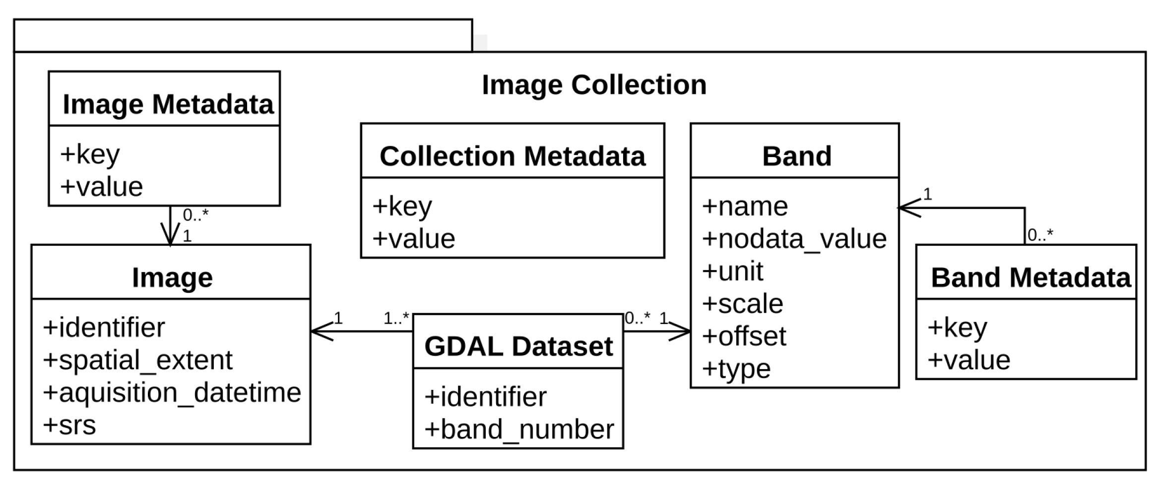
Obviously, images in a collection should come from the same data product, i.e., measurement values must be comparable. Figure 1 illustrates how image collections are implemented in gdalcubes.
2.2. Constructing User-Defined Data Cubes from Image Collections
Constructing data cubes involves some decisions that may include loss of information. These include the selection of the spatial reference system, the resolution in space and time, the area and time range of interest, and a resampling algorithm. Decisions may or may not be appropriate for particular analyses and we therefore delay the construction of the data cube until data must actually be read in the analysis. The idea is similar to how Google Earth Engine works: Users write their analysis and independently select parameters, like the area of interest and the resolution. We define a target cube with a data cube view, an object that defines the cube “geometry”, and how it is created, including the target cube’s:
- Spatial reference system;
- Spatiotemporal extent;
- Spatial size and temporal duration of cells (resolution);
- Spatial image resampling method, and;
- Temporal aggregation method.
The spatial resampling algorithm is applied when reprojecting, cropping, and/or resizing pixels of one image. The temporal aggregation method specifies how pixel values from multiple images that are covered by the same cell in the target data cube are combined. For example, if a data cube pixel has a temporal duration of one month, values from multiple images need to be combined, e.g., by averaging the five-daily values covered by a particular month. Similar to [21], who formalize a topological map algebra for analyzing irregular spatiotemporal datasets including satellite image collections, this allows to adapt the temporal granularity to the specific needs, and to make this explicit.
To lower memory requirements and to read and process data in parallel for larger cubes, we divide a target data cube into smaller chunks, whose spatiotemporal size can be specified by users and can be tuned to improve the performance of particular analyses. A chunk always contains data from all bands. Below, we summarize the algorithm to read a data cube chunk, given an image collection and a data cube view. The algorithm returns an in-memory four-dimensional dense array.
- Allocate and initialize an in-memory chunk buffer for the resulting chunk data (a four-dimensional bands, t, y, x array);
- Find all images of the collection that intersect with the spatiotemporal extent of the chunk;
- For all images found:
- 3.1.
- Crop, reproject, and resample according to the spatiotemporal extent of the chunk and the data cube view and store the result as an in-memory three-dimensional (bands, y, x) array;
- 3.2.
- Copy the result to the chunk buffer at the correct temporal slice. If the chunk buffer already contains values at the target position, update a pixel-wise aggregator (e.g., mean, median, min., max.) to combine pixel values from multiple images which are written to the same cell in the data cube.
- Finalize the pixel-wise aggregator if needed (e.g., divide pixel values by n for mean aggregation).
In the case of median aggregation, non-missing values from all contributing images are collected in an additional dynamically sized per-pixel buffer before the median can be calculated in the final step.
2.3. Data Cube Operations
Since data cubes as defined in this paper are simple multidimensional arrays, it is easy to express higher-level operators that take one (or more) data cubes as input and produce one data cube as a result. Examples include reduction over dimensions, applying arithmetic expressions on pixels, or focal window operations like image convolution. Table 1 lists some operations that are already implemented in gdalcubes.
These operations can be chained, essentially constructing a directed acyclic graph of operations. The graph allows reordering operations in order to optimize computations and minimize data reads. Furthermore, chunks of data cubes can be processed in parallel.
2.4. The gdalcubes Library
The open-source C++ library and R package gdalcubes implement the concept of on-demand raster data cubes described above. The library includes data structures for image collections, raster data cubes, data cube views, and includes some high-level data cube operations (see Table 1). It uses the Geospatial Data Abstraction Library (GDAL) [7] to read and warp images, the netCDF C library [22] to export data cubes as files, SQLite [23] to store image collection indexes on disk, and libcurl [24] to perform HTTP requests. Additionaly it includes the external libraries tinyexpr [25] to parse and evaluate C expressions at runtime, date [26] for a modern C++ datetime approach, a tiny-process-library [27] to start external processes, and json [28] to parse and convert C++ objects from/to json. In the following, we focus on the description of the R package which simply wraps classes and functions from the underlying C++ library but does not add important features. The R package is available from the Comprehensive R Archive Network (CRAN)1.
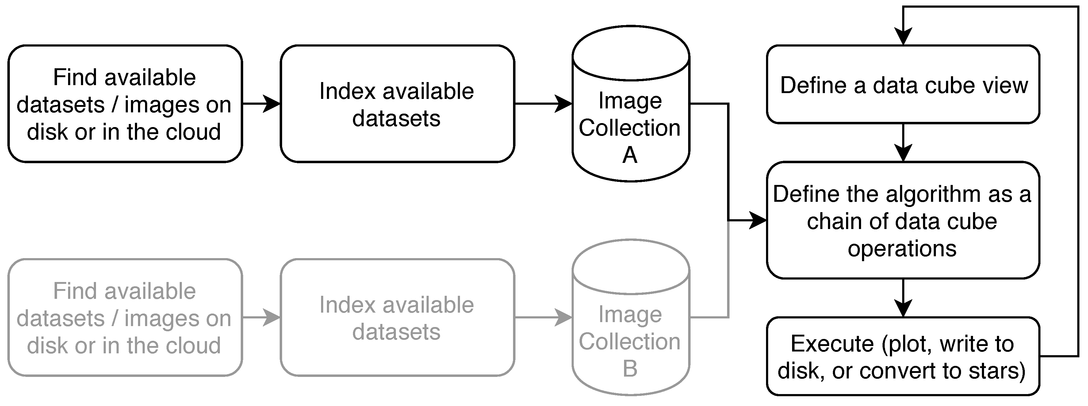
Figure 2 illustrates the basic workflow of how the package is used. At first, available images must be indexed to build an image collection. The image collection stores the spatial extent, the spatial reference system, the acquisition time of images, how bands relate to individual datasets or files, and where the image data can be found. The resulting image collection is a simple SQLite single file database with tables for images, bands, datasets, and metadata according to Figure 1.
Since we use GDAL to read image data, datasets can point to anything that GDAL can read, including local or remote files, object storage from cloud providers, sub-datasets in hierarchical file formats, compressed files, or even databases. GDAL dataset identifiers simply tell GDAL where to find and how to read the image data. The data structure with a one-to-many relationship between images and GDAL datasets and a one-to-many relationship between GDAL datasets and bands brings maximum flexibility in how the input collections can be organized. Images can be composed from a single file containing all bands (e.g., MODIS), from many files where one file contains data for one band (e.g., Landsat 8), or even from many files where files store some of the bands (e.g., grouped by spatial resolution). Again, files here are not limited to local files but refer to anything that GDAL can read. We chose SQLite for its portability and simplicity, relieving users from the need to run an additional database. To support fast spatiotemporal range selection and filtering, the image table contains indexes on the spatial extent and the acquisition date/time.
However, due to the variety of available EO products and its diverse formats and naming conventions, it is not trivial to extract all the information automatically. We abstract from specific products by defining collection formats for specific EO products. The package comes with a set of predefined formats including some Sentinel, Landsat, and MODIS data products. Further formats can be either user-defined or downloaded from a dedicated GitHub repository2, where new formats will be continuously added. Internally, the collection formats are JSON files following a rather simple format that includes a description of the collection’s bands and a few regular expressions on how to extract the needed fields, e.g., from a granule’s file name.
After one or more image collections have been created, the typical workflow (Figure 2) is to define a data cube view that includes the area and time of interest, the target spatial reference system, and the spatiotemporal resolution, then define operations on the data cube, and finally plot or write the result to disk. These steps are typically repeated, where users refine the data cube view or the operations carried out on retrieved cubes. This fits well to incremental method development because users can try their methods on coarse resolution and/or a spatiotemporal extent first, before scaling the analysis to large regions and/or high resolution.
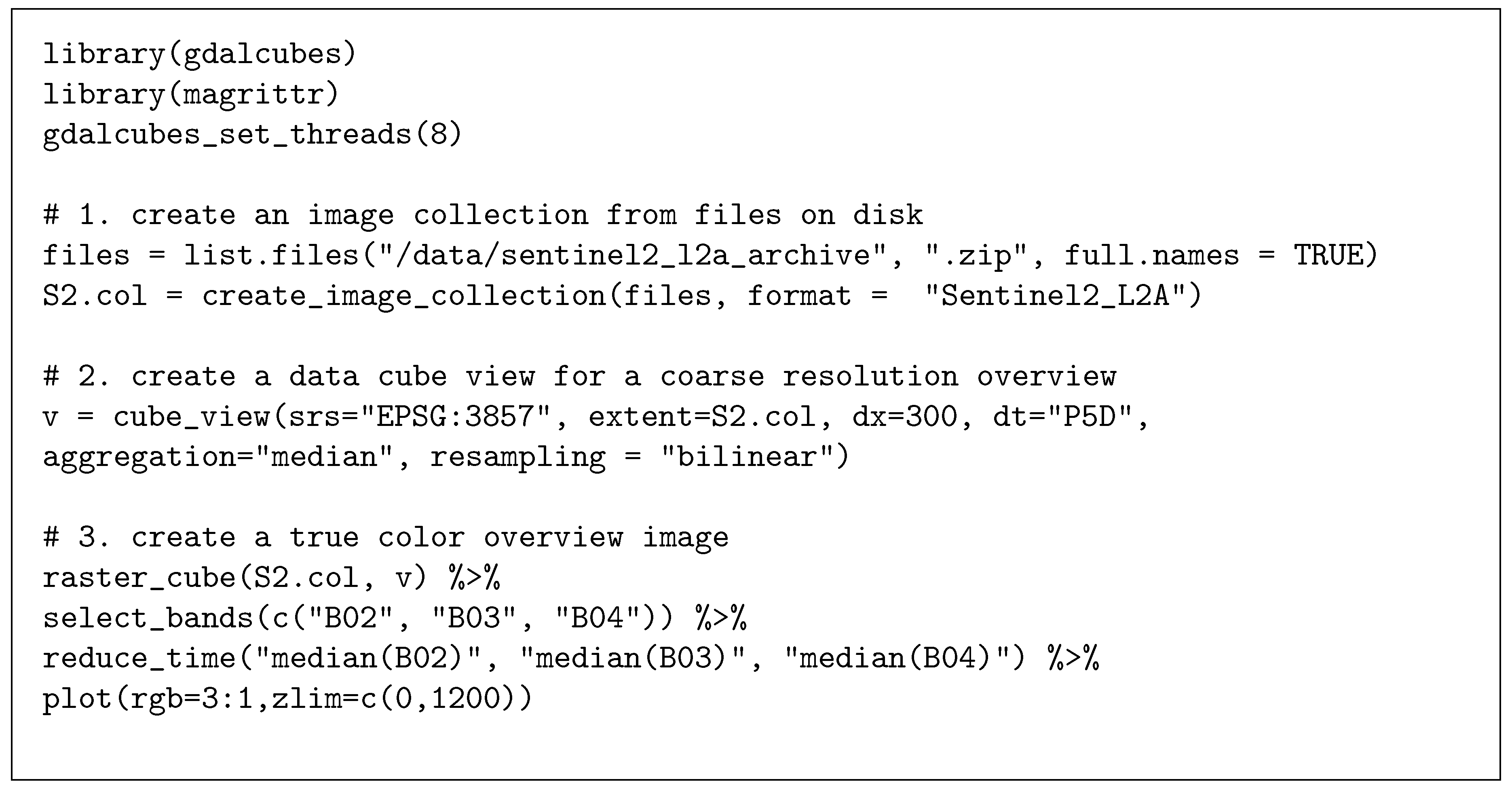
The workflow can also be identified in Figure 3, showing a minimal example R script to derive a preview image from a collection of Sentinel-2 Level 2A images by applying a median reducer over the visible bands at a 300 m spatial resolution. We first create an image collection with create_image_collection(), indexing available files on the local disk, then define a data cube view with cube_view(), and create the cube with raster_cube(). Calling this operation will however neither start any expensive computations nor read any pixel data from disk. Instead, the function immediately returns a proxy object that can be passed to data cube operations. We subset available bands of the data cube by calling select_bands() and apply a median reducer over time with reduce_time(). These functions also return proxy objects, containing the complete chain of operations and the dimensions of the resulting cube. Expressions passed as strings to data cube operations directly translate to C++ functions. In this case, the median reduction is fully implemented in C++ and does not need to call any R functions on the data. The plot() call finally executes the chain of operations and starts actual computations and data reads. The advantage of such a lazy evaluation is that no intermediate results must be written to disk but can be directly streamed to the next operation so that the order of operations can be optimized. In an example with 102 images from three adjacent grid tiles (summing to approximately 90 gigabytes), stored as original ZIP archives as downloaded from the Copernicus Open Access Hub [29] (see also Section 3, where we use the same dataset in the second study case), computations take around 40 s on a personal laptop with a quad-core CPU, 16 GB main memory, and a solid state disk drive. The resulting image is shown in Figure 4. The complete script has less than 20 lines of code and if users want to apply the same operation at a higher resolution, possibly for a different spatial extent and time range, only parameters that define the data cube view must be changed.
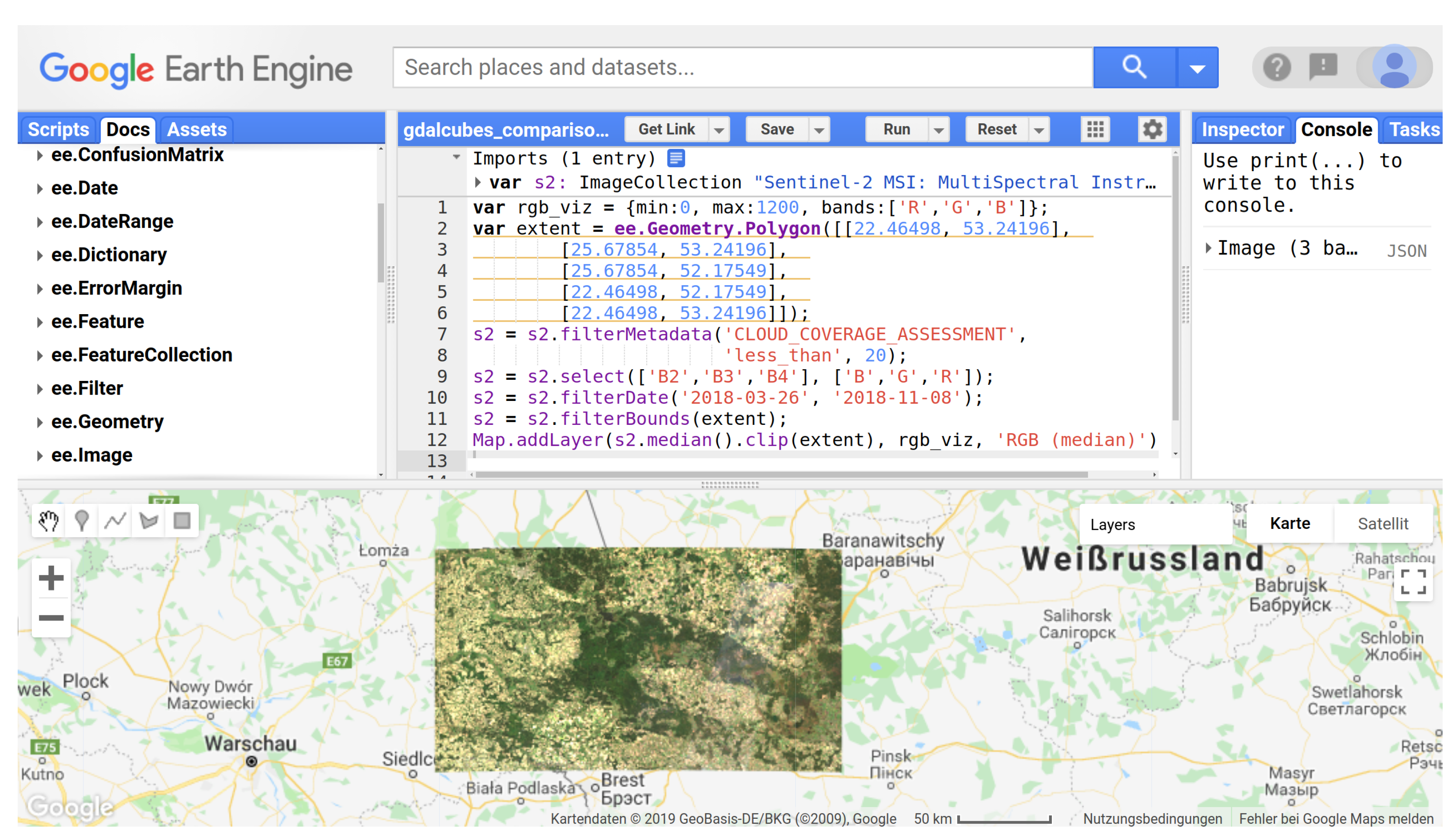
Figure 5 shows a Google Earth Engine (GEE) script for applying a median (time) reduction over the same study region. The results are very similar but not identical on pixel level because of a few different images being used and because GEE reduced the entire image collections whereas gdalcubes creates data cubes with regular temporal resolution, which involves aggregating values from multiple images before applying the reducer.
3. Study Cases
We now demonstrate and evaluate the R package implementation in two study cases. The first study case focuses on demonstrating how gdalcubes can be used to combine different data products. The second study case processes Sentinel-2 time series and evaluates the scalability of computation times as a function of the resolution of the data cube view and the number of CPUs used. All computation time measurements have been performed on a Dell PowerEdge R815 Server with 4 AMD Opteron 6376 CPUs, summing to 64 CPU cores in total and 256 GB of main memory.
3.1. Constructing a Multi-Sensor Data Cube from Precipitation, Vegetation Data, and Land Surface Temperature Data
In this case study, we build a multi-sensor data cube including 16-daily vegetation index data from the Moderate-resolution Imaging Spectroradiometer (MODIS) product MOD13A23, daily land surface temperature data from the MODIS product MOD11A14, and daily precipitation data from the Global Precipitation Measurement mission (GPM) product IMERG5 (using the daily accumulated, final-run product). Table 2 summarizes some important properties of the datasets used in this study case. Combining data from such sensors including meteorological and optical measurements is an important step in analyzing statistical dependencies between environmental phenomena. In this case, the combined resulting data cube can, for example, be used to study the resistance of vegetation against heat or drought periods.
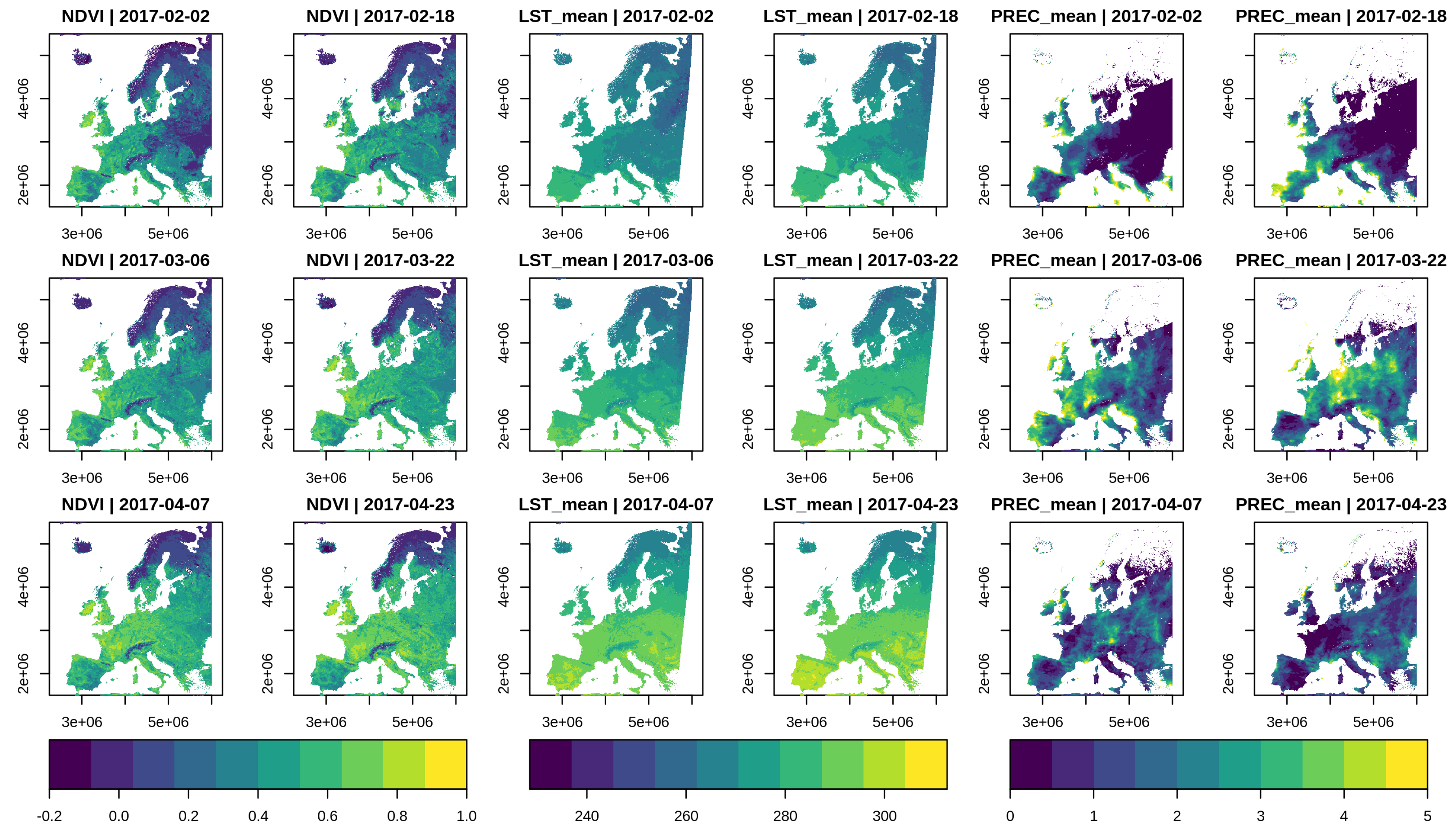
The script to build a combined data cube is shown in Figure 6. We first create a common data cube view, covering Europe from the beginning of 2014 to the end of 2018 at a 10 km spatial and daily temporal resolution. Then, we create three separate raster data cubes and apply some individual operations, e.g., to compute 30-day precipitation means from daily measurements. We then combine the cubes using two calls to the join_bands() function, which collects the bands from two identically shaped data cubes. Since the MOD13A2 product covers land areas only, we ignore any pixels in the combined cube without vegetation data by calling filter_predicate(). Expressions passed to the apply_pixel and filter_predicate functions are translated to C++ functions, with iif denoting a simple one line if-else statement. Finally, we export the cube as a netCDF file. Figure 7 shows a resulting temporal subset of a cube derived at a 10 km spatial resolution. Computation times to execute the script varied between 40 and 240 min on a 50 km and 1 km spatial resolution respectively, meaning that by reducing the number of pixels in the target data cube by a factor of 2500, we could reduce computation times by a factor of 6. In this case, data users would additionally need to reduce the area and/or time range of interest to try out methods and get interactive results within a few minutes.
3.2. Processing Sentinel-2 Time Series
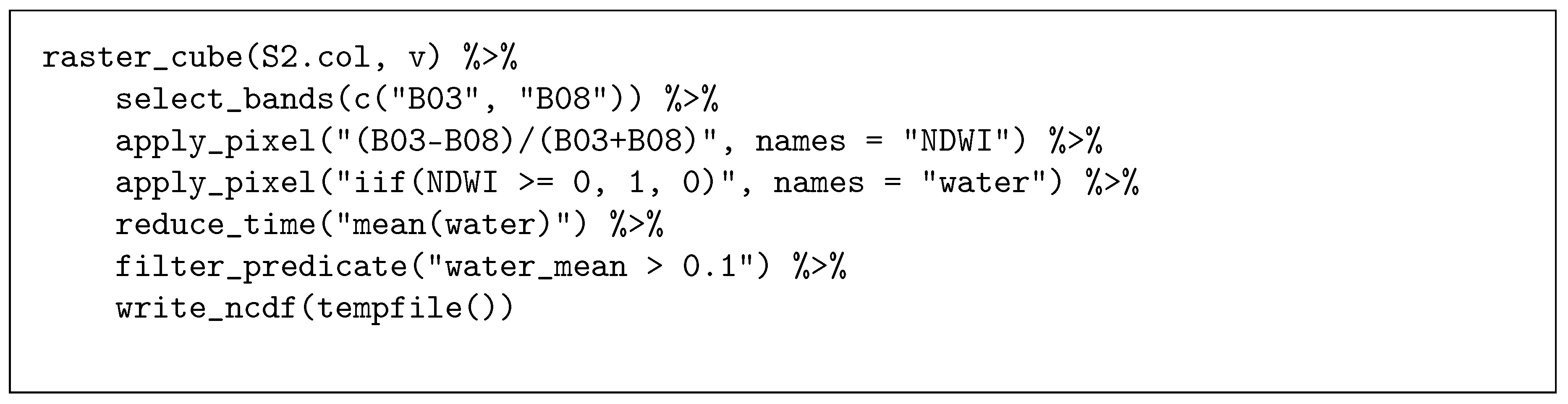
In a second study case, we applied a time series analysis on a collection of 102 Sentinel-2 images. The dataset covers the border region of Poland and Belarus, covering a total area of approximately 25,000 km. The images have been recorded between March and November 2018 and come from three different grid tiles and two different UTM zones. Images sum up to approximately 90 gigabytes and are stored as original compressed ZIP archives, downloaded from the Copernicus Open Access Hub [29]. Figure 8 shows the chain of data cube operations to detect permanent water bodies. We first compute the normalized difference water index (NDWI) based on green and near infrared reflectance, then simply classify all pixels with NDWI larger than or equal to zero as water (value 1), other pixels as no water (value 0), and then derive the mean over all pixel time series, representing the proportion of time instances where a pixel has been classified as water. In the last step, we set all pixels with value less than or equal 0.1 to NA and export the resulting image as a netCDF file. Figure 9 illustrates the study area and the results of the water detection on a low and high resolution in a map.
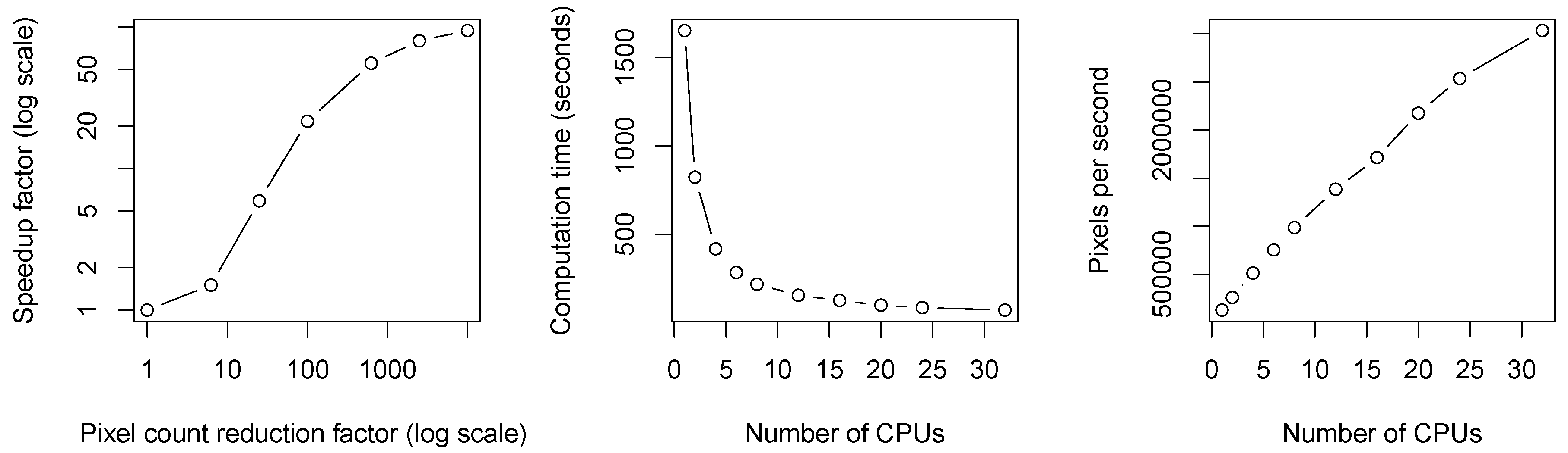
To evaluate how the implementation scales with the spatial resolution of the target data cube, we vary the spatial resolution in the data cube view and measure computation times for executing the code in Figure 8. At a fixed spatial resolution with pixels covering an area of 100 m × 100 m, we vary the number of used CPUs.
Figure 10 (left) shows how the speedup changed if the number of pixels was reduced by a certain factor. Reducing the number of pixels by a factor of 10,000, i.e., working with 1 km × 1 km pixel size compared to 10 m × 10 m, reduced the computation times by a factor of approximately 100. Although this may seem like a rather low effect, it means that we can process the whole dataset within less than a minute on low resolution as opposed to approximately one hour at full resolution. Computation times reduced consistently with an increasing number of CPUs (Figure 10). For example, we have been able to process 7.61 times more pixels per second when using eight threads compared to using a single thread.
4. Discussion
Today, data cubes are increasingly used as the basis for further analysis of large Earth observation image time series. For the creation of data cubes from image collections, resampling and/or aggregation in space and time is needed, in addition to image warping. As discussed below, the presented approach does this on-the-fly and interfaces existing open source software to process Earth observation data cubes.
4.1. Interactive Analyses of Large EO Datasets
The case studies have demonstrated that on-demand raster data cubes, where users define the shape of the target cube, allow the reduction of computation times and thus improve interactivity in analyses of large satellite image collections. This approach is similar to Google Earth Engine in that it only reads the pixels that are actually needed, as late as possible (lazy evaluation). However, the magnitude of reduction in computation times depends on particular data products. In the example of Sentinel-2 time series processing, gdalcubes makes use of provided image overviews or pyramids when working on a coarse resolution cube view. In contrast, MODIS products do not include such overviews and hence the full data must be read first, which reduces the gain in interactivity. In these cases, users may need to reduce the area and temporal range of interest to yield acceptable computation times. Under certain situations it might pay off to build overview images manually using the GDAL implementation before using gdalcubes. This also becomes important in cloud environments, where overviews may even reduce costs associated with data access or transfer.
There is currently quite some discussion about whether so-called analysis-ready data, which are essentially data cubes, should be processed for large scale imagery (e.g., [5] and CEOS-ARD6) in order to make these data usable for a larger community. As this creation is a very expensive operation, we argue in line with [3] that it is hard to create data cubes with parameters that satisfy every researcher, and that the on-the fly creation of data cubes retains maximum flexibility in this respect. More research on quantifying the loss of statistical accuracy or power due to resampling and working at lower-than-maximum resolutions is still needed.
4.2. Scalable and Distributed Processing in the Cloud
The examples shown here were executed on a local machine. Several days were needed to download the data, whereas the time for processing in the case study was much lower. While this is acceptable for medium-sized datasets, it becomes impossible for large scale, high resolution analyses. The rational trend is to move computations to cloud platforms where the data is already available. These include Amazon Web Services, the Google Cloud, and specialized EO data centers such as the Copernicus DIASes. Since the gdalcubes implementation uses GDAL to read imagery, it can directly access object storage from major cloud providers. Image collections then simply point to globally unique object storage identifiers and hence image collection indexes can be shared. Furthermore, though not yet available in the R package, the C++ implementation of gdalcubes comes with a prototypical server application, providing a simple REST-like API to process specific chunks of a cube. Running several of these gdalcubes worker instances in containerized cloud environments would allow process distribution over many compute instances.
An interesting open question is how the image collection index performs with much larger datasets. In the case studies with up to 34,000 images in a collection (global vegetation index data from MODIS for 5 years), we could not see any performance decreases so far. The image collection typically consumes a few kilobytes per image and images can be added incrementally. However, since the underlying table structure in the SQLite database only uses one-dimensional indexes on the spatial extent, acquisition time, and identifier of images, this might not scale well e.g., for the full Sentinel-2 archive. Implementations with more advanced indexes as in the S2 Geometry Library7 might be needed in these cases.
4.3. Interfaces to Other Software and Languages
The presented examples demonstrate how the gdalcubes library can be used in R. All data cube operations, the construction of data cubes from files, and the export as netCDF files are however implemented in C++. The R package is a thin software layer that makes the C++ library easily usable for R users. Since other languages such as Python or Julia also allow one to interface the C++ code, writing interfaces in these languages is feasible and relatively straightforward.
The data model to represent data cubes in memory is rather simple. A chunk is nothing more than a one-dimensional contiguous double precision C++ vector with additional attributes storing the dimensionality. As a result, it is also possible to interface and extend gdalcubes with linear algebra, image processing (e.g., Orfeo ToolBox [30]), or other external libraries including the NumPy C application programming interface [31].
The only other software systems we know of that can create regular data cubes from image collections are GRASS GIS [21], Open Data Cube [11], and the (non-open source) Google Earth Engine [3]. The open source library gdalcubes introduced here is a nice addition to these as it is relatively easy to integrate in scripting languages such as R, Julia, or Python, and can work in conjunction with software that can process data cubes such as GRASS GIS [32], R packages raster [16] and stars [17], and Python packages numpy [33] and xarray [13]. At the moment, a more user-friendly package to interface gdalcubes with the Python ecosystem is missing.
4.4. Limitations
The presented work focused on representing satellite imagery as raster data cubes and the implementation always uses a four-dimensional array with two spatial, one temporal, and one band dimension (see Definition 1). Hence, it is not directly applicable for higher dimensional data such as climate model output with vertical space or in cases where it is useful to represent time as two dimensions (e.g., year and day of year, or time of forecast and time to forecast). Furthermore, it currently represents raster data cubes only. Fortunately, the existing R package stars [17] implements generic multidimensional arrays, including support for rectilinear and curvilinear rasters and some first attempts to bring together functionalities from both packages are currently in progress.
The case studies demonstrated that the speed-up effect of on-demand data cubes on interactivity for lower resolution analyses strongly depends on particular datasets. One very important factor is whether the data comes with image pyramids/overviews, as well as the data format. In this regard, modern approaches such as the cloud-optimized GeoTIFF format with additional overviews seem very promising.
Similar to Google Earth Engine [3], the gdalcubes library is not well suited to problems that are hardly scalable and perform global analyses where results depend on distant pairs of pixels. There are also some parameters like the selection of chunk size, which are not easy to automatically optimize.
5. Conclusions
This paper proposes an approach to the on-demand creation of raster data cubes and presents an open source implementation in the gdalcubes library. It presents a generic solution to convert and combine irregular satellite imagery to regular raster data cubes, thereby supporting interactive incremental method development. This makes it easier for data users to exploit the potential of Earth observation data cubes such as combining data from several sensors and satellites. The organization of particular data products has a strong effect on speedups for computations on sub-sampled data. As the library has been written in C++, interfaces to scripting languages like Python and Julia could be developed easily; a gdalcubes R interface has been published on the Comprehensive R Archive Network (CRAN).
Author Contributions
Conceptualization, M.A.; Funding acquisition, M.A. and E.P.; Investigation, M.A.; Methodology, M.A.; Project administration, E.P.; Resources, M.A.; Software, M.A.; Supervision, E.P.; Visualization, M.A.; Writing—initial draft, M.A.; Writing—review & editing, E.P.
Funding
This research was funded by Deutsche Forschungsgemeinschaft under DFG project S3-GEP: Scalable Spatiotemporal Statistics for Global Environmental Phenomena, number 396611854.
Acknowledgments
The authors would like to thank two anonymous reviewers for their helpful comments and suggestions.
Conflicts of Interest
The authors declare no conflict of interest.
References
- Copernicus—The European Earth Observation Programme. Available online: https://ec.europa.eu/growth/sectors/space/copernicus_en (accessed on 14 June 2019).
- Lillesand, T.; Kiefer, R.W.; Chipman, J. Remote Sensing and Image Interpretation; John Wiley & Sons: New York, NY, USA, 2015. [Google Scholar]
- Gorelick, N.; Hancher, M.; Dixon, M.; Ilyushchenko, S.; Thau, D.; Moore, R. Google Earth Engine: Planetary-scale geospatial analysis for everyone. Remote Sens. Environ. 2017, 202, 18–27. [Google Scholar] [CrossRef]
- Lewis, A.; Oliver, S.; Lymburner, L.; Evans, B.; Wyborn, L.; Mueller, N.; Raevksi, G.; Hooke, J.; Woodcock, R.; Sixsmith, J.; et al. The Australian Geoscience Data Cube—Foundations and lessons learned. Remote Sens. Environ. 2017, 202, 276–292. [Google Scholar] [CrossRef]
- Giuliani, G.; Chatenoux, B.; Bono, A.D.; Rodila, D.; Richard, J.P.; Allenbach, K.; Dao, H.; Peduzzi, P. Building an Earth Observations Data Cube: Lessons learned from the Swiss Data Cube (SDC) on generating Analysis Ready Data (ARD). Big Earth Data 2017, 1, 100–117. [Google Scholar] [CrossRef]
- Lu, M.; Appel, M.; Pebesma, E. Multidimensional Arrays for Analysing Geoscientific Data. ISPRS Int. J. Geo-Inf. 2018, 7, 313. [Google Scholar] [CrossRef]
- Warmerdam, F. The geospatial data abstraction library. In Open Source Approaches in Spatial Data Handling; Springer: Berlin/Heidelberg, Germany, 2008; pp. 87–104. [Google Scholar]
- Baumann, P.; Dehmel, A.; Furtado, P.; Ritsch, R.; Widmann, N. The Multidimensional Database System RasDaMan. In Proceedings of the 1998 ACM SIGMOD International Conference on Management of Data, SIGMOD ’98, Seattle, WA, USA, 1–4 June 1998; ACM: New York, NY, USA, 1998; pp. 575–577. [Google Scholar]
- Stonebraker, M.; Brown, P.; Zhang, D.; Becla, J. SciDB: A Database Management System for Applications with Complex Analytics. Comput. Sci. Eng. 2013, 15, 54–62. [Google Scholar] [CrossRef]
- Appel, M.; Lahn, F.; Buytaert, W.; Pebesma, E. Open and scalable analytics of large Earth observation datasets: From scenes to multidimensional arrays using SciDB and GDAL. ISPRS J. Photogramm. Remote Sens. 2018, 138, 47–56. [Google Scholar] [CrossRef]
- Open Data Cube. Available online: https://www.opendatacube.org (accessed on 23 May 2019).
- Pangeo—A Community Platform for Big Data Geoscience. Available online: https://pangeo.io (accessed on 23 May 2019).
- Hoyer, S.; Hamman, J. xarray: ND labeled Arrays and Datasets in Python. J. Open Res. Softw. 2017, 5, 10. [Google Scholar] [CrossRef]
- Rocklin, M. Dask: Parallel computation with blocked algorithms and task scheduling. In Proceedings of the 14th Python in Science Conference, Austin, TX, USA, 6–12 July 2015; pp. 126–132. [Google Scholar]
- R Development Core Team. R: A Language and Environment for Statistical Computing; R Foundation for Statistical Computing: Vienna, Austria, 2008; ISBN 3-900051-07-0. [Google Scholar]
- Hijmans, R.J. raster: Geographic Data Analysis and Modeling, R Package Version 2.9-5; 2019. Available online: https://CRAN.R-project.org/package=raster (accessed on 27 June 2019).
- Pebesma, E. stars: Spatiotemporal Arrays, Raster and Vector Data Cubes, R Package Version 0.3-1; 2019. Available online: https://CRAN.R-project.org/package=stars (accessed on 27 June 2019).
- Baumann, P.; Rossi, A.P.; Bell, B.; Clements, O.; Evans, B.; Hoenig, H.; Hogan, P.; Kakaletris, G.; Koltsida, P.; Mantovani, S.; et al. Fostering Cross-Disciplinary Earth Science Through Datacube Analytics. In Earth Observation Open Science and Innovation; Mathieu, P.P., Aubrecht, C., Eds.; Springer International Publishing: Cham, Switzerland, 2018; pp. 91–119. [Google Scholar] [Green Version]
- Nativi, S.; Mazzetti, P.; Craglia, M. A view-based model of data-cube to support big earth data systems interoperability. Big Earth Data 2017, 1, 75–99. [Google Scholar] [CrossRef] [Green Version]
- Strobl, P.; Baumann, P.; Lewis, A.; Szantoi, Z.; Killough, B.; Purss, M.; Craglia, M.; Nativi, S.; Held, A.; Dhu, T. The Six Faces of The Datacube. In Proceedings of the 2017 Conference on Big Data from Space (BIDS’ 2017), Toulouse, France, 28–30 November 2017; pp. 28–30. [Google Scholar]
- Gebbert, S.; Leppelt, T.; Pebesma, E. A Topology Based Spatio-Temporal Map Algebra for Big Data Analysis. Data 2019, 4, 86. [Google Scholar] [CrossRef]
- Rew, R.; Davis, G. NetCDF: An interface for scientific data access. IEEE Comput. Graph. Appl. 1990, 10, 76–82. [Google Scholar] [CrossRef]
- SQLite. Available online: https://www.sqlite.org (accessed on 24 May 2019).
- Stenberg, D.; Fandrich, D.; Tse, Y. libcurl: The Multiprotocol File Transfer Library. Available online: http://curl.haxx.se/libcurl (accessed on 24 May 2019).
- Tinyexpr. Available online: https://github.com/codeplea/tinyexpr (accessed on 24 May 2019).
- Date. Available online: https://howardhinnant.github.io/date/date.html (accessed on 24 May 2019).
- Tiny-process-library. Available online: https://gitlab.com/eidheim/tiny-process-library (accessed on 24 May 2019).
- JSON for Modern C++. Available online: https://github.com/nlohmann/json (accessed on 24 May 2019).
- Copernicus Open Access Hub. Available online: https://scihub.copernicus.eu (accessed on 24 May 2019).
- Inglada, J.; Christophe, E. The Orfeo Toolbox remote sensing image processing software. In Proceedings of the 2009 IEEE International Geoscience and Remote Sensing Symposium, Cape Town, South Africa, 12–17 July 2009; Volume 4, pp. 76–82. [Google Scholar]
- NumPy C-API. Available online: https://docs.scipy.org/doc/numpy/reference/c-api.html (accessed on 14 June 2019).
- Neteler, M.; Bowman, M.; Landa, M.; Metz, M. GRASS GIS: A multi-purpose Open Source GIS. Environ. Model. Softw. 2012, 31, 124–130. [Google Scholar] [CrossRef]
- Walt, S.V.D.; Colbert, S.C.; Varoquaux, G. The NumPy Array: A Structure for Efficient Numerical Computation. Comput. Sci. Eng. 2011, 13, 22–30. [Google Scholar] [CrossRef] [Green Version]
| 1 | |
| 2 | |
| 3 | |
| 4 | |
| 5 | |
| 6 | |
| 7 |
Figure 1.
Data structure for image collections in gdalcubes. Geospatial Data Abstraction Library (GDAL) datasets refer to actual image data, which can be local or remote files, objects in cloud storage, sub-datasets in a more complex file format, or any other resources that GDAL can read.
Figure 1.
Data structure for image collections in gdalcubes. Geospatial Data Abstraction Library (GDAL) datasets refer to actual image data, which can be local or remote files, objects in cloud storage, sub-datasets in a more complex file format, or any other resources that GDAL can read.

Figure 2.
Typical analysis workflow for users of the R package gdalcubes.

Figure 3.
Example R script to derive a mosaic preview of Sentinel-2 images by calculating the median of visible bands over pixel time series.
Figure 3.
Example R script to derive a mosaic preview of Sentinel-2 images by calculating the median of visible bands over pixel time series.

Figure 4.
Output of R script in Figure 3, plotting median reflectances of visible Sentinel-2 bands over time.
Figure 4.
Output of R script in Figure 3, plotting median reflectances of visible Sentinel-2 bands over time.

Figure 5.
Screenshot of using Google Earth Engine [3] to apply a median RGB reduction of Sentinel-2 images for the same study area and time as used in Figure 3 and Figure 4. Background imagery and map data © 2019 GeoBasis-DE/BKG (© 2019), Google.

Figure 6.
R script to combine data cubes from three different data products. The construction of the image collection is omitted here.
Figure 6.
R script to combine data cubes from three different data products. The construction of the image collection is omitted here.

Figure 7.
Temporal subset of the combined data cube with NDVI measurements (left), average daytime land surface temperature (K) during the last 30 days (center), and average daily precipitation (mm) during the last 30 days (right).
Figure 7.
Temporal subset of the combined data cube with NDVI measurements (left), average daytime land surface temperature (K) during the last 30 days (center), and average daily precipitation (mm) during the last 30 days (right).

Figure 8.
R script to detect permanent water bodies from a Sentinel-2 data cube.

Figure 9.
Result map from water detection in the second study case. The right part illustrates the results at a high spatial resolution.
Figure 9.
Result map from water detection in the second study case. The right part illustrates the results at a high spatial resolution.

Figure 10.
Computational results for the second study case. The left plot shows the achieved speedup factors depending on the reduction of pixels in the target data cube. For example, reducing the number of pixels by a factor of 100 resulted in a speedup of around 20, compared to computation times with a 10 m by 10 m spatial resolution. The center and right plots show computation times and pixel throughput respectively as a function of the number of used CPUs.


Table 1.
Implemented data cube operations in the current version of the gdalcubes library.
| Operator | Description |
|---|---|
| raster_cube | Create a raster data cube from an image collection and a data cube view |
| reduce_time | Apply a reducer function independently over all pixel time series |
| reduce_space | Apply a reducer function independently over all spatial slices |
| apply_pixel | Apply an arithmetic expression on band values over all pixels |
| filter_pixel | Filter pixels with a logical predicate on one or more band values |
| join_bands | Stack the bands of two identically shaped cubes in a single cube |
| window_time | Apply a reducer function or kernel filter over moving windows for all pixel time series |
| write_ncdf | Export a data cube as a netCDF file |
| chunk_apply | Apply a user-defined function over chunks of a data cube |
Table 2.
Summary of the data products as used in the first study case. Definitions: GPM, Global Precipitation Measurement mission; NDVI, normalized difference vegetation index; liquid_accum, liquid daily accumulated precipitation; LST_DAY, daytime land surface temperature; SRS, spatial reference system; MODIS, Moderate Resolution Imaging Spectroradiometer.
| MOD13A2 | GPM | MOD11A1 | |
|---|---|---|---|
| Selected Variables | NDVI | liquid_accum | LST_DAY |
| Spatial Resolution | 1 km × 1 km | 0.1 × 0.1 | 1 km × 1 km |
| Area of Interest | global (land only) | global (60 N–60 S full) | Europe (land only) |
| Temporal Resolution | 16 days | daily | daily |
| Time Range | 2014-01-01–2019-01-01 | 2014-01-01–2019-01-01 | 2014-01-01–2019-01-01 |
| File Format | HDF4 | GeoTIFF (zip compressed) | HDF4 |
| SRS | MODIS sinusoidal | Lat/Lon grid | MODIS sinusoidal |
© 2019 by the authors. Licensee MDPI, Basel, Switzerland. This article is an open access article distributed under the terms and conditions of the Creative Commons Attribution (CC BY) license (http://creativecommons.org/licenses/by/4.0/).
Share and Cite
MDPI and ACS Style
Appel, M.; Pebesma, E. On-Demand Processing of Data Cubes from Satellite Image Collections with the gdalcubes Library. Data 2019, 4, 92. https://0-doi-org.brum.beds.ac.uk/10.3390/data4030092
AMA Style
Appel M, Pebesma E. On-Demand Processing of Data Cubes from Satellite Image Collections with the gdalcubes Library. Data. 2019; 4(3):92. https://0-doi-org.brum.beds.ac.uk/10.3390/data4030092
Chicago/Turabian StyleAppel, Marius, and Edzer Pebesma. 2019. "On-Demand Processing of Data Cubes from Satellite Image Collections with the gdalcubes Library" Data 4, no. 3: 92. https://0-doi-org.brum.beds.ac.uk/10.3390/data4030092