Classification of Soils into Hydrologic Groups Using Machine Learning

Department of Electrical and Computer Engineering, Seattle University, Seattle, WA 98122, USA
*
Author to whom correspondence should be addressed.
Data 2020, 5(1), 2; https://0-doi-org.brum.beds.ac.uk/10.3390/data5010002
Submission received: 1 October 2019
/
Revised: 15 December 2019
/
Accepted: 15 December 2019
/
Published: 19 December 2019
(This article belongs to the Special Issue Overcoming Data Scarcity in Earth Science)
Abstract
:Hydrologic soil groups play an important role in the determination of surface runoff, which, in turn, is crucial for soil and water conservation efforts. Traditionally, placement of soil into appropriate hydrologic groups is based on the judgement of soil scientists, primarily relying on their interpretation of guidelines published by regional or national agencies. As a result, large-scale mapping of hydrologic soil groups results in widespread inconsistencies and inaccuracies. This paper presents an application of machine learning for classification of soil into hydrologic groups. Based on features such as percentages of sand, silt and clay, and the value of saturated hydraulic conductivity, machine learning models were trained to classify soil into four hydrologic groups. The results of the classification obtained using algorithms such as k-Nearest Neighbors, Support Vector Machine with Gaussian Kernel, Decision Trees, Classification Bagged Ensembles and TreeBagger (Random Forest) were compared to those obtained using estimation based on soil texture. The performance of these models was compared and evaluated using per-class metrics and micro- and macro-averages. Overall, performance metrics related to kNN, Decision Tree and TreeBagger exceeded those for SVM-Gaussian Kernel and Classification Bagged Ensemble. Among the four hydrologic groups, it was noticed that group B had the highest rate of false positives.
1. Introduction
Soils play a crucial role in the global hydrologic cycle by governing the rates of infiltration and transmission of rainfall, and surface runoff, i.e., precipitation that does not infiltrate into the soil and runs across the land surface into water bodies, such as streams, rivers and lakes. Runoff occurs when rainfall exceeds the infiltration capacity of soils, and it is based on the physical nature of soils, land cover, hillslope, vegetation and storm properties such as rainfall duration, amount and intensity. The rainfall-runoff process serves as a catalyst for the transport of sediments and contaminants, such as fertilizers, pesticides, chemicals and organic matter, negatively impacting the morphology and biodiversity of receiving water bodies [1,2]. Flooding and erosion caused by uncontrolled runoff, particularly downstream, results in damage to agricultural lands and manmade structures [1]. Hence, modeling surface runoff is an essential part of soil and water conservation efforts, including but not limited to, forecasting floods and soil erosion and monitoring water and soil quality.
The U.S. Department of Agriculture’s (USDA) agency for Natural Resources Conservation Service (NRCS), formerly known as the Soil Conservation Service (SCS), developed a parameter called Curve Number (CN) to estimate the amount of surface runoff. Furthermore, soils are classified into Hydrologic Soil Groups (HSGs) based on surface conditions (infiltration rate) and soil profiles (transmission rate). Combinations of HSGs and land use and treatment classes form hydrologic soil-cover complexes, each of which is assigned a CN [3]. A higher CN indicates a higher runoff potential. Consequently, accurate classification of HSGs is critical for the calculation of CNs that provide a meaningful prediction of runoff.
In the United States, more than 19,000 soil series have been identified and aggregated into map unit components with similar physical and runoff characteristics, and assigned to one of four HSGs: A, B, C or D. The original assignments were based on measured rainfall, runoff and infiltrometer data [4]. Since then, assignments have been based on the judgement of soil scientists, primarily relying on their interpretation of criteria published in the National Engineering Handbook (NEH) Part 630, Hydrology [5]. As with any subjective interpretation, the placement of soils into appropriate hydrologic groups have been non-uniform and inconsistent over time and across geographical locations. Soils with similar runoff characteristics were placed in the same hydrologic group, under the assumption that soils found within a climatic region with similar depth, permeability and texture will have similar runoff responses. Conventional soil mapping techniques extrapolate these classifications and geo-reference them with GPS (Global Positioning Systems) and digital elevation models visualized in a GIS (Geographic Information Systems) [6,7]. However, in addition to the inconsistent classification of soil profiles, the varying definition of mapping units introduces a certain degree of subjectivity. Over the past two decades, Pedology research has witnessed an evolution from traditional soil mapping techniques to methods for ‘the creation and population of spatial soil information systems by numerical models inferring the spatial and temporal variations or soil types and soil properties from soil observation and knowledge and from related environmental variables’ [8], also known as Digital Soil Mapping (DSM) [9,10,11].
Considering the advances in modern computing and the vastly expanding soil databases, NRCS and the Agricultural Research Service (ARS) formed a joint working group in 1990 to address shortcomings attributed to guidelines stated in NEH reference documents [12]. Two among the several goals identified by the group were to standardize the procedure for the calculation of CNs from rainfall-runoff data and to reconsider the HSG classifications. A fuzzy model that was developed using the National Soil Information System (NASIS) soil interpretation subsystem was applied to 1828 unique soils using data from Kansas, South Dakota, Missouri, Iowa, Wyoming and Colorado. Correlation between the soil’s assigned and modeled HSG was analyzed, and the overall HSG frequency coincidence exceeded 54 percent [13]. It was observed that the correlation frequencies for soils from groups A and D were higher than those for groups B and C. These correlation inconsistencies were attributed to: (1) boundary conditions that occur when soils exhibit properties that do not fit entirely into a single hydrologic group. The effects of this are more profound for groups B and C considering that they are each bounded by two groups (2) fuzzy modeling of the subjective HSG criteria. To address the inconsistencies due to boundary conditions, an improved method that developed an automated system based on detailed soil attribute data was proposed by Li, R et al. [14]. This work aimed to mitigate the aggregation effect of HSGs on soil information, and eventually the CNs, due to the assignment of similar soils into different HSGs (exaggerating small differences between them) or different soils to the same HSG (omitting differences between them). Furthermore, this work successfully identified improper placement of HSGs. However, this work used a significantly smaller sample size of 67 soil types in the Lake Fork watershed in Texas.
Machine learning, a branch of Artificial Intelligence, is an inherently interdisciplinary field that is built on concepts such as probability and statistics, information theory, game theory and optimization, among many others. In 1959, Arthur Samuel, one of the pioneers of machine learning, defined machine learning as a “field of study that gives computers the ability to learn without being explicitly programmed” [15]. A more recent and widely accepted definition can be attributed to Tom Mitchell: “A computer program is said to learn from experience E with respect to some class of tasks T and performance measure P, if its performance at tasks in T, as measured by P, improves with experience E” [16]. Based on the approach used, type of input and output data, and nature of the problem being addressed, machine learning techniques can be classified into four main categories: (1) supervised learning; (2) unsupervised learning; (3) semi-supervised learning; and (4) reinforcement learning.
In supervised learning, the goal is to infer a function or mapping from training data that is labeled. The training data consist of an input vector X and an output vector Y that is labeled based on available prior experience. Regression and classification are two categories of algorithms that are based on supervised learning. Unsupervised learning, on the other hand, deals with unlabeled data, with the goal of finding a hidden structure or pattern in this data. Clustering is one of the most widely used unsupervised learning methods. In semi-supervised learning, a combination of labeled and unlabeled data is used to generate an appropriate model for the classification of data. The reinforcement learning method uses observations gathered from the interaction with the environment to make a sequence of decisions that would maximize the reward or minimize the risk. Q-learning is an example of a reinforcement learning algorithm.
The application of machine learning techniques in soil sciences ranges from the prediction of soil classes using DSM [17,18] to the classification of sub-soil layers using segmentation and feature extraction [19]. The predictive ability of machine learning models has been leveraged for agricultural planning and mass crop yield, the prediction of natural hazards, including, but not limited to, landslides, floods, drought and forest fires and monitoring the effects of climate change on the physical and chemical properties of soil [20,21]. Based on high spatial resolution satellite data, terrain/climatic data, and laboratory soil samples, the spatial distribution of six soil properties including sand, silt, and clay were mapped in an agricultural watershed in West Africa [22]. Of the four statistical prediction models tested and compared, i.e., Multiple Linear Regression (MLR), Random Forest Regression (RFR), Support Vector Machine (SVM) and Stochastic Gradient Boosting (SGB), machine learning algorithms performed generally better than MLR for the prediction of soil properties at unsampled locations. In a similar study for a steep-slope watershed in southeastern Brazil [23], the performance of three algorithms: Multinomial Logistic Regression (MLR), C5-decision tree (C5-DT) and Random Forest (RF) was evaluated and compared based on performance metrices of overall accuracy, standard error, and kappa index. It was observed that the RF model consistently outperformed the other models, while the MLR model had the lowest overall accuracy and kappa index. In the context of DSM applications, complex models such as RF are found to be better classifiers than generalized linear models such as MLR. While machine learning offers the added advantage of identifying trends and patterns with continuous improvement over time, these models are only as good as the quality of the data collected. An unbiased and inclusive dataset, along with the right choice of model, parameters, cross-validation method, and performance metrices is necessary to achieve meaningful results.
In this work, we investigated the application of four machine learning methods: kNN, SVM-Gaussian Kernel, Decision Trees and Ensemble Learning towards the classification of soil into hydrologic groups. The results of these algorithms are compared to those obtained using estimation based on soil texture.
2. Background
Soils are composed of mineral solids derived from geologic weathering, organic matter solids consisting of plant or animal residue in various stages of decomposition, and air and water that fill the pore space when soil is dry and wet, respectively. The mineral solid fraction of soil is composed of sand, silt and clay, relative percentages of which determine the soil texture in accordance with the USDA system of particle-size classification. Sand, being the larger of the three, feels gritty, and ranges in size from 0.05 to 2.00 mm. Sandy soils have poor water-holding capacity that can result in leaching loss of nutrients. Silt, being moderate in size, has a smooth or floury texture, and ranges from 0.002 to 0.05 mm. Clay, being the smallest of the three, feels sticky, and is made up of particles smaller than 0.002 mm in diameter. In general, the higher the percentage of silt and clay particles in soil, the higher is its water-holding capacity. Particles larger than 2.0 mm are referred to as rock fragments and are not considered in determining soil texture, although they can influence both soil structure and soil–water relationships. The ease with which pores in a saturated soil transmit water is known as saturated hydraulic conductivity (Ksat), and it is expressed in terms of micrometers per second (or inches per hour). Pedotransfer functions (PTFs) are commonly used to estimate Ksat in terms of readily available soil properties such as particle size distribution, bulk density, and organic matter content [24,25]. Machine Learning-based PTFs have been developed to understand the relationship between soil hydraulic properties and soil physical variables [26].
Hydrologic Soil Groups
Soils are classified into HSGs based on the minimum rate of infiltration obtained for bare soil after prolonged wetting [5]. The four hydrologic soil groups (HSGs) are described as follows:
- Group A—Soils in this group are characterized by low runoff potential and high infiltration rates when thoroughly wet. They typically have less than 10 percent clay and more than 90 percent sand or gravel. The saturated hydraulic conductivity of all soil layers exceeds 40.0 micrometers per second.
- Group B—Soils in this group have moderately low runoff potential and moderate infiltration rates when thoroughly wet. They typically have between 10 and 20 percent clay and 50 to 90 percent sand. The saturated hydraulic conductivity ranges from 10.0 to 40.0 micrometers per second.
- Group C—Soils in this group have moderately high runoff potential and low infiltration rates when thoroughly wet. They typically have between 20 and 40 percent clay and less than 50 percent sand. The saturated hydraulic conductivity ranges from 1.0 to 10.0 micrometers per second.
- Group D—Soils in this group are characterized by high runoff potential and very low infiltration rates when thoroughly wet. They typically have greater than 40 percent clay and less than 50 percent sand. The saturated hydraulic conductivity is less than or equal to 1.0 micrometers per second.
- Dual hydrologic soil groups—Certain wet soils are placed in group D based solely on the presence of a high water table. Once adequately drained, they are assigned to dual hydrologic soil groups (A/D, B/D and C/D) based on their saturated hydraulic conductivity. The first letter applies to the drained condition and the second to the undrained condition.
3. Methods
3.1. Soil Survey Data
The dataset used for this work was obtained from USDA’s NRCS Web Soil Survey (WSS), the largest public-facing natural resource database in the world [27]. The Soil Survey Geographic Database (SSURGO) developed by the National Cooperative Soil Survey was used to identify Areas of Interests (AOI) in the State of Washington the Idaho Panhandle National Forest. Tabular data corresponding to Physical Soil Properties and Revised Universal Soil Loss Equation, Version 2 (RUSLE2) related attributes for various AOIs were retrieved from the Microsoft Access database and compiled into Microsoft Excel spreadsheets. Features of interest include the map symbol and soil name, its corresponding hydrologic group, percentages of sand, silt and clay, depth in inches and Ksat in micrometers per second. The initial dataset comprised of 4468 unique soil types.
As with most survey-based datasets, there were incomplete or missing data, inconsistencies in formatting and undesired data entries. The compiled dataset was preprocessed to remove samples corresponding to: missing data points, dual hydrologic groups (A/D, B/D and C/D), and soil layers beyond a water impermeable depth range of 20 to 40 inches. This reduced the dataset to 2107 unique soil types. MATLAB® programming environment was used for all data preparation and processing.
3.2. Estimation Based on Soil Texture
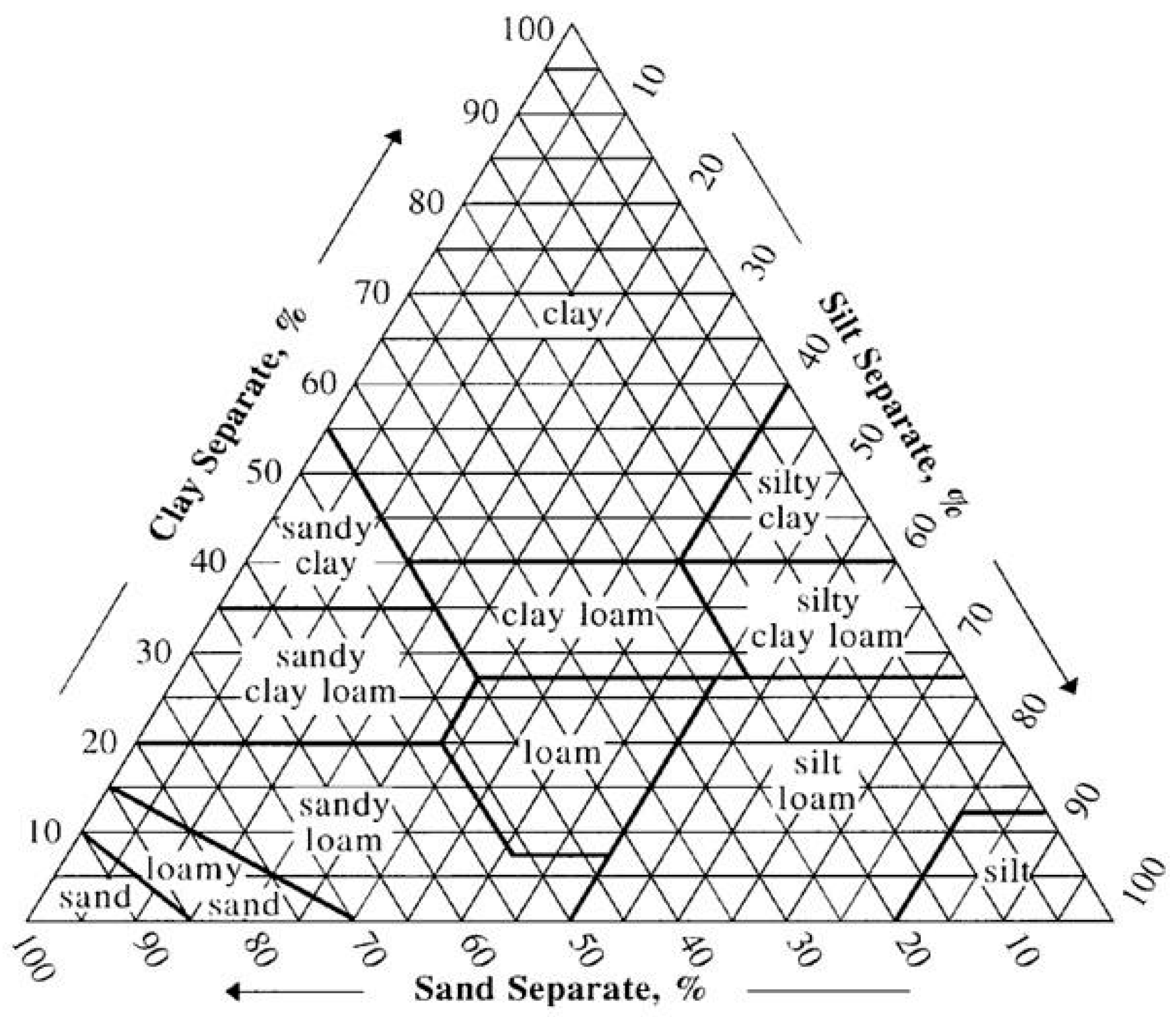
Based on the percentages of sand, silt, and clay, soils can be grouped into one of the four major textural classes: (1) sands; (2) silts; (3) loams; and (4) clays. The soil textural triangle shown in Figure 1 illustrates twelve textural classes as defined by the USDA [28]: sand, loamy sand, sandy loam, loam, silt loam, silt, sandy clay loam, clay loam, silty clay loam, sandy clay, silty clay, and clay. These classifications are typically named after the primary constituent particle size, e.g., “sand”, or a combination of the most abundant particles sizes, e.g., “sandy clay”. One side of the triangle represents percent sand, the second side represents percent clay, and the third side represents percent silt. Given the percentages of sand, silt and clay in the soil sample, the corresponding textural class can be read from the triangle. Alternately, the NRCS soil texture calculator [28] can be used to determine textural class based on specific relationships between sand, silt and clay percentages as shown in Table 1. In this work, the method used to assign HSGs based on soil texture was adopted from Hong and Adler (2008) [29], which was modified from the USDA handbook [30] and National Engineering Handbook Section 4 [5]. MATLAB® was used to assign HSGs based on soil texture calculations.
3.3. Machine Learning Algorithms
A common problem encountered in machine learning and data science is that of overfitting, where the model does not generalize well from training data to unseen data. Cross validation techniques are generally used to assess the generalization ability of a predictive model, thus avoiding the problem of overfitting. In this work, a Monte Carlo Cross-Validation (MCCV) method [31] was used by randomly splitting the dataset into equal-sized training and test subsets, training the model, predicting classification and repeating the process 100 times. The overall prediction accuracy (or other performance metrics) is the average over all iterations.
A machine learning algorithm can be classified as either parametric or non-parametric. Parametric methods assume a finite and fixed set of parameters, independent of the number of training examples. In non-parametric methods, also called instance-based or memory-based learning, the number of parameters is determined in part by the data, i.e., the number of parameters grows with the size of the training set. Due to the availability of a large dataset with labeled data, in this work, we considered four non-parametric supervised learning algorithms: (1) kNN (2) SVM Gaussian Kernel (3) Decision Trees (4) Random Forest. A qualitative introduction to these algorithms is presented in the following subsections.
3.3.1. k-Nearest Neighbors (kNN) Algorithm
kNN algorithm, an instance-based method of learning, is based on the principle that instances within a dataset will generally exist in close proximity to other instances that have similar properties. If the instances are tagged with a classification label, then the value of the label of an unclassified instance can be predicted based on the labels of its nearest neighbors.
The Statistics and Machine Learning Toolbox from MATLAB® was used to create a Classification kNN model using function ‘fitcknn’, followed by the function ‘predict’ to predict classification for test data.
- knn_model = fitcknn (features, labels, ‘NumNeighbors’, k)
- predict_HSG = predict (knn_model, features_test)
where features is a numeric matrix that contains percent sand, percent silt, percent clay and Ksat; label is a cell array of character vectors that contain the corresponding HSGs; and k represents the number of neighbors.
3.3.2. Support Vector Machines (SVMs) with Gaussian Kernel
Support Vector Machines are non-parametric, supervised learning models that are motivated by a geometric idea of what makes a classifier “good” [32]. For linearly separable data points, the objective of the SVM algorithm is to find an optimal hyperplane (or a decision boundary) in an N-dimensional space (where N is the number of features) that distinctly classifies data points. Support vectors are the data points that lie closest to the hyperplane. The SVM algorithm aims to maximize the margin around the separating hyperplane, essentially making it a constrained optimization problem.
For data points that are not linearly separable, which is true of most real-world data, the features can be mapped into a higher-dimensional space in such a way that the classes become more easily separated than in the original feature space. A technique commonly referred to as the ‘kernel trick’, uses a kernel function that defines the inner product of the mapping functions in the transformed space. One of the most popular kernels are the Radial Basis Functions (RBFs), of which, the Gaussian kernel is a special case.
The Statistics and Machine Learning Toolbox from MATLAB® was used to create a template for SVM binary classification based on a Gaussian kernel function using function ‘templateSVM’, followed by the function ‘fitcecoc’ that trains an Error-Correcting Output Codes (ECOC) model based on the features and labels provided. t is specified as a binary learner for an ECOC multiclass model. Finally, the function ‘predict’ is used to predict classification for test data.
- t = templateSVM (‘KernelFunction’, ‘gaussian’)
- SVM_gaussian_model = fitcecoc (features, labels, ‘Learners’, t);
- predict_HSG = predict (SVM_gaussian_model, features_test)
3.3.3. Decision Trees
Decision Trees are hierarchical models for supervised learning in which the learned function is represented by a decision tree [16,33]. The model classifies instances by querying them down the tree from the root to a leaf node, where each node represents a test over an attribute, each branch denotes its outcomes and each leaf node represents one class. Based on the measure used to select input variables and the type of splits at each node, decision trees can be implemented using statistical algorithms such as CART (Classification And Regression Tree), ID3 (Iterative Dichotomiser 3) and C4.5 (successor of ID3), among many others.
The Statistics and Machine Learning Toolbox from MATLAB® was used to grow a fitted binary classification decision tree based on the features and labels using function ‘fitctree’, followed by the function ‘predict’ to predict classification for test data. Function ‘fitctree’ uses the standard CART algorithm to grow decision trees.
- decisiontree_model = fitctree (features, labels);
- predict_HSG = predict (decisiontree_model, features_test)
3.3.4. Ensemble Learning
While decision trees are a popular choice for predictive modeling due to their inherent simplicity and intuitiveness, they are often characterized by high variance. Consequently, decision trees can be unstable because small variations in the data might result in a completely different tree and hence, a different prediction. Ensemble learning methods that combine and average over multiple decision trees have been used to improve predictive performance [32]. Bagging (or bootstrap aggregation) is a technique that is used to generate new datasets with approximately the same (unknown) sampling distribution as any given dataset. Random forests, an extension of the bagging method, also selects a random subset of features. In other words, random forests can be considered as a combination of ‘bootstrapping’ and ‘feature bagging’.
The Statistics and Machine Learning Toolbox from MATLAB® was used to grow an ensemble of learners for classification using function ‘fitcensemble’’, followed by the function ‘predict’ to predict classification for test data.
- ensemble_model = fitcensemble (features, labels);
- predict_HSG = predict (ensemble_model, features_test);
The function ‘TreeBagger’ bags an ensemble of decision trees for classification using the Random Forest algorithm, followed by the function ‘predict’ to predict classification for test data. Decision trees in the ensemble are grown using bootstrap samples of the data, with a random subset of features to use at each decision split.
- treebagger_model = TreeBagger (50, features, labels, ‘OOBPrediction’, ‘On’, ‘OOBPredictorImportance’, ‘On’);
- predicted_HSG = predict (treebagger_model, features_test);
‘OOBPrediction’ and ‘OOBPredictorImportance’ are set to ‘on’ to store information on what observations are out of bag for each tree and to store out-of-bag estimates of feature importance in the ensemble, respectively.
4. Performance Metrics
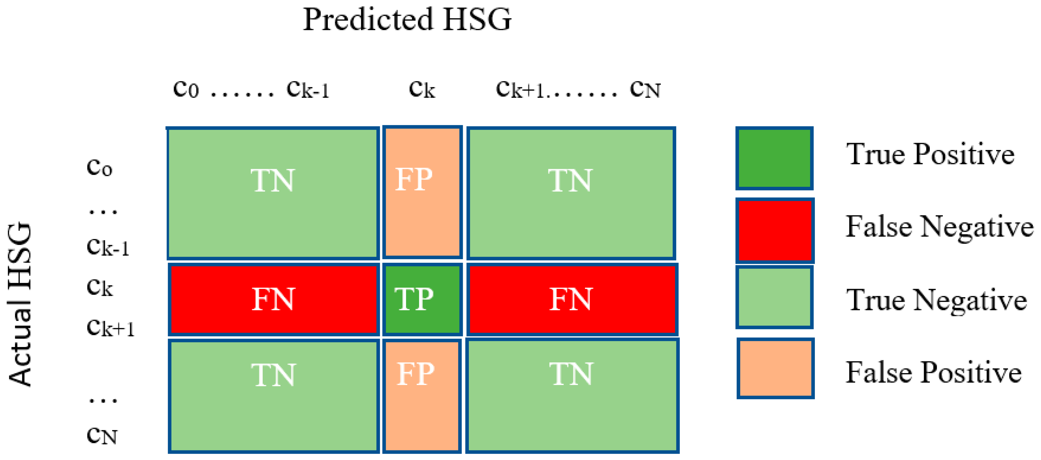
A Confusion matrix is commonly used to visualize the performance of a classification algorithm. Figure 2 illustrates the confusion matrix for a multi-class model with N classes [34]. Observations on correct and incorrect classifications are collected into the confusion matrix , where represents the frequency of class i being identified as class j. In general, the confusion matrix provides four types of classification results with respect to one classification target k:
- True Positive (TP)—correct prediction of the positive class ()
- True Negative (TN)—correct prediction of the negative class ()
- False Positive (FP)—incorrect prediction of the positive class ()
- False Negative (FN)—incorrect prediction of the negative class ()
Several performance metrics can be derived from these four outcomes. The ones of interest to us are listed below, for per-class classifications:
- Accuracy: This metric simply measures how often the classifier makes a correct prediction.
- Recall (Sensitivity or True Positive Rate): This metric denotes the classifier’s ability to predict a correct class
- Precision: This metric represents the classifier’s certainty of correctly predicting a given class
- False Positive Rate (FPR): This metric represents the number of incorrect positive predictions out of the total true negatives
- True Negative Rate (TNR or Specificity): This metric represents the number of correct negative predictions out of the total true negatives
- F1-Score: This metric is a harmonic mean of precision and recall. Although the F1-score is not as intuitive as accuracy, it is useful in measuring how precise and robust the classifier is.
- Matthews Correlation Coefficient (MCC): For binary classification, MCC summarizes into a single value the confusion matrix. This is easily generalizable to multi-class problems as well.
- Cohen’s Kappa (κ): This metric compares an Observed Accuracy with an Expected Accuracy (random chance)where represents the accuracy and represents a factor that is based on normalized marginal probabilities.
For multi-class classification problems, averaging per-class metric results can provide an overall measure of the model’s performance. There are two widely used averaging techniques: macro-averaging and micro-averaging.
- Macro-average: Macro-averaging reduces the multi-class predictions down to multiple sets of binary predictions. The desired metric for each of the binary cases are calculated and then averaged resulting in the macro-average for the metric over all classes. For example, the macro-average for Recall is calculated as shown below:
- Micro-average: Micro-averaging uses individual true positives, true negatives, false positives and false negatives from all classes to calculate the micro-average. For example, the micro-average for Recall is calculated as shown below:
Macro-averaging assigns equal weight to each class, whereas micro-averaging assigns equal weight to each observation. Micro-averages provide a measure of effectiveness on classes with large observations, whereas macro-averages provide a measure of effectiveness on classes with small observations.
5. Results and Discussions
Following data preparation and pre-processing in MATLAB®, soil data samples were classified into one of the four hydrologic groups using soil texture calculations, followed by classifications using the following algorithms: (a) k-Nearest Neighbor (kNN), (b) SVM Gaussian Kernel, (c) Decision Tree, (d) Classification Bagged Ensemble, and (e) TreeBagger. A Monte Carlo Cross-Validation (MCCV) method was used to avoid the problem of overfitting [31]. A measure of overall accuracy was first computed to compare all five algorithms with the soil texture-based classification. Table 2 shows that overall accuracy for the latter is significantly lower than those for the machine learning-based classification algorithms. In fact, none of the HSG C occurrences were correctly classified using soil texture calculations. The TreeBagger (Random Forest) algorithm has the highest overall accuracy of 84.70 percent, closely followed by the Decision Tree and kNN algorithms with 83.12 percent and 80.66 percent, respectively. Although applied for an entirely different dataset, the fuzzy system hydrologic grouping model [13] results in an overall correlation frequency of 60.5 percent for HSGs A, B, C and D, with higher correlation between assigned and modeled results for HSGs A and D.
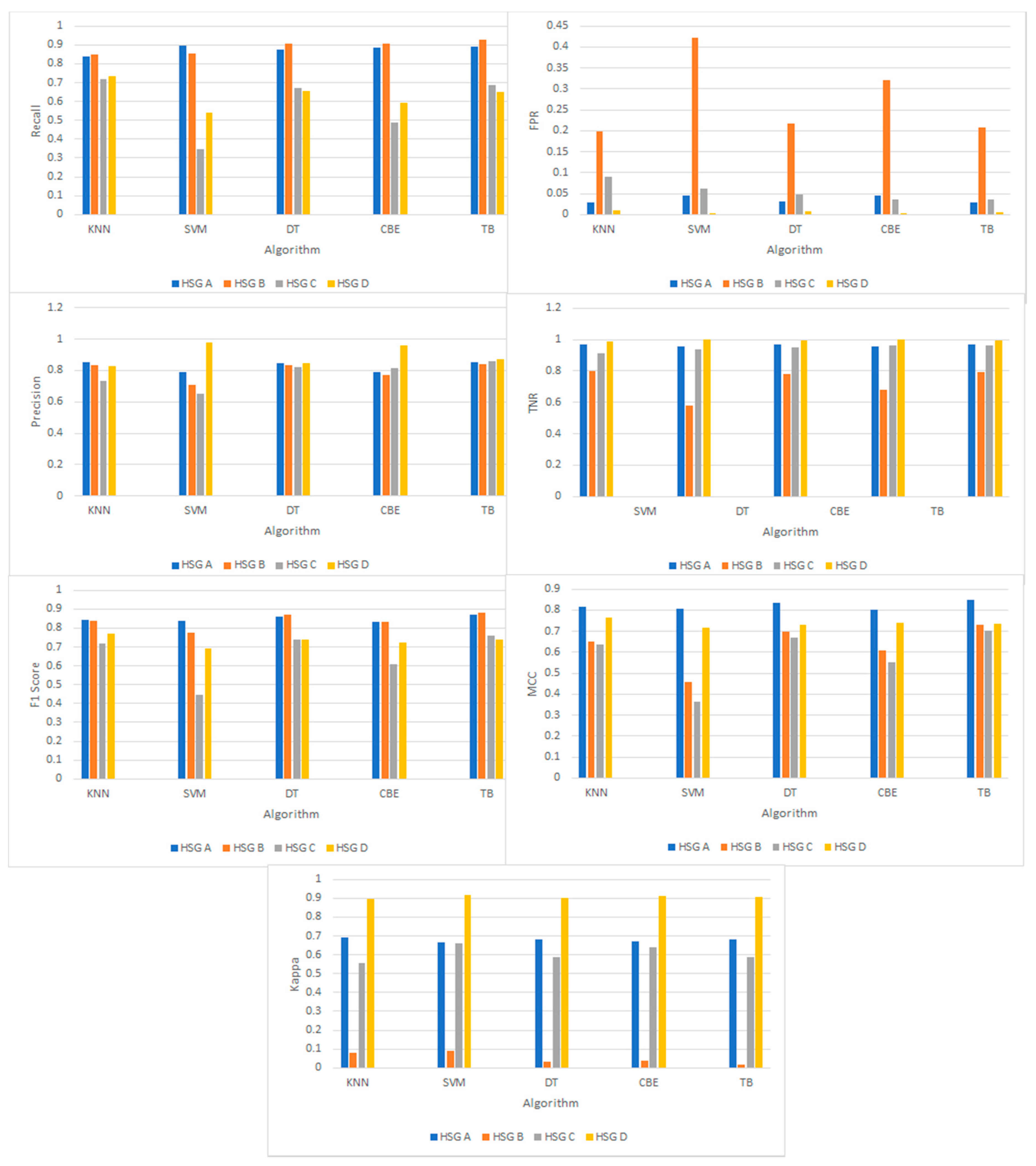
For datasets in which the classes are not represented equally (also known as imbalanced classes), accuracy is typically not a good measure of performance. Out of the 2107 unique soil samples in the observed group, 337 belong to HSG A, 1142 to HSG B, 511 to HSG C and 117 to HSG D. Given that our dataset is relatively imbalanced, we further evaluate the performance of all five algorithms based on metrics of Recall, Precision, FPR, TNR, F1-Score, MCC and Kappa. It is important to account for chance agreement when dealing with highly imbalanced classes since a high classification accuracy could result from classifying all observations as the largest class [35,36]. Table 3 lists per-class results and macro- and micro-averages of these metrics for classification using kNN, SVM and Decision Trees. Table 4 presents the same for two Ensemble Learning algorithms. A graphical comparison of individual classes (HSGs) for each metric is shown in Figure 3.
It should be noted that micro-averages for Recall, Precision and F1-Sscore are equal, as expected in multi-class classification problems. Moreover, micro-averages for MCC and Kappa are equal. It can be observed that for all five algorithms, the ability of the classifiers to correctly predict (Recall) HSGs A and B are relatively higher when compared to HSGs C and D. This is in line with results obtained for three-class and seven-class classification of soil types using Decision Trees and SVM in [19], wherein sandy soils had higher classification accuracy. On the other hand, the certainty with which the classifiers predict correct classes (Precision) is relatively higher for HSG D in our work. A comparison of macro- and micro-averages of F1-Scores among the five classifiers shows that kNN, Decision Tree and TreeBagger have scores close to 0.8, while SVM-Gaussian Kernel lags with a score close to 0.7. Among the four soil groups, HSG B has the highest rate of False Positives, with the highest being 57.8 percent for SVM-Gaussian Kernel and lowest being 19.83 percent for kNN. The fact that HSG B is the largest class in the dataset, and bordered by two other groups, explains the high FPR. A comparison of macro- and micro-averages of MCCs among the five classifiers shows comparable results (~0.72) for kNN, Decision Tree and TreeBagger. Yet again, SVM-Gaussian kernel has the lowest score (~0.6). The results of Cohen’s Kappa coefficient for HSG B shows some discrepancy that is consistent across all five classifiers. This may be related to the corresponding high FPRs. Regardless, the micro-average Kappa value is consistent with that of MCC, possibly accounting for any class imbalance. An interesting observation is that the micro- and macro-averages of Kappa coefficients for all five classifiers are similar in value. The macro-averages range from 0.55 (RF and DT) to 0.58 (SVM) and micro-averages range from 0.65 (SVM) to 0.73 (kNN and CBE), all within the moderate to substantial agreement range [37]. This similarity is observed in studies related to machine learning techniques for DSM, suggesting that the quality and robustness of datasets is of greater importance than the classifier itself [38,39]. In the context of predicting soil map units on tropical hillslopes in Brazil, an RF model yielded an overall accuracy of 78.8 percent and a Kappa index of 0.76, while a Decision Tree model had an overall accuracy of 70.2 percent and a Kappa value of 0.66 [39]. In contrast, for classification based on soil taxonomic units in British Columbia, Canada, kNN and SVM resulted in the highest accuracy of 72 percent; however, models such as CART with bagging and RF were preferred due to the speed of parameterization and the interpretability of the results, while resulting in similar accuracies ranging from 65 to 70 percent [40].
6. Conclusions
This work presents the application of machine learning towards classification of soil into hydrologic groups. The machine learning models tested were kNN, SVM-Gaussian Kernel, Decision Trees and Ensemble Learning (Classification Bagged Ensemble and Random Forest). It was observed that for all five classifiers, Recall for HSGs A and B were relatively higher when compared to HSGs C and D, but precision was relatively higher for HSG D. Overall, performance metrics related to kNN, Decision Tree and TreeBagger exceeded those for SVM-Gaussian Kernel and Classification Bagged Ensemble.
As part of future work, the effects of class imbalance will be investigated by comparing datasets with varying degrees of imbalance and using various cross-validation techniques with proportional stratified random sampling. Deep learning methods that address this classification problem will also be explored.
Author Contributions
Conceptualization, S.A.; methodology, S.A.; software, S.A., C.H. and H.V.; validation, S.A., C.H. and H.V.; formal analysis, S.A., C.H. and H.V.; investigation, S.A., C.H. and H.V.; resources, S.A.; data curation, S.A., C.H. and H.V.; writing—original draft preparation, S.A.; writing—review and editing, S.A., C.H. and H.V.; visualization, S.A., C.H. and H.V.; supervision, S.A.; project administration, S.A.; funding acquisition, S.A. All authors have read and agreed to the published version of the manuscript.
Funding
This research was funded by W.M. Keck Foundation through the Undergraduate Education Grant Program.
Conflicts of Interest
The authors declare no conflict of interest.
References
- Huffman, R.L.; Fangmeier, D.D.; Elliot, W.J.; Workman, S.R. Infiltration and Runoff. In Soil and Water Conservation Engineering, 7th ed.; American Society of Agricultural Engineers: St. Joseph, MI, USA, 2013; pp. 81–113. [Google Scholar]
- Kokkonen, T.; Koivusalo, H.; Karvonen, T. A Semi-Distributed Approach to Rainfall-Runoff Modelling—A Case Study in a Snow Affected Catchment. Environ. Model. Softw. 2001, 16, 481–493. [Google Scholar] [CrossRef]
- Hydrology Training Series: Module 104-Runoff Curve Number Computations. Available online: https://www.wcc.nrcs.usda.gov/ftpref/wntsc/H&H/training/runoff-curve-numbers1.pdf (accessed on 12 December 2018).
- Musgrave, G.W. How Much of the Rain Enters the Soil? In Water: U.S. Department of Agriculture Yearbook; United States Government Publishing Office (GPO): Washington, DC, USA, 1995; pp. 151–159. [Google Scholar]
- United States Department of Agriculture. Chapter 7: Hydrologic Soil Groups. In Part 630 Hydrology, National Engineering Handbook; 2009. Available online: https://directives.sc.egov.usda.gov/viewerFS.aspx?id=2572 (accessed on 10 December 2018).
- Morris, D.K.; Stienhardt, G.C.; Nielsen, R.L.; Hostetter, W.; Haley, S.; Struben, G.R. Using GPS, GIS, and Remote Sensing as a Soil Mapping Tool. In Proceedings of the 5th International Conference on Precision Agriculture, Bloomington, IN, USA, 16–19 July 2000. [Google Scholar]
- Usery, E.L.; Pocknee, S.; Boydell, B. Precision farming data management using geographic information systems. Photogramm. Eng. Remote. Sens. 1995, 61, 1383–1391. [Google Scholar]
- Lagacherie, P.; McBratney, A.B.; Voltz, M. (Eds.) Digital Soil Mapping: An Introductory Perspective; Elsevier: Amsterdam, The Netherlands, 2007; Volume 31, pp. 3–24. [Google Scholar]
- McBratney, A.B.; Mendonça-Santos, M.L.; Minasny, B. On digital soil mapping. Geoderma 2003, 117, 3–52. [Google Scholar] [CrossRef]
- Carré, F.; McBratney, A.B.; Mayr, T.; Montanarella, L. Digital soil assessments: Beyond DSM. Geoderma 2007, 142, 69–79. [Google Scholar] [CrossRef]
- Arrouyas, D.; McKenzie, N.; Hempel, J.; de Forges, A.R.; McBratney, A.B. GlobalSoilMap: Basis of the Global Spatial Soil Information System; Taylor and Francis: London, UK, 2014. [Google Scholar]
- Runoff Curve Number Method: Beyond the Handbook. Available online: https://www.wcc.nrcs.usda.gov/ftpref/wntsc/H&H/CNarchive/CNbeyond.doc (accessed on 15 June 2019).
- Neilsen, R.D.; Hjelmfelt, A.T. Hydrologic Soil-Group Assignment. In Proceedings of the International Water Resources Engineering Conference, Reston, VA, USA, 3–7 August 1998. [Google Scholar]
- Li, R.; Rui, X.; Zhu, A.-X.; Liu, J.; Band, L.E.; Song, X. Increasing Detail of Distributed Runoff Modeling Using Fuzzy Logic in Curve Number. Environ. Earth Sci. 2015, 73, 3197–3205. [Google Scholar] [CrossRef]
- Samuel, A.L. Some studies in machine learning using the game of checkers. IBM J. research dev. 1959, 3, 210–229. [Google Scholar] [CrossRef]
- Mitchell, T.M. Machine Learning, 1st ed.; McGraw-Hill, Inc.: New York, NY, USA, 1997; p. 2. [Google Scholar]
- Illés, G.; Kovács, G.; Heil, B. Comparing and Evaluating Digital Soil Mapping Methods in a Hungarian Forest Reserve. Can. J. Soil Sci. 2011, 91, 615–626. [Google Scholar] [CrossRef]
- Behrens, T.; Schmidt, K.; MacMillan, R.A. Multi-Scale Digital Soil Mapping with Deep Learning. Sci. Rep. 2018, 8, 15244. [Google Scholar] [CrossRef] [Green Version]
- Bhattacharya, B.; Solomatine, D. Machine learning in soil classification. Neural Netw. 2006, 19, 186–195. [Google Scholar] [CrossRef]
- Tayfur, G.; Singh, V.P.; Moramarco, T.; Barbetta, S. Flood Hydrograph Prediction Using Machine Learning Methods. Water 2018, 10, 968. [Google Scholar] [CrossRef] [Green Version]
- Yang, M.; Xu, D.; Chen, S.; Li, H.; Shi, Z. Evaluation of Machine Learning Approaches to Predict Soil Organic Matter and pH Using vis-NIR Spectra. Sensors 2019, 19, 263. [Google Scholar] [CrossRef] [PubMed] [Green Version]
- Forkuor, G.; Hounkpatin, O.K.; Welp, G.; Thiel, M. High Resolution Mapping of Soil Properties Using Remote Sensing Variables in South-Western Burkina Faso: A Comparison of Machine Learning and Multiple Linear Regression Models. PLoS ONE 2017, 12, e0170478. [Google Scholar] [CrossRef] [PubMed]
- Silva, B.P.C.; Silva, M.L.N.; Avalos, F.A.P.; Menezes, M.D.d.; Curi, N. Digital soil mapping including additional point sampling in Posses ecosystem services pilot watershed, southeastern Brazil. Sci. Rep. Nat. 2019, 9, 13763. [Google Scholar]
- Wösten, J.H.M.; Pachepsky, Y.A.; Rawls, W.J. Pedotransfer functions: Bridging the gap between available basic soil data and missing soil hydraulic characteristics. J. Hydrol. 2001, 251, 123–150. [Google Scholar] [CrossRef]
- Abdelbaki, A.M.; Youssef, M.A.; Naguib, E.M.F.; Kiwan, M.E.; El-giddawy, E.I. Evaluation of Pedotransfer Functions for Predicting Saturated Hydraulic Conductivity for U.S. Soils. In Proceedings of the American Society of Agricultural and Biological Engineers Annual International Meeting, Reno, NV, USA, 21–24 June 2009. [Google Scholar]
- Araya, S.N.; Ghezzehei, T.A. Using machine learning for prediction of saturated hydraulic conductivity and its sensitivity to soil structural perturbations. Water Resour. Res. 2019, 55, 5715–5737. [Google Scholar] [CrossRef]
- Natural Resources Conservation Service Web Soil Survey. Available online: https://websoilsurvey.sc.egov.usda.gov/App/HomePage.htm (accessed on 10 November 2018).
- Natural Resources Conservation Service Soil Texture Calculator. Available online: https://www.nrcs.usda.gov/wps/portal/nrcs/detail/soils/survey/?cid=nrcs142p2_054167 (accessed on 10 November 2018).
- Hong, Y.; Adler, R.F. Estimation of global SCS curve numbers using satellite remote sensing and geospatial data. Int. J. Remote. Sens. 2008, 29, 471–477. [Google Scholar] [CrossRef]
- Urban Hydrology for Small Watersheds, Technical Release 55. Available online: www.nrcs.usda.gov/downloads/ hydrology_hydraulics/tr55/tr55.pdf (accessed on 15 June 2019).
- Xu, Q.S.; Liang, Y.Z. Monte Carlo cross validation. Chemom. Intell. Lab. Syst. 2001, 56, 1–11. [Google Scholar] [CrossRef]
- Knox, S.W. Machine Learning: A Concise Introduction; John Wiley & Sons Inc.: Hoboken, NJ, USA, 2018. [Google Scholar]
- Bell, J. Machine Learning: Hands-On for Developers and Technical Professionals; John Wiley & Sons Inc.: Hoboken, NJ, USA, 2014. [Google Scholar]
- Kruger, F. Activity, Context, and Plan Recognition with Computational Causal Behavior Models. Ph.D. Thesis, University of Rostock, Mecklenburg, Germany, 2016. Available online: https://pdfs.semanticscholar.org/bebf/183d2f57f79b5b3e85014a9e1d6392ad0e5c.pdf (accessed on 10 June 2019).
- Brungard, C.W.; Boettinger, J.L.; Duniway, M.C.; Wills, S.A.; Edwards, T.C., Jr. Machine learning for predicting soil classes in three semi-arid landscapes. Geoderma 2015, 239, 68–83. [Google Scholar] [CrossRef] [Green Version]
- Congalton, R.G.; Green, K. Assessing the Accuracy of Remotely Sensed Data: Principles and Practices; CRC/Taylor & Francis: Boca Raton, FL, USA, 1998. [Google Scholar]
- Landis, J.R.; Koch, G.G. The measurement of observer agreement for categorical data. Biometrics 1977, 33, 159–174. [Google Scholar] [CrossRef] [Green Version]
- Meier, M.; de Souza, E.; Francelino, M.; Filho, E.I.F.; Schaefer, C.E.G.R. Digital Soil Mapping Using Machine Learning Algorithms in a Tropical Mountainous Area. Revista Brasileira de Ciência do Solo 2018, 42, 1–22. [Google Scholar] [CrossRef] [Green Version]
- Chagas, C.S.; Pinheiro, H.; Carvalho, W.; Anjos, L.H.C.; Pereira, N.R.; Bhering, S.B. Data mining methods applied to map soil units on tropical hillslopes in Rio de Janeiro, Brazil. Geoderma Reg. 2016, 9, 47–55. [Google Scholar] [CrossRef]
- Heung, B.; Ho, H.C.; Zhang, J.; Knudby, A.; Bulmer, C.; Schmidt, M. An overview and comparison of machine-learning techniques for classification purposes in digital soil mapping. Geoderma 2016, 265, 62–77. [Google Scholar] [CrossRef]
Figure 1.
The soil textural triangle is used to determine soil textural class from the percentages of sand, silt and clay in the soil [28].
Figure 1.
The soil textural triangle is used to determine soil textural class from the percentages of sand, silt and clay in the soil [28].

Figure 2.
Confusion matrix for a multi-class model with N classes [34].
Figure 2.
Confusion matrix for a multi-class model with N classes [34].

Figure 3.
A graphical representation of per-class performance metrics for kNN, SVM-Gaussian Kernel, Decision Trees and Ensemble Learning Algorithms (CBE and TB).
Figure 3.
A graphical representation of per-class performance metrics for kNN, SVM-Gaussian Kernel, Decision Trees and Ensemble Learning Algorithms (CBE and TB).


| Relationship between Sand, Silt and Clay Percentages | Textural Class | Hydrologic Soil Group |
|---|---|---|
| ((silt + 1.5 * clay) < 15) | SAND | A |
| ((silt + 1.5 * clay ≥ 15) AND (silt + 2 * clay < 30)) | LOAMY SAND | A |
| ((clay ≥ 7 && clay < 20) AND (sand > 52) AND ((silt + 2 * clay) ≥ 30) OR (clay < 7 && silt < 50 AND (silt + 2 * clay) ≥ 30)) | SANDY LOAM | A |
| ((clay ≥ 7 AND clay < 27) AND (silt ≥ 28 AND silt < 50) AND (sand ≤ 52)) | LOAM | B |
| ((silt ≥ 50 AND (clay ≥ 12 AND clay < 27)) OR ((silt ≥ 50 AND silt < 80) AND clay < 12)) | SILT LOAM | B |
| (silt ≥ 80 AND clay < 12) | SILT | B |
| ((clay ≥ 20 AND clay < 35) AND (silt < 28) AND (sand > 45)) | SANDY CLAY LOAM | C |
| ((clay ≥ 27 AND clay < 40) AND (sand > 20 AND sand ≤ 45)) | CLAY LOAM | D |
| ((clay ≥ 27 AND clay < 40) AND (sand ≤ 20)) | SILTY CLAY LOAM | D |
| (clay ≥ 35 AND sand > 45) | SANDY CLAY | D |
| (clay ≥ 40 AND silt ≥ 40) | SILTY CLAY | D |
| clay ≥40 AND sand ≤ 45 AND silt < 40 | CLAY | D |
Table 2.
Comparison of overall accuracy.
| Method | Overall Accuracy |
|---|---|
| Soil Texture Calculator | 0.54 |
| k-Nearest Neighbor (kNN) | 0.81 |
| SVM Gaussian Kernel | 0.72 |
| Decision Tree | 0.83 |
| Classification Bagged Ensemble | 0.79 |
| TreeBagger | 0.85 |
Table 3.
Comparison of performance metrics for classification using k-Nearest Neighbors (kNN), Support Vector Machine (SVM) and decision trees.
Table 3.
Comparison of performance metrics for classification using k-Nearest Neighbors (kNN), Support Vector Machine (SVM) and decision trees.
| k-Nearest Neighbor (kNN); k = 4 | |||||||
| Recall | Precision | FPR | TNR | F1 Score | MCC | Kappa | |
| HSG A | 0.84 | 0.86 | 0.03 | 0.97 | 0.84 | 0.82 | 0.69 |
| HSG B | 0.85 | 0.84 | 0.20 | 0.80 | 0.84 | 0.65 | 0.08 |
| HSG C | 0.72 | 0.73 | 0.09 | 0.91 | 0.72 | 0.63 | 0.56 |
| HSG D | 0.73 | 0.83 | 0.01 | 0.99 | 0.77 | 0.76 | 0.89 |
| Macro Average | 0.78 | 0.81 | 0.08 | 0.92 | 0.79 | 0.72 | 0.56 |
| Micro Average | 0.80 | 0.80 | 0.07 | 0.93 | 0.80 | 0.73 | 0.73 |
| Support Vector Machines (SVM) Gaussian Kernel | |||||||
| HSG A | 0.90 | 0.79 | 0.05 | 0.95 | 0.84 | 0.81 | 0.67 |
| HSG B | 0.86 | 0.71 | 0.42 | 0.58 | 0.77 | 0.46 | 0.09 |
| HSG C | 0.35 | 0.65 | 0.06 | 0.94 | 0.45 | 0.36 | 0.66 |
| HSG D | 0.54 | 0.98 | 0.00 | 1.00 | 0.69 | 0.72 | 0.91 |
| Macro Average | 0.66 | 0.78 | 0.13 | 0.87 | 0.69 | 0.59 | 0.58 |
| Micro Average | 0.74 | 0.74 | 0.09 | 0.91 | 0.74 | 0.65 | 0.65 |
| Decision Tree | |||||||
| HSG A | 0.88 | 0.84 | 0.03 | 0.97 | 0.86 | 0.83 | 0.68 |
| HSG B | 0.91 | 0.83 | 0.22 | 0.78 | 0.87 | 0.70 | 0.03 |
| HSG C | 0.67 | 0.82 | 0.05 | 0.95 | 0.74 | 0.67 | 0.59 |
| HSG D | 0.66 | 0.85 | 0.01 | 0.99 | 0.74 | 0.73 | 0.90 |
| Macro Average | 0.78 | 0.84 | 0.08 | 0.92 | 0.80 | 0.73 | 0.55 |
| Micro Average | 0.79 | 0.79 | 0.07 | 0.93 | 0.79 | 0.72 | 0.72 |
Table 4.
Comparison of performance metrics for classification using ensemble learning algorithms.
| Classification Bagged Ensemble | |||||||
| Recall | Precision | FPR | TNR | F1 Score | MCC | Kappa | |
| HSG A | 0.89 | 0.79 | 0.05 | 0.95 | 0.83 | 0.80 | 0.67 |
| HSG B | 0.91 | 0.77 | 0.32 | 0.68 | 0.83 | 0.61 | 0.04 |
| HSG C | 0.49 | 0.82 | 0.04 | 0.96 | 0.61 | 0.55 | 0.64 |
| HSG D | 0.59 | 0.96 | 0.00 | 1.00 | 0.73 | 0.74 | 0.91 |
| Macro Average | 0.72 | 0.83 | 0.10 | 0.90 | 0.75 | 0.68 | 0.57 |
| Micro Average | 0.79 | 0.79 | 0.07 | 0.93 | 0.79 | 0.73 | 0.73 |
| TreeBagger; N = 50 | |||||||
| HSG A | 0.89 | 0.85 | 0.03 | 0.97 | 0.87 | 0.85 | 0.68 |
| HSG B | 0.93 | 0.84 | 0.21 | 0.79 | 0.88 | 0.73 | 0.02 |
| HSG C | 0.69 | 0.86 | 0.04 | 0.96 | 0.76 | 0.71 | 0.59 |
| HSG D | 0.65 | 0.87 | 0.01 | 0.99 | 0.74 | 0.74 | 0.90 |
| Macro Average | 0.79 | 0.86 | 0.07 | 0.93 | 0.81 | 0.76 | 0.55 |
| Micro Average | 0.78 | 0.78 | 0.08 | 0.92 | 0.78 | 0.70 | 0.70 |
© 2019 by the authors. Licensee MDPI, Basel, Switzerland. This article is an open access article distributed under the terms and conditions of the Creative Commons Attribution (CC BY) license (http://creativecommons.org/licenses/by/4.0/).
Share and Cite
MDPI and ACS Style
Abraham, S.; Huynh, C.; Vu, H. Classification of Soils into Hydrologic Groups Using Machine Learning. Data 2020, 5, 2. https://0-doi-org.brum.beds.ac.uk/10.3390/data5010002
AMA Style
Abraham S, Huynh C, Vu H. Classification of Soils into Hydrologic Groups Using Machine Learning. Data. 2020; 5(1):2. https://0-doi-org.brum.beds.ac.uk/10.3390/data5010002
Chicago/Turabian StyleAbraham, Shiny, Chau Huynh, and Huy Vu. 2020. "Classification of Soils into Hydrologic Groups Using Machine Learning" Data 5, no. 1: 2. https://0-doi-org.brum.beds.ac.uk/10.3390/data5010002