An Optimum Tea Fermentation Detection Model Based on Deep Convolutional Neural Networks
by
 , , , and
Gibson Kimutai
1,* ,
,
Alexander Ngenzi
1,
Rutabayiro Ngoga Said
1,
Ambrose Kiprop
2,3 and
Anna Förster
4 1
African Center of Excellence in Internet of Things (ACEIoT), College of Science and Technology, University of Rwanda, P.O. Box, 3900 Kigali, Rwanda
2
Department of Chemistry and Biochemistry, Moi University, P.O. Box, 3900-30100 Eldoret, Kenya
3
African Center of Excellence in Phytochemicals, Textile and Renewable Energy (ACE II-PTRE), P.O. Box, 3900-30100 Eldoret, Kenya
4
Sustainable Communication Networks, University of Bremen, 8359 Bremen, Germany
*
Author to whom correspondence should be addressed.
Data 2020, 5(2), 44; https://0-doi-org.brum.beds.ac.uk/10.3390/data5020044
Submission received: 2 April 2020
/
Revised: 28 April 2020
/
Accepted: 28 April 2020
/
Published: 30 April 2020
(This article belongs to the Special Issue Machine Learning in Image Analysis and Pattern Recognition)
Abstract
:Tea is one of the most popular beverages in the world, and its processing involves a number of steps which includes fermentation. Tea fermentation is the most important step in determining the quality of tea. Currently, optimum fermentation of tea is detected by tasters using any of the following methods: monitoring change in color of tea as fermentation progresses and tasting and smelling the tea as fermentation progresses. These manual methods are not accurate. Consequently, they lead to a compromise in the quality of tea. This study proposes a deep learning model dubbed TeaNet based on Convolution Neural Networks (CNN). The input data to TeaNet are images from the tea Fermentation and Labelme datasets. We compared the performance of TeaNet with other standard machine learning techniques: Random Forest (RF), K-Nearest Neighbor (KNN), Decision Tree (DT), Support Vector Machine (SVM), Linear Discriminant Analysis (LDA), and Naive Bayes (NB). TeaNet was more superior in the classification tasks compared to the other machine learning techniques. However, we will confirm the stability of TeaNet in the classification tasks in our future studies when we deploy it in a tea factory in Kenya. The research also released a tea fermentation dataset that is available for use by the community.
1. Introduction
Tea is one of the most popular and lowest cost beverages in the world [1]. Currently, more than 3 billion cups of tea are consumed every day worldwide. This popularity is attributed to its health benefits, which include prevention of breast cancer [2], skin cancer [3], colon cancer [4], neurodegenerative complication [5], prostate cancer [6], and many others. Tea is also attributed to the prevention of diabetes and boosting metabolism [7]. Depending on the manufacturing technique, it may be described as green, black, oolong, white, yellow, and compressed tea [8]. Black tea accounts for approximately 70% of tea produced worldwide. The top four tea-producing countries are China, Sri Lanka, Kenya, and India (Table 1).
Kenya is the largest producer of black tea in the world [7] due to its low altitude, rich loamy soil conditions, ample rainfall, and a unique climate [9]. In Kenya, tea is produced by small- and large-scale farmers. Small-scale farmers are more than 562,000 and account for about 62% of the total tea produced in Kenya [10]. The rest are produced by large-scale tea plantations that operate 39 factories. Smallholder farmers are managed by the government through the Kenya tea development agency (KTDA) board [11]. The board manages 66 tea factories across the country where smallholder tea is processed [1]. Tea is regarded as a significant contributor to the country’s economy as it is the leading exchange earner and contributes to more than 4% of the gross domestic product (GDP). The sector is also a source of livelihoods to more than 10% of the country’s estimated population of 40 million people [12,13]. Despite the importance of tea to the country, the sector is facing a myriad of challenges which include high production cost, mismanagement, bad agricultural practices, climate change, market competition from other countries, low prices, and lack of automation, among others [13].
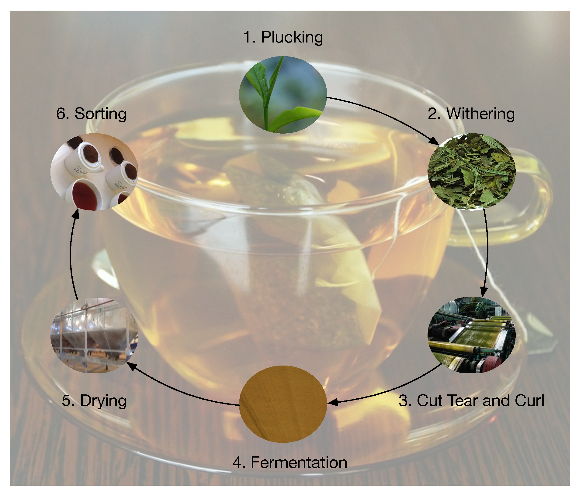
There are 5 steps in the production of black tea (Figure 1). The process starts with the plucking of green tea, where two leaves and a bud is the standard. The next step is withering, where tea leaves are spread on a withering bed for them to lose moisture.
There is then the cut, tear, and curl step, where tea leaves are cut and torn to open them up for oxidation. The fermentation stage is where tea reacts with oxygen to produce compounds that are responsible for the quality of tea. Heat is passed through tea in the drying stage to remove moisture. The last step is sorting where tea is put into various categories based on their quality. Out of these steps, fermentation is the most important in determining the quality of tea produced [14].
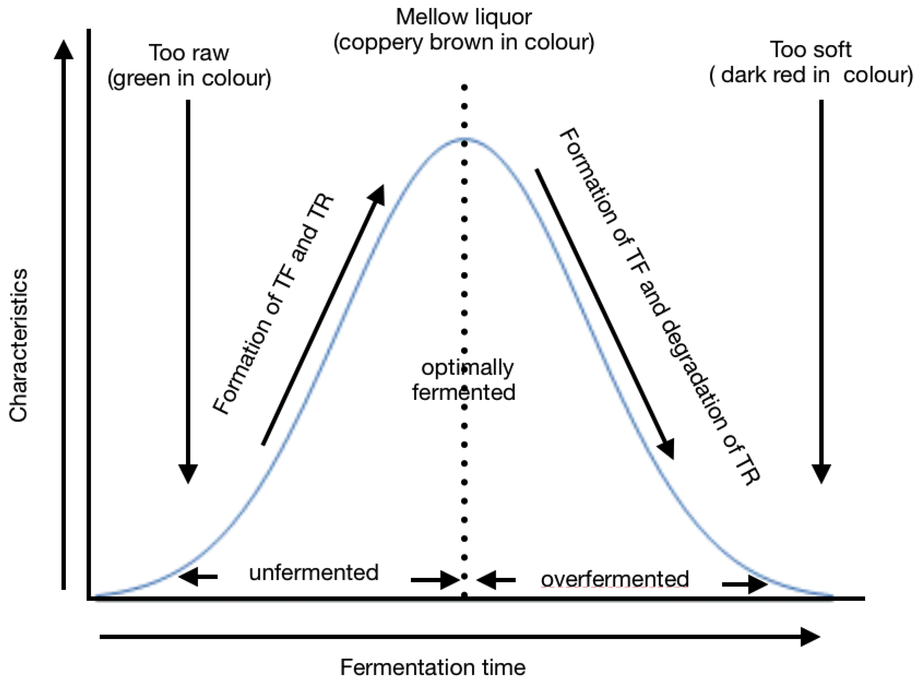
The fermentation process begins when cells of ruptured tea leaves react with oxygen to produce two compounds: Theaflavins (TF) and Thearubins (TR) [15,16]. Theaflavins are responsible for the brightness and briskness of the tea liquor while TR is responsible for the color, taste, and body of tea [16]. During fermentation, the following parameters must be maintained: temperature, relative humidity, and time [15]. The optimum temperature under which fermentation should take place should be approximately 25 °C. The ideal humidity should be approximately 42% [17]. Fermentation is a time-bound process (Figure 2); at the beginning, the liquor is raw and with a green infusion. The formation of TF and TR increases with time until optimum fermentation is achieved. At the optimum fermentation time, the liquor is mellow and with a bright infusion. This is the desired point in fermentation. After optimum fermentation time, the formation of TR reduces and degradation of TF begins. This stage is over-fermentation, where the liquor is soft and with a dark infusion.
Currently, tea tasters determine optimum fermentation manually by either of the following methods: smell peaks, color change, infusion, or tasting of tea. The constant intervention of humans in a fermentation room disturbs the environment created for fermentation and is also unhygienic. Moreover, humans are subjective and prone to error [7]. These manual methods lead to a compromise in the quality of produced tea and translate to low prices of tea. Therefore, there is a need for alternative means of monitoring the process of fermentation which is the focus of this research.
Currently, machine learning has been applied to many different fields: engineering, science, education, medicine, business, accounting, finance, marketing, economics, stock market, and law, among others [18,19,20,21,22]. Machine Learning (ML) is a branch of artificial intelligence (AI) that enables a system to learn from concepts and knowledge [23]. Deep learning is a collection of machine learning algorithms which models high-level abstractions in data with nonlinear transformations [24]. Deep learning works with the principle of the Artificial Neural Networks (ANN) system, and its fundamental computation unit is a neuron [19,24,25]. In ML, feature extraction and classification are in different steps, while in deep learning, they are in a single step and are done concurrently.
The contribution of this paper is twofold: First, this research proposes a deep learning model based on CNN for monitoring black tea during fermentation. Secondly, this research releases a tea fermentation dataset [26]. The rest of the paper is arranged as follows: presentation of some of the studies aimed at digitizing fermentation is done in Section 2 and a discussion of materials and methods used in this research is presented in Section 3. We provide implementation of the models and the evaluation metrics in Section 4, while Section 5 provides the results and their discussions. We conclude the study in Section 6.
2. Related Work
With advancements in computing, digitization across many fields is being witnessed [27]. In agriculture, tea processing has been receiving attention from researchers. Proposals have been made on improving the detection of optimum fermentation using the following techniques: electronic nose, electronic tongue, and machine vision. An electronic nose is a smart instrument designed to detect and discriminate odors using sensors [28]. The basic elements of an electronic nose are an odor sensor and an actuator. Proposals to use the electronic nose in detecting optimum tea fermentation have been proposed in References [14,29,30,31,32]. In Reference [31], a handheld electronic nose is proposed, while in Reference [32], ultra-low power techniques have been incorporated into an electronic nose. From the literature, it is evident that the electronic nose has made technological breakthroughs. However, they have not been implemented in many tea factories due to its high price and since they are power-hungry. Going into the future, adoption of the electronic nose will depend on innovative ways of using low-cost sensors in their design. It will also depend on the ability to apply ultra-low-power power design techniques to minimize power consumption.
Some studies exist on the application of an electronic tongue to monitor tea fermentation. They include References [33,34,35,36]. In Reference [33], an optimal fermentation model with the use of electronic nose and machine learning techniques is proposed. In Reference [34], the authors applied CNN in the development of an electronic tongue. In Reference [37], an electronic tongue to monitor biochemical changes during tea fermentation is proposed. The authors in Reference [35] designed an electronic tongue for testing the quality of fruits. Research in Reference [36] proposes an electronic tongue with the use of a KNN algorithm and adaptive boosting for development. A fusion of the electronic nose and electronic tongue technologies has been proposed in Reference [38]. It is evident from the literature that there have been proposals to use the electronic tongue in detecting optimal fermentation. However, they have not been implemented in tea factories because these technologies are power-hungry and expensive.
The rapid development of computer vision technology in recent years has led to an increased usage of computational image processing and recognition methods. Proposals to apply image processing in the fermentation of tea are reported in References [39,40,41,42,43,44]. Research in Reference [39] proposes a quality indexing model for black tea during fermentation using image processing techniques. Another remarkable research is in Reference [40], which detects changes in color during fermentation. In Reference [41], artificial neural networks (ANN) and image processing techniques are applied to detect color changes of tea during fermentation. Research in Reference [42] applied SVM with image processing to detect optimum tea fermentation. In Reference [43], the authors used image processing to detect the color change of tea during fermentation. The authors in Reference [44] implemented an electronic tongue with machine vision to predict the optimum fermentation of black tea. From the literature, tea fermentation is an active research area with authors suggesting different approaches. However, the tea fermentation dataset has not to be used. The use of image processing is the most viable approach due to the low cost of imaging devices. Additionally, a color change is easy to detect compared to taste and odor.
3. Materials and Methods
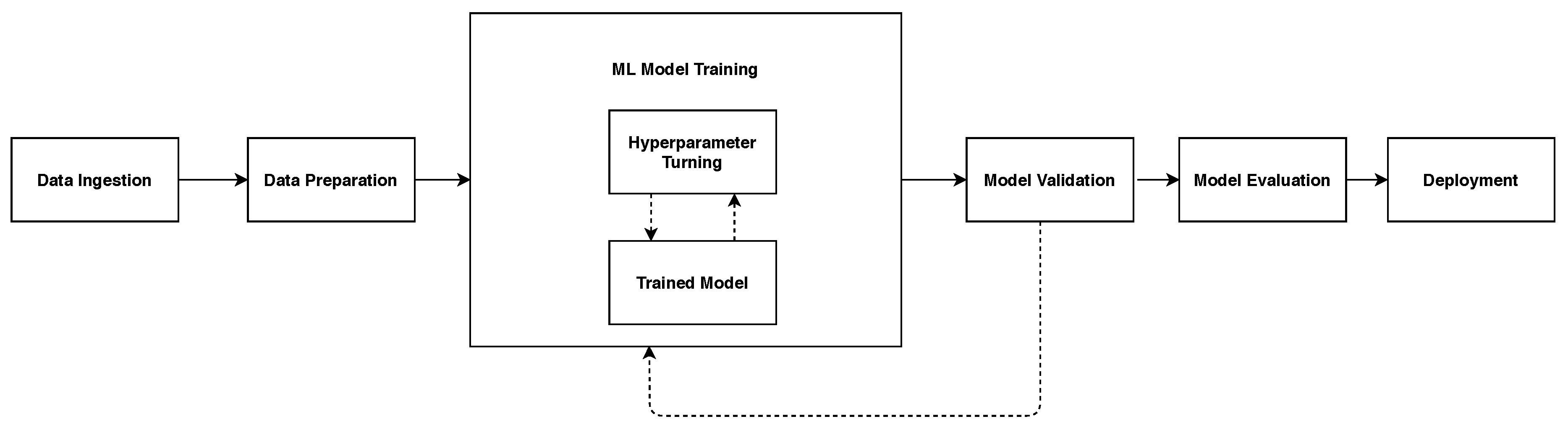
After acquiring data, the next phase was data preprocessing where activities discussed in Section 3.2 were done. The cleaned data was fed to the ML classifiers for training (Figure 3). The training involved hyperparameter tuning until the models were fully trained. Some of the hyperparameters are the learning rate, number of the epoch, regularization coefficient, and batch size. Currently, the available optimization strategies include grid search, random search, hill-climbing, and bayesian optimization, among others [45]. In this study, we adopted the grid search and random search methods. The models were then validated and evaluated using the data discussed in Section 3.1.
In model validation, models which did not pass the validation tests were taken back to the training phase. The evaluation results are presented in Section 5. The models can be deployed to a tea fermentation environment after the aforementioned steps.
This section discusses the datasets used, data preprocessing steps, feature extraction methods, machine learning classification models, and the proposed deep learning model.
3.1. Datasets
In this paper, two datasets were used: tea fermentation and LabelMe datasets. Since there was no existing standard dataset on tea fermentation images existing in the community, we used the LabelMe dataset to validate our results for it is widely used by researchers in image classification to report their results, the dataset is available at no cost, and there was no available dataset on images of tea fermentation images. We discuss each of the datasets in the following paragraphs.
3.1.1. Tea Fermentation Dataset
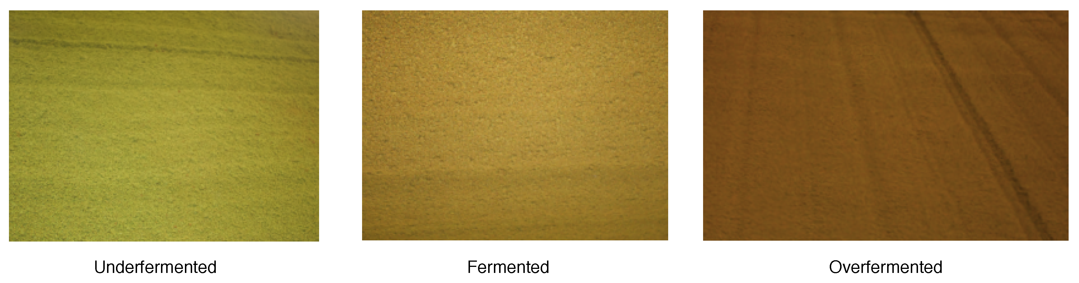
The images in the tea fermentation dataset [26] were taken in a black tea fermentation environment in a tea factory in Kenya. We used a 5-megapixel camera connected to a Raspberry Pi 3 model B+ to capture the images. Fermentation dataset contains 6000 images that were captured during the fermentation of black tea. Figure 4 shows an image of each of the classes of the tea fermentation dataset. The classes of the images in this dataset are: underfermented, fermented, and overfermented.
Table 2 shows the number of images for every class that was used as training, validation, and testing datasets for the classification algorithms. The 80/20 ratio of training/test data is the most commonly used ratio in neural network applications and was adopted in this research. Besides, 10% subset of the test dataset was used to validate the results. A total of 4800 images distributed equally to the 3 classes of images were used for training of the models. To perform validation, 40 images were used in each of the classes while 360 images were used to test the model in each of the 3 classes.
3.1.2. LabelMe Dataset
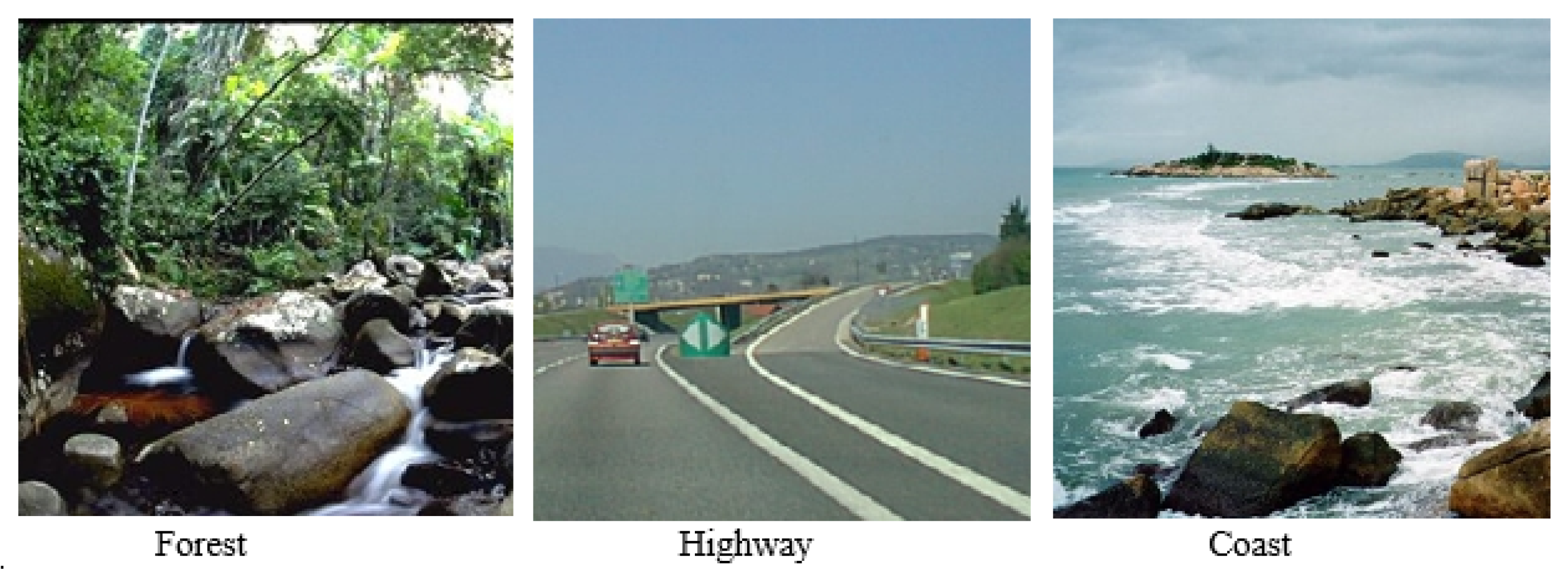
As explained in Section 3.1, the other dataset that we adopted in this study is the LabelMe dataset [46]. The dataset is one of the standard datasets which researches in the field of image classification use to report their results. The dataset contains 2688 images from 3 classes of outdoor scenes. The classes are forest, coast, and highway. Examples of images from each of the classes are shown in Figure 5.
Table 3 shows the number of images used for training, validation, and testing in each of the categories. As with the case in Section 3.1.1, we adopted the 80/20 ratio for training and testing and 10% for validation.
3.2. Data Preprocessing and Augmentation
After collecting the images as discussed in Section 3.1.1, the images were resized to 150 × 150. Resizing images to 150 × 150 before inputting them into different networks was done to adapt different pretraining CNN structures. We adopted the semantic segmentation annotation method discussed in Reference [47] to annotate the images. There are numerous types of noise in images but the most common are photon noise, readout noise, and dark noise [48,49]. To perform denoising, we adopted the linear filtering method.
3.3. Feature Extraction
Feature extraction in image processing is the process of extracting image features. It is the most crucial step in image classification as it directly affects perfomance of the classifiers [50]. There are various techniques of feature extraction, but in this paper, we adopted color histogram for color feature extraction and Local Binary Patterns (LBP) algorithm for texture extraction.
3.3.1. Color Feature Extraction
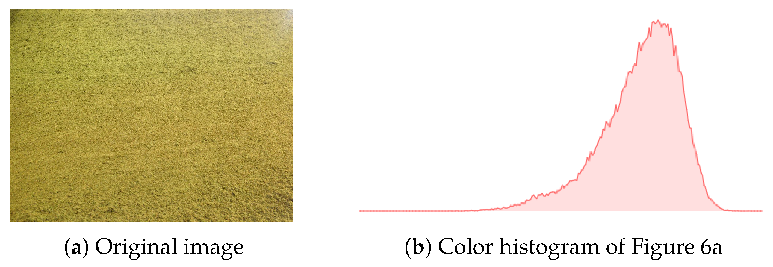
Color is an important feature descriptor of an image. During tea fermentation, the color change is evident as the process continues. Relative color histograms in different color spaces can be used to describe tea fermentation images. There are several color spaces which include Red-green Blue (RGB), Hue Saturation Value (HSV), and Hue Saturation Brightness (HSB), among others [51,52,53,54]. RGB color space represents a mixture of red, green, and blue. This is the color space that was used to represent the images in this paper. We used color histogram [55] to extract color features of the images that are then fed to the classifiers for training, evaluation, and testing. To construct a feature vector from the color histogram, we used OpenCV [56]. The input was an image of RGB color space. The RGB color space was converted to HSV and represented by 3 channels (the hue, the saturation, and the value). We used 8 bins to represent the three channels. Finally, the range of the channels was between 0–150 since the images had been resized to 150 by 150 pixels. Figure 6a shows an image of underfermented tea, while Figure 6b shows the corresponding color histogram.
3.3.2. Texture Feature Extraction
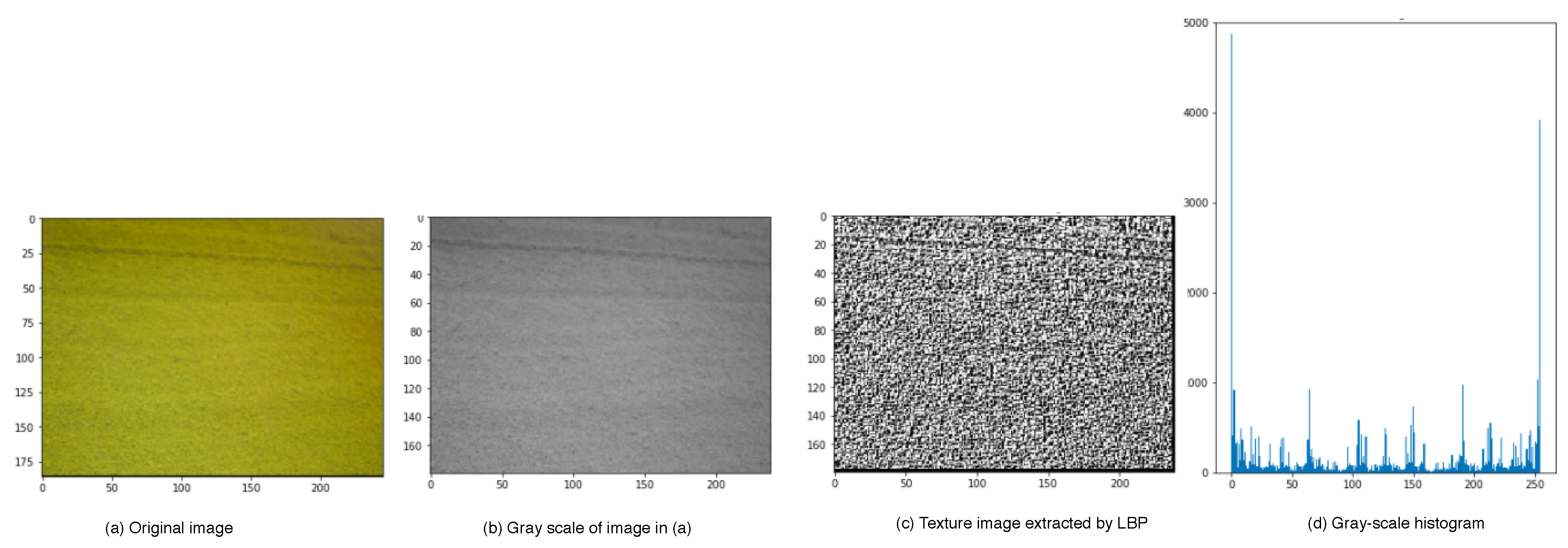
Textures are characteristic intensity variations that originate from the roughness of an object surface. The texture of an image is classified into first-order, second-order, and higher-order statistics [57]. There are a variety of methods of extracting texture features including Local Binary Patterns (LBP), the Canny edge detection, discrete wavelet transform, and gray level occurrence matrix, among others [58,59,60]. In this paper, we adopted LBP to extract the texture features of the images. LBP has many advantages which include reduced histograms and consideration of the center pixels point effect [61], among others. The LBP algorithm is represented by Equation (1):
where LBP xc,yc is the value at the center pixel xc,yc, In is the values of neighbor pixel, and I(xc, yc) is the intensity at the center pixel.
The steps of the texture feature extraction were as follows:
- Finally, the texture image obtained was converted into gray- scale histogram as shown in Figure 7d.
3.4. Classification Models
In this paper, we perform the classification of the images in the datasets discussed in Section 3.1 using the following classifiers: decision tree, random forest, K- nearest neighbor, TeaNet, support vector machine, linear discriminant analysis, and naive Bayes. The next paragraphs discuss each of the classifiers.
3.4.1. Decision Tree (DT)
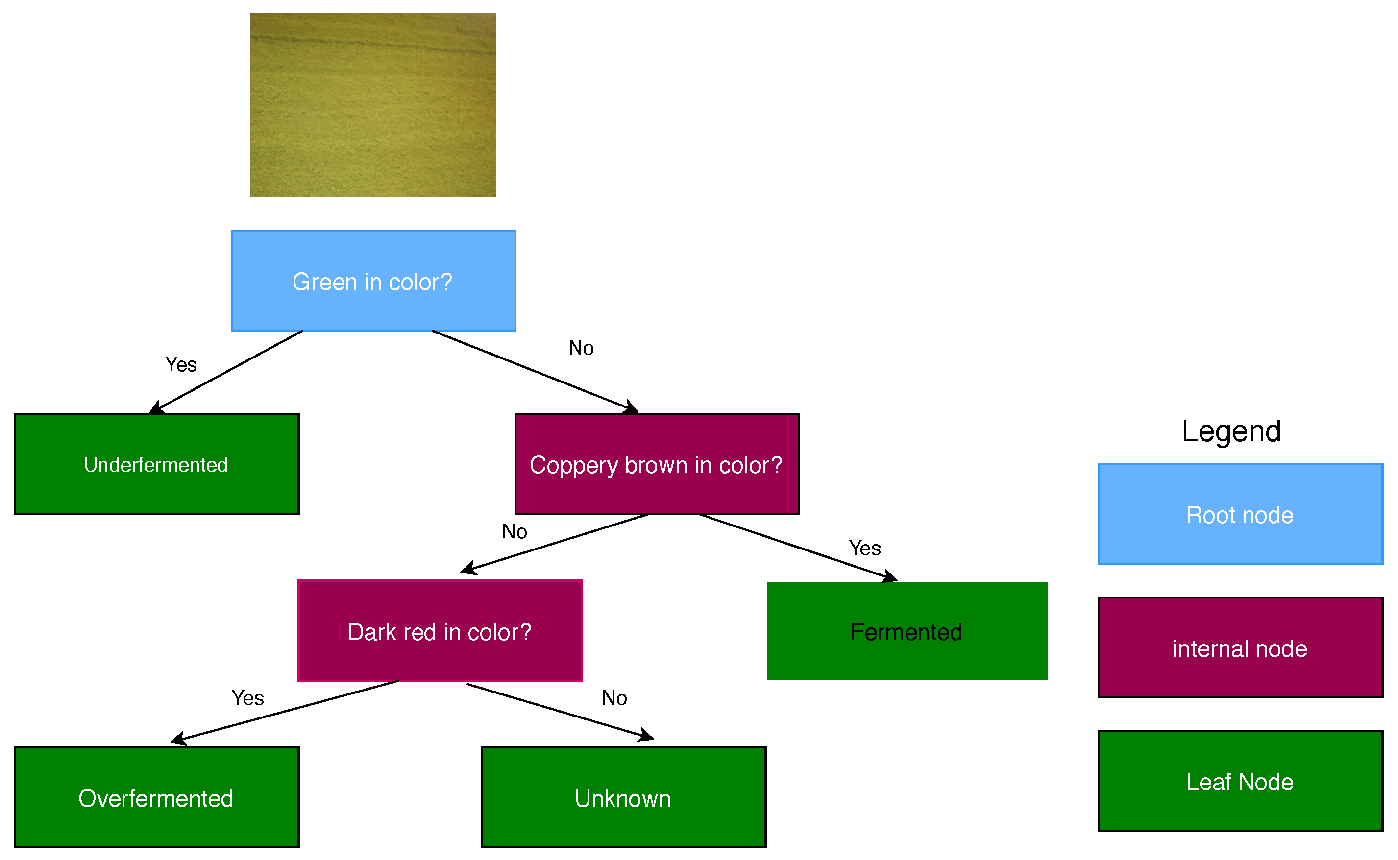
Decision tree is a machine learning technique that employs a tree structure to specify the order of the decisions and the consequences [63]. During training, it generates rules and decision trees. The generated DTs are followed in the classification of the new data [64]. It has the following constituents: root node, internal node, and leaf node (Figure 8). Branches and leaves point to the factors that concern a particular situation [65].
It is one of the most used machine learning algorithms in classification [66,67] because of its advantages which include high tolerance to multicollinearity [68], flexibility, and exclusion of factors which are not important automatically [63,69], among others. However, DT training is relatively expensive as complexity and time taken are more, a small change in data changes the DT structure, and it is inadequate in predicting continuous values, among others [70].
3.4.2. Random Forest (RF)
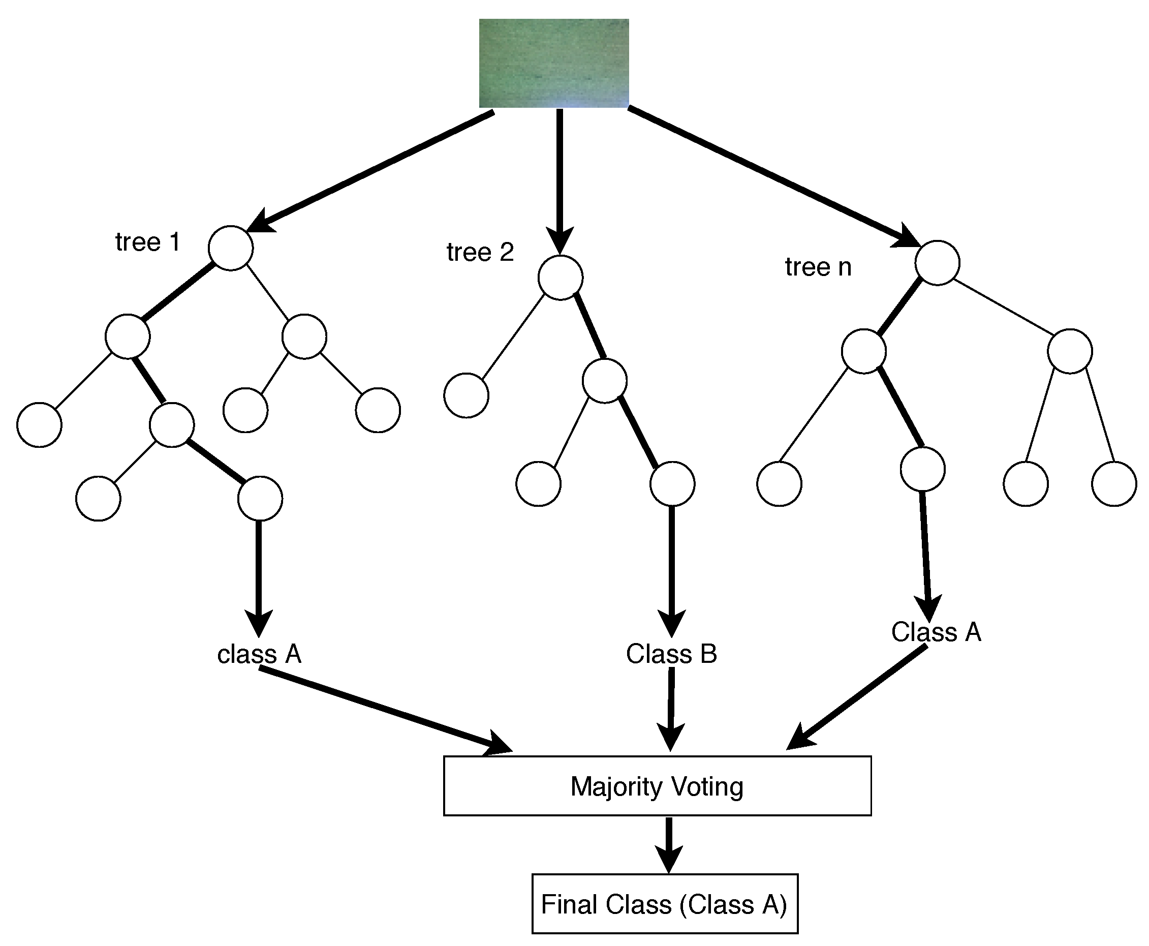
Random forest is a machine learning model that operates by constructing multiple decision trees during training [71,72]. The constructed multiple trees are then used for prediction during classification. Each individual tree in the random forest outputs a class prediction and the class with most votes becomes the model’s prediction [73]. Figure 9 shows an example of classifying an image using random forest. The image was classified as belonging to class A since the majority of the trees (2) classified the image as belonging to class A. The classifier can estimate missing data, can balance errors in datasets where classes are imbalanced, and can be used for both classification and regression [74,75,76,77]. Additionally, it has better results compared to decision tree algorithm; the random forest has a better classification result [72,78]. However, random forest is not as effective in regression tasks as it is in classification and is a black box model [79,80,81].
3.4.3. K-Nearest Neigbor (KNN)
K-Nearest Neighbor (KNN) is a nonparametric machine learning model used for classification and regression [82,83,84]. In classification tasks, KNN determines the class of a new sample based on the class of its nearest neighbors. During decision making in a classification task, it finds k training instances that are closest to the unknown instance. It then picks the most occurring classification for the k instances [85]. It determines a dominant category to the target object in which k is the number of training samples. This algorithm assumes that samples close to each other belong to the same category in classification [84]. Figure 10 illustrates an example of a classification using KNN. The task is to find a class that the triangle belongs to. It can either belong to the blue ball class or the green rectangle class. The k is the algorithm we wish to take a vote from. In this case, let us say k = 4. Hence, we will make a cycle with the triangle as the center just to enclose only three data points on the plane. Clearly, the triangle belongs to the blue ball class since all of its nearest neighbors belong to that class.
3.4.4. Convolutional Neural Network (CNN)
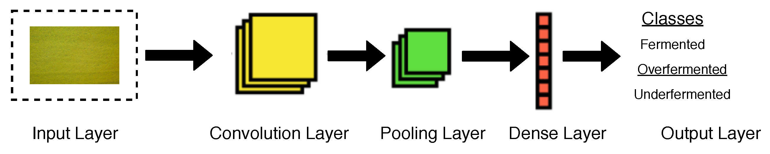
Convolutional Neural Network (CNN) is a class of deep learning technique that is currently emerging in solving computer vision challenges, which includes detection of objects [91], segmentation [92], and dimage classification [93], among others. CNN emerged in the mid-2000s due to the development in computing power of hardware of the computer [94]. A CNN is composed of the following layers (Figure 11): an input layer, convolutional layer, pooling layer, dense layer, and output layer. An input layer of a CNN is the layer where the input is passed to the network. In Figure 11, the input layer contains an image which needs to be classified [95]. Convolutional layers are a set of filters needed to learn. The filters are used to calculate output feature maps, with all units in a feature map sharing the same weights [96,97,98]. A pooling layer will then sum up the activities and selects the maximum values in the neighborhood of each feature map [99]. A dense layer consists of neurons in a neural network which receive inputs from all the neurons in the previous layer [100]. Convolutional has shown high accuracy in image recognition tasks; however, they have high computation tasks [101].
3.4.5. Support Vector Machine (SVM)
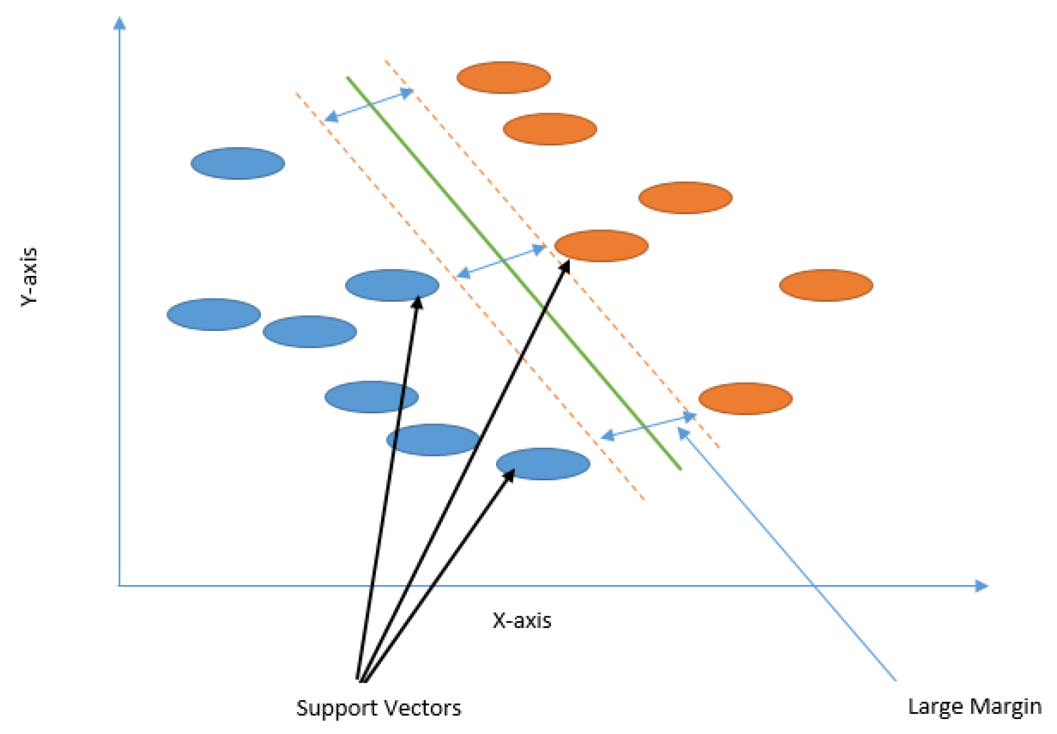
Support Vector Machine (SVM) is a non-probabilistic binary classifier that aims at finding a hyperplane with a maximum margin to separate high dimension classes by focusing on the training samples located at the edge of the class distribution [102]. The model is based on statistical learning theory and the structural risk minimization theory [103]. The model chooses extreme vectors which help in creating the hyperplane. These extreme points are referred to as support vectors. The binary classification problem with linear separability (Figure 12) has a goal to find the optimum hyperplane, through maximizing the margin and through minimizing the classification error between each class.
3.4.6. Naive Bayes (NB)
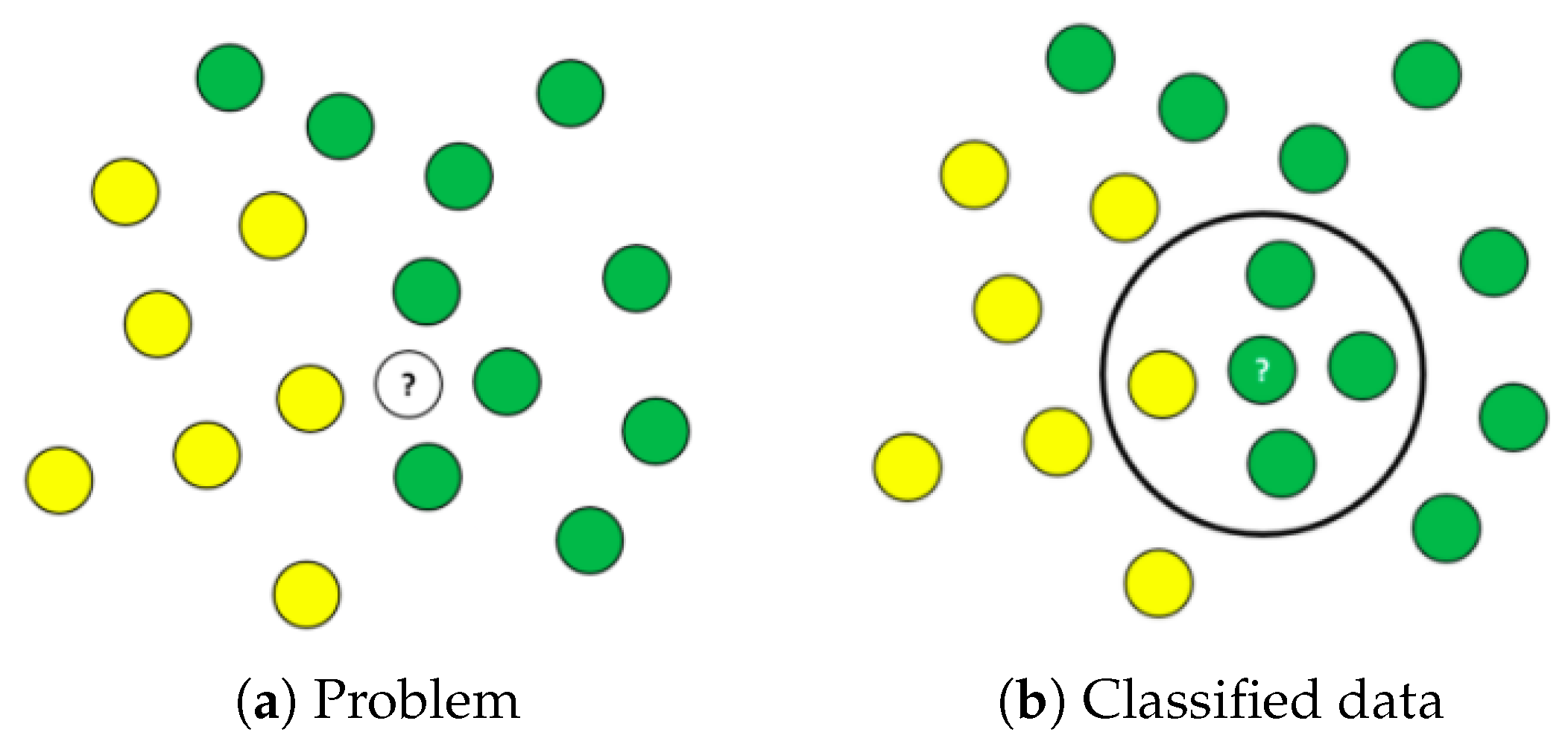
Naive Bayes is a probabilistic model based on Bayes’ theorem. Bayes’ theorem provides the relationship between the probabilities of two events and their conditional probabilities [108,109,110]. A Naive Bayes classifier assumes that the presence or absence of a particular feature of a class is unrelated to the presence or absence of other features [111,112]. In classification tasks, NB constructs a probabilistic model of the features and applies the model in prediction of the new instances. Figure 13 shows a sample of balls belonging to two classes: yellow and green. The task is to estimate the class for which the ball with a question mark belongs to. There is a very high probability that the ball belongs to class green since most of the balls belong to that class.
3.4.7. Linear Discriminant Analysis (LDA)
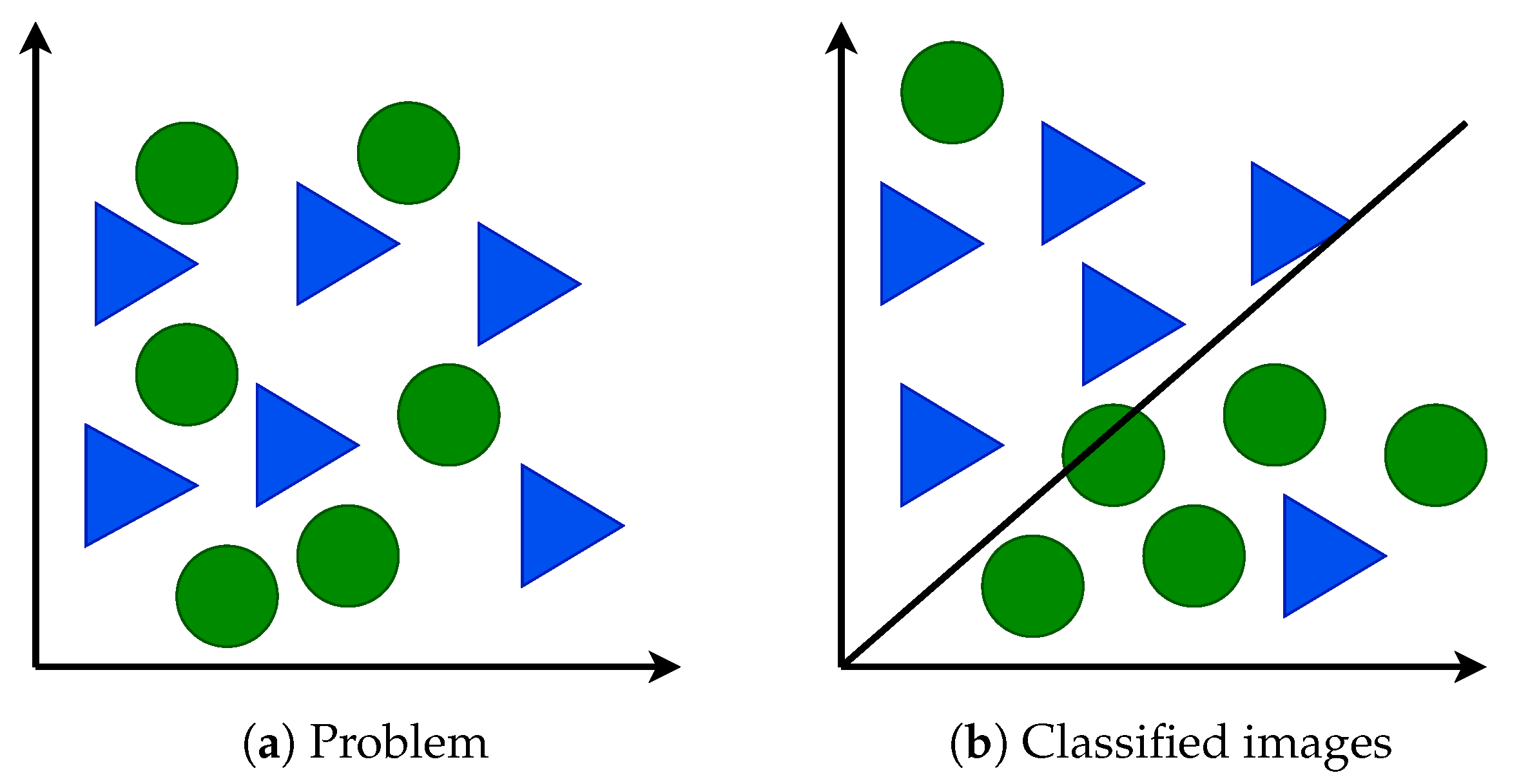
Linear discriminant analysis is an approach developed by the famous statistician R.A. Fisher, who arrived at linear discriminants from a different perspective [113]. He was interested in finding a linear projection for data that maximizes the variance between classes relative to the variance for data from the same class [114]. LDA combines features of a class and builds on separating the classes. It models the differences between classes and builds a vector for differentiating the classes based on the difference in the classes [115,116]. LDA is popular because of its low-cost implementation and its ease of adaptation for discriminating nonlinearly separable classes through the kernel trick method [117], among others. Some of the weaknesses of LDA includes its challenge in handling large datasets, among others [118]. Figure 14a shows a classification problem, while Figure 14b shows the solution to the classification problem using LDA.
3.5. TeaNet
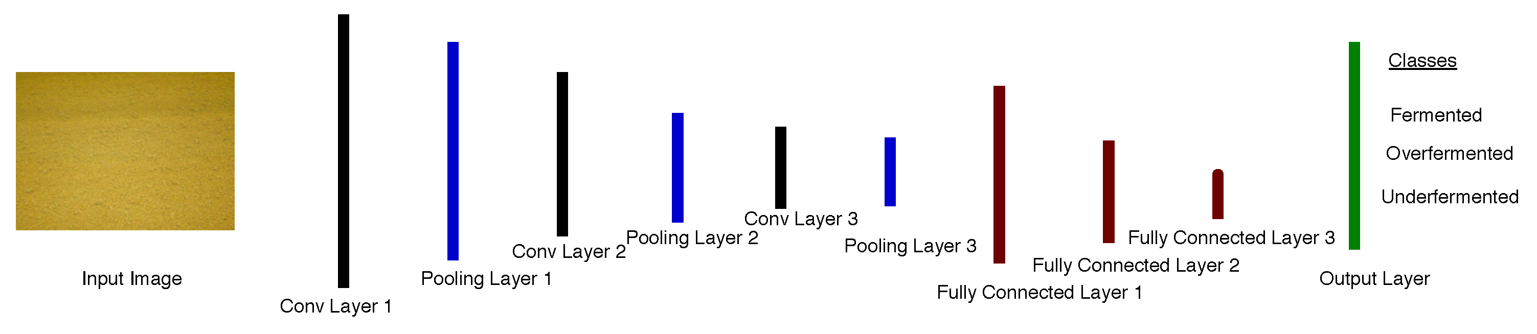
TeaNet is a deep learning model based on Convolutional Neural Network (CNN). The network architecture of TeaNet is an improvement upon the standard AlexNet model [119]. We designed an optimum tea fermentation detection model with relatively simple network structure and small computational needs. To construct TeaNet, we reduced the number of convolutional layer filters and the number of nodes in the fully connected layer. This reduces the number of parameters that require training, thus reducing the overfitting problem. The basic architecture of the network is shown in Figure 15.
The input images were rescaled to 150 × 150 pixels, and the three color channels discussed in Section 3.3.1 were all processed directly by the network. Table 4 shows the layer parameters of TeaNet.
The layers are defined as follows:
- The first convolutional layer comprises of 32 filters and a kernel size of 11 × 11 pixels. This layer is followed by a rectified linear unit (ReLU) operation. ReLU is an activation function that provides a solution to vanishing gradients [96]. Its pooling layer has a kernel size of 3 ×3 pixels, with two strides.
- The second convolutional layer comprises of 64 filters and a kernel size of 3 × 3 pixels and is followed by a ReLU operation; its pooling layer has a kernel size of 2 × 2 pixels.
- Additionally, the third convolutional layer comprises of 128 filters and a kernel size of 3 × 3 pixels, followed by ReLU with a kernel size of 2 × 2 pixels.
- The first full connection layer was made up of 512 neurons, followed by a ReLu and a dropout operation. The dropout operation [120] is proposed to solve overfitting as it trains only a randomly selected nodes. We set the ratio of dropout to 0.5.
- The second full convolutional layer had 128 neurons and was followed by a ReLU and dropout operations.
- The last fully convolutional layer contains three neurons, which represent 3 classes of images in tea fermentation and LabelMe datasets. The output of this layer is transferred to the output layer to determine the class of the input image. A softmax activation function is then implemented to force the sum of the output values to be equal to 1.0. Softmax also limits the individual output values between 0–1.
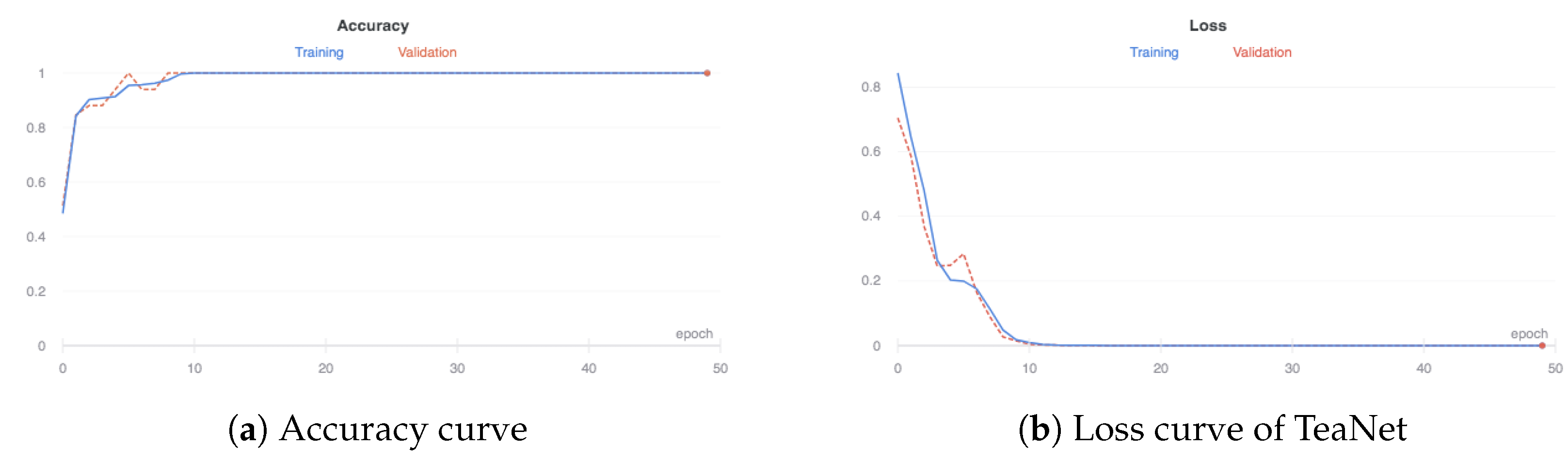
At the beginning, the weights of the layers were initialized with random values from a Gaussian distribution. To train the network, a stochastic gradient descent (SGD) technique with a batch size of 16 and a momentum value of 0.9 [121] was adopted. Initially, the learning rate across the network was set to 0.1, and a minumum threshold was set at 0.0001. The number of epochs was set as 50, and the weight decay was set to 0.0005. The accuracy of TeaNet increased with an increase in epoch, and it achieved an accuracy of 1.0 at epoch 10 (Figure 16a). At the beginning of the iteration, the accuracy is low since the weights of the neurons are not fully set. After each iteration, the weights are updated. The validation accuracy shows a steady increase, and the model had an accuracy of 1.0. The loss of TeaNet during training and validation is illustrated in Figure 16b. There is a steady reduction in the loss from the first epoch up to epoch 10, where the loss value is at 0 for both the training and validation sets. From Figure 16, the model has good performance and is not overfitted as it records good results in unseen data.
4. Implementation
To implement the classification models discussed in Section 3.4 and the TeaNet model discussed in Section 3.5, python programming language was adopted. After implementation, it was necessary to evaluate the performance of the various classification models. This section provides the implementation of the models and the metrics that were adopted in evaluating their performances.
4.1. Implementation of the Classifiers
As mentioned in Section 4, we adopted python programming language to implement the classification models. Some of the reasons for adopting python were that it has rich libraries [122], that it has moderate learning curve [123], and that it is free and open source [124]. Some of the libraries that we adopted alongside python are Tensorflow [125,126], Keras [127], Seaborn [128], matplotlib [129], sklearn [130,131], OpenCV [56], pandas [132], and numpy [133]. The implemented classification models are available at http://classifier.sisiboportal.com/.
4.2. Evaluation Metrics
In Section 4, we mentioned the various evaluation metrics that were adopted in this study to evaluate the classification models. The following paragraphs discuss each of the metric in detail.
4.2.1. Precision
Precision is the ratio of the correct classification to the total number of classifications [134,135]. A low precision indicates a large number of false positives [136]. It can be represented by Equation (2).
where TP is an outcome where the model correctly classifies a class and FP is an outcome where the model incorrectly classifies a class.
4.2.2. Recall
Recall is the ratio of the number of correctly classified images to the total number of images [134,136]. It is the actual positives that are correctly classified to the correct classes. Recall can be represented by Equation (3).
where TP is an outcome where the model correctly classifies the positive class and FN is an outcome where the model incorrectly classifies the negative class.
4.2.3. F1-Score
4.2.4. Accuracy
Accuracy is the fraction of predictions that the model got right. Therefore, it is the sum of correct predictions divided by all the predictions. It can be represented by Equation (5).
where TP is an outcome where a model correctly classifies the positive class, FP is an outcome where a model incorrectly classifies the positive class, TN is an outcome where the model correctly classifies a negative class, and FN is an outcome where a model incorrectly classifies a negative class.
4.2.5. Logarithmic Loss
Logarithmic loss or log loss works by penalizing false classifications [134]. In classification tasks, it is the measure of the inaccuracy of classification. An ideal logarithmic loss should be 0. Logarithmic loss can be represented by Equation (6).
where g is the predicted probability and p is the true label.
4.2.6. Confusion Matrix
A confusion matrix is used to summarize the classification performance of a classifier with test data. Sensitivity in a confusion matrix measures the proportion of actual positives that are correctly identified and can be represented by Equation (7).
where TP is the number of correct classification while FN is an outcome where the model incorrectly classifies the negative class.
5. Evaluation Results
In this section, we provide the results of the evaluation of the classification models based on the metrics discussed in Section 4.2.
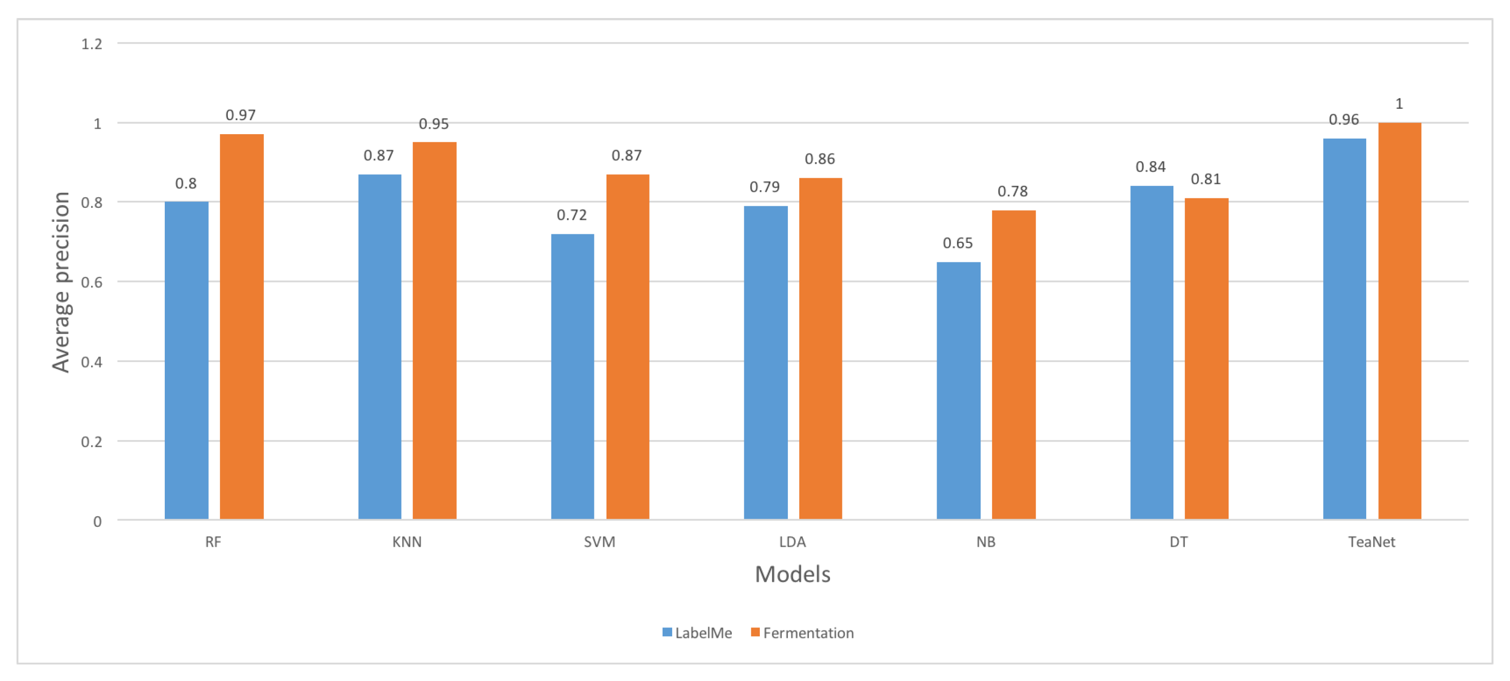
Results of the precision of the classifiers in the two datasets are shown in Figure 17. All the other classifiers generally categorized the majority of the images correctly. TeaNet classifier clearly performed better than the rest of the classifiers. TeaNet achieved average precisions of 1.0 and 0.96 in the tea fermentation and LabelMe datasets, respectively. Generally, the majority of the classifiers except decision tree produced better precision in the fermentation dataset compared to the LabelMe dataset. This is because there was a distinctive change in color in the 3 categories of fermentation images. The classifiers recorded an average precision of between 0.78–1.00 in the fermentation dataset and between 0.65–0.96 for the LabelMe dataset.
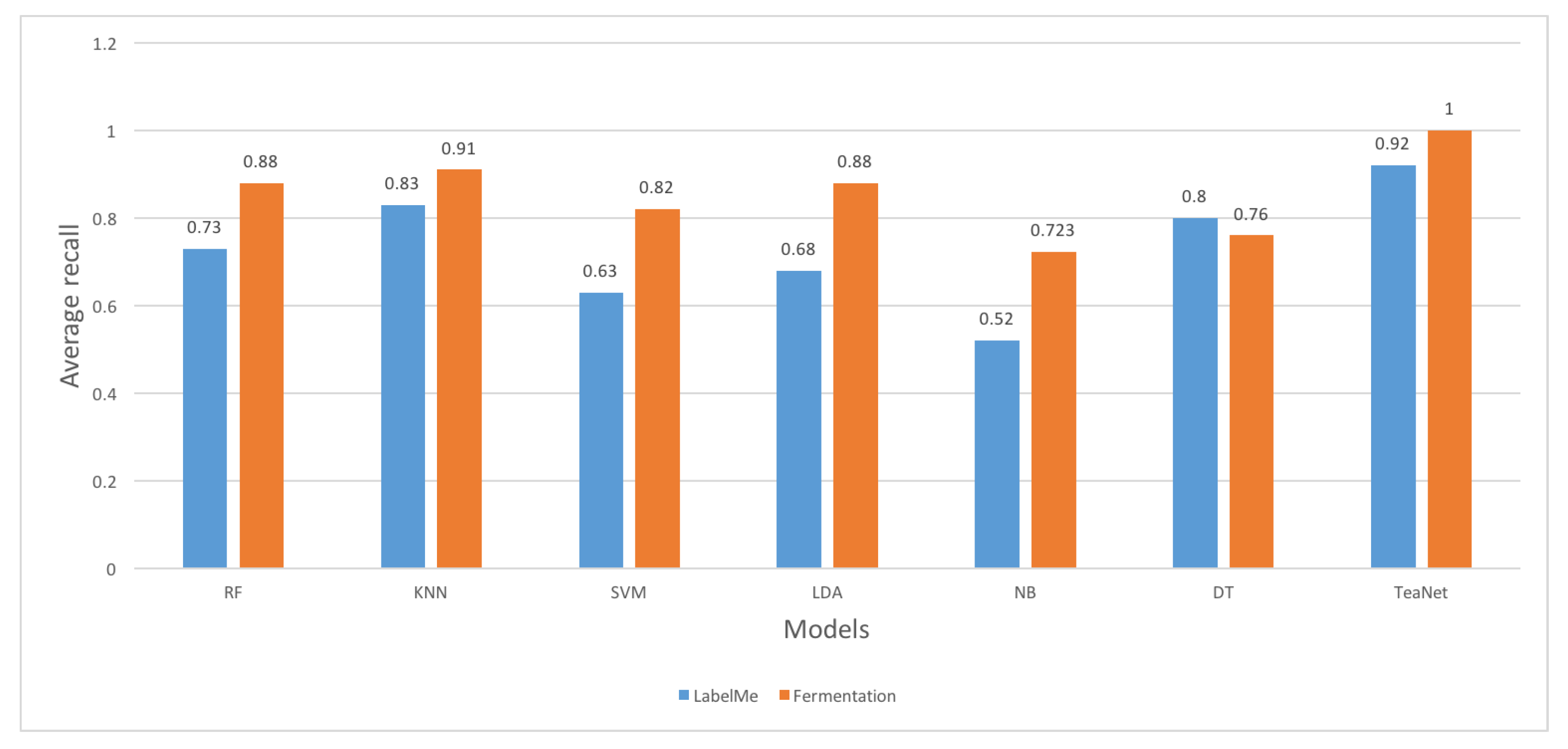
Recall values are illustrated in Figure 18. Once again, TeaNet outperformed the other classifiers by producing the highest average recall values across the datasets. The majority of the classifiers had better performances in the tea fermentation dataset compared to the LabelMe dataset. The classifiers had an average recall of 0.75–1.0 for the tea fermentation dataset and an average of 0.58–0.96 for LabelMe dataset. KNN also had a good performance by recording average recalls of 0.93 and 0.85 for the tea fermentation and the LabelMe dataset, respectively. Naive Bayes recorded the lowest recall values. From these results, it is evident that TeaNet and KNN produced the best recall values.
We compared the F1 score of TeaNet with the other classifiers and presented the results in Figure 19. The F1 score values of TeaNet was higher than the other classifiers. The classifiers recorded F1 values of between 0.58–0.9 for the LabelMe dataset and between 0.75–1.00 for the tea fermentation dataset. We can note that TeaNet showed alot of effectiveness as it achieved an F1 of 1.00 in the tea Fermentation dataset and of 0.9 for the LabelMe dataset (Figure 19). KNN also recorded good performances of 0.93 and 0.85 for tea fermentation and LabelMe datasets, respectively.
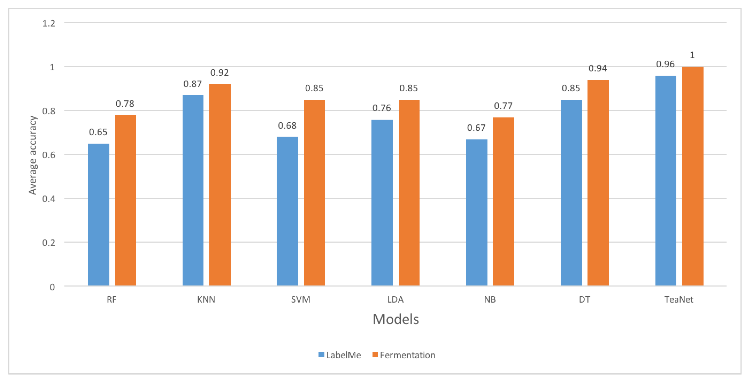
The performance of the classifiers in terms of accuracy is presented in Figure 20. The majority of the classifiers had good accuracy results. TeaNet achieved an average accuracy of 1.00 for the tea fermentation dataset and an average accuracy of 0.958 for the LabelMe dataset. This shows that TeaNet once again outperforms the other classifiers. Each of the classifiers produced an accuracy of more than 0.6 across the datasets. It shows that the probability of each of the classifiers in classifying the dataset is more than 60%. Naive Bayes recorded average accuracies of 0.67 and 0.77 for the LabelMe and tea fermentation dataset, respectively. On the other hand, decision tree recorded average accuracies of 0.94 and 0.85 for the tea fermentation and the LabelMe datasets, respectively. These results show that the majority of the classifiers can be applied to detect the tea fermentation images.
Additionally, logarithmic losses of the classifiers were evaluated. The results of the analysis are shown in Figure 21. TeaNet had the least logarithmic loss at 0.136 and 0.09 for LabelMe and Fermentation dataset, respectively (Figure 21). Generally, the Logarithmic losses recorded by the majority of the models was higher than 0.55 for the LabelMe dataset. For tea fermentation, the majority of the models had logarithmic loss of less than 0.50. Evidently, most of the classifiers had a lower logarithmic loss in the fermentation dataset compared to the LabelMe dataset. Random forest recorded the highest logarithmic loss at 0.7 for the LabelMe dataset. On the other hand, Naive Bayes recorded the highest logarithmic loss of 0.64 for the tea fermentation dataset.
Finally, a confusion matrix was used to further evaluate the classification models and results are shown in Table 5. The least specificity recorded by the classifiers was 73.5%, and the highest was 100.0%. TeaNet recorded an average sensitivity of 100% for fermented, an average of 100% for overfermented, and finally an average of 100% for underfermented. TeaNet outperformed the other classifiers. Consequently, the TeaNet proposed to classify tea images is superior to the other previously described algorithms.
6. Conclusions and Future Work
In this paper, we have proposed a deep learning model dubbed TeaNet. We have assessed the capabilities of TeaNet and other standard machine learning classifiers in categorizing images. We used tea fermentation and LabelMe datasets for training and evaluating the classifiers. From the experimental results, TeaNet outperformed the other classifiers in the classification tasks. In general, all the classifiers had good performance across the two datasets. These results show that the majority of the classifiers can be used in real deployments. Importantly, the effectiveness of TeaNet in the tea fermentation dataset is a great achievement. This is a game changer in the application of deep learning in agriculture and most specifically in tea fermentation.
Additionally, the results from this study highlight the feasibility of applying TeaNet in the detection of tea fermentation, which would significantly improve the process. This will, in turn, increase the quality of produced tea and subsequently increase the value of the made tea. This will lead to improved livelihoods of the farmers and to general improvement of the country’s GDP. The same technique can be applied to the fermentation of coffee and cocoa. In our future studies, we will implement TeaNet with the Internet of things in real deployment in a tea factory to monitor fermentation of black tea.
Author Contributions
Formal analysis, A.F.; methodology, G.K. and A.F.; software, G.K.; supervision, A.N., R.N.S., A.K., and A.F.; validation, G.K.; visualization, G.K.; writing—original draft, G.K.; writing—review and editing, A.N., R.N.S., A.K., and A.F. All authors have read and agreed to the published version of the manuscript.
Funding
This research was funded by African Center of Excellence in Internet of Things (ACEIoT) and Kenya Education Network (KENET) through the Computer Science, Information Systems, and Engineering multidisciplinary mini-grant.
Acknowledgments
G.K. wishes to thank A.F. for leading this research, for all the support in ensuring this work is a reality, and for the numerous advises and guidance throughout the research process. G.K. also wishes to put on record appreciation to R.N. and A.N. for their inputs in this work. Additionally, G.K. wishes to express appreciation to A.K. for all the mentorship, support, and guidance. Finally, the authors would like to express their appreciation to the anonymous reviewers and editors for their constructive comments.
Conflicts of Interest
The authors declare that there is no conflict of interest. The funders had no role in the design of the study; in the collection, analyses, or interpretation of data; in the writing of the manuscript; or in the decision to publish the results
Abbreviations
| ANN | Artificial Neural Network |
| CNN | Convolutional Neural Network |
| SVM | Support Vector Machine |
| DT | Decision Tree |
| RF | Random Forests |
| SVM | Support Vector Machine |
| KNN | K-Nearest Neighbor |
| OpenCV | Open Computer Vision |
| IoT | Internet of Things |
| TF | Theaflavins |
| TR | Thearubins |
| EN | electronic Nose |
| ET | electronic Tongue |
| LDA | Local Discriminant Analysis |
| NB | Naive Bayes |
| KTDA | Kenya Tea Development Agency |
| GDP | Gross Domestic Product |
| MSE | Mean Squarred Error |
| MAE | Mean Absolute Error |
References
- Sigley, G. Tea and China’s rise: Tea, nationalism and culture in the 21st century. Int. Commun. Chin. Cult. 2015, 2, 319–341. [Google Scholar] [CrossRef] [Green Version]
- Yiannakopoulou, E. Green Tea Catechins: Proposed Mechanisms of Action in Breast Cancer Focusing on the Interplay Between Survival and Apoptosis. Anti-Cancer Agents Med. Chem. 2014, 14, 290–295. [Google Scholar] [CrossRef]
- Miura, K.; Hughes, M.C.B.; Arovah, N.I.; Van Der Pols, J.C.; Green, A.C. Black Tea Consumption and Risk of Skin Cancer: An 11-Year Prospective Study. Nutr. Cancer 2015, 67, 1049–1055. [Google Scholar] [CrossRef] [PubMed]
- Hajiaghaalipour, F.; Kanthimathi, M.S.; Sanusi, J.; Rajarajeswaran, J. White tea (Camellia sinensis) inhibits proliferation of the colon cancer cell line, HT-29, activates caspases and protects DNA of normal cells against oxidative damage. Food Chem. 2015, 169, 401–410. [Google Scholar] [CrossRef] [PubMed] [Green Version]
- Sironi, E.; Colombo, L.; Lompo, A.; Messa, M.; Bonanomi, M.; Regonesi, M.E.; Salmona, M.; Airoldi, C. Natural compounds against neurodegenerative diseases: Molecular characterization of the interaction of catechins from green tea with Aβ1-42, PrP106-126, and ataxin-3 oligomers. Chem. A Eur. J. 2014, 20, 13793–13800. [Google Scholar] [CrossRef] [PubMed]
- Gopalakrishna, R.; Fan, T.; Deng, R.; Rayudu, D.; Chen, Z.W.; Tzeng, W.S.; Gundimeda, U. Extracellular matrix components influence prostate tumor cell sensitivity to cancer-preventive agents selenium and green tea polyphenols. In Proceedings of the AACR Annual Meeting 2014, San Diego, CA, USA, 5–9 April 2014; American Association for Cancer Research (AACR): Philadelphia, PA, USA, 2014; p. 232. [Google Scholar] [CrossRef]
- Lazaro, J.B.; Ballado, A.; Bautista, F.P.F.; So, J.K.B.; Villegas, J.M.J. Chemometric data analysis for black tea fermentation using principal component analysis. In AIP Conference Proceedings; AIP Publishing LLC: Melville, NY, USA, 2018; Volume 2045, p. 020050. [Google Scholar] [CrossRef]
- Saikia, D.; Boruah, P.K.; Sarma, U. A Sensor Network to Monitor Process Parameters of Fermentation and Drying in Black Tea Production. MAPAN 2015, 30, 211–219. [Google Scholar] [CrossRef]
- Mitei, Z. Growing sustainable tea on Kenyan smallholder farms. Int. J. Agric. Sustain. 2011, 9, 59–66. [Google Scholar] [CrossRef] [Green Version]
- Kamunya, S.M.; Wachira, F.N.; Pathak, R.S.; Muoki, R.C.; Sharma, R.K. Tea Improvement in Kenya. In Advanced Topics in Science and Technology in China; Springer: Berlin/Heidelberg, Germany, 2012; pp. 177–226. [Google Scholar] [CrossRef]
- Kagira, E.K.; Kimani, S.W.; Githii, K.S. Sustainable Methods of Addressing Challenges Facing Small Holder Tea Sector in Kenya: A Supply Chain Management Approach. J. Manag. Sustain. 2012, 2. [Google Scholar] [CrossRef] [Green Version]
- Tea Board of Kenya. Kenya Tea Yearly Report; Technical Report; Tea Board of Kenya: Nairobi, Kenya, 2018. [Google Scholar]
- Onduru, D.D.; De Jager, A.; Hiller, S.; Van Den Bosch, R. Sustainability of Smallholder Tea Production in Developing Countries: Learning Experiences from Farmer Field Schools in Kenya; International Journal of Development and Sustainability: Tokyo, Japan, 2012. [Google Scholar]
- Xu, M.; Wang, J.; Gu, S. Rapid identification of tea quality by E-nose and computer vision combining with a synergetic data fusion strategy. J. Food Eng. 2019, 241, 10–17. [Google Scholar] [CrossRef]
- Jayabalan, R.; Malbaša, R.V.; Lončar, E.S.; Vitas, J.S.; Sathishkumar, M. A Review on Kombucha Tea-Microbiology, Composition, Fermentation, Beneficial Effects, Toxicity, and Tea Fungus. Compr. Rev. Food Sci. Food Saf. 2014, 13, 538–550. [Google Scholar] [CrossRef]
- Jolvis Pou, K. Fermentation: The Key Step in the Processing of Black Tea. J. Biosyst. Eng. 2016, 41, 85–92. [Google Scholar] [CrossRef] [Green Version]
- Asil, M.H.; Rabiei, B.; Ansari, R. Optimal fermentation time and temperature to improve biochemical composition and sensory characteristics of black tea. Aust. J. Crop. Sci. 2012, 6, 550–558. [Google Scholar]
- Memisevic, R. Deep learning: Architectures, algorithms, applications. In Proceedings of the 2015 IEEE Hot Chips 27 Symposium, HCS 2015, Cupertino, CA, USA, 22–25 August 2015. [Google Scholar] [CrossRef]
- Luckow, A.; Kennedy, K.; Ziolkowski, M.; Djerekarov, E.; Cook, M.; Duffy, E.; Schleiss, M.; Vorster, B.; Weill, E.; Kulshrestha, A.; et al. Artificial Intelligence and Deep Learning Applications for Automotive Manufacturing. In Proceedings of the 2018 IEEE International Conference on Big Data (Big Data 2018), Seattle, WA, USA, 10–13 December 2018; pp. 3144–3152. [Google Scholar] [CrossRef]
- Shinde, P.P.; Shah, S. A Review of Machine Learning and Deep Learning Applications. In Proceedings of the 2018 4th International Conference on Computing, Communication Control and Automation (ICCUBEA 2018), Pune, India, 16–18 August 2018. [Google Scholar] [CrossRef]
- Zhu, W.; Xie, L.; Han, J.; Guo, X. The Application of Deep Learning in Cancer Prognosis Prediction. Cancers 2020, 12, 603. [Google Scholar] [CrossRef] [PubMed] [Green Version]
- Khan, S.; Yairi, T. A review on the application of deep learning in system health management. Mech. Syst. Signal Process. 2018. [Google Scholar] [CrossRef]
- Pouyanfar, S.; Sadiq, S.; Yan, Y.; Tian, H.; Tao, Y.; Reyes, M.P.; Shyu, M.L.; Chen, S.C.; Iyengar, S.S. A survey on deep learning: Algorithms, techniques, and applications. ACM Comput. Surv. (CSUR) 2018. [Google Scholar] [CrossRef]
- Dargan, S.; Kumar, M.; Ayyagari, M.R.; Kumar, G. A Survey of Deep Learning and Its Applications: A New Paradigm to Machine Learning. Arch. Comput. Methods Eng. 2019, 1–22. [Google Scholar] [CrossRef]
- Mahmud, M.; Kaiser, M.S.; Hussain, A.; Vassanelli, S. Applications of Deep Learning and Reinforcement Learning to Biological Data. IEEE Trans. Neural Netw. Learn. Syst. 2018, 29, 2063–2079. [Google Scholar] [CrossRef] [Green Version]
- Gibson, K.; Förster, A. Black Tea Fermentation Dataset; Technical Report; Mendeley Ltd.: London, UK, 2020. [Google Scholar] [CrossRef]
- Barcelo-Ordinas, J.M.; Chanet, J.P.; Hou, K.M.; García-Vidal, J. A Survey of Wireless Sensor Technologies Applied to Precision Agriculture; Wageningen Academic Publishers: Wageningen, The Netherlands, 2013; pp. 801–808. [Google Scholar]
- Ghosh, S.; Tudu, B.; Bhattacharyya, N.; Bandyopadhyay, R. A recurrent Elman network in conjunction with an electronic nose for fast prediction of optimum fermentation time of black tea. Neural Comput. Appl. 2019, 31, 1165–1171. [Google Scholar] [CrossRef]
- Bhattacharyya, N.; Seth, S.; Tudu, B.; Tamuly, P.; Jana, A.; Ghosh, D.; Bandyopadhyay, R.; Bhuyan, M. Monitoring of black tea fermentation process using electronic nose. J. Food Eng. 2007, 80, 1146–1156. [Google Scholar] [CrossRef]
- Mohit Sharma, D.G.; Nabarun Bhattacharya. Electronic Nose—A new way for predicting the optimum point of fermentation of Black Tea. Int. J. Eng. Sci. Invent. 2012, 12, 56–60. [Google Scholar]
- Manigandan, N. Handheld Electronic Nose (HEN) for detection of optimum fermentation time during tea manufacture and assessment of tea quality. Int. J. Adv. Res. 2019, 7, 697–702. [Google Scholar] [CrossRef] [Green Version]
- Das, A.; Ghosh, T.K.; Ghosh, A.; Ray, H. An embedded Electronic Nose for identification of aroma index for different tea aroma chemicals. In Proceedings of the International Conference on Sensing Technology (ICST 2012), Kolkata, India, 18–21 December 2012; pp. 577–582. [Google Scholar] [CrossRef]
- Ai, S.; Wu, R.; Yan, L.; Wu, Y. Evaluation of taste quality in green tea infusion using electronic tongue combined with LS-SVM. In Advanced Materials Research; Trans Tech Publications Ltd.: Stäfa, Switzerland, 2011; Volume 301–303, pp. 1643–1647. [Google Scholar] [CrossRef]
- Zhong, Y.H.; Zhang, S.; He, R.; Zhang, J.; Zhou, Z.; Cheng, X.; Huang, G.; Zhang, J. A Convolutional Neural Network Based Auto Features Extraction Method for Tea Classification with Electronic Tongue. Appl. Sci. 2019, 9, 2518. [Google Scholar] [CrossRef] [Green Version]
- Lvova, L. Electronic Tongue Principles and Applications in the Food Industry. In Electronic Noses and Tongues in Food Science; Elsevier Inc.: Amsterdam, The Netherlands, 2016; pp. 151–160. [Google Scholar] [CrossRef]
- Li, H.; Zhang, B.; Hu, W.; Liu, Y.; Dong, C.; Chen, Q. Monitoring black tea fermentation using a colorimetric sensor array-based artificial olfaction system. J. Food Process. Preserv. 2018, 42, e13348. [Google Scholar] [CrossRef] [Green Version]
- Ghosh, A.; Sharma, P.; Tudu, B.; Sabhapondit, S.; Baruah, B.D.; Tamuly, P.; Bhattacharyya, N.; Bandyopadhyay, R. Detection of Optimum Fermentation Time of Black CTC Tea Using a Voltammetric Electronic Tongue. IEEE Trans. Instrum. Meas. 2015, 64, 2720–2729. [Google Scholar] [CrossRef]
- Zhi, R.; Zhao, L.; Zhang, D. A framework for the multi-level fusion of electronic nose and electronic tongue for tea quality assessment. Sensors 2017, 17, 1007. [Google Scholar] [CrossRef] [Green Version]
- Akuli, A.; Pal, A.; Dey, T.; Bej, G.; Santra, A.; Majumdar, S.; Bhattacharyya, N. Assessment of Black Tea Using Low-Level Image Feature Extraction Technique. In Proceedings of the Global AI Congress 2019; Springer: Singapore, 2020; pp. 453–467. [Google Scholar] [CrossRef]
- Dong, C.; Liang, G.; Hu, B.; Yuan, H.; Jiang, Y.; Zhu, H.; Qi, J. Prediction of Congou Black Tea Fermentation Quality Indices from Color Features Using Non-Linear Regression Methods. Sci. Rep. 2018, 8, 10535. [Google Scholar] [CrossRef] [Green Version]
- Binh, P.T.; Du, D.H.; Nhung, T.C. Control and Optimize Black Tea Fermentation Using Computer Vision and Optimal Control Algorithm. In Lecture Notes in Networks and Systems; Springer: Berlin/Heidelberg, Germany, 2020; Volume 104, pp. 310–319. [Google Scholar] [CrossRef]
- Saranka, S.; Thangathurai, K.; Wanniarachchi, C.; Wanniarachchi, W.K. Monitoring Fermentation of Black Tea with Image Processing Techniques. IPSL 2016, 32, 31–37. [Google Scholar]
- Kumar, A.; Singh, H.; Sharma, S.; Kumar, A. Color Analysis of Black Tea Liquor Using Image Processing Techniques. IJECT 2011, 2, 292–296. [Google Scholar]
- Ghosh, A.; Bag, A.K.; Sharma, P.; Tudu, B.; Sabhapondit, S.; Baruah, B.D.; Tamuly, P.; Bhattacharyya, N.; Bandyopadhyay, R. Monitoring the fermentation process and detection of optimum fermentation time of black tea using an electronic tongue. IEEE Sens. J. 2015, 15, 6255–6262. [Google Scholar] [CrossRef]
- Kim, Y.; Chung, M. An Approach to Hyperparameter Optimization for the Objective Function in Machine Learning. Electronics 2019, 8, 1267. [Google Scholar] [CrossRef] [Green Version]
- Li, J.; Wang, J.Z. Automatic linguistic indexing of pictures by a statistical modeling approach. IEEE Trans. Pattern Anal. Mach. Intell. 2003, 25, 1075–1088. [Google Scholar] [CrossRef] [Green Version]
- Tylecek, R.; Fisher, R. Consistent Semantic Annotation of Outdoor Datasets via 2D/3D Label Transfer. Sensors 2018, 18, 2249. [Google Scholar] [CrossRef] [PubMed] [Green Version]
- Fabijańska, A.; Sankowski, D. Image noise removal—The new approach. In Proceedings of the 2007 9th International Conference—The Experience of Designing and Applications of CAD Systems in Microelectronics, Lviv-Polyana, Ukraine, 19–24 February 2007; pp. 457–459. [Google Scholar] [CrossRef]
- Ahmad, K.; Khan, J.; Iqbal, M.S.U.D. A comparative study of different denoising techniques in digital image processing. In Proceedings of the 2019 8th International Conference on Modeling Simulation and Applied Optimization (ICMSAO 2019), Zallaq, Bahrain, 15–17 April 2019. [Google Scholar] [CrossRef]
- Mistry, Y.; Ingole, D.T.; Ingole, M.D. Content based image retrieval using hybrid features and various distance metric. J. Electr. Syst. Inf. Technol. 2017. [Google Scholar] [CrossRef]
- Yang, Y.G.; Zou, L.; Zhou, Y.H.; Shi, W.M. Visually meaningful encryption for color images by using Qi hyper-chaotic system and singular value decomposition in YCbCr color space. Optik 2020, 164422. [Google Scholar] [CrossRef]
- Alamgir, N.; Nguyen, K.; Chandran, V.; Boles, W. Combining multi-channel color space with local binary co-occurrence feature descriptors for accurate smoke detection from surveillance videos. Fire Saf. J. 2018, 102, 1–10. [Google Scholar] [CrossRef] [Green Version]
- Li, Z.H.; Han, D.; Yang, C.J.; Zhang, T.Y.; Yu, H.Q. Probing operational conditions of mixing and oxygen deficiency using HSV color space. J. Environ. Manag. 2019, 232, 985–992. [Google Scholar] [CrossRef]
- Garcia-Lamont, F.; Cervantes, J.; López, A.; Rodriguez, L. Segmentation of images by color features: A survey. Neurocomputing 2018, 292, 1–27. [Google Scholar] [CrossRef]
- Novak, C.L.; Shafer, S.A. Anatomy of a color histogram. In Proceedings of the IEEE Computer Society Conference on Computer Vision and Pattern Recognition, Champaign, IL, USA, 15–18 June 1992; Volume 1992-June, pp. 599–605. [Google Scholar] [CrossRef] [Green Version]
- Jung, H.; Koo, K.; Yang, H. Measurement-Based Power Optimization Technique for OpenCV on Heterogeneous Multicore Processor. Symmetry 2019, 11, 1488. [Google Scholar] [CrossRef] [Green Version]
- Saroja, G.A.S.; Sulochana, C.H. Texture analysis of non-uniform images using GLCM. In Proceedings of the 2013 IEEE Conference on Information and Communication Technologies (ICT 2013), Thuckalay, India, 11–12 April 2013; pp. 1319–1322. [Google Scholar] [CrossRef]
- Kumar, G.; Bhatia, P.K. A detailed review of feature extraction in image processing systems. In Proceedings of the International Conference on Advanced Computing and Communication Technologies (ACCT), Rohtak, India, 8–9 February 2014; pp. 5–12. [Google Scholar] [CrossRef]
- Preethi, G.; Sornagopal, V. MRI image classification using GLCM texture features. In Proceedings of the IEEE International Conference on Green Computing, Communication and Electrical Engineering (ICGCCEE 2014), Coimbatore, India, 6–8 March 2014. [Google Scholar] [CrossRef]
- Akanbi, O.A.; Amiri, I.S.; Fazeldehkordi, E.; Akanbi, O.A.; Amiri, I.S.; Fazeldehkordi, E. Chapter 4—Feature Extraction. In A Machine-Learning Approach to Phishing Detection and Defense; Syngress: Rockland, MA, USA, 2015; pp. 45–54. [Google Scholar] [CrossRef]
- Xiaofeng, F.; Wei, W. Centralized binary patterns embedded with image euclidean distance for facial expression recognition. In Proceedings of the 4th International Conference on Natural Computation (ICNC 2008), Jinan, China, 18–20 October 2008; Volume 4, pp. 115–119. [Google Scholar] [CrossRef]
- Saravanan, C. Color image to grayscale image conversion. In Proceedings of the 2010 2nd International Conference on Computer Engineering and Applications (ICCEA 2010), Bali Island, Indonesia, 19–21 March 2010; Volume 2, pp. 196–199. [Google Scholar] [CrossRef]
- EMC Education Services. Data Science & Big Data Analytics; John Wiley & Sons, Inc.: Indianapolis, IN, USA, 2015. [Google Scholar] [CrossRef]
- Dahan, H.; Cohen, S.; Rokach, L.; Maimon, O. Proactive Data Mining with Decision Trees; SpringerBriefs in Electrical and Computer Engineering; Springer: New York, NY, USA, 2014. [Google Scholar] [CrossRef]
- Navada, A.; Ansari, A.N.; Patil, S.; Sonkamble, B.A. Overview of use of decision tree algorithms in machine learning. In Proceedings of the 2011 IEEE Control and System Graduate Research Colloquium (ICSGRC 2011), Shah Alam, Malaysia, 27–28 June 2011; pp. 37–42. [Google Scholar] [CrossRef]
- Brunello, A.; Marzano, E.; Montanari, A.; Sciavicco, G. J48SS: A novel decision tree approach for the handling of sequential and time series data. Computers 2019, 8, 21. [Google Scholar] [CrossRef] [Green Version]
- Park, S.; Hamm, S.Y.; Kim, J. Performance Evaluation of the GIS-Based Data-Mining Techniques Decision Tree, Random Forest, and Rotation Forest for Landslide Susceptibility Modeling. Sustainability 2019, 11, 5659. [Google Scholar] [CrossRef] [Green Version]
- Alajali, W.; Zhou, W.; Wen, S.; Wang, Y. Intersection Traffic Prediction Using Decision Tree Models. Symmetry 2018, 10, 386. [Google Scholar] [CrossRef] [Green Version]
- Han, J.; Fang, M.; Ye, S.; Chen, C.; Wan, Q.; Qian, X. Using Decision Tree to Predict Response Rates of Consumer Satisfaction, Attitude, and Loyalty Surveys. Sustainability 2019, 11, 2306. [Google Scholar] [CrossRef] [Green Version]
- Al Hamad, M.; Zeki, A.M. Accuracy vs. cost in decision trees: A survey. In Proceedings of the 2018 International Conference on Innovation and Intelligence for Informatics, Computing, and Technologies (3ICT 2018), Sakhier, Bahrain, 18–20 November 2018. [Google Scholar] [CrossRef]
- Feng, D.; Deng, Z.; Wang, T.; Liu, Y.; Xu, L. Identification of disturbance sources based on random forest model. In Proceedings of the 2018 International Conference on Power System Technology (POWERCON 2018), Guangzhou, China, 6–8 November 2018; pp. 3370–3375. [Google Scholar] [CrossRef]
- Samarakoon, P.N.; Promayon, E.; Fouard, C. Light Random Regression Forests for automatic multi-organ localization in CT images. In Proceedings of the International Symposium on Biomedical Imaging, Melbourne, Australia, 18–21 April 2017; pp. 371–374. [Google Scholar] [CrossRef] [Green Version]
- Georganos, S.; Grippa, T.; Gadiaga, A.; Vanhuysse, S.; Kalogirou, S.; Lennert, M.; Linard, C. An application of geographical random forests for population estimation in Dakar, Senegal using very-high-resolution satellite imagery. In Proceedings of the 2019 Joint Urban Remote Sensing Event (JURSE 2019), Vannes, France, 22–24 May 2019. [Google Scholar] [CrossRef]
- Liu, Y.; Liu, L.; Gao, Y.; Yang, L. An improved random forest algorithm based on attribute compatibility. In Proceedings of the 2019 IEEE 3rd Information Technology, Networking, Electronic and Automation Control Conference (ITNEC 2019), Chengdu, China, 15–17 March 2019; pp. 2558–2561. [Google Scholar] [CrossRef]
- Saffari, A.; Leistner, C.; Santner, J.; Godec, M.; Bischof, H. On-line random forests. In Proceedings of the IEEE 12th International Conference on Computer Vision Workshops (ICCV Workshops), Kyoto, Japan, 27 September–4 October 2009; pp. 1393–1400. [Google Scholar] [CrossRef]
- Kouzani, A.Z.; Nahavandi, S.; Khoshmanesh, K. Face classification by a random forest. In Proceedings of the TENCON 2007—2007 IEEE Region 10 Conference, Taipei, Taiwan, 30 October–2 November 2007. [Google Scholar] [CrossRef] [Green Version]
- More, A.S.; Rana, D.P. Review of random forest classification techniques to resolve data imbalance. In Proceedings of the 1st International Conference on Intelligent Systems and Information Management (ICISIM 2017), Aurangabad, India, 5–6 October 2017; Volume 2017-January, pp. 72–78. [Google Scholar] [CrossRef]
- Qunzhu, T.; Rui, Z.; Yufei, Y.; Chengyao, Z.; Zhijun, L. Improvement of random forest cascade regression algorithm and its application in fatigue detection. In Proceedings of the 2019 2nd International Conference on Electronics Technology (ICET 2019), Chengdu, China, 10–13 May 2019; pp. 499–503. [Google Scholar] [CrossRef]
- Patel, S.V.; Jokhakar, V.N. A random forest based machine learning approach for mild steel defect diagnosis. In Proceedings of the 2016 IEEE International Conference on Computational Intelligence and Computing Research (ICCIC 2016), Chennai, India, 15–17 December 2016. [Google Scholar] [CrossRef]
- Xu, B.; Ye, Y.; Nie, L. An improved random forest classifier for image classification. In Proceedings of the IEEE International Conference on Information and Automation (ICIA 2012), Shenyang, China, 6–8 June 2012; pp. 795–800. [Google Scholar] [CrossRef]
- Alam, M.S.; Vuong, S.T. Random forest classification for detecting android malware. In Proceedings of the 2013 IEEE International Conference on Green Computing and Communications and IEEE Internet of Things and IEEE Cyber, Physical and Social Computing, Beijing, China, 20–23 August 2013; pp. 663–669. [Google Scholar] [CrossRef]
- Thanh Noi, P.; Kappas, M. Comparison of Random Forest, k-Nearest Neighbor, and Support Vector Machine Classifiers for Land Cover Classification Using Sentinel-2 Imagery. Sensors 2017, 18, 18. [Google Scholar] [CrossRef] [Green Version]
- Saadatfar, H.; Khosravi, S.; Joloudari, J.H.; Mosavi, A.; Shamshirband, S. A New K-Nearest Neighbors Classifier for Big Data Based on Efficient Data Pruning. Mathematics 2020, 8, 286. [Google Scholar] [CrossRef] [Green Version]
- Florimbi, G.; Fabelo, H.; Torti, E.; Lazcano, R.; Madroñal, D.; Ortega, S.; Salvador, R.; Leporati, F.; Danese, G.; Báez-Quevedo, A.; et al. Accelerating the K-Nearest neighbors filtering algorithm to optimize the real-time classification of human brain tumor in hyperspectral images. Sensors 2018, 18, 2314. [Google Scholar] [CrossRef] [Green Version]
- Fan, G.F.; Guo, Y.H.; Zheng, J.M.; Hong, W.C. Application of the Weighted K-Nearest Neighbor Algorithm for Short-Term Load Forecasting. Energies 2019, 12, 916. [Google Scholar] [CrossRef] [Green Version]
- Aldayel, M.S. K-Nearest Neighbor classification for glass identification problem. In Proceedings of the International Conference on Computer Systems and Industrial Informatics (ICCSII), Sharjah, UAE, 18–20 December 2012. [Google Scholar] [CrossRef]
- Viswanath, P.; Hitendra Sarma, T. An improvement to k-nearest neighbor classifier. In Proceedings of the IEEE Recent Advances in Intelligent Computational Systems (RAICS), Trivandrum, India, 22–24 September 2011; pp. 227–231. [Google Scholar] [CrossRef] [Green Version]
- Sun, S.; Huang, R. An adaptive k-nearest neighbor algorithm. In Proceedings of the 2010 7th International Conference on Fuzzy Systems and Knowledge Discovery (FSKD), Yantai, China, 10–12 August 2010; Volume 1, pp. 91–94. [Google Scholar] [CrossRef]
- Zhang, S.; Li, X.; Zong, M.; Zhu, X.; Wang, R. Efficient kNN classification with different numbers of nearest neighbors. IEEE Trans. Neural Netw. Learn. Syst. 2018, 29, 1774–1785. [Google Scholar] [CrossRef]
- Jayaraman, P.P.; Zaslavsky, A.; Delsing, J. Intelligent processing of K-nearest neighbors queries using mobile data collectors in a location aware 3D wireless sensor network. In Lecture Notes in Computer Science (Including Subseries Lecture Notes in Artificial Intelligence and Lecture Notes in Bioinformatics); Springer: Berlin/Heidelberg, Germany, 2010; Volume 6098, pp. 260–270. [Google Scholar] [CrossRef]
- Cord, A.; Chambon, S. Automatic Road Defect Detection by Textural Pattern Recognition Based on AdaBoost. Comput.-Aided Civ. Infrastruct. Eng. 2012, 27, 244–259. [Google Scholar] [CrossRef]
- Roth, H.R.; Farag, A.; Lu, L.; Turkbey, E.B.; Summers, R.M. Deep convolutional networks for pancreas segmentation in CT imaging. Med. Imaging 2015 Image Process. 2015, 9413, 94131G. [Google Scholar] [CrossRef] [Green Version]
- Wang, W.; Wu, B.; Yang, S.; Wang, Z. Road Damage Detection and Classification with Faster R-CNN. In Proceedings of the 2018 IEEE International Conference on Big Data (Big Data 2018), Seattle, WA, USA, 10–13 December 2018; pp. 5220–5223. [Google Scholar] [CrossRef]
- Radopoulou, S.C.; Brilakis, I. Automated Detection of Multiple Pavement Defects. J. Comput. Civ. Eng. 2017, 31. [Google Scholar] [CrossRef] [Green Version]
- Chen, Q.; Fu, Y.; Song, W.; Cheng, K.; Lu, Z.; Zhang, C.; Li, L. An Efficient Streaming Accelerator for Low Bit-Width Convolutional Neural Networks. Electronics 2019, 8, 371. [Google Scholar] [CrossRef] [Green Version]
- Véstias, M.P. A Survey of Convolutional Neural Networks on Edge with Reconfigurable Computing. Algorithms 2019, 12, 154. [Google Scholar] [CrossRef] [Green Version]
- Chen, C.; Ma, Y.; Ren, G. A Convolutional Neural Network with Fletcher–Reeves Algorithm for Hyperspectral Image Classification. Remote Sens. 2019, 11, 1325. [Google Scholar] [CrossRef] [Green Version]
- Song, J.; Gao, S.; Zhu, Y.; Ma, C. A survey of remote sensing image classification based on CNNs. Big Earth Data 2019, 3, 232–254. [Google Scholar] [CrossRef]
- Cire\csan, D.C.; Meier, U.; Masci, J.; Gambardella, L.M.; Schmidhuber, J. Flexible, High Performance Convolutional Neural Networks for Image Classification. In Proceedings of the Twenty-Second International Joint Conference on Artificial Intelligence (IJCAI’11), Barcelona, Catalonia, Spain, 16–22 July 2011; Volume Two, pp. 1237–1242. [Google Scholar]
- Paoletti, M.; Haut, J.; Plaza, J.; Plaza, A. Deep&Dense Convolutional Neural Network for Hyperspectral Image Classification. Remote Sens. 2018, 10, 1454. [Google Scholar] [CrossRef] [Green Version]
- Hinton, G.; Deng, L.; Yu, D.; Dahl, G.; Mohamed, A.R.; Jaitly, N.; Senior, A.; Vanhoucke, V.; Nguyen, P.; Sainath, T.; et al. Deep neural networks for acoustic modeling in speech recognition: The shared views of four research groups. IEEE Signal Process. Mag. 2012, 29, 82–97. [Google Scholar] [CrossRef]
- Elaidi, H.; Elhaddar, Y.; Benabbou, Z.; Abbar, H. An idea of a clustering algorithm using support vector machines based on binary decision tree. In Proceedings of the 2018 International Conference on Intelligent Systems and Computer Vision (ISCV 2018), Fez, Morocco, 2–4 April 2018; Volume 2018-May, pp. 1–5. [Google Scholar] [CrossRef]
- Chao, C.F.; Horng, M.H. The construction of support vector machine classifier using the firefly algorithm. Comput. Intell. Neurosci. 2015, 2015. [Google Scholar] [CrossRef] [Green Version]
- Cheng, G.; Tong, X. Fuzzy clustering multiple kernel support vector machine. In Proceedings of the International Conference on Wavelet Analysis and Pattern Recognition, Chengdu, China, 15–18 July 2018; Volume 2018-July, pp. 7–12. [Google Scholar] [CrossRef]
- Shahbudin, S.; Zamri, M.; Kassim, M.; Abdullah, S.A.C.; Suliman, S.I. Weed classification using one class support vector machine. In Proceedings of the 2017 International Conference on Electrical, Electronics and System Engineering (ICEESE 2017), Kanazawa, Japan, 9–10 November 2017; Volume 2018-January, pp. 7–10. [Google Scholar] [CrossRef]
- Kranjčić, N.; Medak, D.; Župan, R.; Rezo, M. Support Vector Machine Accuracy Assessment for Extracting Green Urban Areas in Towns. Remote Sens. 2019, 11, 655. [Google Scholar] [CrossRef] [Green Version]
- Wang, D.; Peng, J.; Yu, Q.; Chen, Y.; Yu, H. Support Vector Machine Algorithm for Automatically Identifying Depositional Microfacies Using Well Logs. Sustainability 2019, 11, 1919. [Google Scholar] [CrossRef] [Green Version]
- Karthika, S.; Sairam, N. A Naïve Bayesian classifier for educational qualification. Indian J. Sci. Technol. 2015, 8. [Google Scholar] [CrossRef] [Green Version]
- Walia, H.; Rana, A.; Kansal, V. A Naïve Bayes Approach for working on Gurmukhi Word Sense Disambiguation. In Proceedings of the 2017 6th International Conference on Reliability, Infocom Technologies and Optimization: Trends and Future Directions (ICRITO 2017), Noida, India, 20–22 September 2017; Volume 2018-January, pp. 432–435. [Google Scholar] [CrossRef]
- Jahromi, A.H.; Taheri, M. A non-parametric mixture of Gaussian naive Bayes classifiers based on local independent features. In Proceedings of the 19th CSI International Symposium on Artificial Intelligence and Signal Processing (AISP 2017), Shiraz, Iran, 25–27 October 2017; Volume 2018-January, pp. 209–212. [Google Scholar] [CrossRef]
- Harahap, F.; Harahap, A.Y.N.; Ekadiansyah, E.; Sari, R.N.; Adawiyah, R.; Harahap, C.B. Implementation of Naïve Bayes Classification Method for Predicting Purchase. In Proceedings of the 2018 6th International Conference on Cyber and IT Service Management (CITSM 2018), Parapat, Indonesia, 7–9 August 2018. [Google Scholar] [CrossRef]
- Dewi, Y.N.; Riana, D.; Mantoro, T. Improving Naïve Bayes performance in single image pap smear using weighted principal component analysis (WPCA). In Proceedings of the 3rd International Conference on Computing, Engineering, and Design (ICCED 2017), Kuala Lumpur, Malaysia, 23–25 November 2017; Volume 2018-March, pp. 1–5. [Google Scholar] [CrossRef]
- Zhao, H.; Wang, Z.; Nie, F. A New Formulation of Linear Discriminant Analysis for Robust Dimensionality Reduction. IEEE Trans. Knowl. Data Eng. 2019, 31, 629–640. [Google Scholar] [CrossRef]
- Singh, A.; Prakash, B.S.; Chandrasekaran, K. A comparison of linear discriminant analysis and ridge classifier on Twitter data. In Proceedings of the IEEE International Conference on Computing, Communication and Automation (ICCCA 2016), Noida, India, 29–30 April 2016; pp. 133–138. [Google Scholar] [CrossRef]
- Jerkovic, V.M.; Kojic, V.; Popovic, M.B. Linear discriminant analysis: Classification of on-surface and in-air handwriting. In Proceedings of the 2015 23rd Telecommunications Forum (TELFOR 2015), Belgrade, Serbia, 24–26 November 2015; pp. 460–463. [Google Scholar] [CrossRef]
- Ghosh, J.; Shuvo, S.B. Improving Classification Model’s Performance Using Linear Discriminant Analysis on Linear Data. In Proceedings of the 2019 10th International Conference on Computing, Communication and Networking Technologies (ICCCNT 2019), Kanpur, India, 6–8 July 2019. [Google Scholar] [CrossRef]
- Shashoa, N.A.A.; Salem, N.A.; Jleta, I.N.; Abusaeeda, O. Classification depend on linear discriminant analysis using desired outputs. In Proceedings of the 2016 17th International Conference on Sciences and Techniques of Automatic Control and Computer Engineering (STA 2016), Sousse, Tunisia, 19–21 December 2016; pp. 328–332. [Google Scholar] [CrossRef]
- Markopoulos, P.P. Linear Discriminant Analysis with few training data. In Proceedings of the ICASSP, IEEE International Conference on Acoustics, Speech and Signal Processing, New Orleans, LA, USA, 5–9 March 2017; pp. 4626–4630. [Google Scholar] [CrossRef]
- Sun, J.; Cai, X.; Sun, F.; Zhang, J. Scene image classification method based on Alex-Net model. In Proceedings of the 2016 3rd International Conference on Informative and Cybernetics for Computational Social Systems (ICCSS 2016), Jinzhou, China, 26–29 August 2016; pp. 363–367. [Google Scholar] [CrossRef]
- Kim, P. MATLAB Deep Learning: With Machine Learning, Neural Networks and Artificial Intelligence; Apress: New York, NY, USA, 2017; p. 162. [Google Scholar] [CrossRef]
- Sutskever, I.; Martens, J.; Dahl, G.; Hinton, G. On the Importance of Initialization and Momentum in Deep Learning. In Proceedings of the 30th International Conference on International Conference on Machine Learning (ICML’13), Atlanta, GA, USA, 16–21 June 2013; Volume 28, pp. III–1139–III–1147. [Google Scholar]
- Dubosson, F.; Bromuri, S.; Schumacher, M. A python framework for exhaustive machine learning algorithms and features evaluations. In Proceedings of the International Conference on Advanced Information Networking and Applications (AINA), Crans-Montana, Switzerland, 23–25 March 2016; Volume 2016, pp. 987–993. [Google Scholar] [CrossRef]
- Samal, B.R.; Behera, A.K.; Panda, M. Performance analysis of supervised machine learning techniques for sentiment analysis. In Proceedings of the 2017 3rd IEEE International Conference on Sensing, Signal Processing and Security (ICSSS 2017), Chennai, India, 4–5 May 2017; pp. 128–133. [Google Scholar] [CrossRef]
- Tohid, R.; Wagle, B.; Shirzad, S.; Diehl, P.; Serio, A.; Kheirkhahan, A.; Amini, P.; Williams, K.; Isaacs, K.; Huck, K.; et al. Asynchronous execution of python code on task-based runtime systems. In Proceedings of the ESPM2 2018: 4th International Workshop on Extreme Scale Programming Models and Middleware, Held in conjunction with SC 2018: The International Conference for High Performance Computing, Networking, Storage and Analysis, Dallas, TX, USA, 12 November 2018; pp. 37–45. [Google Scholar] [CrossRef] [Green Version]
- Stancin, I.; Jovic, A. An overview and comparison of free Python libraries for data mining and big data analysis. In Proceedings of the 2019 42nd International Convention on Information and Communication Technology, Electronics and Microelectronics (MIPRO 2019), Opatija, Croatia, 20–24 May 2019; pp. 977–982. [Google Scholar] [CrossRef]
- Abadi, M.; Barham, P.; Chen, J.; Chen, Z.; Davis, A.; Dean, J.; Devin, M.; Ghemawat, S.; Irving, G.; Isard, M.; et al. TensorFlow: A system for large-scale machine learning. arXiv 2016, arXiv:1605.08695. [Google Scholar]
- Fahad, S.K.; Yahya, A.E. Big Data Visualization: Allotting by R and Python with GUI Tools. In Proceedings of the 2018 International Conference on Smart Computing and Electronic Enterprise (ICSCEE 2018), Shah Alam, Malaysia, 11–12 July 2018. [Google Scholar] [CrossRef]
- Baker, B.; Pan, L. Overview of the Model and Observation Evaluation Toolkit (MONET) Version 1.0 for Evaluating Atmospheric Transport Models. Atmosphere 2017, 8, 210. [Google Scholar] [CrossRef] [Green Version]
- Hung, H.C.; Liu, I.F.; Liang, C.T.; Su, Y.S. Applying Educational Data Mining to Explore Students’ Learning Patterns in the Flipped Learning Approach for Coding Education. Symmetry 2020, 12, 213. [Google Scholar] [CrossRef] [Green Version]
- Pedregosa, F.; Varoquaux, G.; Gramfort, A.; Michel, V.; Thirion, B.; Grisel, O.; Blondel, M.; Prettenhofer, P.; Weiss, R.; Dubourg, V.; et al. Scikit-learn: Machine learning in Python. J. Mach. Learn. Res. 2011, 12, 2825–2830. [Google Scholar]
- Zeng, Z.; Gong, Q.; Zhang, J. CNN model design of gesture recognition based on tensorflow framework. In Proceedings of the 2019 IEEE 3rd Information Technology, Networking, Electronic and Automation Control Conference (ITNEC 2019), Chengdu, China, 15–17 March 2019; pp. 1062–1067. [Google Scholar] [CrossRef]
- Li, G.; Liu, Z.; Cai, L.; Yan, J. Standing-Posture Recognition in Human–Robot Collaboration Based on Deep Learning and the Dempster–Shafer Evidence Theory. Sensors 2020, 20, 1158. [Google Scholar] [CrossRef] [Green Version]
- Momm, H.G.; ElKadiri, R.; Porter, W. Crop-Type Classification for Long-Term Modeling: An Integrated Remote Sensing and Machine Learning Approach. Remote Sens. 2020, 12, 449. [Google Scholar] [CrossRef] [Green Version]
- Kosmopoulos, A.; Partalas, I.; Gaussier, E.; Paliouras, G.; Androutsopoulos, I. Evaluation Measures for Hierarchical Classification: A unified view and novel approaches. Data Min. Knowl. Discov. 2013. [Google Scholar] [CrossRef]
- Flach, P. Performance Evaluation in Machine Learning: The Good, the Bad, the Ugly, and the Way Forward. Proc. AAAI Conf. Artif. Intell. 2019, 33, 9808–9814. [Google Scholar] [CrossRef]
- Tharwat, A. Classification assessment methods. Appl. Comput. Inform. 2018. [Google Scholar] [CrossRef]
- Hai, M.; Zhang, Y.; Zhang, Y. A Performance Evaluation of Classification Algorithms for Big Data. Procedia Comput. Sci. 2017, 122, 1100–1107. [Google Scholar] [CrossRef]
Figure 1.
Processing steps of black tea.

Figure 2.
Tea fermentation process.

Figure 3.
Implementation of machine learning techniques.

Figure 4.
Examples of classes of the tea fermentation dataset.

Figure 5.
Examples of categories of LabelMe dataset.

Figure 6.
Generation of color features of an image using color histogram.

Figure 7.
Conversion of image to grayscale histogram using Local Binary Patterns (LBP).

Figure 8.
Example of classification by a decision tree.

Figure 9.
Example of a random forest operation.

Figure 10.
K-Nearest Neighbor (KNN) proximity algorithm map.

Figure 11.
A typical Convolution Neural Network (CNN) architecture.

Figure 12.
An example of a classification task using Support Vector Machine (SVM).

Figure 13.
Example of classification using Naive Bayes.

Figure 14.
Example of classification using Local Discriminant Analysis (LDA).

Figure 15.
The architecture of the TeaNet that we propose for optimum detection of tea fermentation.
Figure 15.
The architecture of the TeaNet that we propose for optimum detection of tea fermentation.

Figure 16.
Accuracy and loss of TeaNet during training and validation.

Figure 17.
Precision of classification for each of the classifiers for the two datasets.

Figure 18.
Recall of classification for each of the classifiers for the two datasets.

Figure 19.
F1 scores of classification for each of the classifiers for the two datasets.

Figure 20.
Accuracy of classification for each of the classifiers for the two datasets.

Figure 21.
Logarithmic Loss of classification for each of the classifiers for the two datasets.


Table 1.
Top tea-producing countries globally.
| Rank | Country | Percentage |
|---|---|---|
| 1 | China | 20.6% |
| 2 | Sri Lanka | 19.3% |
| 3 | Kenya | 18.2% |
| 4 | India | 7.5% |
Table 2.
The image dataset comprising of three classes of images.
| Class | Images Used for Training | Images Used for Validation | Images Used for Testing |
|---|---|---|---|
| Underfermented | 1600 | 40 | 360 |
| Fermented | 1600 | 40 | 360 |
| Overfermented | 1600 | 40 | 360 |
| Total | 4800 | 120 | 1080 |
Table 3.
Number of images used for training, validation, and testing in the LabelMe dataset.
| Class | Images Used for Training | Images Used for Validation | Images Used for Testing |
|---|---|---|---|
| Coast | 717 | 18 | 161 |
| Forest | 717 | 18 | 161 |
| Highway | 717 | 18 | 161 |
| Total | 2151 | 54 | 483 |
Table 4.
Layer parameters for TeaNet.
| Layer | Parameter | Activation Function |
|---|---|---|
| input | 150 × 150 × 3 | — |
| Convolution1 (Conv1) | 32 convolution filters (11 × 11), 4 stride | ReLU |
| Pooling1 (Pool1) | Max pooling (3 × 3) 2 stride | — |
| Convolution2 (Conv2) | 64 convolution filters (3 × 3), 1 stride | ReLU |
| Pooling2 (Pool2) | Max pooling (2 × 2) 2 stride | — |
| Convolution3 (Conv3) | 128 convolution filters (3 × 3), 3 stride | ReLU |
| Pooling3 (Pool3) | Max pooling (2 × 2) 2 stride | — |
| Full Connect4 (fc4) | 512 nodes, 1 stride | ReLU |
| Full Connect5 (fc5) | 128 nodes, 1 stride | ReLU |
| Full Connect5 (fc6) | 3 nodes, 1 stride | ReLU |
| Output | 1 node | Softmax |
Table 5.
Confusion matrix of the classifiers.
| Class | Fermented | Overfermented | Underfermented | Sensitivity |
|---|---|---|---|---|
| DT (fermented) | 250 | 32 | 78 | 69.4% |
| DT (overfermented) | 59 | 301 | 0 | 83.6% |
| DT (underfermented) | 271 | 0 | 89 | 75.3% |
| SVM (fermented) | 296 | 22 | 39 | 82.2% |
| SVM (overfermented) | 68 | 291 | 1 | 80.8% |
| SVM (underfermented) | 61 | 0 | 299 | 83.1% |
| KNN (fermented) | 339 | 14 | 7 | 94.2% |
| KNN (overfermented) | 41 | 300 | 19 | 83.3% |
| KNN (underfermented) | 17 | 0 | 343 | 95.3% |
| LDA (fermented) | 331 | 11 | 18 | 92.0 % |
| LDA (overfermented) | 17 | 335 | 8 | 93.3% |
| LDA (underfermented) | 76 | 0 | 284 | 78.9% |
| RF (fermented) | 325 | 14 | 21 | 90.3% |
| RF (overfermented) | 50 | 310 | 0 | 86.1% |
| RF (underfermented) | 45 | 0 | 315 | 87.5% |
| NB (fermented) | 261 | 19 | 80 | 72.5% |
| NB (overfermented) | 89 | 253 | 19 | 70.3% |
| NB (under fermented) | 96 | 0 | 264 | 73.3% |
| TeaNet (fermented) | 360 | 0 | 0 | 100.0% |
| TeaNet (overfermented) | 0 | 360 | 0 | 100.0% |
| TeaNet (underfermented) | 0 | 0 | 360 | 100.0% |
© 2020 by the authors. Licensee MDPI, Basel, Switzerland. This article is an open access article distributed under the terms and conditions of the Creative Commons Attribution (CC BY) license (http://creativecommons.org/licenses/by/4.0/).
Share and Cite
MDPI and ACS Style
Kimutai, G.; Ngenzi, A.; Said, R.N.; Kiprop, A.; Förster, A. An Optimum Tea Fermentation Detection Model Based on Deep Convolutional Neural Networks. Data 2020, 5, 44. https://0-doi-org.brum.beds.ac.uk/10.3390/data5020044
AMA Style
Kimutai G, Ngenzi A, Said RN, Kiprop A, Förster A. An Optimum Tea Fermentation Detection Model Based on Deep Convolutional Neural Networks. Data. 2020; 5(2):44. https://0-doi-org.brum.beds.ac.uk/10.3390/data5020044
Chicago/Turabian StyleKimutai, Gibson, Alexander Ngenzi, Rutabayiro Ngoga Said, Ambrose Kiprop, and Anna Förster. 2020. "An Optimum Tea Fermentation Detection Model Based on Deep Convolutional Neural Networks" Data 5, no. 2: 44. https://0-doi-org.brum.beds.ac.uk/10.3390/data5020044