A Multi-Annotator Survey of Sub-km Craters on Mars

 , and
, and
Abstract
:1. Introduction
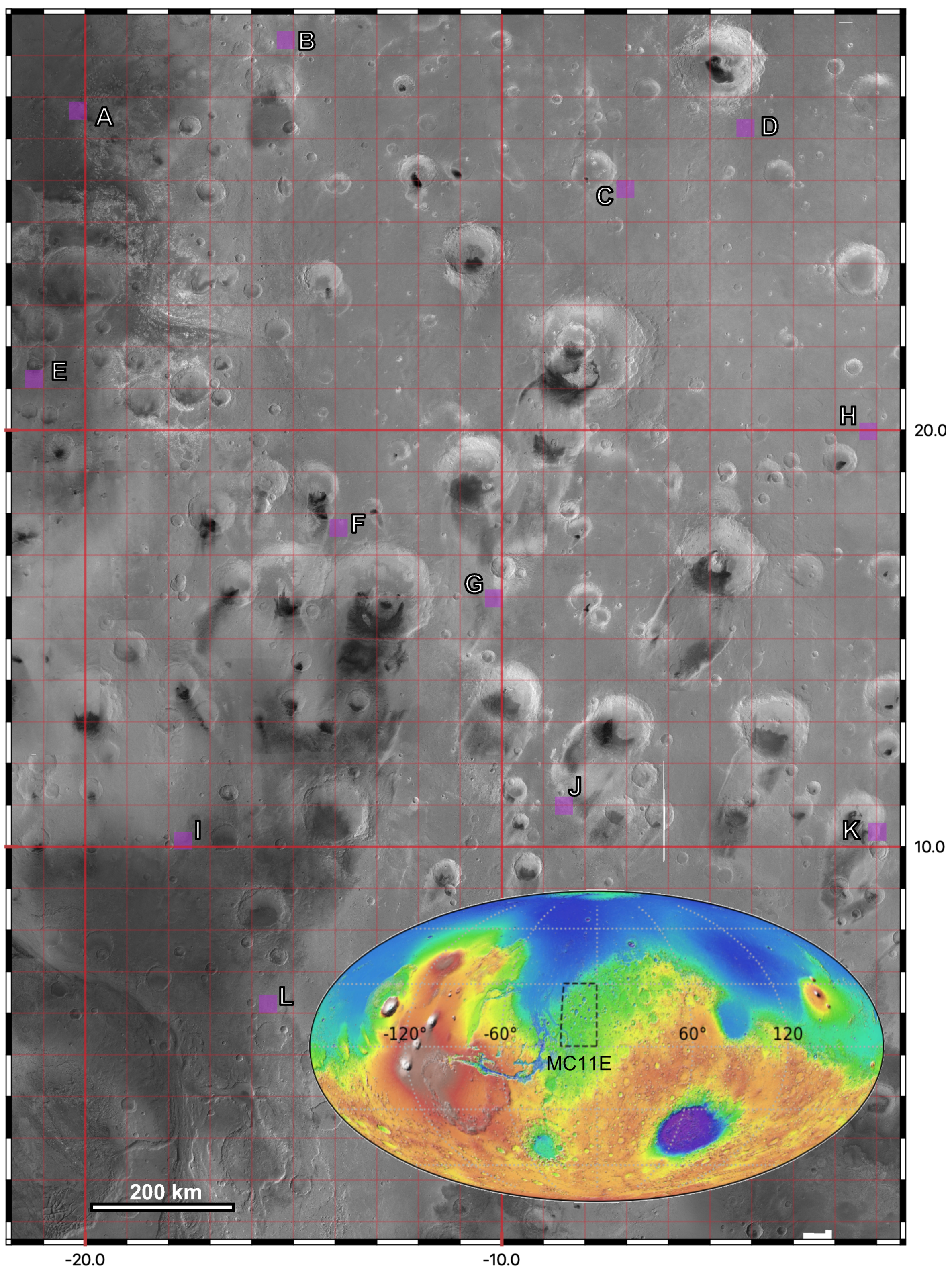
2. Data Description
| <annotation> <folder>data/images/</folder> <filename>MC11E–B.png</filename> <path>data/images/MC11E–B.png</path> <source> <database>MSSL ORBYTS MCC</database> <annotation>MSSL ORBYTS</annotation> <image>NASA CTX / iMars</image> </source> <size> <width>2000</width> <height>2000</height> <depth>1</depth> </size> <segmented>0</segmented> <object> <name>crater</name> <pose>Unspecified</pose> <truncated>0</truncated> <difficult>0</difficult> <bndbox> <xmin>232</xmin> <ymin>224</ymin> <xmax>260</xmax> <ymax>252</ymax> </bndbox> </object> <object> … |
3. Methods
3.1. Collection
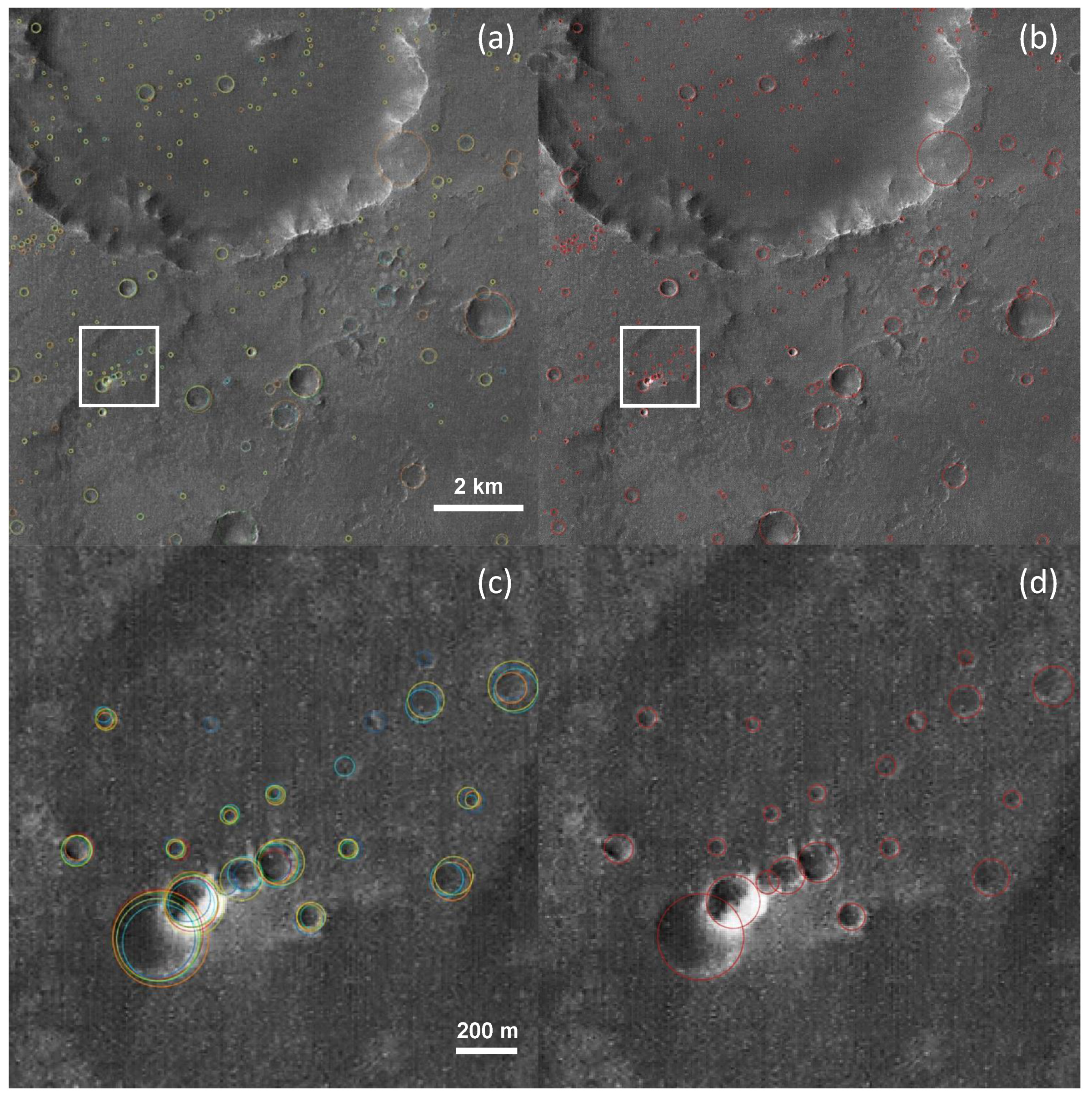
3.2. Validation
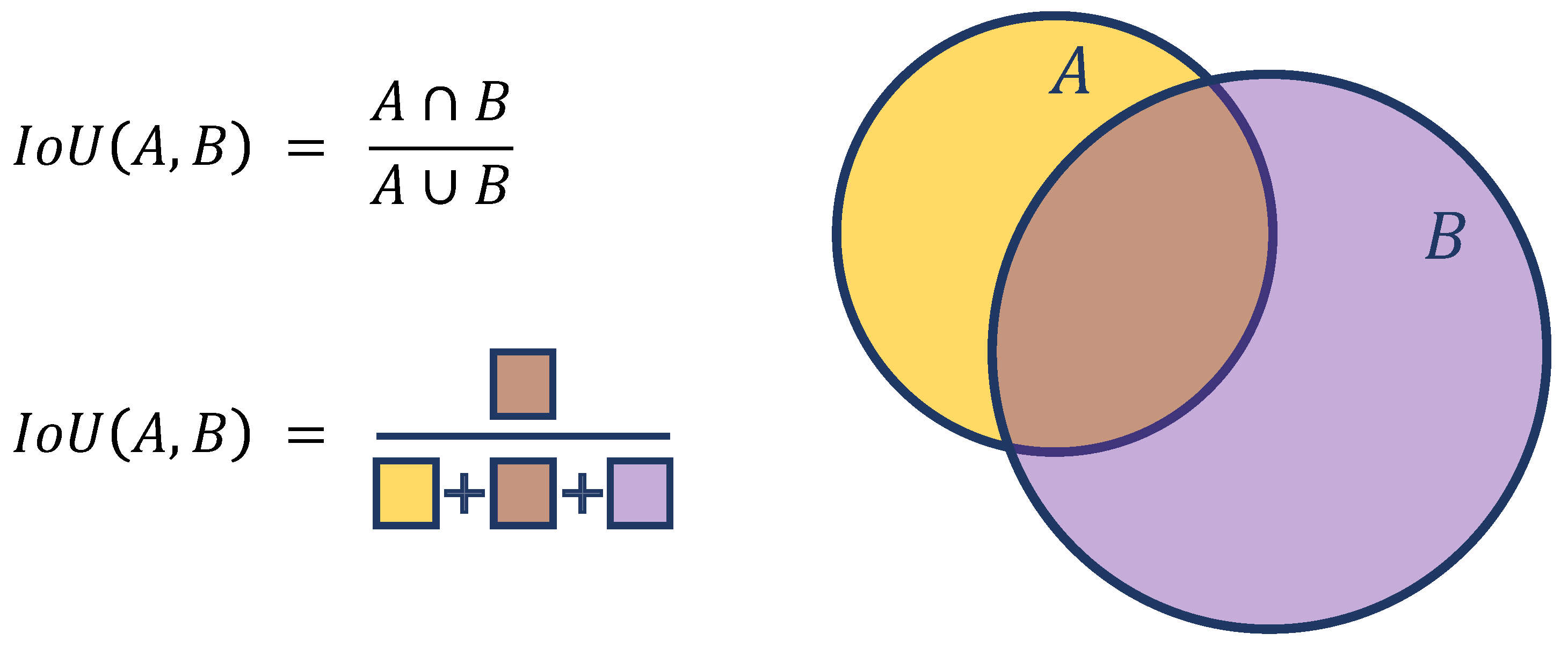
- Let the ith label from annotator n be denoted as .
- For each made by annotator n, compute the intersection-over-union of it with all labels from all other annotators.
- Let the maximum of all these intersection-over-unions be . This is the highest intersection-over-union of one annotator’s label when compared to all other annotations from other annotators.
- Take the mean average of across i, to calculate the nth annotator’s Agreement Score.
4. Discussion
5. User Notes
Author Contributions
Funding
Acknowledgments
Conflicts of Interest
Abbreviations
| CDA | Crater Detection Algorithm |
| CNN | Convolutional Neural Network |
| CSFD | Crater Size-Frequency Distribution |
| CTX | ConTeXt camera |
| HRSC | High Resolution Stereo Camera |
| IoU | Intersection over Union |
| MC-11 | Mars Chart-11 |
| MIoU | Mean Intersection over Union |
| ORBYTS | Original Research By Young Twinkle Students |
| PASCAL VOC | Pattern Analysis, Statistical Modelling and Computational Learning - Visual Object Classes |
References
- Ivanov, B.; Neukum, G.; Wagner, R. Size-frequency distributions of planetary impact craters and asteroids. In Collisional Processes in the Solar System; Springer: Berlin/Heidelberg, Germany, 2001; pp. 1–34. [Google Scholar]
- Barlow, N.G. Crater size-frequency distributions and a revised Martian relative chronology. Icarus 1988, 75, 285–305. [Google Scholar] [CrossRef]
- Williams, J.P.; van der Bogert, C.H.; Pathare, A.V.; Michael, G.G.; Kirchoff, M.R.; Hiesinger, H. Dating very young planetary surfaces from crater statistics: A review of issues and challenges. Meteorit. Planet. Sci. 2018, 53, 554–582. [Google Scholar] [CrossRef]
- Robbins, S.J.; Hynek, B.M. The secondary crater population of Mars. Earth Planet. Sci. Lett. 2014, 400, 66–76. [Google Scholar] [CrossRef]
- McEwen, A.S.; Preblich, B.S.; Turtle, E.P.; Artemieva, N.A.; Golombek, M.P.; Hurst, M.; Kirk, R.L.; Burr, D.M.; Christensen, P.R. The rayed crater Zunil and interpretations of small impact craters on Mars. Icarus 2005, 176, 351–381. [Google Scholar] [CrossRef]
- Robbins, S.J.; Hynek, B.M. Secondary crater fields from 24 large primary craters on Mars: Insights into nearby secondary crater production. J. Geophys. Res. Planets 2011, 116, E10003. [Google Scholar] [CrossRef] [Green Version]
- Robbins, S.J.; Hynek, B.M. A new global database of Mars impact craters ≥ 1 km: 1. Database creation, properties, and parameters. J. Geophys. Res. Planets 2012, 117, E05004. [Google Scholar] [CrossRef]
- Krizhevsky, A.; Sutskever, I.; Hinton, G.E. Imagenet classification with deep convolutional neural networks. In Advances in Neural Information Processing Systems; MIT Press: Cambridge, MA, USA, 2012; pp. 1097–1105. [Google Scholar]
- Ren, S.; He, K.; Girshick, R.; Sun, J. Faster r-cnn: Towards real-time object detection with region proposal networks. In Advances in Neural Information Processing Systems; MIT Press: Cambridge, MA, USA, 2015; pp. 91–99. [Google Scholar]
- Redmon, J.; Farhadi, A. Yolov3: An incremental improvement. arXiv 2018, arXiv:1804.02767. [Google Scholar]
- DeLatte, D.M.; Crites, S.T.; Guttenberg, N.; Tasker, E.J.; Yairi, T. Segmentation Convolutional Neural Networks for Automatic Crater Detection on Mars. IEEE J. Sel. Top. Appl. Earth Obs. Remote Sens. 2019, 12, 2944–2957. [Google Scholar] [CrossRef]
- Lee, C. Automated crater detection on Mars using deep learning. Planet. Space Sci. 2019, 170, 16–28. [Google Scholar] [CrossRef] [Green Version]
- Urbach, E.R.; Stepinski, T.F. Automatic detection of sub-km craters in high resolution planetary images. Planet. Space Sci. 2009, 57, 880–887. [Google Scholar] [CrossRef]
- Cohen, J.P.; Lo, H.Z.; Lu, T.; Ding, W. Crater detection via convolutional neural networks. arXiv 2016, arXiv:1601.00978. [Google Scholar]
- Bandeira, L.; Ding, W.; Stepinski, T.F. Detection of sub-kilometer craters in high resolution planetary images using shape and texture features. Adv. Space Res. 2012, 49, 64–74. [Google Scholar] [CrossRef]
- Jaumann, R.; Neukum, G.; Behnke, T.; Duxbury, T.C.; Eichentopf, K.; Flohrer, J.; Gasselt, S.; Giese, B.; Gwinner, K.; Hauber, E.; et al. The high-resolution stereo camera (HRSC) experiment on Mars Express: Instrument aspects and experiment conduct from interplanetary cruise through the nominal mission. Planet. Space Sci. 2007, 55, 928–952. [Google Scholar] [CrossRef]
- Bugiolacchi, R.; Bamford, S.; Tar, P.; Thacker, N.; Crawford, I.A.; Joy, K.H.; Grindrod, P.M.; Lintott, C. The Moon Zoo citizen science project: Preliminary results for the Apollo 17 landing site. Icarus 2016, 271, 30–48. [Google Scholar] [CrossRef]
- Malin, M.C.; Bell, J.F.; Cantor, B.A.; Caplinger, M.A.; Calvin, W.M.; Clancy, R.T.; Edgett, K.S.; Edwards, L.; Haberle, R.M.; James, P.B.; et al. Context camera investigation on board the Mars Reconnaissance Orbiter. J. Geophys. Res. Planets 2007, 112. [Google Scholar] [CrossRef] [Green Version]
- Michael, G.; Walter, S.; Kneissl, T.; Zuschneid, W.; Gross, C.; McGuire, P.; Dumke, A.; Schreiner, B.; van Gasselt, S.; Gwinner, K.; et al. Systematic processing of Mars Express HRSC panchromatic and colour image mosaics: Image equalisation using an external brightness reference. Planet. Space Sci. 2016, 121, 18–26. [Google Scholar] [CrossRef] [Green Version]
- Sidiropoulos, P.; Muller, J.P.; Watson, G.; Michael, G.; Walter, S. Automatic coregistration and orthorectification (ACRO) and subsequent mosaicing of NASA high-resolution imagery over the Mars MC11 quadrangle, using HRSC as a baseline. Planet. Space Sci. 2018, 151, 33–42. [Google Scholar] [CrossRef]
- Gwinner, K.; Jaumann, R.; Hauber, E.; Hoffmann, H.; Heipke, C.; Oberst, J.; Neukum, G.; Ansan, V.; Bostelmann, J.; Dumke, A.; et al. The High Resolution Stereo Camera (HRSC) of Mars Express and its approach to science analysis and mapping for Mars and its satellites. Planet. Space Sci. 2016, 126, 93–138. [Google Scholar] [CrossRef]
- Zurek, R.W.; Smrekar, S.E. An overview of the Mars Reconnaissance Orbiter (MRO) science mission. J. Geophys. Res. Planets 2007, 112, E05S01. [Google Scholar] [CrossRef] [Green Version]
- Everingham, M.; Van Gool, L.; Williams, C.K.; Winn, J.; Zisserman, A. The pascal visual object classes (voc) challenge. Int. J. Comput. Vis. 2010, 88, 303–338. [Google Scholar] [CrossRef] [Green Version]
- Original research by Young twinkle students (ORBYTS): When can students start performing original research? Phys. Educ. 2017, 53. [CrossRef]
- McQuitty, L.L. Elementary linkage analysis for isolating orthogonal and oblique types and typal relevancies. Educ. Psychol. Meas. 1957, 17, 207–229. [Google Scholar] [CrossRef]
- Michael, G.; Neukum, G. Planetary surface dating from crater size–frequency distribution measurements: Partial resurfacing events and statistical age uncertainty. Earth Planet. Sci. Lett. 2010, 294, 223–229. [Google Scholar] [CrossRef]


| SCENE | Labels per Annotator | Agreement Score (%) | ||||||||||||
|---|---|---|---|---|---|---|---|---|---|---|---|---|---|---|
| i | ii | iii | iv | v | vi | TOTAL | i | ii | iii | iv | v | vi | MEAN | |
| A | 680 | 255 | 396 | 376 | 1111 | 413 | 3231 | 62.4 | 74.8 | 73.5 | 79 | 40.8 | 63.5 | 65.67 |
| B | 88 | 90 | 93 | 151 | 177 | 125 | 724 | 75.5 | 77.7 | 82.1 | 67.9 | 58.7 | 71.7 | 72.27 |
| C | 125 | 212 | 97 | 178 | 230 | 196 | 1038 | 82.6 | 69 | 78.6 | 74.6 | 68.9 | 75.4 | 74.85 |
| D | 72 | 43 | 32 | 94 | 73 | 85 | 399 | 75.7 | 77.1 | 82.3 | 63.9 | 75.7 | 62.9 | 72.93 |
| E | 277 | 503 | 690 | 778 | 869 | 837 | 3954 | 79.2 | 73 | 67.3 | 67.7 | 62.2 | 66.6 | 69.33 |
| F | 197 | 229 | 235 | 278 | 305 | 187 | 1431 | 75.1 | 74.7 | 80.6 | 69.7 | 65.3 | 80.4 | 74.3 |
| G | 45 | 22 | 45 | 45 | 60 | 51 | 268 | 74.9 | 83.2 | 80.0 | 79.5 | 66.2 | 75.7 | 76.58 |
| H | 24 | 36 | 43 | 37 | 40 | 43 | 223 | 86.5 | 78.6 | 74.8 | 83.7 | 72.3 | 77.6 | 78.91 |
| I | 147 | 135 | 174 | 209 | 183 | 262 | 1110 | 68.9 | 77.7 | 75.2 | 68.0 | 73.7 | 52.3 | 69.32 |
| J | 25 | 95 | 32 | 40 | 69 | 36 | 297 | 71.2 | 22.4 | 50.5 | 56.7 | 35.1 | 50.8 | 47.78 |
| K | 66 | 45 | 28 | 63 | 36 | 66 | 304 | 66.8 | 100 | 74.8 | 86.8 | 74.6 | 67.6 | 78.43 |
| L | 375 | 696 | 273 | 281 | 583 | 581 | 2789 | 74.1 | 46.4 | 71.7 | 73.9 | 63.6 | 47.1 | 62.78 |
| TOTAL | 15,768 | 70.26 | ||||||||||||
| Diameter (m) | |||||||
|---|---|---|---|---|---|---|---|
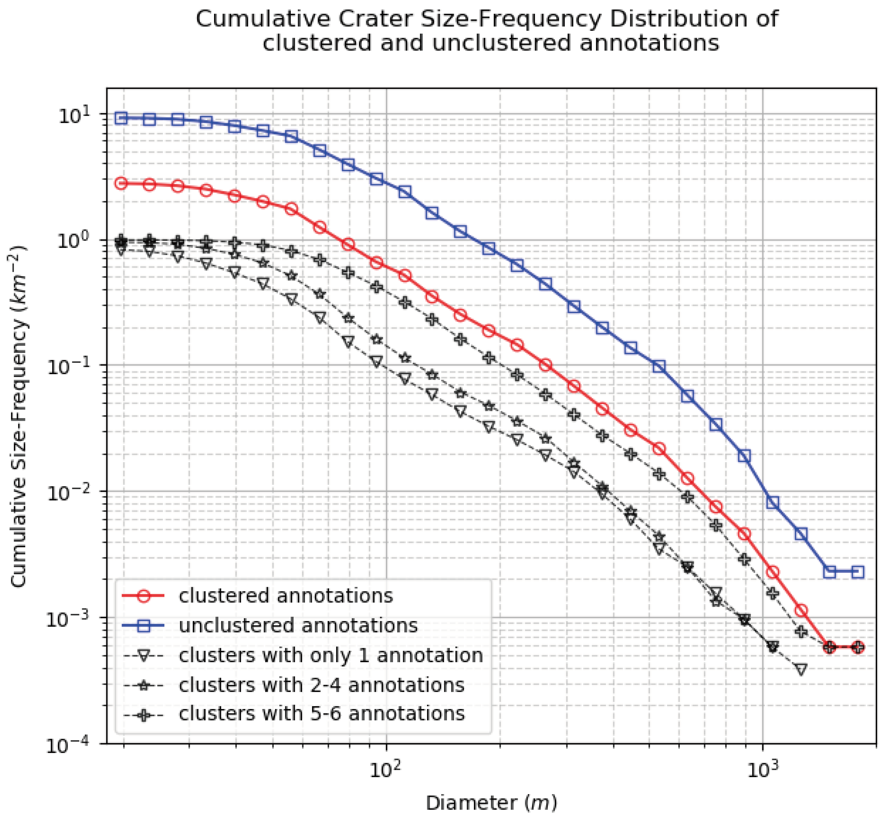
| SCENE | Valid Individual Annotations | Clustered Annotations | Average Annotations per Crater | Median | Mean | Min | Max |
| A | 3230 | 1182 | 2.73 | 60.0 | 66.9 | 18.0 | 366.0 |
| B | 724 | 196 | 3.69 | 108.0 | 136.0 | 36.0 | 918.0 |
| C | 1038 | 269 | 3.86 | 78.0 | 118.8 | 30.0 | 1188.0 |
| D | 397 | 112 | 3.54 | 66.0 | 106.4 | 24.0 | 1152.0 |
| E | 3946 | 1042 | 3.79 | 42.0 | 57.7 | 18.0 | 1938.0 |
| F | 1430 | 372 | 3.84 | 78.0 | 105.4 | 18.0 | 642.0 |
| G | 267 | 72 | 3.71 | 105.0 | 146.4 | 18.0 | 642.0 |
| H | 223 | 60 | 3.72 | 222.0 | 263.3 | 66.0 | 774.0 |
| I | 1110 | 325 | 3.42 | 72.0 | 93.2 | 24.0 | 552.0 |
| J | 297 | 168 | 1.77 | 54.0 | 83.1 | 18.0 | 798.0 |
| K | 304 | 81 | 3.75 | 90.0 | 118.2 | 24.0 | 672.0 |
| L | 2780 | 884 | 3.14 | 60.0 | 64.6 | 18.0 | 630.0 |
| TOTAL | 15,746 | 4763 | 3.31 | 60.0 | 81.1 | 18.0 | 1938.0 |
| No. of Annotations for Crater | No. of Craters | Mean Diameter (m) | Standard Deviation of Diameter (%) | Standard Deviation of Centre (m) |
|---|---|---|---|---|
| 1 | 1442 | 61.8 | - | - |
| 2 | 636 | 68.4 | 16.6 | 4.37 |
| 3 | 524 | 72.1 | 18.1 | 4.87 |
| 4 | 467 | 72.6 | 17.8 | 4.97 |
| 5 | 572 | 82.0 | 16.9 | 5.51 |
| 6 | 1122 | 120.5 | 13.8 | 5.49 |
| SCENE | Non-Expert Annotators | Expert Annotator | ||||||
|---|---|---|---|---|---|---|---|---|
| No. of Labels | Agreement Score (%) | No. of Labels | Agreement Score (%) | |||||
| Min | Max | Mean | Min | Max | Mean | |||
| D | 32 | 94 | 66.5 | 62.9 | 77.1 | 72.9 | 52 | 81.6 |
| F | 187 | 305 | 238.5 | 65.3 | 80.6 | 74.3 | 240 | 81.4 |
| K | 28 | 66 | 50.7 | 66.8 | 100 | 78.4 | 51 | 78.2 |
| L | 273 | 696 | 464.8 | 46.4 | 74.1 | 62.8 | 589 | 69.4 |
© 2020 by the authors. Licensee MDPI, Basel, Switzerland. This article is an open access article distributed under the terms and conditions of the Creative Commons Attribution (CC BY) license (http://creativecommons.org/licenses/by/4.0/).
Share and Cite
Francis, A.; Brown, J.; Cameron, T.; Crawford Clarke, R.; Dodd, R.; Hurdle, J.; Neave, M.; Nowakowska, J.; Patel, V.; Puttock, A.; et al. A Multi-Annotator Survey of Sub-km Craters on Mars. Data 2020, 5, 70. https://0-doi-org.brum.beds.ac.uk/10.3390/data5030070
Francis A, Brown J, Cameron T, Crawford Clarke R, Dodd R, Hurdle J, Neave M, Nowakowska J, Patel V, Puttock A, et al. A Multi-Annotator Survey of Sub-km Craters on Mars. Data. 2020; 5(3):70. https://0-doi-org.brum.beds.ac.uk/10.3390/data5030070
Chicago/Turabian StyleFrancis, Alistair, Jonathan Brown, Thomas Cameron, Reuben Crawford Clarke, Romilly Dodd, Jennifer Hurdle, Matthew Neave, Jasmine Nowakowska, Viran Patel, Arianne Puttock, and et al. 2020. "A Multi-Annotator Survey of Sub-km Craters on Mars" Data 5, no. 3: 70. https://0-doi-org.brum.beds.ac.uk/10.3390/data5030070