Aircraft Engine Run-to-Failure Dataset under Real Flight Conditions for Prognostics and Diagnostics


1
Chair of Intelligent Maintenance Systems, ETH Zürich, 8093 Zürich, Switzerland
2
KBR, Inc., NASA Ames Research Center, Mountain View, CA 94035, USA
3
Operation and Maintenance, Luleå University of Technology, 971 87 Luleå, Sweden
4
PARC, Intelligent Systems Lab, Palo Alto, CA 94043, USA
*
Author to whom correspondence should be addressed.
†
Current address: HIL H 27.3, Stefano-Franscini-Platz 5, 8093 Zürich, Switzerland.
Data 2021, 6(1), 5; https://0-doi-org.brum.beds.ac.uk/10.3390/data6010005
Submission received: 15 December 2020
/
Revised: 7 January 2021
/
Accepted: 8 January 2021
/
Published: 13 January 2021
Abstract
:A key enabler of intelligent maintenance systems is the ability to predict the remaining useful lifetime (RUL) of its components, i.e., prognostics. The development of data-driven prognostics models requires datasets with run-to-failure trajectories. However, large representative run-to-failure datasets are often unavailable in real applications because failures are rare in many safety-critical systems. To foster the development of prognostics methods, we develop a new realistic dataset of run-to-failure trajectories for a fleet of aircraft engines under real flight conditions. The dataset was generated with the Commercial Modular Aero-Propulsion System Simulation (CMAPSS) model developed at NASA. The damage propagation modelling used in this dataset builds on the modelling strategy from previous work and incorporates two new levels of fidelity. First, it considers real flight conditions as recorded on board of a commercial jet. Second, it extends the degradation modelling by relating the degradation process to its operation history. This dataset also provides the health, respectively, fault class. Therefore, besides its applicability to prognostics problems, the dataset can be used for fault diagnostics.
Data Set License: CC0 1.0
1. Introduction
Failures of safety-critical systems such as aircraft engines can cause significant economic disruptions and have potently high social costs. The prediction of the system’s failure time is therefore of great importance for maintaining the functionality of safety-critical systems and society. The problem of predicting how long a particular industrial asset is going to operate until a system failure occurs, i.e., predicting RUL, is also referred to as prognostics [1]. Deploying successful prognostic methods in real-life applications would enable the design of intelligent maintenance strategies to determine with a sufficiently long lead time before failure when interventions need to be performed. Such maintenance strategies have the potential of reducing costs, machine downtime, and the risk of potentially catastrophic consequences if the systems are not maintained in time.
In light of their superior learning capabilities in a wide range of application fields, Machine Learning (ML), in general, and Deep Learning (DL), in particular, are promising candidates to tackle the challenges involved in the design of intelligent maintenance approaches [2]. This idea has been reinforced by the recent availability of large volumes of condition monitoring (CM) data from critical assets. As multiple research studies have pointed out [3,4,5,6,7], the CM data provide an untapped potential to develop data-driven algorithms for various predictive maintenance applications.
The development of data-driven prognostics models requires the availability of datasets with run-to-failure trajectories. These trajectories need to be comprised of a set of time series of CM data along with the corresponding time-to-failure labels. While CM data are often available in abundance, they typically lack the corresponding time-to-failure labels due to the rarity of occurring failures in safety-critical systems and the excessive preventive maintenance. Moreover, due to the sensitive nature of failures and the potential legal implications, manufacturers and operators have been reluctant to share prognostics datasets of their assets openly. As a result, over the last decade, only a very limited number of datasets have been made available to the scientific community for the development of prognostics models. At present, most of the available datasets are synthetic datasets generated with simulators or developed in a lab environment for simple systems by governmental and academic institutions [8,9]. While the availability of even such limited datasets is one of the most relevant contributors to the considerable progress of the prognostics and health management (PHM) in the last decade, these datasets lack important factors of complexity that are present in real systems. As a consequence, the developed data-driven prognostics algorithms are often not transferable to real applications.
Since its release as PHM Challenge [10] in 2008, the CMAPSS dataset [11] has been one of the most widely used prognostics datasets. Some recent examples that are also among the best performing prognostics models applied to the CMAPSS dataset are deep learning based methods such as convolutional neural network (CNN) [12,13], long short-term memory networks (LSTM) [14,15,16,17,18,19] or hybrid networks combining CNN and LSTM layers [20,21]. The CMAPSS dataset provides simulated run-to-failure trajectories of a fleet comprising large turbofan engines. However, the represented flight conditions are restricted to six snapshots during a standard cruise phase, and the onset of an abnormal degradation (i.e., presence of a fault signature) is not dependent on the past operating profile. Therefore, the onset of the fault cannot be predicted; only the evolution of the fault can. Consequently, there is a fidelity gap in the dataset as the simulated degradation trajectories lack important factors of complexity that are present in real engines. Bringing higher fidelity to the degradation and the operating conditions represented in the CMAPSS dataset could improve the usability and the transferability of the developed data-driven models to real-world applications.
In this work, we introduce improvements and further developments to the original CMAPSS dataset with respect to two main aspects. First, we simulate complete flights as recorded on board a commercial jet, covering climb, cruise and descend flight conditions corresponding to different commercial flight routes [22]. Second, we increase the fidelity of degradation modelling by relating the onset of the degradation process to the operation history. To further extend the applicability of this dataset for a range of different case studies, we also include the health condition (i.e., healthy or faulty) in the dataset. We refer to the new CMAPSS dataset as N-CMAPSS. The procedure for generating this dataset is shown schematically in Figure 1 and described in detail in the Methods section.
The new prognostics dataset as proposed here will help to facilitate the development of deep learning algorithms for predictive maintenance applications that are more easily transferable to real applications.
2. Data Description
2.1. CMAPSS Model
An important requirement for the generation of realistic run-to-failure trajectories is the availability of a suitable system model that allows variations of health conditions at sub-system level and the simulation of the output sensor measurements. The CMAPSS dynamical model is a high fidelity computer model for simulation of a realistic large commercial turbofan engine. Figure 2 shows a schematic representation of the engine along with the corresponding station numbers as defined in the CMAPSS model documentation [23]. In addition to the engine thermodynamic model, the package includes an atmospheric model capable of operation at (i) altitudes from sea level to 40,000 ft, (ii) Mach numbers from 0 to 0.90, and (iii) sea-level temperatures from −60 to 103 °F. The package also includes a power-management system that allows the engine to be operated over a wide range of thrust levels throughout the full range of flight conditions.
The CMAPSS system model has the form of a coupled system of nonlinear equations. The inputs of the system model are divided into scenario–descriptor operating conditions w and unobservable model health parameters . The outputs of the system model are estimates of the measured physical properties and unobserved properties that are not part of the condition monitoring signals (i.e., virtual sensors). The nonlinear system model is denoted as:
The unobservable model health parameters are model tuners and fall in the class referred to as quality parameters (i.e., component efficiencies, flow, input scalars, output scalars, and/or adders). These model parameters are used to simulate the deteriorated behaviour of the system. Concretely, in our work, all the rotating sub-components of the engine i.e., fan, low pressure compressor (LPC), high pressure compressor (HPC), low pressure turbine (LPT) and high pressure turbine (HPT) can be affected by degradation in flow and efficiency. In this work, we extended the number of sub-components that can be affected by the degradation from two to five.
2.2. Flight Data
Real flight conditions as recorded on board of a commercial jet were taken as input to the CMAPSS model (i.e., w). We divided the flight conditions in three flight classes according to the flight length. Table 1 shows exemplary the flight length range and the number of different flights in the DASHlink—Flight Data For Tail 687 [22]. It is assumed that each flight of the fleet only operates a particular flight class. Therefore, the assignation of a flight class to each unit is done only once.
Figure 3 (left) shows the kernel density estimations of the simulated flight envelopes given by the scenario–descriptor variables w: altitude (alt), flight Mach number (Mach), throttle–resolver angle (TRA) and total temperature at the fan inlet (T2) for dataset DS02. An example of a typical single flight cycle given by traces of the scenario–descriptor variables is shown in Figure 3 (right). Each flight cycle contains recordings of varying lengths, covering climb, cruise and descend flight conditions (with 10,000 ft) corresponding to different flight routes operated by the aircraft. The remaining units of the fleet follow similar flight traces.
2.3. Data Records
The N-CMAPSS dataset provides synthetic run-to-failure degradation trajectories of a fleet of turbofan engines with unknown initial health states subject to real flight conditions. At present, the N-CMAPSS dataset contains eight sets of data from 128 units and seven different failure modes affecting the flow (F) and/or efficiency (E) of all the rotating sub-components. Table 2 provides an overview of flight classes and failure modes for each of the sets of data provided. Each set of data are stored in a Hierarchical Data Format version 5 (HDF5) file1. The dataset is accessible publicly at the repository: https://ti.arc.nasa.gov/tech/dash/groups/pcoe/prognostic-data-repository/. Scripts in the form of Jupyter notebooks are available also in the data repositories to demonstrate how to load the data, reproduce the analysis of this manuscript and to apply simple analysis to subvolumes of data. The online dataset will be updated when new degradation trajectories are computed.
Each data file provides two sets of data: the development dataset and the test dataset. Each of them contains six types of variables: the operative conditions w, the measured signals , the virtual sensors , the engine health parameters , the RUL label and the auxiliary data (i.e., the unit number u and the flight cycle number c, the flight class and the health state ). In addition, the name of the variables within w, and , and the auxiliary data are provided. Table 3 shows an overview of the 17 variables stored in the .h5 file.
Table 4, Table 5, Table 6, Table 7 and Table 8 provide the name, description and units of each input variable in the dataset. The variable symbol corresponds to the internal variable name in the CMAPSS model. The descriptions and units are derived from the model documentation [23]. RUL is provided in units of cycles.
3. Methods
The method used for generation of the N-CMAPSS dataset follows the methodology delineated in [11] and depicted in Figure 1. In brief, the method corresponds to the following process:
- Define flight conditions. Real flight conditions as recorded on board of a commercial jet (i.e., NASA DASHlink [22] data) are taken as input to an engine simulator.
- Impose degradation. Degradation of the engine components is imposed at each flight.
- Simulation of a degraded flight. Complete flight covering climb, cruise and descend conditions is simulated with the CMAPSS dynamical model [23].
- Flight until failure. As a result of the degradation of the engines’ components, the health state of the engine decreases. The simulation of full flights (steps 1–3) with increasing degradation continues until the health index of the engine has reached zero i.e., ; which defines the end-of-life.
- Add sensor noise. Sensor noise is added to the simulated data to account for the variability of real sensor readings.
In the following, we describe the key steps of the data generation process outlined above in more detail.
3.1. Degradation Model
The degradation of each engine is modelled as the combination of three contributors: an initial degradation, a normal degradation and abnormal degradation. The dataset generation process assumes failure modes exhibiting a continuous degradation of the main rotating engine sub-components: fan, LPC, HPC, HPT and LPT. The degradation effects are modelled by adjustments of flow capacity and efficiency of these engine sub-components (i.e., the engine health parameters ).
Initial degradation. Due to manufacturing and assembly tolerances, each unit of the fleet has sightly different initial wear at the engine sub-component. Degradation due to this initial wear is not considered abnormal but can make a difference in useful operational life of a component. Following the original work, this initial wear is modeled by variations in flow and efficiencies of the various sub-component. An uniform random distribution is assumed for each of the sub-components. The magnitude of such variations is relatively low, resulting in a health index within the range [0.9 to 1.0]. We denote the initial degradation as .
Normal degradation. In addition to the initial wear, the system’s components also experience degradation due to wear and tear resulting from usage. This type of degradation is considered normal and is modelled as linear decreasing trend given by:
where is the slope of the degradation, and t refers to the time in units of cycles, i.e., flights.
Transition from normal to abnormal degradation. Some time during an engine’s life, its health state might transition to an abnormal state resulting from the presence of a particular failure mode. That is, at a point in time, , the corresponding fault leads to an abnormal condition and to an eventual failure at (i.e., end-of-life). We model the onset of a fault as a stochastic process governed by past operation history. While the detailed computation of the micro-level processes leading to a degraded state was not within the scope of this analysis, we capture the macro-level degradation characteristics leading to a fault by computing the energy balances around each sub-component. Concretely, it is assumed that each sub-component can only withstand certain excitation energy before reaching a state of abnormal degradation. We denote the maximum excitation energy of sub-component as , which we model as a Gaussian distribution to represent variability on the material properties of each unit. The fault onset time corresponds to the point in time at which the total amount of energy E that a component has been exited with from an initial time to a time t exceeds . i.e., . The excitation energy experienced by a sub-component in the time interval is given by:
where is the power consumed or produced by each component.
Abnormal degradation. The evolution of the abnormal system degradation with time follows the modelling of the original work. In brief, the abnormal degradation model assumes the degradation of each system sub-components flow and efficiencies (i.e., ) is governed by the following model:
where , and is the process noise with when corresponds to an efficiency and to a flow capacity.
Since a, b and are random variables, the evolution of the abnormal degradation with time is stochastic. The degradation process follows an exponential behaviour common in multiple damage propagation models (e.g., Arrhenius, Coffin–Manson, and Eyring models). Concretely, the modelling assumes a generalized equation for wear, , which ignores micro-level deterioration processes but retains macro-level degradation characteristics. The between-flight maintenance is not explicitly modeled but is considered by the process noise. This allows the engine health parameters (flow and efficiency) to improve within allowable limits at any point and hence the loss in efficiency or flow is not locally monotonic (see step 2 in Figure 1).
3.2. Health Condition
The modelling approach assumes an overall health index of the engine i.e., . The health index of the engine is monitored at each flight, and the end of life is declared when the health index reaches a zero value i.e., or the system has reached more that 100 operative cycles. The overall health index is modelled as aggregation of four normalized remaining operative margins () that characterize the wear/health of the engine:
In particular, the surge margins of the fan (), LPC () and HPC () and the exhaust gas temperature () computed at reference conditions2 are the operative margins considered that we denote as . Delta differences of these operative margins between a degraded engine and the corresponding values of a clean new engine are assumed as measures of wear i.e., . Furthermore, the degradation model assumes upper wear thresholds, , that denote the operational limits beyond which the engine cannot be operated. Under this assumption, the evolution of the normalized remaining operative margins with time, , for each of the operative margins monitored is obtained by subtracting the wear from an upper threshold and normalizing it with respect to the upper threshold:
3.3. Sensor Noise
Measurement noise is an important source of variability present in real systems. A typical approach to model it is to add the white noise model to the simulated response. In this study, since there were no real data available to characterize true noise levels, we added Gaussian noise to the signals with a target Signal-to-Noise Ratio (SNR) target of 65 dB. With this noise intensity, the resulting noise level is in alignment with the measurement uncertainties reported in the literature for modern turbofan engines [24,25]. It should be noted that the flight conditions (w) contain already sensor noise since they are real flight data.
3.4. Technical Validation
Quality assurance and quality control of the provided data included the following steps performed by different teams. First, one team checked if the flight profiles were within the flight envelope of the CMAPSS dynamical model. Second, an independent team assessed whether the generated degradation profiles from the different dataset showed the intended characteristics: random initial wear, linear normal degradation, sharp abnormal degradation and smooth transition from normal to abnormal degradation. Finally, all the authors checked if the outputs of the engine model follow the expected behavior and are bounded by physically meaningful upper/lower values. In the following, we provide a closer look at some of these important aspects of the data generation process.
3.4.1. Examination of the Flight Profiles
All flight data were checked to ensure that only flight conditions within the validity of the simulation flight envelope of the CMAPSS model were used. Figure 4 shows the simulated flight envelopes given by the scenario–descriptor variables altitude (alt), flight Mach number (XM) of ten units in dataset DS01 color coded by the flight class. It is worth noticing that each of the three flight classes has different operation profiles. In particular, flight class 1 (green) represents short flights (1–3 h) at low altitude and speed. Fight class 2 (orange) constitutes longer flights (3–5 h) at higher altitudes. Fight class 3 is flights that have the longest (5–7 h) and highest flights compared to the other flight classes. All the simulated flights are contained within the operation envelope of the CMAPSS dynamical model, and, therefore, are valid flight profiles for simulation.
3.4.2. Examination of the Degradation Trajectories
The degradation trajectories generated are designed to show three characteristics present in real systems: random initial wear, linear normal degradation, and abnormal degradation. Figure 5 shows the resulting evolution of the health index (i.e., ) in the ten units of dataset DS01. We can observe that the initial deterioration of each unit is different and corresponds to an engine-to-engine variability equivalent to a 10% of the health index. The degradation of the affected system components follows a stochastic process with a linear normal degradation followed by a steeper abnormal degradation. The transition from normal to abnormal degradation is smooth. The degradation rate of each component varies within the fleet.
3.4.3. Examination of the Transition Times
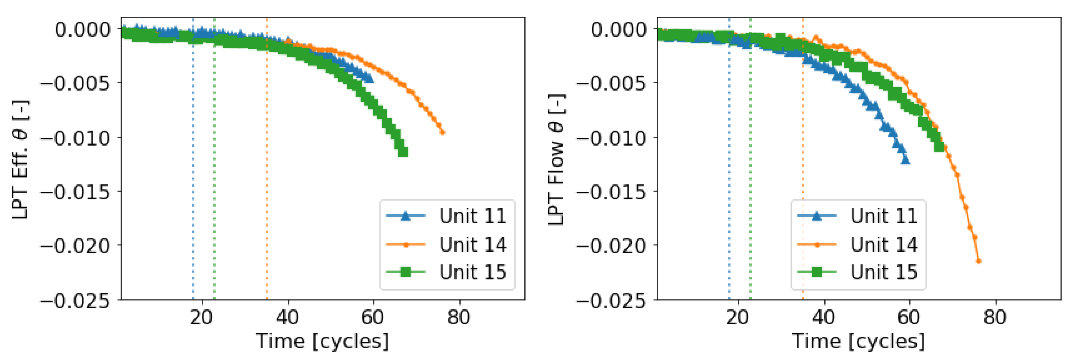
The transition time () is dependent on the operating conditions i.e., flight profile. To illustrate the impact of the operative conditions on the onset of the abnormal degradation, Figure 6 shows the traces of degradation imposed on the high pressure turbine efficiency (HPT_Eff_mod), low pressure turbine efficiency (LPT_Eff_mod) and low pressure turbine flow (LPT_flow_mod) on three units of DS02. Each of the selected units correspond to a different flight class. Unit 11 is long flight unit (i.e., flight class 3), and the onset of the abnormal degradation occurs the earliest at 19 cycles. Unit 14 is short flight length unit (i.e., flight class 1) and has an onset at 36 cycles. Finally, Unit 15 is medium flight length unit (i.e., flight class 2) and has an onset at 24 cycles. We can observe that abnormal degradation arises later in Unit 14 and consequently can perform more flights.
In addition to the quality assurance and quality control checks, two of the sets of data provided have been satisfactorily used in previous works. Specifically, dataset DS01 has been used for the application of model-based diagnostics [26] and dataset DS02 has been used for data-driven prognostics [27].
4. Usage Notes
The N-CMAPSS has the potential to facilitate the development of DL algorithms for predictive maintenance applications that are more easily transferable to real-world applications. The dataset can also serve as a benchmark enabling a better comparison of different algorithms and their extensions. Moreover, the N-CMAPSS dataset is a resource for the machine learning community to test new time-dependent algorithms. It should be noted that, contrarily to the original CMAPSS work, the N-CMAPSS provides the degradation trajectories in the form of . Therefore, the N-CMAPSS dataset can also be used to develop new physics-informed machine learning algorithms [28]. We conclude by providing a brief abstract formulation of prognostics and diagnostics problems aiming at facilitating the understanding of both problems to a larger scientific audience.
4.1. Prognostics Problem
Multivariate time-series of condition monitoring sensors readings are given and their corresponding RUL i.e., from a fleet of N units (). Each observation is a vector of p raw measurements taken at operating conditions . The length of the sensory signal for the i-th unit is given by , which can, in general, differ from unit to unit. The total combined length of the available data set is . More compactly, we denote the available dataset as . Given this set-up, the task is to obtain a predictive model that provides a reliable RUL estimate () on a test dataset of M units , where are multivariate time-series of sensors readings. The total combined length of the test data set is .
Evaluation Metric
Two common evaluation metrics in CMAPSS prognostics analysis in [11] are proposed to compare the prognostics results: root-mean-square error (RMSE) and NASA’s scoring function [11] (s), which are defined as:
where denotes the total number of test data samples, is the difference between the estimated and the real RUL of the j sample (i.e., ), and is if RUL is under-estimated and , otherwise. The resulting s metric is not symmetric and penalizes over-estimation more than under-estimation.
4.2. Diagnostics Problem
The formulation of the suggested diagnostic problem is formally introduced in the following. Multivariate time-series of condition monitoring sensors readings are given from a fleet of N units (). Each observation is a vector of p raw measurements taken at operating conditions . The length of the sensory signal for the u-th unit is given by , which can, in general, differ from unit to unit. The total combined length of the available data set is . We consider the situation where the CM data correspond to past operating conditions (i.e., ), where the system’s health state is healthy and denoted as with . Therefore, in compact form, we denote the available unit specific data as . The system’s components experience normal degradation during the healthy state. We consider the scenario where this normal degradation turns into an abnormal condition at leading to an eventual failure at (i.e., end-of-life). The fault detection task is to detect as early as possible the onset of the abnormal degradation within an independent test data set of future operating conditions (i.e., ). This task comprises, therefore, the estimation of the true system health state on the test set. In addition, the diagnostics task involves performing a fault isolation and identifying the subsystem(s) affected by the fault.
5. Discussion
In this work, we provide a new CMAPSS dataset (N-CMAPSS) with run-to-failure degradation trajectories that incorporate two major fidelity improvements with respect to previous work. First, it considers real flight conditions as recorded on board a commercial jet. Second, it extends the degradation modelling by relating the degradation process to its operation history. The N-CMPASS dataset also provides fault class labels of each failure mode. Therefore, besides its applicability to prognostics problems, the dataset can be used for fault diagnostics. However, besides these notable improvements, the degradation process of turbofan engines can still be improved further and modelled with higher fidelity. In particular, we have considered an accelerated aging as compared to typical engines with full operative lifespans on the order of thousands of cycles. In addition, we have restricted the degradation modelling to certain fault types that can be represented by flow and efficiency modulation. Therefore, extending the represented fault types and the onboard sensors (e.g., accelerometers, oil debris monitoring, etc.) are natural extensions of the work.
Author Contributions
Conceptualization, M.A.C., C.K., K.G. and O.F.; methodology, M.A.C., C.K., K.G. and O.F.; software, M.A.C.; validation, M.A.C. and C.K.; formal analysis, M.A.C., C.K., K.G. and O.F.; investigation, M.A.C. and C.K.; resources, C.K., K.G. and O.F.; data curation, M.A.C.; writing—original draft preparation, M.A.C.; writing—review and editing, M.A.C., C.K., K.G. and O.F.; visualization, M.A.C.; supervision, K.G. and O.F.; project administration, K.G. and O.F.; funding acquisition, O.F. All authors have read and agreed to the published version of the manuscript.
Funding
This research was funded by the Swiss National Science Foundation (SNSF) Grant No. PP00P2 176878.
Institutional Review Board Statement
Not applicable.
Informed Consent Statement
Not applicable.
Data Availability Statement
The data presented in this study are available in: https://ti.arc.nasa.gov/tech/dash/groups/pcoe/prognostic-data-repository/.
Acknowledgments
The authors also thank NASA Ames Research Center for hosting a research stay that allowed development of the N-CMAPSS model and collection of this dataset.
Conflicts of Interest
The authors declare no conflict of interest.
References
- Goebel, K.; Daigle, M.; Saxena, A.; Roychoudhury, I.; Sankararaman, S. Prognostics: The Science of Making Predictions; Createspace Independent Publishing Platform: Scotts Valley, CA, USA, 2017. [Google Scholar]
- Fink, O.; Wang, Q.; Svensén, M.; Dersin, P.; Lee, W.J.; Ducoffe, M. Potential, challenges and future directions for deep learning in prognostics and health management applications. Eng. Appl. Artif. Intell. 2020, 92, 103678. [Google Scholar]
- Lei, Y.; Li, N.; Guo, L.; Li, N.; Yan, T.; Lin, J. Machinery health prognostics: A systematic review from data acquisition to RUL prediction. Mech. Syst. Signal Process. 2018, 104, 799–834. [Google Scholar]
- Hu, C.; Youn, B.D.; Wang, P.; Yoon, J.T. Ensemble of data-driven prognostic algorithms for robust prediction of remaining useful life. Reliab. Eng. Syst. Saf. 2012, 103, 120–135. [Google Scholar]
- Zhang, C.; Lim, P.; Qin, A.K.; Tan, K.C. Multiobjective deep belief networks ensemble for remaining useful life estimation in prognostics. IEEE Trans. Neural Netw. Learn. Syst. 2016, 28, 2306–2318. [Google Scholar] [PubMed]
- Booyse, W.; Wilke, D.N.; Heyns, S. Deep digital twins for detection, diagnostics and prognostics. Mech. Syst. Signal Process. 2020, 140, 106612. [Google Scholar]
- Da Costa, P.R.d.O.; Akcay, A.; Zhang, Y.; Kaymak, U. Remaining useful lifetime prediction via deep domain adaptation. Reliab. Eng. Syst. Saf. 2020, 195, 106682. [Google Scholar]
- Eker, Ö.F.; Camci, F.; Jennions, I.K. Major challenges in prognostics: Study on benchmarking prognostic datasets. In Proceedings of the 1st European Conference of the Prognostics and Health Management Society 2012, Dresden, Germany, 3–6 July 2012; Volume 3, p. 8. [Google Scholar]
- Prognostics Center of Excellence—Data Repository. 2020. Available online: https://ti.arc.nasa.gov/tech/dash/groups/pcoe/prognostic-data-repository/ (accessed on 23 April 2019).
- Saxena, A.; Goebel, K. PHM08 Challenge Data Set. 2008. Available online: https://ti.arc.nasa.gov/tech/dash/groups/pcoe/prognostic-data-repository/ (accessed on 23 April 2019).
- Saxena, A.; Goebel, K.; Simon, D.; Eklund, N. Damage propagation modeling for aircraft engine run-to-failure simulation. In Proceedings of the 2008 International Conference on Prognostics and Health Management, Denver, CO, USA, 6–9 October 2008; pp. 1–9. [Google Scholar] [CrossRef]
- Li, X.; Ding, Q.; Sun, J.Q. Remaining useful life estimation in prognostics using deep convolution neural networks. Reliab. Eng. Syst. Saf. 2018, 172, 1–11. [Google Scholar]
- Yang, H.; Zhao, F.; Jiang, G.; Sun, Z.; Mei, X. A Novel Deep Learning Approach for Machinery Prognostics Based on Time Windows. Appl. Sci. 2019, 9, 4813. [Google Scholar] [CrossRef] [Green Version]
- De Oliveira da Costa, P.R.; Akcay, A.; Zhang, Y.; Kaymak, U. Attention and long short-term memory network for remaining useful lifetime predictions of turbofan engine degradation. Int. J. Progn. Health Manag. 2019, 10, 034. [Google Scholar]
- Listou Ellefsen, A.; Bjørlykhaug, E.; Æsøy, V.; Ushakov, S.; Zhang, H. Remaining useful life predictions for turbofan engine degradation using semi-supervised deep architecture. Reliab. Eng. Syst. Saf. 2019, 183, 240–251. [Google Scholar] [CrossRef]
- Remaining Useful Life Prediction of Airplane Engine Based on PCA–BLSTM. Sensors 2020, 20, 4537. [CrossRef]
- Shi, Z.; Chehade, A. A dual-LSTM framework combining change point detection and remaining useful life prediction. Reliab. Eng. Syst. Saf. 2021, 205, 107257. [Google Scholar] [CrossRef]
- Wu, J.; Hu, K.; Cheng, Y.; Zhu, H.; Shao, X.; Wang, Y. Data-driven remaining useful life prediction via multiple sensor signals and deep long short-term memory neural network. ISA Trans. 2020, 97, 241–250. [Google Scholar] [PubMed]
- Xia, T.; Song, Y.; Zheng, Y.; Pan, E.; Xi, L. An ensemble framework based on convolutional bi-directional LSTM with multiple time windows for remaining useful life estimation. Comput. Ind. 2020, 115, 103182. [Google Scholar]
- Zhao, C.; Huang, X.; Li, Y.; Yousaf Iqbal, M. A Double-Channel Hybrid Deep Neural Network Based on CNN and BiLSTM for Remaining Useful Life Prediction. Sensors 2020, 20, 7109. [Google Scholar] [CrossRef]
- Xie, Z.; Du, S.; Lv, J.; Deng, Y.; Jia, S. A Hybrid Prognostics Deep Learning Model for Remaining Useful Life Prediction. Electronics 2020, 10, 39. [Google Scholar] [CrossRef]
- DASHlink—Flight Data For Tail 687. 2012. Available online: https://c3.nasa.gov/dashlink/resources/664/ (accessed on 23 January 2019).
- Frederick, D.K.; Decastro, J.A.; Litt, J.S. User’s Guide for the Commercial Modular Aero-Propulsion System Simulation (C-MAPSS); Technical Report; NASA: Washington, DC, USA, 2007.
- Kobayashi, T.; Simon, D.L. Evaluation of an Enhanced Bank of Kalman Filters for In-Flight Aircraft Engine Sensor Fault Diagnostics. J. Eng. Gas Turbines Power 2005, 127, 497–504. [Google Scholar] [CrossRef] [Green Version]
- Borguet, S.; Leónard, O. A Generalised Likelihood Ratio Test for Adaptive Gas Turbine Health Monitoring. In Proceedings of the ASME Turbo Expo 2008: Power for Land, Sea, and Air, Berlin, Germany, 9–13 June 2008. [Google Scholar] [CrossRef]
- Tian, Y.; Arias Chao, M.; Kulkarni, C.; Goebel, K.; Fink, O. Real-Time Model Calibration with Deep Reinforcement Learning. arXiv 2020, arXiv:2006.04001. [Google Scholar]
- Arias Chao, M.; Kulkarni, C.; Goebel, K.; Fink, O. Fusing Physics-based and Deep Learning Models for Prognostics. arXiv 2020, arXiv:2003.00732. [Google Scholar]
- Willard, J.; Jia, X.; Xu, S.; Steinbach, M.; Kumar, V. Integrating Physics-Based Modeling with Machine Learning: A Survey. arXiv 2020, arXiv:2003.04919. [Google Scholar]
| 1 | DS08 is provided in five separate files i.e., DS08a-DS08e for easier handling. |
| 2 | i.e., altitude = 20 Kft, flight match number = 0.7, and throttle–resolver angle = 100%. |
Figure 1.
Generation process of the new CMAPSS dataset (i.e., N-CMAPSS) based on the real flight data. First, we define the flight data as recorded on board of a commercial jet. Second, the degradation of the engine components is imposed. Third, the resulting degraded flight is simulated. Fourth, the health condition is evaluated and the unit continues flying with increasing degradation until the health index of the engine has reached zero i.e., , which defines the end-of-life. Finally, sensor noise is added to the simulated engine response.
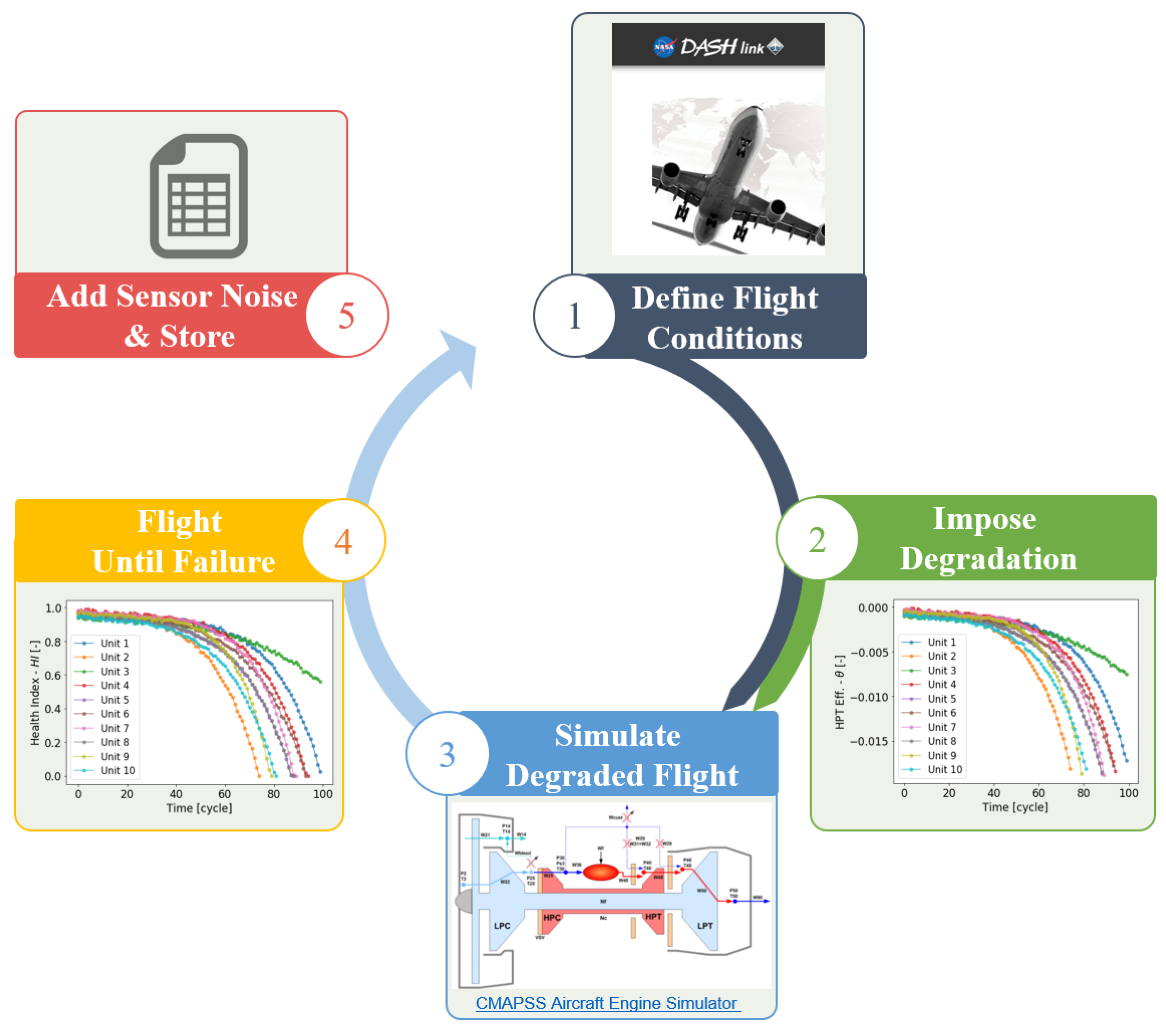
Figure 2.
Schematic representation of the CMAPSS model as depicted in the CMAPSS documentation [23].
Figure 2.
Schematic representation of the CMAPSS model as depicted in the CMAPSS documentation [23].

Figure 3.
(Left) Kernel density estimations of the simulated flight envelopes given by recordings of altitude, flight Mach number, throttle–resolver angle (TRA) and total temperature at the fan inlet (T2). The complete run-to-failure trajectories of the nine units in DS02 are shown. Six training units (2, 5, 10, 16, 18 & 20) and three test units (11, 14 & 15) are represented. (Right) Single flight traces of altitude, flight Mach number (XM), throttle–resolver angle (TRA) and total temperature at the fan inlet (T2) for Unit 5 in DS02. Climb, cruise and descend flight conditions (10,000 ft) are covered.
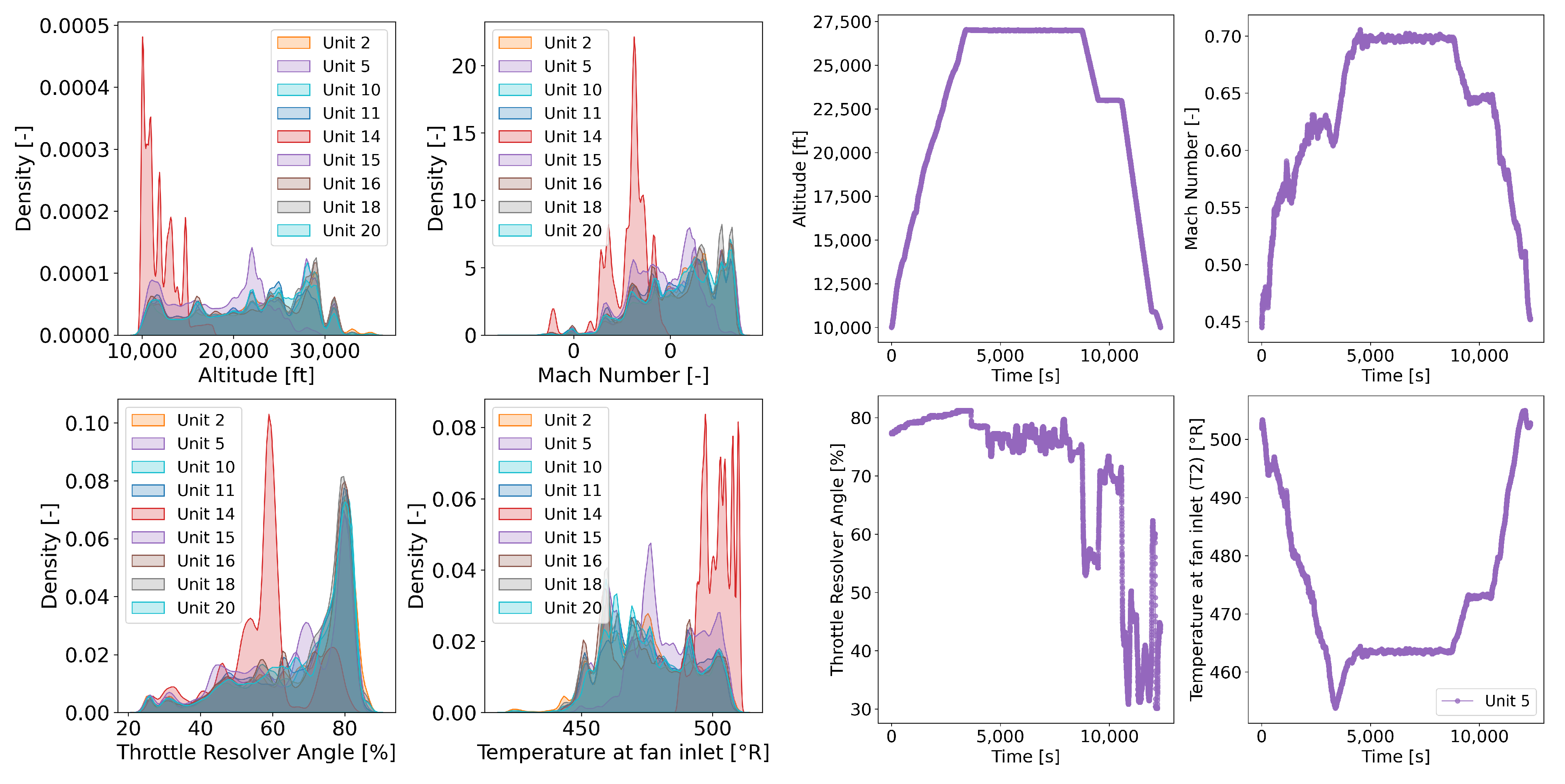
Figure 4.
Real flight envelopes given by recordings of altitude and flight Mach number. The complete run-to-failure trajectories of ten fleet units are shown. The three flight classes are represented: flight class 1 (green), flight class 2 (orange), and flight (blue), The shaded area (light blue) denotes the acceptable operation envelope of the CMAPSS dynamical mode according to the CMAPSS documentation [23].
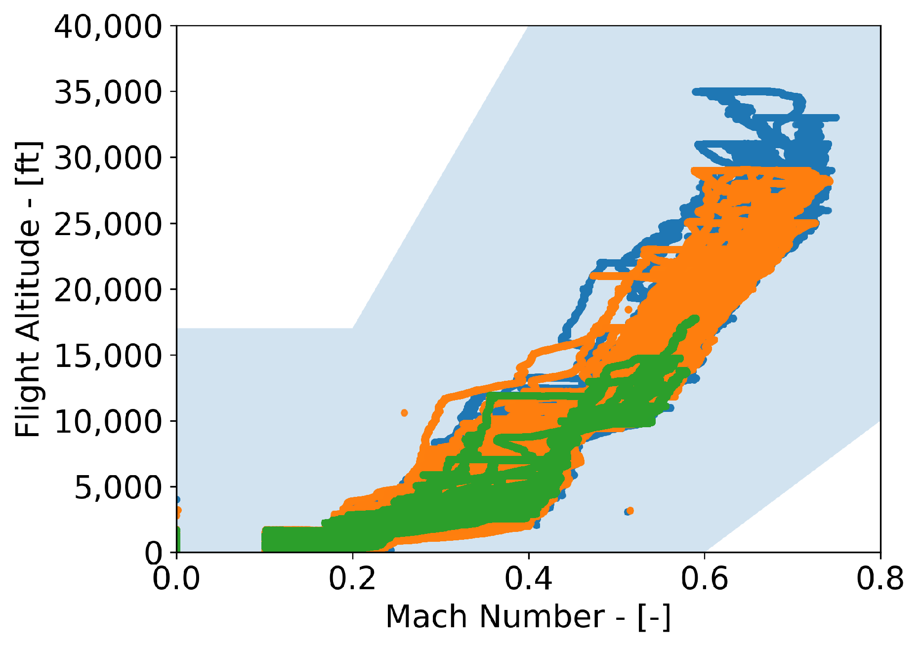
Figure 5.
Evolution of the health index with time as a result of the degradation induced in the HPT in the ten units of dataset DS01.
Figure 5.
Evolution of the health index with time as a result of the degradation induced in the HPT in the ten units of dataset DS01.
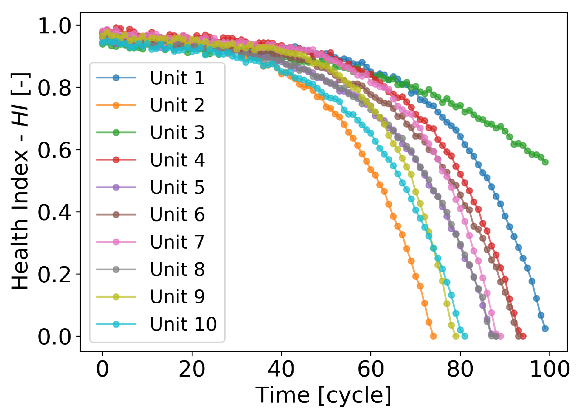
Figure 6.
Traces of the degradation imposed on the low pressure turbine efficiency (LPT_Eff_mod) and low pressure turbine flow (LPT_flow_mod). Three units are shown: Unit 11 (blue triangle), Unit 14 (green square) and Unit 15 (orange circle). The onset of the abnormal degradation (i.e., ) is indicated with dashed vertical lines.


Table 1.
Overview of the flight data in DASHlink—Flight Data For Tail 687 [22].
Table 1.
Overview of the flight data in DASHlink—Flight Data For Tail 687 [22].
| Flight Class | Flight Length [h] | Number of Flights [#] |
|---|---|---|
| 1 | 1 to 3 | 18 |
| 2 | 3 to 5 | 149 |
| 3 | >5 | 185 |
Table 2.
Overview of the datasets.
| Name | # Units | Flight Classes | Failure Modes | Fan | LPC | HPC | HPT | LPT | Size | |||||
|---|---|---|---|---|---|---|---|---|---|---|---|---|---|---|
| E | F | E | F | E | F | E | F | E | F | |||||
| DS01 | 10 | 1, 2, 3 | 1 | ✓ | 7.6 M | |||||||||
| DS02 | 9 | 1, 2, 3 | 2 | ✓ | ✓ | ✓ | 6.5 M | |||||||
| DS03 | 15 | 1, 2, 3 | 1 | ✓ | ✓ | ✓ | 9.8 M | |||||||
| DS04 | 10 | 2, 3 | 1 | ✓ | ✓ | 10.0 M | ||||||||
| DS05 | 10 | 1, 2, 3 | 1 | ✓ | ✓ | 6.9 M | ||||||||
| DS06 | 10 | 1, 2, 3 | 1 | ✓ | ✓ | ✓ | ✓ | 6.8 M | ||||||
| DS07 | 10 | 1, 2, 3 | 1 | ✓ | ✓ | 7.2 M | ||||||||
| DS08 | 54 | 1, 2, 3 | 1 | ✓ | ✓ | ✓ | ✓ | ✓ | ✓ | ✓ | ✓ | ✓ | ✓ | 35.6 M |
Table 3.
Variable names in .h5 files.
| Development Data () | |
|---|---|
| Name | Description |
| W_dev | Scenario descriptors—w |
| X_s_dev | Measurements— |
| X_v_dev | Virtual sensor— |
| T_dev | Health Parameters— |
| Y_dev | [in cycles] |
| A_dev | Auxiliary data |
| Test Data () | |
| Name | Description |
| W_test | Scenario descriptors -w |
| X_s_test | Measurements— |
| X_v_test | Virtual sensor— |
| T_test | Health Parameters— |
| Y_test | [in cycles] |
| A_test | Auxiliary data |
| Variables Name | |
| Name | Description |
| W_var | w variables |
| X_s_var | variables |
| X_v_var | variables |
| T_var | variables |
| A_var | Auxiliary variables |
Table 4.
Scenario descriptors (i.e., flight data)—w.
| # | Symbol | Description | Units |
|---|---|---|---|
| 1 | alt | Altitude | ft |
| 2 | Mach | Flight Mach number | - |
| 3 | TRA | Throttle–resolver angle | % |
| 4 | T2 | Total temperature at fan inlet | °R |
Table 5.
Measurements—.
| # | Symbol | Description | Units |
|---|---|---|---|
| 1 | Wf | Fuel flow | pps |
| 2 | Nf | Physical fan speed | rpm |
| 3 | Nc | Physical core speed | rpm |
| 4 | T24 | Total temperature at LPC outlet | °R |
| 5 | T30 | Total temperature at HPC outlet | °R |
| 6 | T48 | Total temperature at HPT outlet | °R |
| 7 | T50 | Total temperature at LPT outlet | °R |
| 8 | P15 | Total pressure in bypass-duct | psia |
| 9 | P2 | Total pressure at fan inlet | psia |
| 10 | P21 | Total pressure at fan outlet | psia |
| 11 | P24 | Total pressure at LPC outlet | psia |
| 12 | Ps30 | Static pressure at HPC outlet | psia |
| 13 | P40 | Total pressure at burner outlet | psia |
| 14 | P50 | Total pressure at LPT outlet | psia |
Table 6.
Virtual sensors—.
| # | Symbol | Description | Units |
|---|---|---|---|
| 1 | T40 | Total temp. at burner outlet | °R |
| 2 | P30 | Total pressure at HPC outlet | psia |
| 3 | P45 | Total pressure at HPT outlet | psia |
| 4 | W21 | Fan flow | pps |
| 5 | W22 | Flow out of LPC | lbm/s |
| 6 | W25 | Flow into HPC | lbm/s |
| 7 | W31 | HPT coolant bleed | lbm/s |
| 8 | W32 | HPT coolant bleed | lbm/s |
| 9 | W48 | Flow out of HPT | lbm/s |
| 10 | W50 | Flow out of LPT | lbm/s |
| 11 | SmFan | Fan stall margin | – |
| 12 | SmLPC | LPC stall margin | – |
| 13 | SmHPC | HPC stall margin | – |
| 14 | phi | Ratio of fuel flow to Ps30 | pps/psi |
Table 7.
Model health parameters—.
| # | Symbol | Description | Units |
|---|---|---|---|
| 1 | fan_eff_mod | Fan efficiency modifier | - |
| 2 | fan_flow_mod | Fan flow modifier | - |
| 3 | LPC_eff_mod | LPC efficiency modifier | - |
| 4 | LPC_flow_mod | LPC flow modifier | - |
| 5 | HPC_eff_mod | HPC efficiency modifier | - |
| 6 | HPC_flow_mod | HPC flow modifier | - |
| 7 | HPT_eff_mod | HPT efficiency modifier | - |
| 8 | HPT_flow_mod | HPT flow modifier | - |
| 9 | LPT_eff_mod | LPT efficiency modifier | - |
| 10 | LPT_flow_mod | HPT flow modifier | - |
Table 8.
Auxiliary data.
| # | Symbol | Description | Units |
|---|---|---|---|
| 1 | unit | Unit number | - |
| 2 | cycle | Flight cycle number | - |
| 3 | Fc | Flight class | - |
| 4 | Health state | - |
Publisher’s Note: MDPI stays neutral with regard to jurisdictional claims in published maps and institutional affiliations. |
© 2021 by the authors. Licensee MDPI, Basel, Switzerland. This article is an open access article distributed under the terms and conditions of the Creative Commons Attribution (CC BY) license (http://creativecommons.org/licenses/by/4.0/).
Share and Cite
MDPI and ACS Style
Arias Chao, M.; Kulkarni, C.; Goebel, K.; Fink, O. Aircraft Engine Run-to-Failure Dataset under Real Flight Conditions for Prognostics and Diagnostics. Data 2021, 6, 5. https://0-doi-org.brum.beds.ac.uk/10.3390/data6010005
AMA Style
Arias Chao M, Kulkarni C, Goebel K, Fink O. Aircraft Engine Run-to-Failure Dataset under Real Flight Conditions for Prognostics and Diagnostics. Data. 2021; 6(1):5. https://0-doi-org.brum.beds.ac.uk/10.3390/data6010005
Chicago/Turabian StyleArias Chao, Manuel, Chetan Kulkarni, Kai Goebel, and Olga Fink. 2021. "Aircraft Engine Run-to-Failure Dataset under Real Flight Conditions for Prognostics and Diagnostics" Data 6, no. 1: 5. https://0-doi-org.brum.beds.ac.uk/10.3390/data6010005