
Long-Term Dataset of Tidal Residuals in New South Wales, Australia
by
 , ,
, ,
Cristina N. A. Viola
1,* ,
,
Danielle C. Verdon-Kidd
1,
David J. Hanslow
2,
Sam Maddox
3 and
Hannah E. Power
1 1
School of Environmental and Life Sciences, College of Engineering, Science and Environment, University of Newcastle, Newcastle, NSW 2308, Australia
2
Coast and Marine Unit, Science Division, Department of Planning, Industry and Environment, Newcastle, NSW 2309, Australia
3
Water, Department of Planning, Industry and Environment, Manly Hydraulics Laboratory, Newcastle, NSW 2093, Australia
*
Author to whom correspondence should be addressed.
Data 2021, 6(10), 101; https://0-doi-org.brum.beds.ac.uk/10.3390/data6100101
Submission received: 6 July 2021
/
Revised: 13 August 2021
/
Accepted: 14 September 2021
/
Published: 23 September 2021
(This article belongs to the Section Spatial Data Science and Digital Earth)
Abstract
:Continuous water level records are required to detect long-term trends and analyse the climatological mechanisms responsible for extreme events. This paper compiles nine ocean water level records from gauges located along the New South Wales (NSW) coast of Australia. These gauges represent the longest and most complete records of hourly—and in five cases 15-min—water level data for this region. The datasets were adjusted to the vertical Australian Height Datum (AHD) and had the rainfall-related peaks removed from the records. The Unified Tidal Analysis and Prediction (Utide) model was subsequently used to predict tides for datasets with at least 25 years of records to obtain the associated tidal residuals. Finally, we provide a series of examples of how this dataset can be used to analyse trends in tidal anomalies as well as extreme events and their causal processes.
Dataset:https://0-doi-org.brum.beds.ac.uk/10.26198/6ZA3-X726 (accessed on 6 July 2021).
Dataset License: CC-BY.
1. Summary
The frequent recording of ocean water levels facilitates the effective management of coasts and estuaries, providing data for the investigation of coastal and estuary dynamics, oceanographic and climate research, and long-term sea-level monitoring [1,2,3]. This information is essential for improving coastal hazard and risk management as well as coastal design and construction [1,2,4,5].
Ocean water levels vary in space and time owing to astronomical and non-astronomical effects (meteorological and oceanographic processes) [6,7]. The astronomic components of water levels are readily predictable using well-established tidal prediction methods [7,8,9]. The difference between the predicted astronomic (tide) and measured water levels is known as a tidal residual (sometimes also referred to as a surge or tidal anomaly), which represents the non-astronomical effects on the water level [10]. Tidal residuals contribute to extreme ocean water levels, which can result in coastal and estuarine flooding. In addition, tidal residuals are increasing at a faster pace than usual and becoming more frequent, increasing the risk of inundation in coastal areas [2,3,11,12]. Given that tidal residuals are very unpredictable and can substantially affect tidal dynamics, it is crucial to improve data on tidal residuals for coastal management.
To inform coastal management strategies, the New South Wales (NSW) government funds the NSW tide network, consisting of 23 gauges with minimum influence of bathymetry and river discharge [13]. In addition, three more gauges—located along the NSW coast in Fort Denison, Newcastle Port, and Port Kembla—are operated by the respective port authorities. The gauges are categorised according to their locations: onshore bay or harbour (OB), onshore river entrance (ORE), and offshore open ocean (OOO) [14]. However, among the 23 gauges, data from OB gauges are the most reliable for ocean water level studies as they have negligible freshwater or bathymetric effects unless affected by seiches [15]. ORE gauges are the most affected by freshwater discharge, which, if not removed, can lead to errors in assessing the ocean water levels at these downstream gauges. This occurs because once the tide reaches the river system, the energy decreases abruptly, leading to its dissipation due to bottom friction [16,17,18,19,20]. OOO gauges provide excellent data (with negligible river discharge and bathymetry effects); however, they lack a consistent datum and, therefore, need to be carefully adjusted before conducting further sea-level-related studies [13,16].
Astronomic tides are generally predicted using models that require the inference of harmonic constituents. As the list of harmonic constituents is long (over 100 constituents), most models use a limited set of harmonics [21]. In addition, the selection of the harmonic constituent depends on many factors, including the location and the length of the record, which some models do not account for. Previous studies on tides have used a range of different tidal prediction methods reported to over- or underestimate tides, resulting in under- or overestimated tidal residuals [22,23,24]. For example, most prediction models are not suitable for multi-year analysis, as the nodal and the satellite corrections become inaccurate. Another limitation of most models is that the datasets used usually contain gaps, which are then linearly interpolated [25]. Furthermore, flood removal approaches also vary, affecting the magnitude of tidal residuals generated in ORE gauges. Given these limitations, not all ocean water level datasets can be used to obtain reliable tidal residuals.
This paper describes how data from different ocean tide gauges on the NSW coast were processed to generate a set of high-quality, long-term tidal residuals consistent in datum. Along the NSW coast, astronomic tides are semi-diurnal with diurnal inequality, with tidal ranges between 0.8–1.2 m, while non-astronomical contributors to the water level variability stem from high and low-frequency processes [26]. At higher frequencies, the largest tidal residuals are associated with storm surges and coastally trapped waves. At lower frequencies, multi-decadal and inter-annual variability in climate are the greatest contributors and can influence extreme water level estimation [5,14,27].
NSW experiences high levels of inundation, particularly owing to the urban development of low-lying areas adjacent to rivers and estuaries, the local economy, and the environment. This puts NSW at the highest risk regarding the inundation of residential buildings in Australia, where at least 8000 residential properties experience flooding each year [4,28,29]. This exposure is expected to grow considerably as sea levels rise, where likely at least 70,000 properties will experience flooding with sea level rise (SLR) [4]. Therefore, the research described herein is of considerable importance for NSW coastal management. The data generated will assist the management of NSW coasts and estuaries, which are heavily urbanised and at a high risk of inundation due to anthropogenic SLR. This paper generates a quality-controlled dataset of tidal residuals along the NSW coast from observed water levels and is organised as follows. The following section presents a detailed description of the methods used for data acquisition and preparation. It also details the process followed to obtain tidal residuals from the observed water levels.
2. Data Description
The compiled tidal residual datasets of each gauge are available in NetCDF format. Metadata are also provided for each dataset, comprising geographical coordinates and time units. Geographical coordinates consist of the latitudes and longitudes of each ocean tide gauge in decimal degrees. Tidal residuals are given in meters, consisting of numeric arrays named as residuals. The time-series of five gauges are given in intervals of 15-min, while the remaining four time-series are given in intervals of one hour. The harmonic constituents, phase lags, and amplitudes resulting from the tidal prediction of each gauge are also available in the Appendix A (Table A1, Table A2 and Table A3). For each harmonic, the amplitude is provided in meters, and the phase lag is in degrees (referenced at Greenwich).
3. Methods
3.1. Data Acquisition
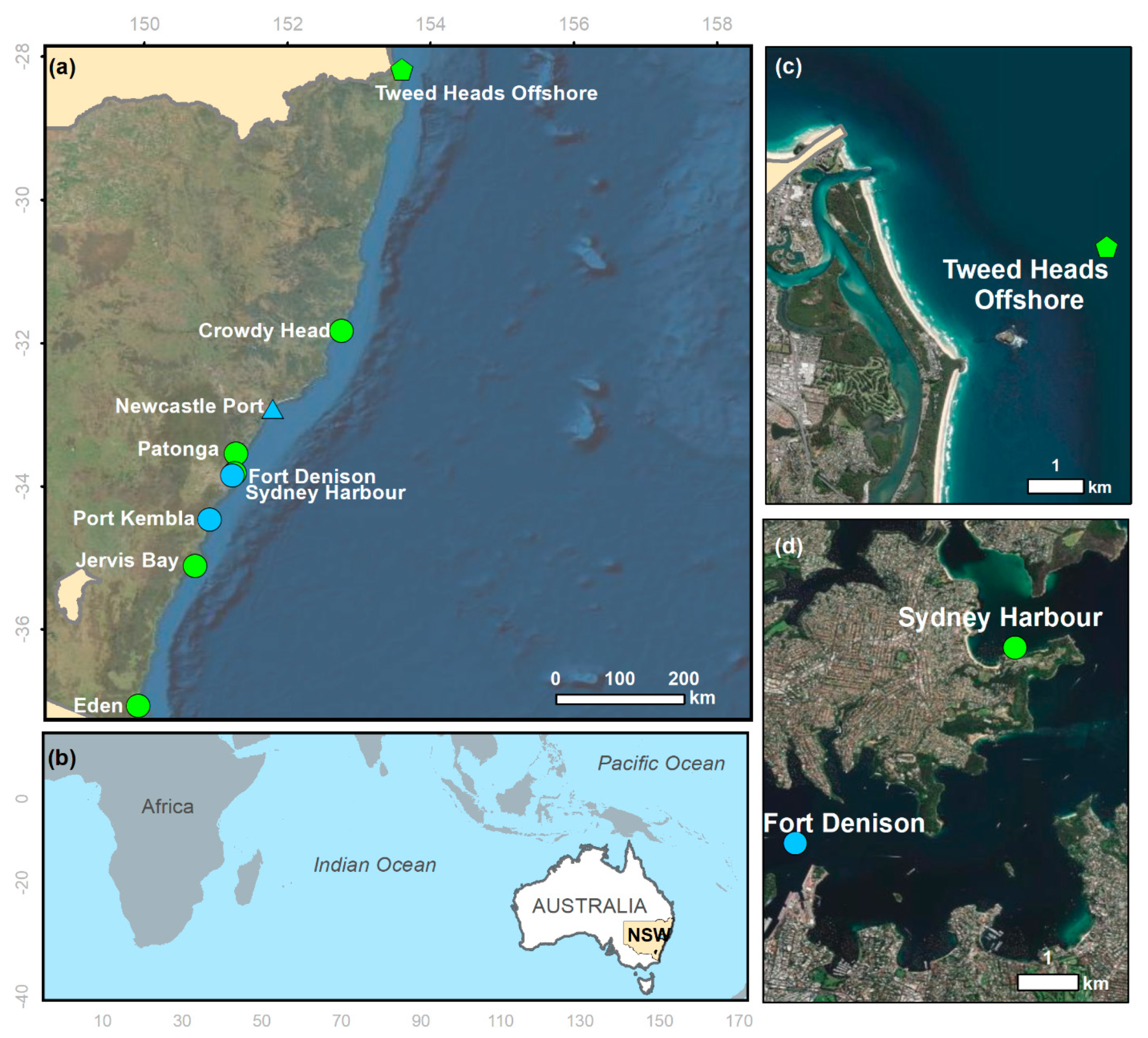
The NSW ocean tide network comprises 23 gauges: 18 gauges installed along the coast, four gauges installed offshore, and one gauge installed on an island. Herein, the analysis was limited to a subset of these gauges (Figure 1), as some are affected by rainfall, freshwater discharge, and/or seiches, while others have relatively short record lengths. Nine datasets were chosen based on the length of the records, the spatial coverage of the coast, and—whenever possible—the limited influence of flooding/freshwater discharge. The selected datasets comprised at least 25 years of water levels recorded with sampling frequencies of 15 or 60 min. One OOO dataset was included in the study to cover the northern part of the NSW coast to increase the spatial coverage. An ORE dataset with a record length > 50 years was also included to benefit from larger datasets. Of these datasets, six were provided by Manly Hydraulics Laboratory (MHL), and the remaining three datasets were obtained from the Australian Bureau of Meteorology (BoM) (Table 1).
The length of records is often a constraint for studies investigating the effects of climate processes with low frequencies or historical sea-level trends, since such studies require extended temporal coverage [30] (Figure 2). Additionally, most water level gauges along the north coast of NSW are ORE gauges owing to the geomorphology of the area; therefore, this region lacks OB gauges. Hence, ORE and OOO gauges were included in this study to increase the spatial coverage of the northern NSW coast.
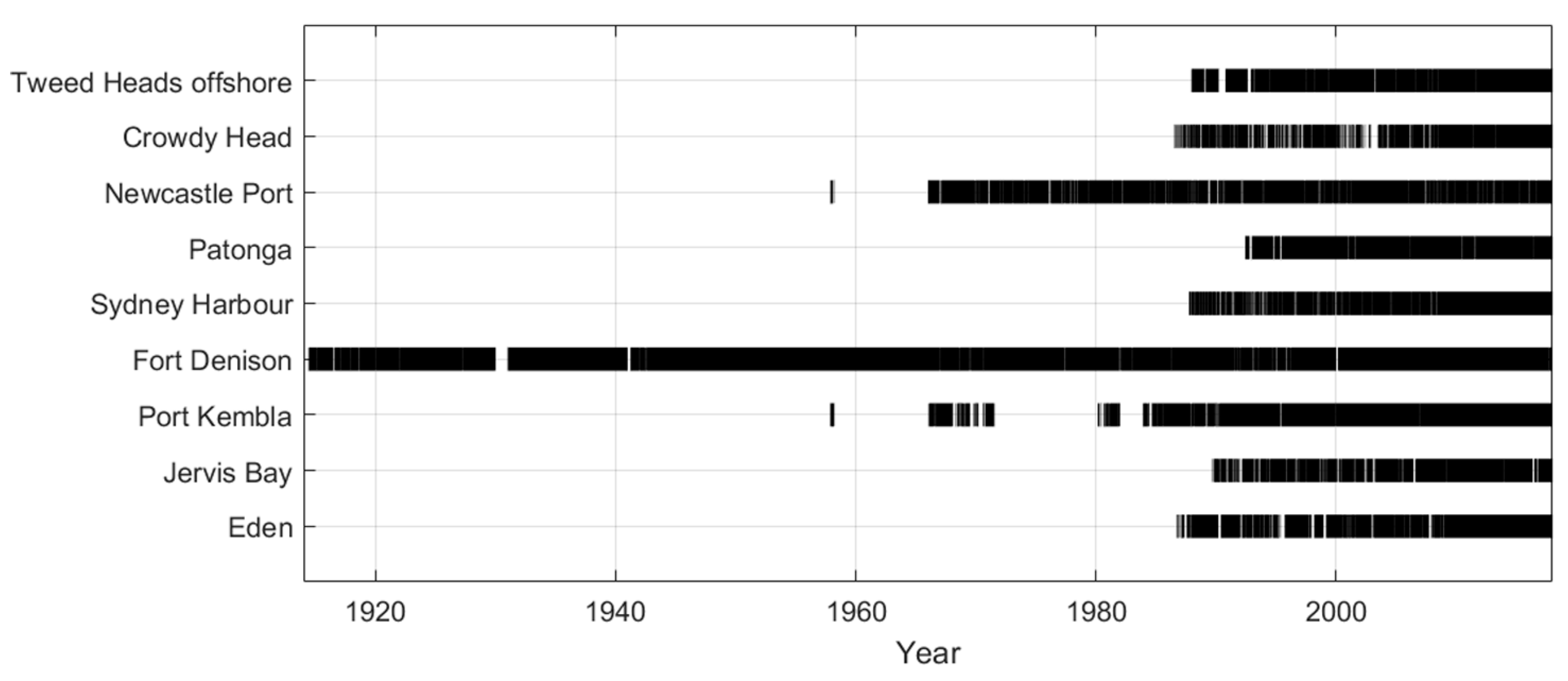
Ocean tide gauges in NSW have only been in full operation for approximately 30 years, with the exception of the three port gauges (Fort Denison, Newcastle Port, and Port Kembla) (Table 1). Fort Denison has been in operation since 1886, Newcastle Port since 1925, and Port Kembla since 1957 [31,32,33]. Despite these lengthy records, the Fort Denison record is considered less reliable before 1914, while Newcastle Port consists of gauges in three different sites (simply referred to as I, II, and III) within the harbour operating for different periods [31,34]. Considering this, the water level records of Fort Denison were taken from 1914, and those from Newcastle Port, from 1957. The Newcastle Port and Port Kembla gauges have long non-operation periods (at least five years), which are related to the periods immediately after the commencement of the operation of the two sites in 1957. In addition, Newcastle Port has an ORE gauge, and the removal of extreme events was performed to mitigate the influence of rainfall (see Section 3.2.2). To address these gaps, the early portions of the records were disregarded, and only data from 1969 (Newcastle Port) and 1983 (Port Kembla) onwards were used in this analysis. All remaining gauges have been operating since the mid–late 1980s.
3.2. Data Preparation
3.2.1. Seiches
Of the OB gauges, only the one in Crowdy Head is affected by seiches [15]. Seiching is a local process (related to harbour resonance); thus, it does not contribute to, nor is representative of, regional coastal or oceanographic processes. Seiches occur at specific ocean tide gauges along the NSW coast, with seiche periods usually between five minutes and two hours [35]. For Crowdy Head, MHL applies a low-pass filter to mitigate the effects of seiching, where one-minute data are recorded to provide information about the period and the amplitude of the seiche, in addition to the possible correlations with specific ocean conditions, which are then removed from the observed water levels [15]. Therefore, no further analyses were needed to prepare this dataset from the perspective of seiches at Crowdy Head.
3.2.2. Dataset Adjustments
Two sets of adjustments were made to the raw data in this study. These adjustments were made because the records were likely impacted by issues related to riverine floods and the offshore site (Tweed offshore), which lacks a surveyed datum. Therefore, four water level gauges and three additional ocean tide gauges were used for the flood-related peak and datum adjustment (Table 2). The methods used to account for the floods and the offshore datum are detailed below. The offshore datum was adjusted for an ORE gauge, which required flood-related analyses prior to the adjustment. Tweed Entrance South is the existing gauge at the mouth of the Tweed River, which has been in operation since 2014. The flood-related peak analysis was carried out at this gauge before adjusting the offshore dataset datum, which is detailed below.
Removing Flood-Related Peaks from ORE Records
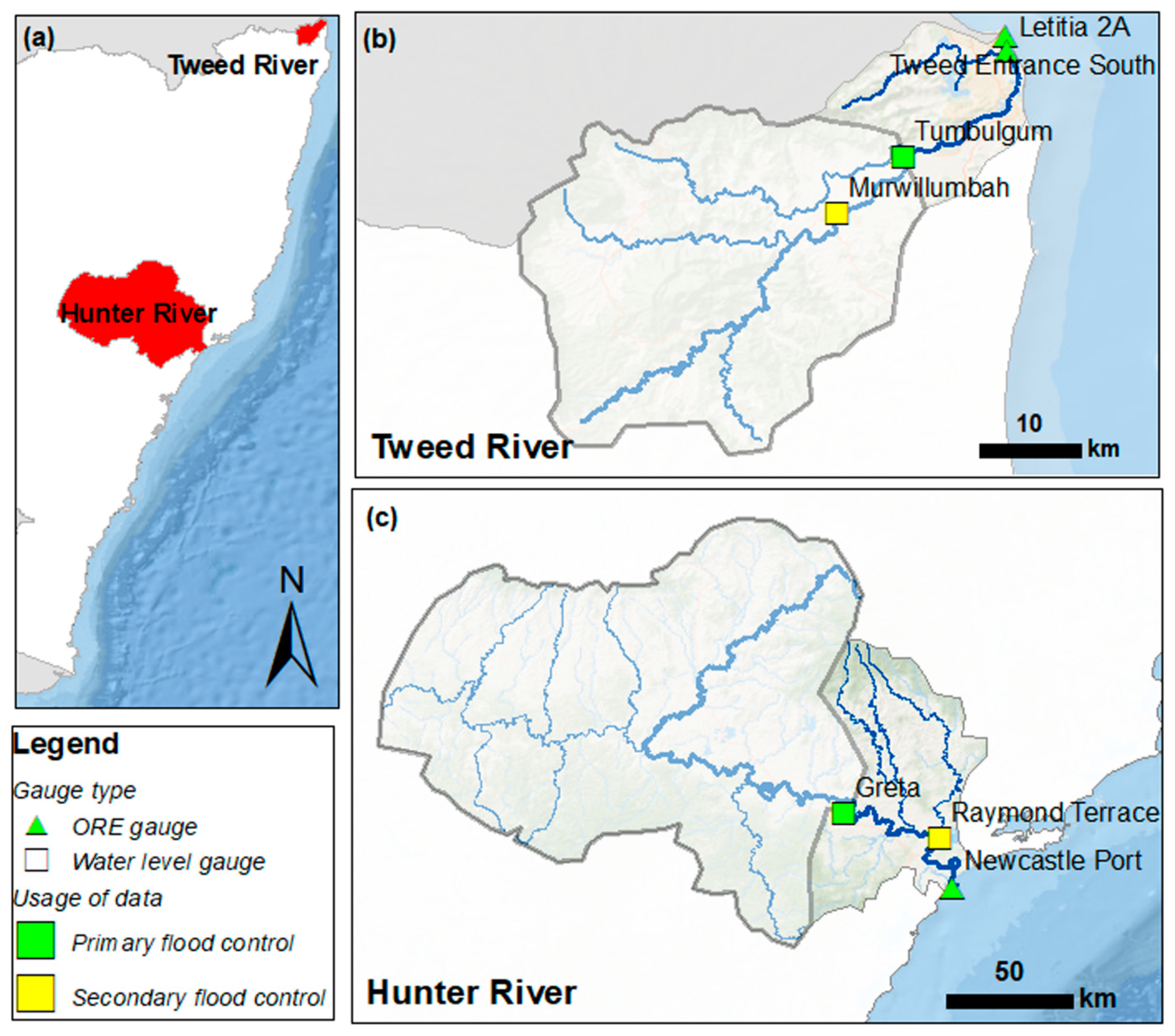
ORE gauges are susceptible to flood peaks caused by rainfall events within the river catchment, which flow downstream and reach the tide gauge. In these gauges, fresh rainfall inflows dominate the tidal signal during flood events, leading to an artificially raised water level. These events can potentially affect the harmonic analysis procedure; therefore, it is necessary to remove them prior to processing. This is common practice for tidal gauging sites in rivers, as the extreme values tend to skew the least-squares fit used to determine the harmonic constituents [6,15,36]. However, rainfall-related peaks are better observed on water level gauges located along rivers and not ocean tide gauges. Hence, the water level gauges were used as flood control gauges. For each catchment (Hunter and Tweed rivers), two water level gauges were selected as flood control gauges based on the visibility of the peaks, length of the records, and the catchment area (Figure 3). Periods associated with flood-related peaks were identified for the flood control gauges using a peak over threshold (POT). Then, the data corresponding to these periods were scrubbed from the two ORE gauges (Newcastle and Tweed Heads). As far as possible, the water level gauge records should have at least the same length as the ocean tide gauge records and present good coverage of the catchment area. Furthermore, the flood control gauges should ideally be located near the ocean tide gauge to account for the spatial distribution of the rainfall that is not across the catchment, i.e., the closer to the ORE, the more representative the water level gauge.
The sensitivity of the POT analysis to the choice of water level threshold was tested by observing the number of peaks that were above the arithmetic mean plus (i) 2 (95%), (ii) 2.5 (98.8%), and (iii) 3 (99.7%) standard deviations, based on the assumption that these water levels follow a Gaussian distribution. Option (i) and option (iii) were considered inadequate, as they returned a high and a low number of flood peaks, respectively, which did not match the historical records. However, option (ii) returned a realistic number of flooding events that could be verified using historical records in the region observed by the BoM; therefore, this option was chosen as the threshold in this study. Existing models can identify flood-related peaks effectively [37,38]. However, POT and the uniform tidal model were used to benefit from the comprehensive list of harmonic constituents included in Utide.
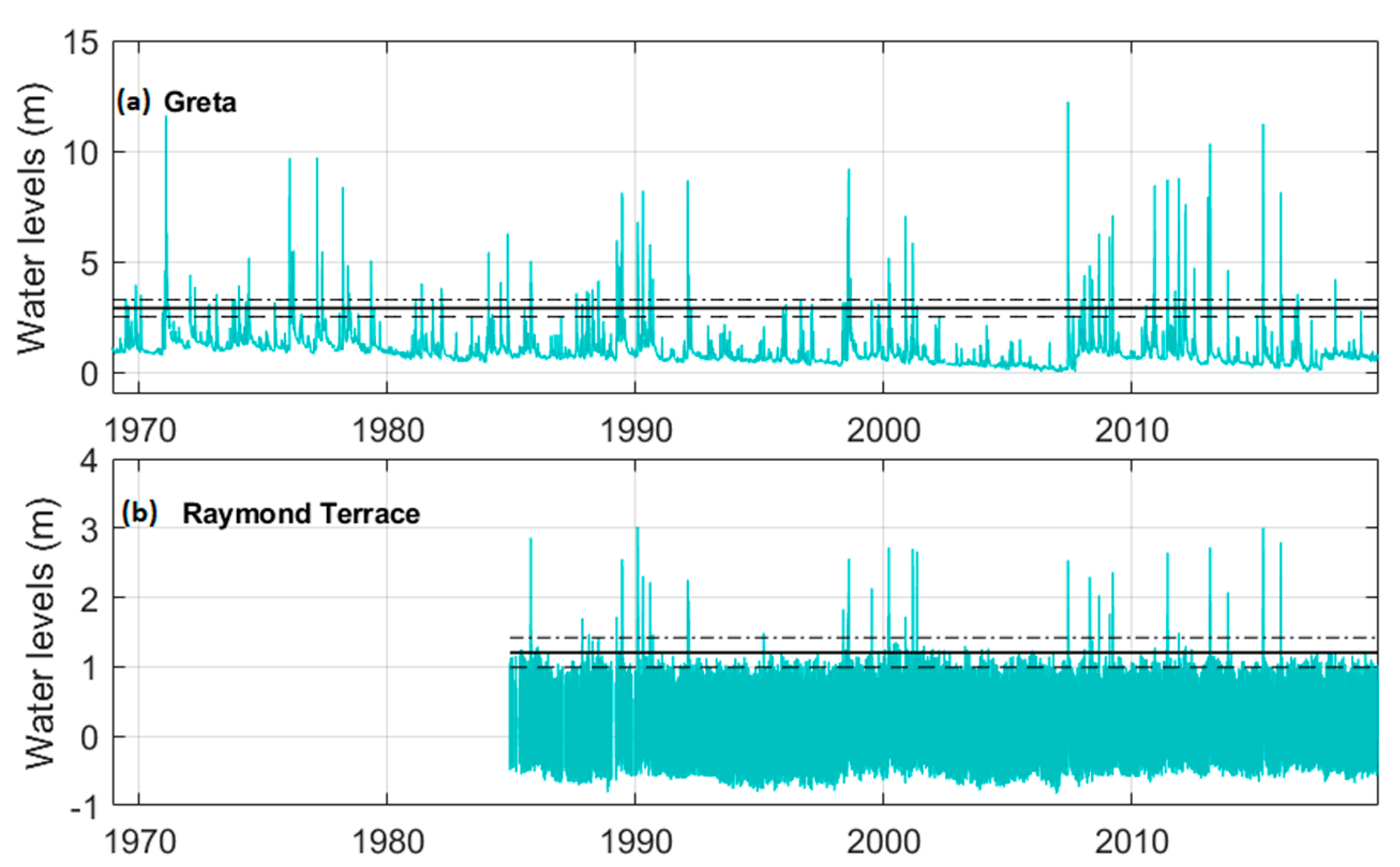
Greta was selected as the primary flood control gauge for Hunter River, and Raymond Terrace as the secondary control gauge (Figure 3). Raymond Terrace is a downstream gauge of Hunter River, approximately 30 km from Newcastle Port, and has been operating only since 1985. On the other hand, Greta has been in operation since 1969 and, even though it is approximately 80 km upstream of the river mouth, it has good coverage of the watershed, and the peaks in its records were clear (Figure 4). A threshold of 2.89 m was set for Greta and 1.2 m for Raymond Terrace, resulting from the mean plus 2.5 standard deviations (option ii) (Figure 4). The periods in which the recorded water levels in Greta surpassed the threshold were identified and verified in Raymond Terrace (where possible). The verification process also consisted of checking historical floods observed by the BoM during the identified periods for Greta. The data recorded during the periods in which water levels in Greta exceeded the threshold were then removed from the adjusted Newcastle Port dataset.
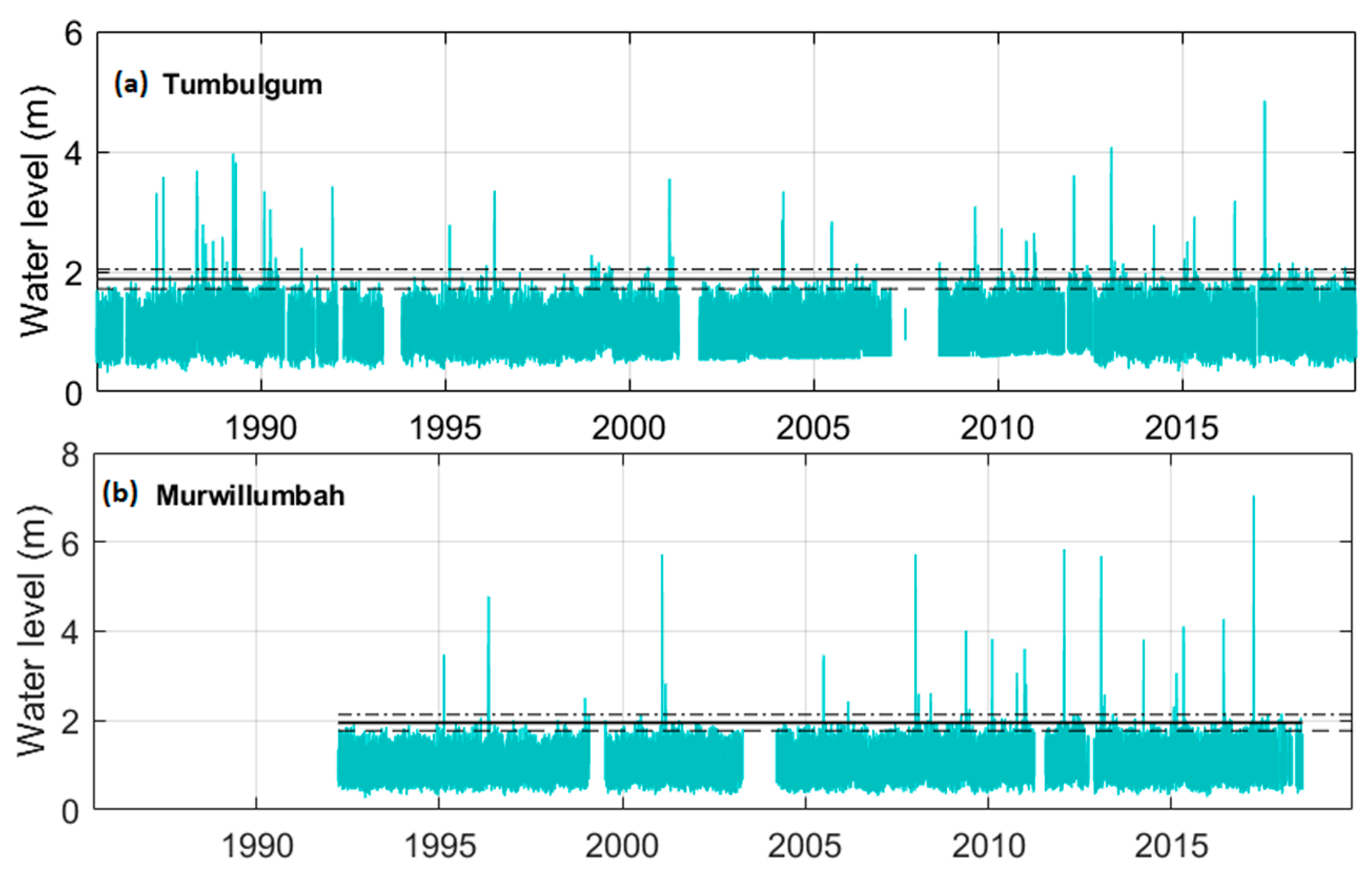
In a similar manner to the Hunter River, two water level gauges were selected for the Tweed River: a primary and a secondary flood control gauge. Tumbulgum, which has been in operation since 1985, was selected as the primary flood control gauge, and Murwillumbah was selected as the secondary flood control gauge (Figure 3). Thresholds of 1.88 m and 1.95 m were set for Tumbulgum and Murwillumbah, respectively, selected using the mean plus 2.5 standard deviations (option ii) (Figure 5). The periods in which the recorded water levels in Tumbulgum exceeded the threshold were identified and verified in Murwillumbah. Further analyses and verifications for the POT approach were similar to those previously described for the Hunter region.
Adjusting the OOO Dataset to a Fixed Datum
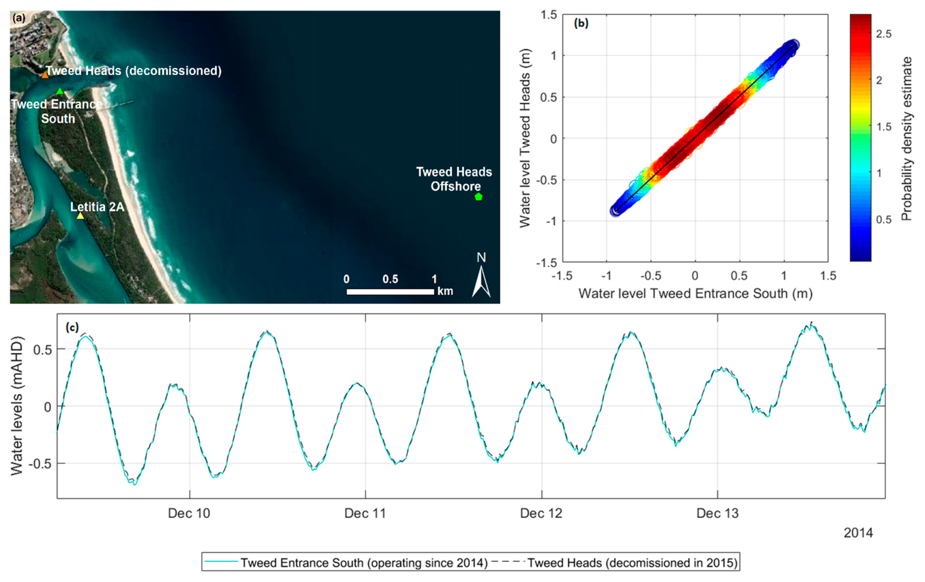
OOO gauges accurately capture tidal signals; however, they do not have a consistent datum [14]. These gauges are typically deployed every year and are referenced to the local mean sea level over the time of the deployment. This causes them to neglect the effects of significant climate processes on the water levels, such as the El Niño/Southern Oscillation (ENSO) and sea-level rise (SLR). To observe trends in tidal residuals, it is necessary to adjust these datasets to a fixed datum. The mouth of Tweed River is the closest area to the OOO gauge with existing AHD referenced gauges: Tweed Heads, which operated from 1987 to 2015; Tweed Entrance South, which has been in operation since 2014; and Letitia, which has been operating since 1987 (Figure 3). Tweed Heads and Tweed Entrance South are on opposite sides of the river mouth, about 200 m apart, and have overlaps in their data observation periods (i.e., 2014 to 2015), with highly correlated water levels during this time (R2 ≈ 0.99) (Figure 6). In addition, Tweed Entrance South was installed to replace the Tweed Heads gauge, and the two gauges were referenced to the same datum [36]. Therefore, these two records were combined into a single dataset, hereafter referred to as Tweed Entrance South, which was used to adjust the offshore record to the AHD. The data from Letitia 2A (Figure 3) was used to obtain water levels during the periods of missing data in Tweed Entrance South.
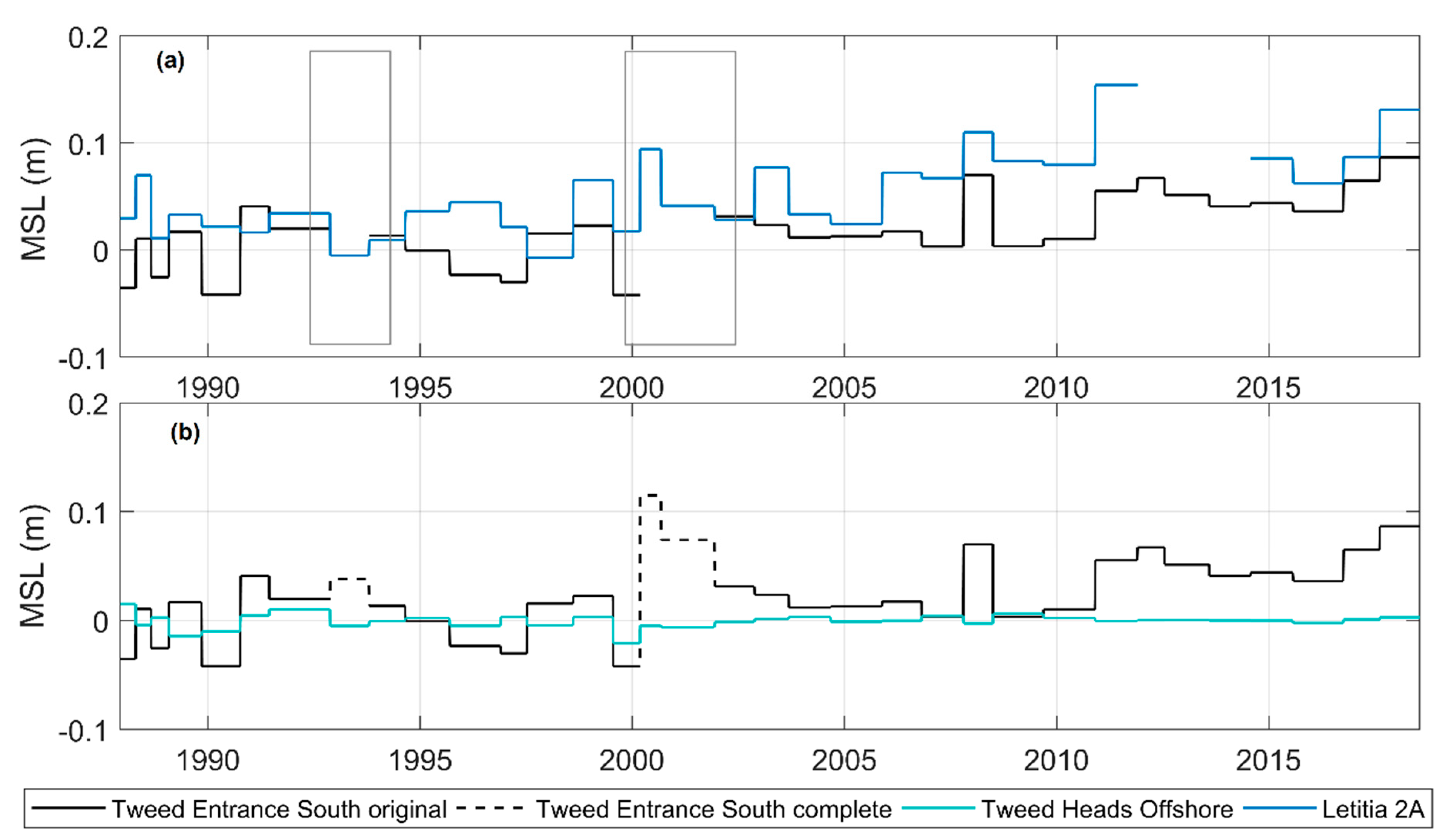
The OOO was adjusted to a fixed datum by observing the mean values for each deployment period in the Tweed Head Offshore and Tweed Entrance South gauges. The differences between these mean values for each deployment period were also obtained. Letitia 2A was used to account for the missing values in the Tweed Entrance South records owing to the proximity between the two gauges and the fact that—in general—the two records follow the same trend (Figure 7 and Figure 8). The relationship between the water levels at Letitia 2A and Tweed Entrance was also investigated, exhibiting a significant correlation with R2 ≈ 0.43 (95% confidence level) (Figure 7 and Figure 8). The resulting equation was then used to determine the missing values in the Tweed Entrance South dataset.
3.3. Calculation of the Tidal Residuals
3.3.1. Utide Model
The Utide model was used to predict tides for all datasets. Utide combines several known tidal analysis methods into one robust model that identifies the characteristics of tidal constituents and reconstructs the tidal signal (Codiga, 2011). The model was developed to handle datasets with gaps and/or irregular sampling frequencies, along with datasets with record lengths longer than two years, without compromising on the nodal/satellite corrections [25]. The tidal constituents can be either assigned or diagnosed in the model, which is advantageous because long and small amplitude constituents can be identified.
3.3.2. Timeseries of Tidal Residuals
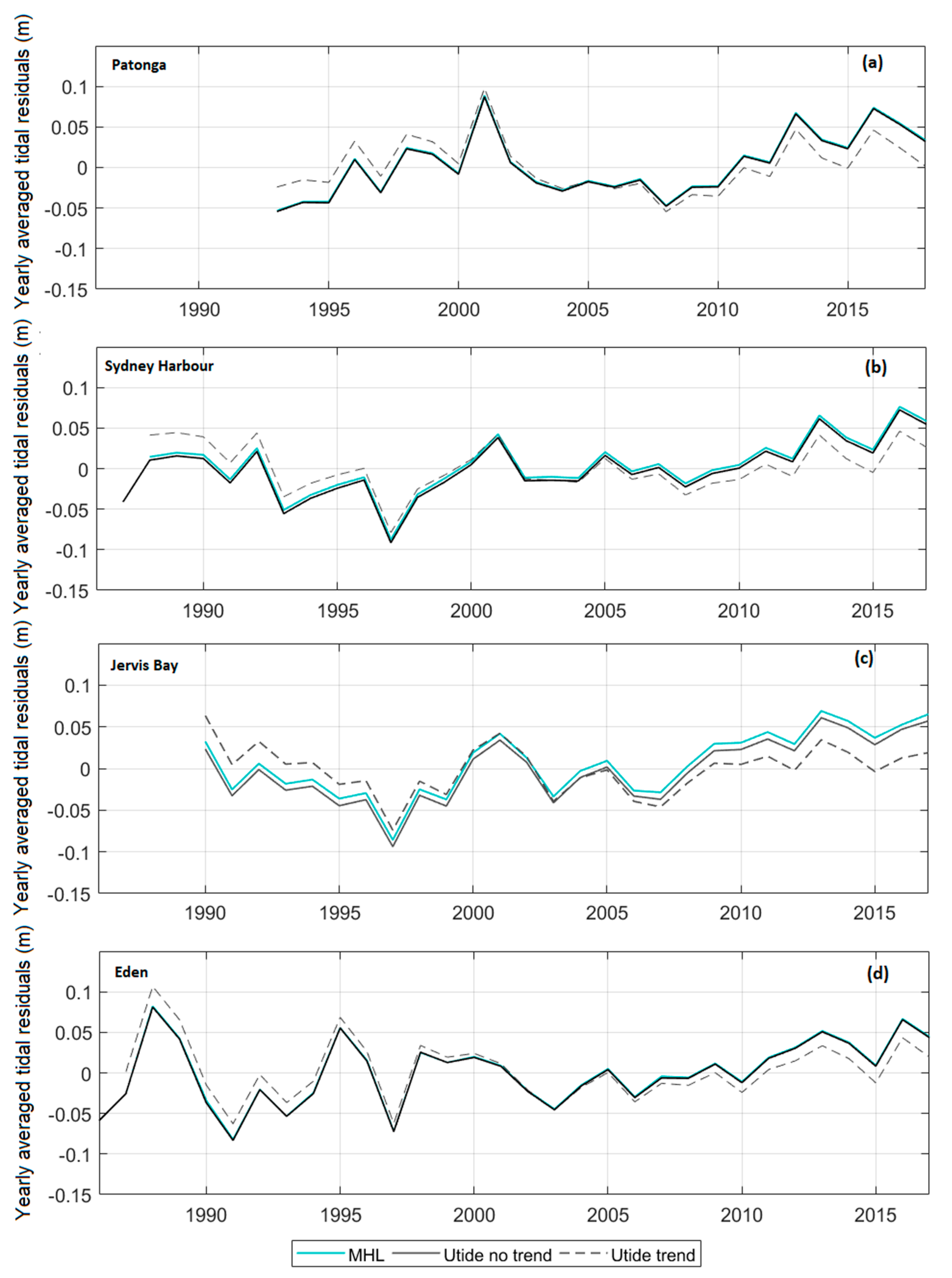
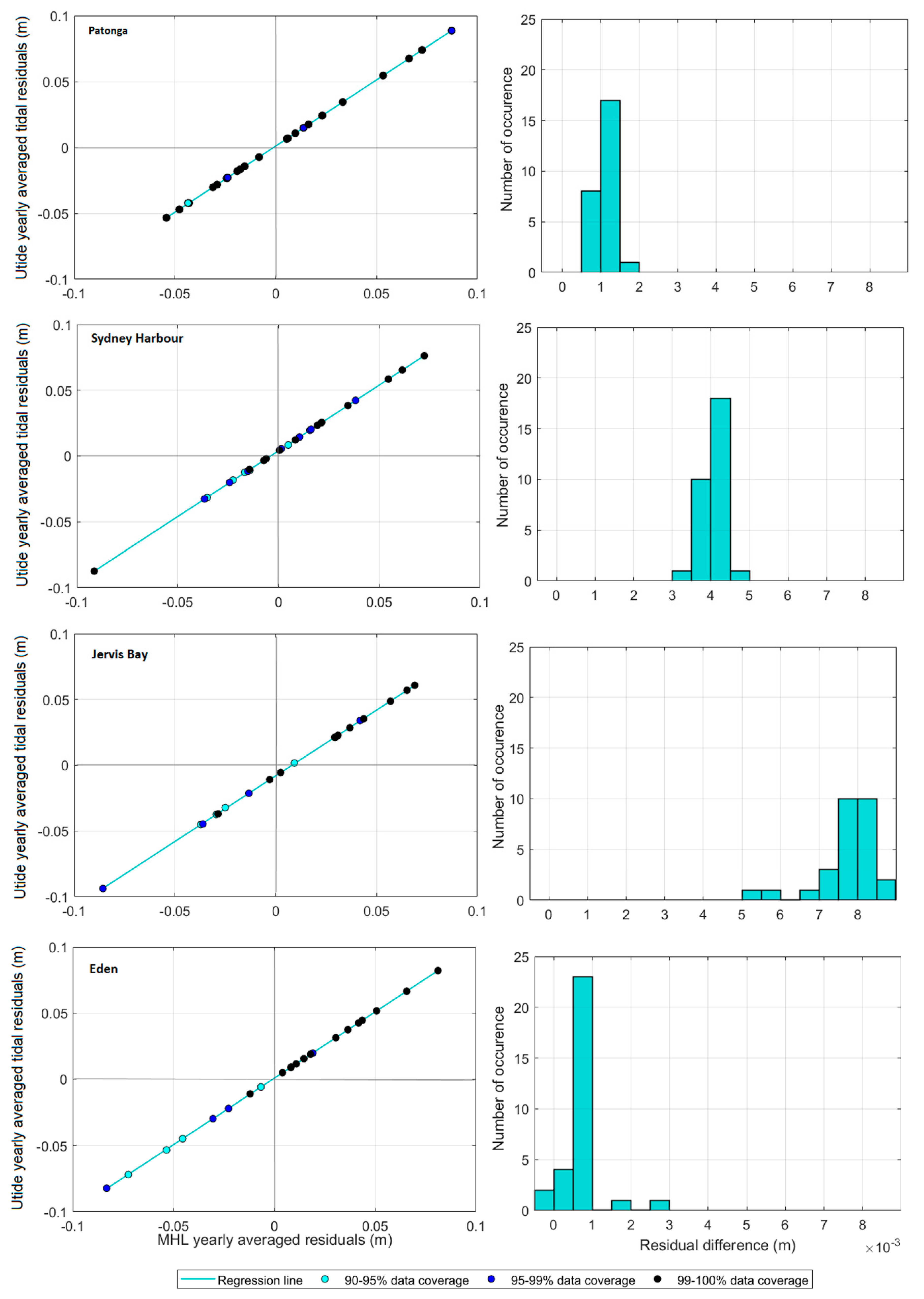
The Utide model was applied to all nine datasets to obtain the tidal residual time series. Overall, 68 constituents were calculated for all datasets and subsequently reconstructed into tidal predictions. To test the accuracy of the Utide model, it was run accounting (default) and not accounting (‘no trend’) for SLR. The accuracy of the predictions was verified by comparing the tidal residuals obtained from the model with the tidal residuals of four gauges (Eden, Jervis Bay, Sydney Harbour, and Patonga). The verification was based on observations of the correlations and a histogram of the differences between each pair of yearly averaged tidal residuals. The analysis showed that the ‘no trend’ option performed optimally, as the annual tidal residual means obtained from Utide were very similar to the annual means of the tidal residuals provided by MHL (Figure 9). MHL obtained the tidal residuals using the annual average method, which consists of averaging the constituents of a yearly analysis to generate longer predictions, thereby accounting for mean sea-level changes [39]. This method is based on the Foreman Versatile Tide, which, in combination with others methods (t_tide, r_t_tide and time-series handling), is incorporated in Utide [25]. MHL recommends this method considering that (1) the tide predictions should be performed using actual data rather than forecasted or modelled data, (2) historical tides should be analysed using data from the actual period under investigation, and (3) the constituents forecasted should be preferably determined by averaging their values of over 20 years. Although the method used here differs from the MHL method, the difference between the results is negligible (R2 ≥ 0.9998, p < 0.05), as shown in the obtained yearly averaged tidal residuals (Figure 9 and Figure 10). This can be explained by the fact that Utide considers the first and second MHL recommendations, and that every dataset used in this study is at least 25 years long (Figure 1), which is in accordance with the third MHL recommendation when forecasting constituents.
Overall, the tidal residuals from MHL were slightly larger than those obtained from Utide, under the ‘no trend’ scenario, with differences in the order of millimetres. Jervis Bay showed the largest difference, of approximately 1 cm (Figure 9). The results from the default scenario, ‘trend’, followed the same trend. However, there is an overestimation of the annual means until 2005, followed by an underestimation from 2005 onwards. Given that the tidal records used here are longer than the lunar nodal cycle (18.6 years), this automatically leads to accurate nodal/satellite corrections for the predicted tides and accounts for long-term sea-level rise. The tidal residuals provided by MHL serve as a baseline to the approach used, which increases the confidence in the results that will be further used in different analyses.
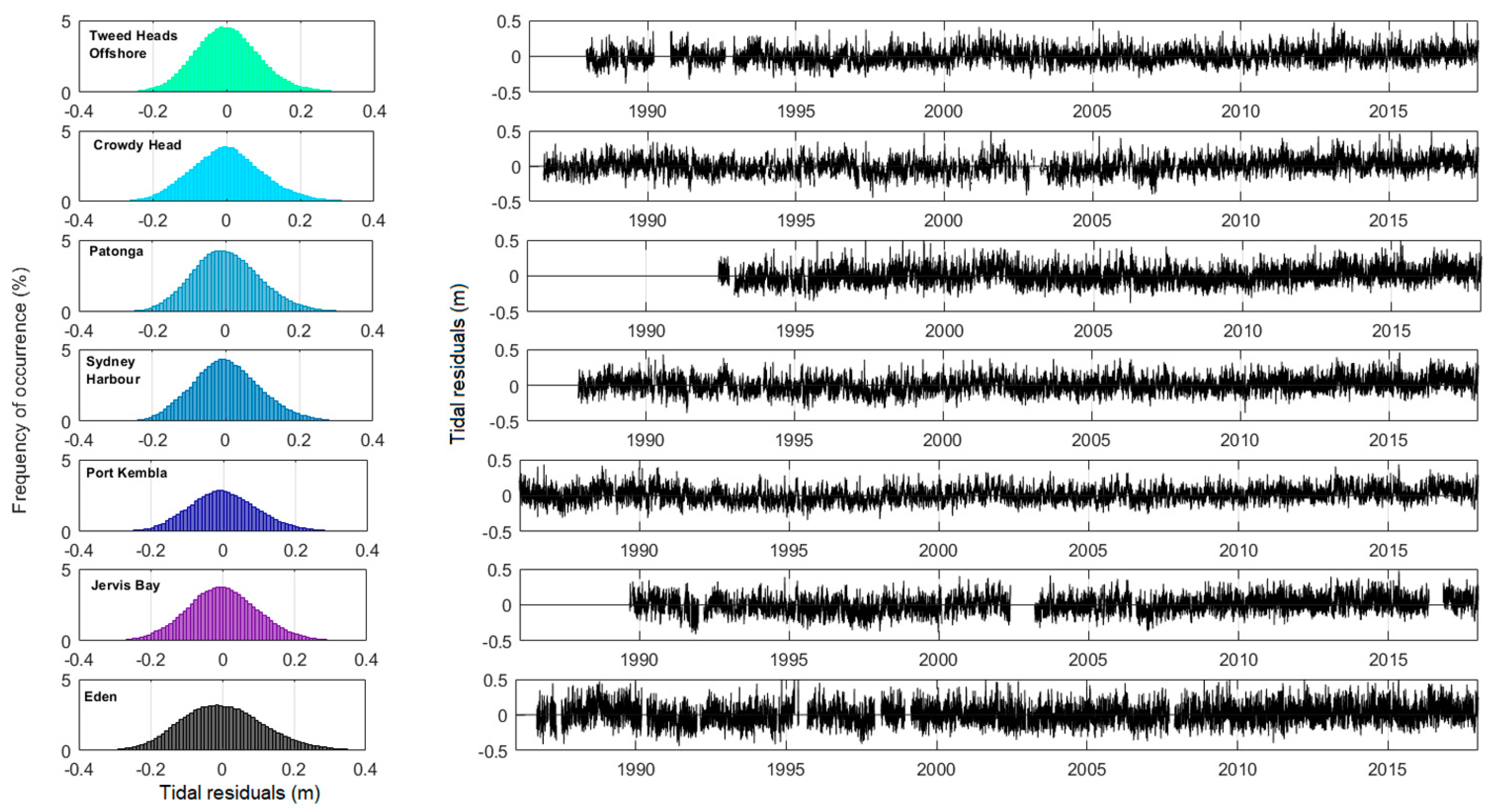
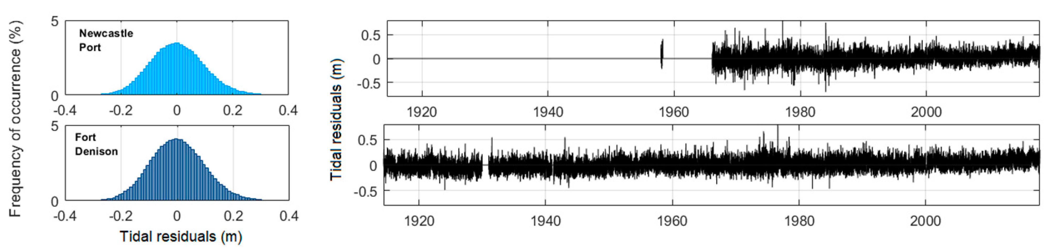
After comparing the obtained tidal residuals of the four gauges with the ones provided by MHL, the ‘no trend’ Utide approach was used for all the remaining gauges. The final tidal residuals are presented as continuous records and frequency distributions (Figure 11 and Figure 12). The tidal residuals are divided into two groups: (i) records with approximately 30 years of length and (ii) tidal residuals with at least 50 years of length (Fort Denison and Newcastle Port, respectively) (Figure 11 and Figure 12). The tidal residuals followed a normal distribution with amplitudes mostly varying from −0.4 to 0.4 m (Figure 11 and Figure 12). The harmonics used to predict the tides under the ‘no trend’ scenario are included in the Appendix A. In addition, time-series of original water levels, the predicted tides, and the tidal residuals during December 2017 were provided for each site (Figure A1, Figure A2, Figure A3, Figure A4, Figure A5, Figure A6, Figure A7, Figure A8 and Figure A9) in the Appendix A.
4. Applications of the Data
The compiled tidal residual datasets are extremely useful for coastal management, particularly in analysing extreme events. This information facilitates the accurate estimation of the frequency, magnitude, and duration of inundation at the synoptic, seasonal, interannual, and decadal scales using different techniques. Historical tidal residual datasets can be used to estimate future flooding scenarios and model future tidal levels (based on changes in MSL and large-scale synoptic conditions). This can help reduce the residential, commercial, infrastructural, and human losses resulting from flooding in the NSW coast and estuaries. The ability to estimate extreme water levels and inundation along the coast will improve the effectiveness of the response, adaptation, and mitigation of extreme events. The inclusion of the ORE gauge (Newcastle Port) increased the temporal scale, which facilitates long-term trend studies on NSW non-astronomical tidal residuals in addition to Fort Denison. The inclusion of the OOO dataset increased the spatial coverage of the NSW coast, especially in the north, where most gauges are influenced by freshwater and seiches. Next, a series of potential uses for these data are presented.
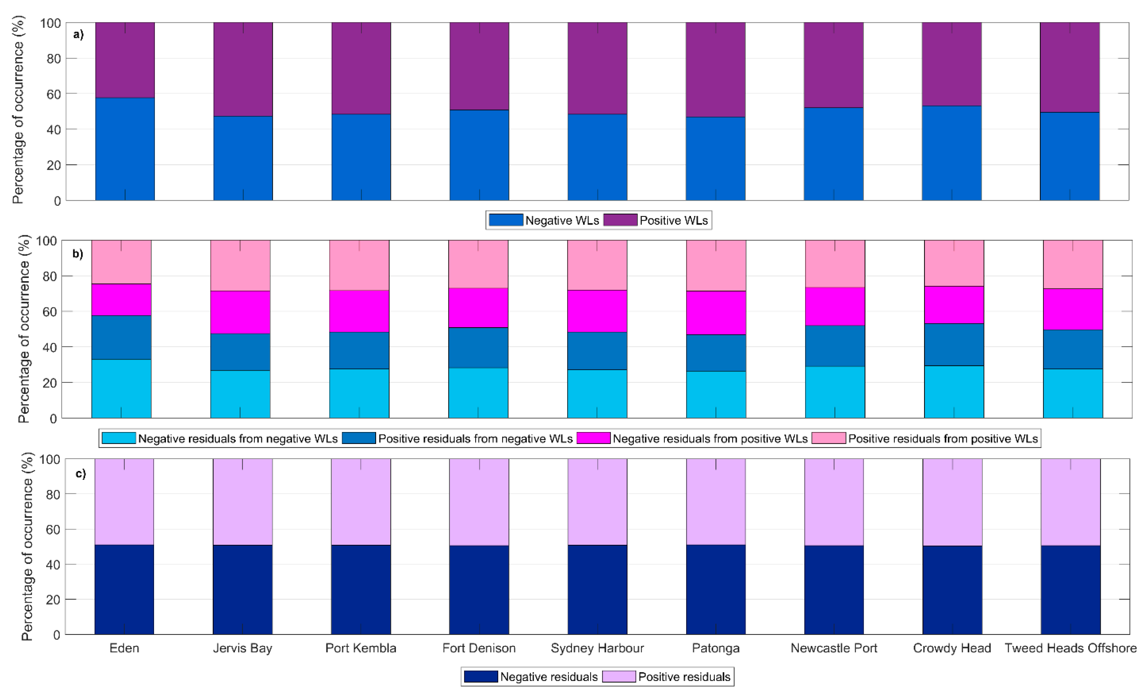
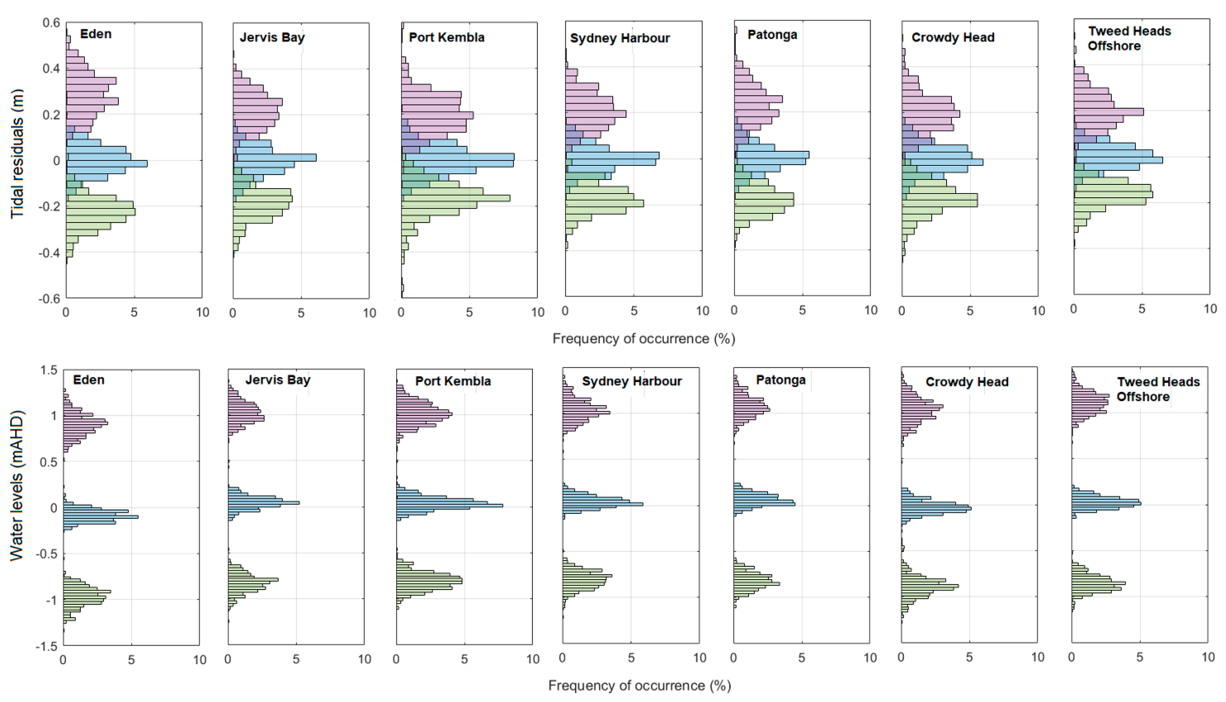
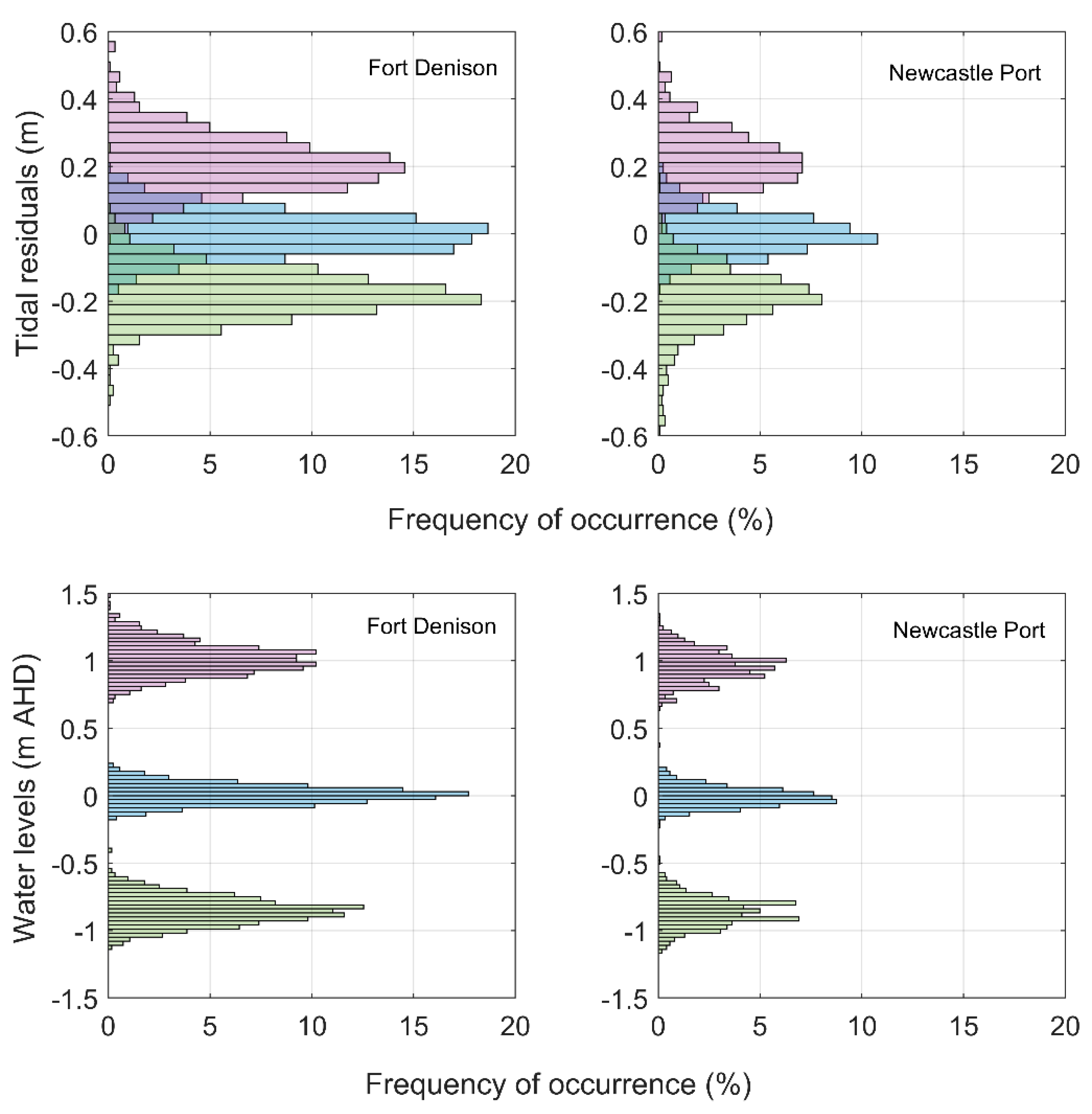
The tidal residuals presented herein can be used to understand the influences of a wide range of non-astronomic processes along the NSW coast. For example, it is possible to estimate the impacts of both tides and tidal residuals on increased water levels over spatial and temporal scales. Spatial scale studies can be conducted using datasets of approximately 30 years, while temporal scale studies can benefit from the two long records from Fort Denison and Newcastle Port. In addition, investigations of how tidal residuals vary according to tides can be carried out. This helps understand the likelihood of extreme events associated with large tides and tidal residuals. Figure 13 shows an example that takes the distribution of both tidal residuals and water levels into account, considering the relationship between positive and negative water levels and positive and negative tidal residuals 13. Here, it is observed that, on a spatial scale, tidal residuals are evenly distributed among all gauges: positive tidal residuals occurring as much as negative (approximately 50% positive and negative tidal residuals). The same was observed for water levels, except for Eden, where water levels were predominantly negative (Figure 13). It is also observed that although positive (negative) tidal residuals likely occur during positive (negative) water levels, at least 20% of positive (negative) tidal residuals occur during negative (positive) water levels (Figure 13).
The data can also support extreme analyses, which provide important information related to coastal inundation to assist coastal management. One way of using these data for extreme analyses can be done through observing the distribution of the maximum, mean, and minimum values (water levels and tidal residuals), as presented in Figure 14 and Figure 15. Except for Tweed Heads and Newcastle Port, means and minimum tidal residuals have higher frequencies and smaller standard deviations, while the maximum values have a larger variance and are less frequent (Figure 14 and Figure 15). On the other hand, maximum and minimum water levels are evenly distributed, with minimum values as frequent as maximum values (Figure 14 and Figure 15). In addition, an apparent shift in maximum water levels from the south to the north coast is observed, where larger water levels occur in the north (Figure 14). Again, an extreme analysis can be performed for the spatial (Figure 14) and temporal scales (Figure 15) and compared with existing studies on the magnitude of astronomic and non-astronomic processes along NSW [29]. Creating a comprehensive list of harmonics improves the understanding of tides, which is often limited in tidal prediction models. This limitation likely results in large standard deviations of data on the tides, increasing the astronomic effects on tidal residuals.
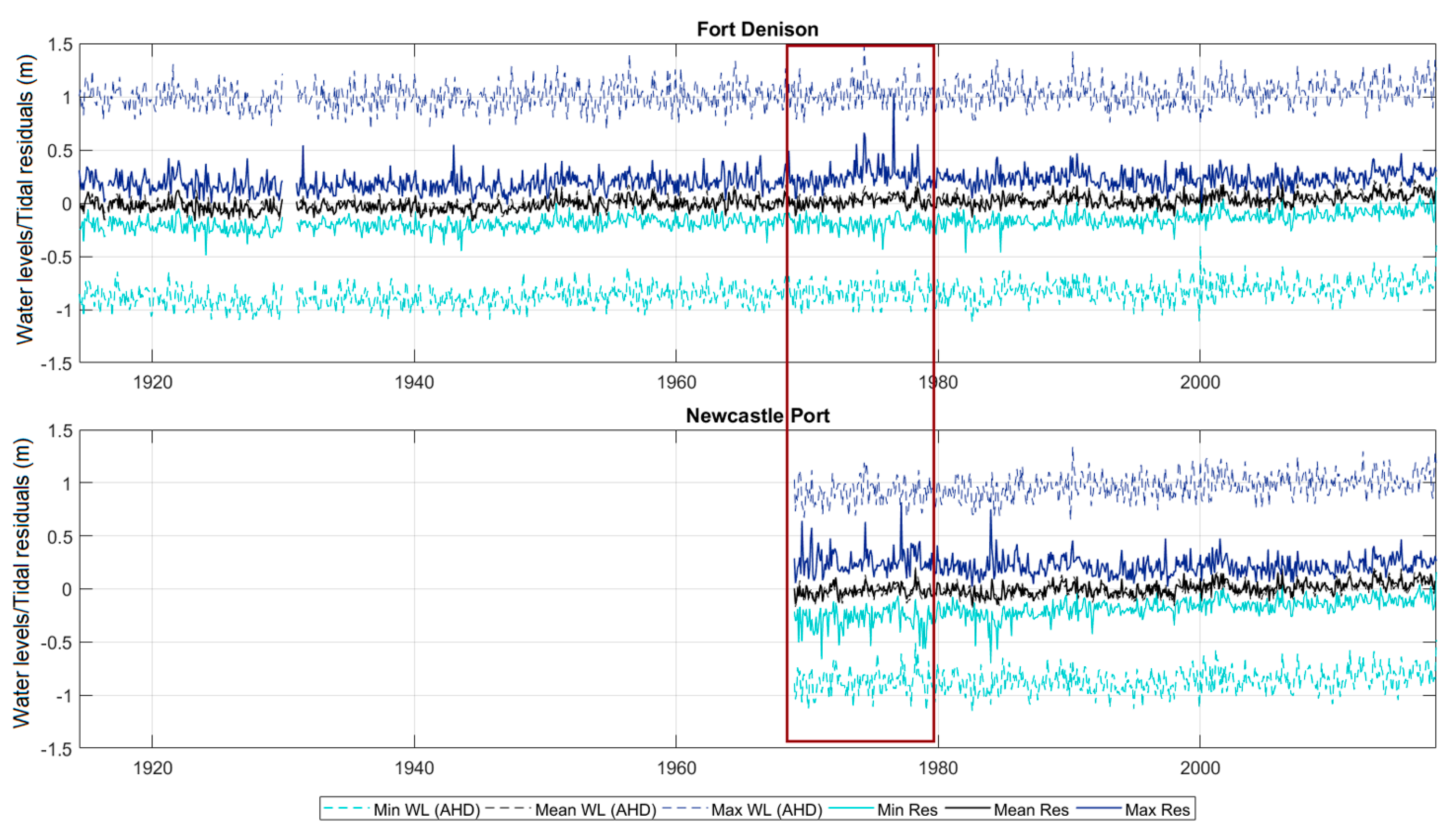
Small-scale, high-impact events can also be identified using these derived datasets. For example, the impact of the Sygna Storms in 1974 and the overall stormy period between 1970–1980 can be assessed (Figure 16). During this period, tidal residuals were amplified, likely because of extreme climate processes (e.g., frequent La Niña events) during that time or a higher occurrence of storms. For example, between 1974–1984, severe storms and east coast lows (ECLs) affected the NSW coast. This period was associated with significant damage in 1974 due to extreme events, including a flash flood in Sydney in April and an ECL in Newcastle in May [40].
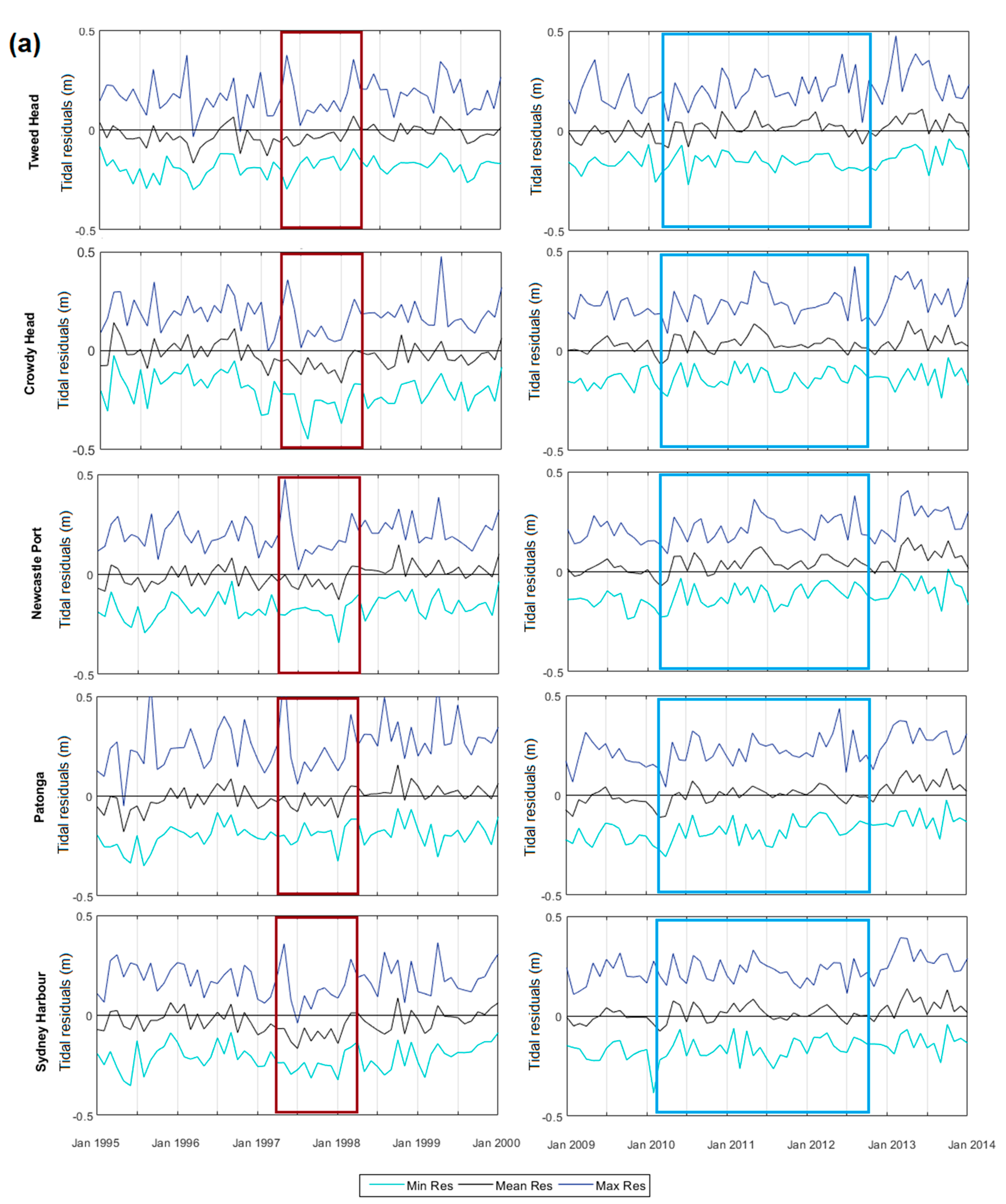
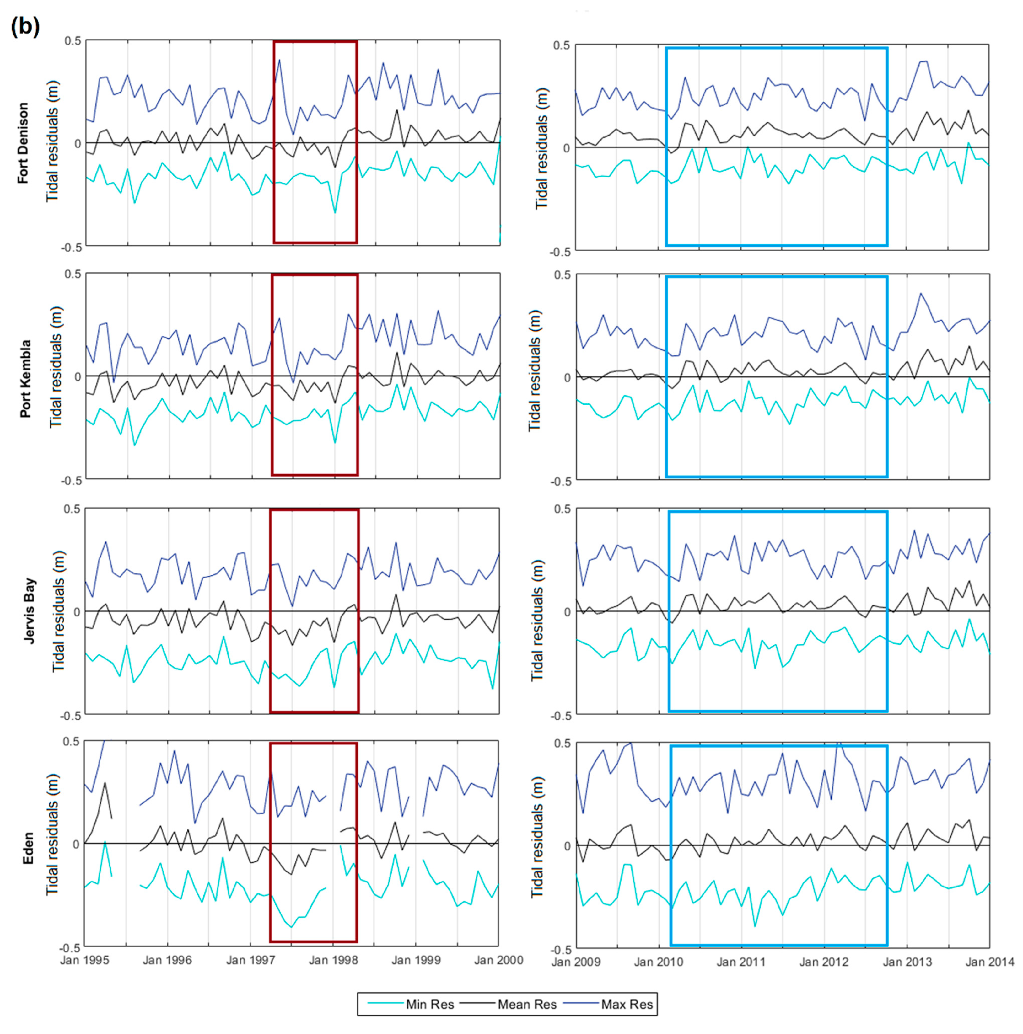
Tidal residuals can be affected by long-term climate modes (e.g., El Niño Southern Oscillation phases, El Niño, and La Niña) and short-term synoptic events (e.g., continental shelf waves, CSW, and ECLs). Thus, the tidal residual records can also be used in studies focusing on the impact of climate variability on NSW water levels. Figure 17 shows the distribution of monthly tidal residuals during the 1997–1998 El Niño and the 2010–2012 La Niña weather events to ascertain the impact of low-frequency cycles on water levels. This highlights how tidal residuals are likely to decrease during El Niño and increase during the La Niña phases, which is explained by the storminess variation resulting from ENSO.
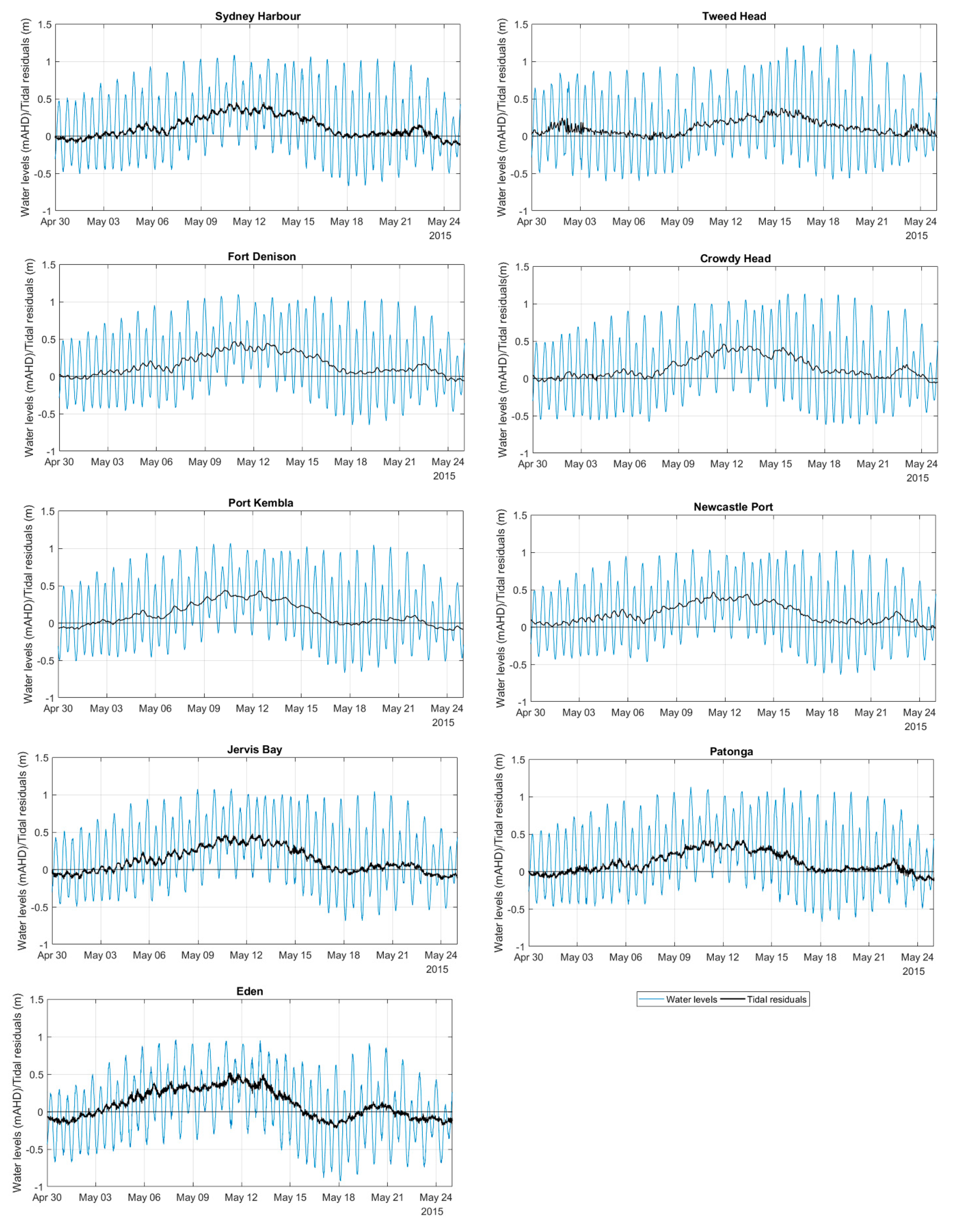
Examples of tidal residuals during continental shelf waves (CSWs) and ECLs are presented to highlight the impacts of common synoptic-scale events on tidal residuals. CSWs are common along the NSW coast, propagating northwards from Eden to Tweed Heads. CSWs are unidirectional waves with small amplitudes generated mainly within the Great Australian Bight, which are a result of wind stress and surface pressure gradients [41]. In May 2015, a CSW travelled along the coast and caused some degree of inundation [35]. The CSW had a period of approximately 12 days and caused elevated tidal residuals of approximately 0.3 m. The elevated water levels fully penetrated and caused extensive inundation in the surrounding areas of Lake Macquarie, a coastal lake where tides experience strong attenuation and do not penetrate fully. The effect of the CSW is shown in Figure 18, where consistency in duration and conservation of magnitude along the coast can be observed. The delay in the peaks of the wave from the southern to the northern gauges can also be observed, which is consistent with the conservation of the wave duration in south-to-north propagation.
ECLs are also common in NSW and cause extreme water levels that last from hours to a few days, along with intense rain and wind [42]. ECLs are maritime low-pressure systems formed in the mid-latitudes off continents’ east coast that last for a period of one to three days [42,43,44]. ECLs have a high frequency of occurrence (34% chance per year) and are considered to be one of the major weather hazards in NSW [45]. An example of tidal residuals caused by the passage of an ECL along the central coast of NSW is shown in Figure 19, where elevated water levels were observed for over three days.
5. Technical Validation
All of the ocean water levels used were referenced to the Australian Height Datum (AHD) before obtaining the tidal residuals. Furthermore, the OOO and the ORE datasets were carefully prepared to ensure the quality of the records by adjusting the datum and removing the flood-related records, as presented in the Methods section (Figure 4, Figure 5 and Figure 8).
The methods were carefully developed and compared with existing prediction models and tidal residual datasets of NSW ocean tide gauges. The tidal prediction model was verified through comparisons of the obtained and provided tidal residuals (MHL) for four gauges (Figure 9 and Figure 10). The set of harmonic constituents estimated using Utide is consistent with an existing study focused on the Fort Denison record [39]. MHL provided tidal residual records for four ocean tide gauges, including Patonga, Sydney Harbour, Eden, and Jervis Bay. However, the tidal residuals were (re)calculated for all datasets to ensure uniformity and facilitate comparisons among all datasets. Finally, the offshore dataset adjustment was carefully performed, using an AHD reference, and accounting for all deployment periods and missing data.
The quality assurance of these records was also investigated through buddy checking [46]. This process consisted of observing the differences in the tidal residuals of each pair of successive gauges. This approach facilitates better visualisation of possible instrumentation errors that were not captured through the observation of the original records and the tides. Abrupt shifts in the tidal residual differences were observed in several instances in Patonga and Sydney Harbour. During these instants, the tidal residual differences shifted from positive to negative (and vice-versa); after a while, they shifted back to their initial positions. This indicates potential instrument inaccuracies or errors during the data measurements, which could decrease the quality of future studies using these records [46,47,48]. Therefore, the data—in these instances—were erased from the Patonga and Sydney Harbour records, reducing the available data to 91.7% and 94.2%, respectively (Table 1).
Limitations
Pre-processing techniques can be complex to use when ascertaining ocean water levels, given the range of contributors involved. Tidal anomalies depend on tidal prediction tools that vary widely, and the operation of the ocean tide gauges and their location can also limit ocean water level investigations. In this study, the location of the gauges was a limitation, as few northern NSW ocean tide gauges were suitable for investigating the tidal residuals. For example, Newcastle Port is a gauge that has operated over a long period, but because it is an ORE gauge, the beginning of the record was limited to the knowledge of flood-related events. To identify and verify flood-related peaks, water level gauges near Newcastle Port were investigated, and a suitable gauge only began operating in 1969; therefore, records before that time were removed from the Newcastle Port dataset.
Funding
This research is funded by the University of Newcastle International Postgraduate Research Scholarship (UNIPRS) with the support of the Faculty for the Future from the Schlumburger Foundation. The Manly Hydraulics Laboratory tidal data is collected as part of the NSW Coastal Data Network Program for the Environment, Energy and Science Group in the NSW Department of Planning, Industry and Environment. Funding for this program comes from the NSW Climate Change Fund.
Institutional Review Board Statement
Not applicable.
Informed Consent Statement
Not applicable.
Data Availability Statement
All nine tidal residual datasets are available in NetCDF format for download (see data citation). The obtained harmonics for each gauge are available in Appendix A. The metadata includes the geographical coordinates and specific sources for input water levels.
Acknowledgments
We would like to express our gratitude to the Manly Hydraulics Laboratory team and Ben Hague, from the Bureau of Meteorology, for providing us with the time series of water levels along the NSW coast. This study was conducted on and used data collected from Indigenous land. The authors acknowledge the Traditional Owners of the lands: Bidwell, Yuin, Tharawal, Eora, Kuring-Gai, Biripi, and Budjalung. The authors also pay respects to the Indigenous elders of the past and present.
Conflicts of Interest
The authors declare no conflict of interest.
Appendix A

Table A1.
List of harmonic constituents obtained from Utide for three gauges in the southern NSW coast. The harmonics are sorted in ascending order of frequency of constituents. ‘H’ stands for amplitude in centimetres, ‘K’ stands for Greenwich phase lag in degrees.
Table A1.
List of harmonic constituents obtained from Utide for three gauges in the southern NSW coast. The harmonics are sorted in ascending order of frequency of constituents. ‘H’ stands for amplitude in centimetres, ‘K’ stands for Greenwich phase lag in degrees.
| Eden | Jervis Bay | Port Kembla | ||||||
|---|---|---|---|---|---|---|---|---|
| Harmonic | H(cm) | K (°) | Harmonic | H (cm) | K (°) | Harmonic | H (cm) | K (°) |
| SA | 3.410 | 146.12 | SA | 4.100 | 133.2 | SA | 4.030 | 138.31 |
| SSA | 1.900 | 154.68 | SSA | 2.220 | 145.59 | SSA | 1.830 | 143.62 |
| MSM | 0.194 | 317.34 | MSM | 0.352 | 347.33 | MSM | 0.278 | 305.23 |
| MM | 0.225 | 273.36 | MM | 0.107 | 317.82 | MM | 0.094 | 128.53 |
| MSF | 0.503 | 68.4 | MSF | 0.458 | 57.77 | MSF | 0.288 | 41.3 |
| MF | 0.480 | 196.32 | MF | 0.332 | 172.66 | MF | 0.406 | 160.14 |
| ALP1 | 0.136 | 197.89 | ALP1 | 0.123 | 205.3 | ALP1 | 0.129 | 194.67 |
| 2Q1 | 0.403 | 238.7 | 2Q1 | 0.363 | 236.74 | 2Q1 | 0.394 | 237 |
| SIG1 | 0.482 | 238.18 | SIG1 | 0.387 | 237.24 | SIG1 | 0.439 | 241.1 |
| Q1 | 2.560 | 267.24 | Q1 | 2.210 | 267.8 | Q1 | 2.440 | 272.41 |
| RHO1 | 0.480 | 268.51 | RHO1 | 0.421 | 275.58 | RHO1 | 0.457 | 276.09 |
| O1 | 11.100 | 287.26 | O1 | 9.710 | 287.44 | O1 | 10.500 | 294.59 |
| TAU1 | 0.085 | 245.41 | TAU1 | 0.052 | 238.86 | TAU1 | 0.107 | 252.63 |
| BET1 | 0.112 | 309.75 | BET1 | 0.061 | 326.8 | BET1 | 0.053 | 329.1 |
| NO1 | 0.824 | 302.4 | NO1 | 0.764 | 300.7 | NO1 | 0.769 | 312.63 |
| CHI1 | 0.156 | 302.52 | CHI1 | 0.106 | 314.53 | CHI1 | 0.128 | 309.48 |
| PI1 | 0.319 | 335.62 | PI1 | 0.277 | 339.56 | PI1 | 0.234 | 341.94 |
| P1 | 5.420 | 313.89 | P1 | 5.000 | 313.62 | P1 | 5.120 | 323.37 |
| S1 | 0.533 | 107.15 | S1 | 0.706 | 76.77 | S1 | 0.492 | 168.47 |
| K1 | 18.000 | 320.43 | K1 | 16.700 | 319.11 | K1 | 16.500 | 328.59 |
| PSI1 | 0.298 | 331.12 | PSI1 | 0.349 | 325.72 | PSI1 | 0.182 | 60.05 |
| PHI1 | 0.263 | 330.62 | PHI1 | 0.339 | 320.92 | PHI1 | 0.211 | 350.09 |
| THE1 | 0.180 | 339.21 | THE1 | 0.198 | 334.37 | THE1 | 0.181 | 343.08 |
| J1 | 0.998 | 343.62 | J1 | 1.010 | 342.68 | J1 | 1.000 | 347.67 |
| SO1 | 0.200 | 351.33 | SO1 | 0.179 | 353.1 | SO1 | 0.214 | 7.2 |
| OO1 | 0.721 | 19.14 | OO1 | 0.697 | 17.57 | OO1 | 0.621 | 24.61 |
| UPS1 | 0.112 | 42.72 | UPS1 | 0.111 | 44.2 | UPS1 | 0.109 | 50.64 |
| OQ2 | 0.226 | 249.56 | OQ2 | 0.233 | 249.67 | OQ2 | 0.241 | 253.56 |
| EPS2 | 0.565 | 274.05 | EPS2 | 0.564 | 273.86 | EPS2 | 0.605 | 274.19 |
| 2N2 | 1.950 | 279.01 | 2N2 | 2.010 | 278.8 | 2N2 | 1.960 | 280.61 |
| MU2 | 1.970 | 291.43 | MU2 | 2.050 | 291.16 | MU2 | 2.020 | 291.98 |
| N2 | 10.700 | 299.19 | N2 | 11.000 | 298.91 | N2 | 10.900 | 298.22 |
| NU2 | 2.000 | 300.4 | NU2 | 1.990 | 300.15 | NU2 | 1.980 | 298.74 |
| GAM2 | 0.252 | 327.58 | GAM2 | 0.244 | 310.46 | GAM2 | 0.132 | 301.27 |
| H1 | 0.464 | 197.71 | H1 | 0.493 | 191.92 | H1 | 0.345 | 183.84 |
| M2 | 46.800 | 308.74 | M2 | 49.200 | 306.68 | M2 | 48.800 | 307.52 |
| H2 | 0.269 | 201.16 | H2 | 0.228 | 196.77 | H2 | 0.257 | 192.63 |
| MKS2 | 0.174 | 45 | MKS2 | 0.137 | 37.43 | MKS2 | 0.155 | 44.13 |
| LDA2 | 0.548 | 294.53 | LDA2 | 0.567 | 292.25 | LDA2 | 0.535 | 288.71 |
| L2 | 1.280 | 308.32 | L2 | 1.340 | 307.08 | L2 | 1.320 | 306.52 |
| T2 | 0.698 | 348.07 | T2 | 0.718 | 341.99 | T2 | 0.770 | 341.94 |
| S2 | 10.300 | 321.21 | S2 | 11.400 | 320.24 | S2 | 11.900 | 320.63 |
| R2 | 0.157 | 254.18 | R2 | 0.169 | 269.82 | R2 | 0.150 | 273.46 |
| K2 | 3.140 | 308.23 | K2 | 3.470 | 308.17 | K2 | 3.560 | 309.24 |
| MSN2 | 0.174 | 176.65 | MSN2 | 0.197 | 176.77 | MSN2 | 0.179 | 185.34 |
| ETA2 | 0.172 | 298.6 | ETA2 | 0.216 | 295.99 | ETA2 | 0.228 | 297.63 |
| MO3 | 0.117 | 102.11 | MO3 | 0.093 | 83.79 | MO3 | 0.091 | 77.86 |
| M3 | 0.141 | 277.24 | M3 | 0.186 | 260.7 | M3 | 0.196 | 256.51 |
| SO3 | 0.036 | 197.65 | SO3 | 0.020 | 165.93 | SO3 | 0.012 | 131.39 |
| MK3 | 0.081 | 157.07 | MK3 | 0.046 | 130.99 | MK3 | 0.087 | 118.55 |
| SK3 | 0.194 | 19.83 | SK3 | 0.184 | 24.43 | SK3 | 0.162 | 26.64 |
| MN4 | 0.087 | 236.32 | MN4 | 0.084 | 232.76 | MN4 | 0.046 | 201.48 |
| M4 | 0.313 | 262.69 | M4 | 0.292 | 258.94 | M4 | 0.162 | 248.75 |
| SN4 | 0.021 | 225.91 | SN4 | 0.014 | 224.69 | SN4 | 0.013 | 229.35 |
| MS4 | 0.183 | 308.42 | MS4 | 0.149 | 312.05 | MS4 | 0.111 | 335.57 |
| MK4 | 0.067 | 288.28 | MK4 | 0.045 | 302.98 | MK4 | 0.021 | 19.85 |
| S4 | 0.036 | 80.97 | S4 | 0.045 | 71.23 | S4 | 0.034 | 77.97 |
| SK4 | 0.033 | 136.97 | SK4 | 0.028 | 143.97 | SK4 | 0.025 | 162.24 |
| 2MK5 | 0.046 | 25.63 | 2MK5 | 0.034 | 17.67 | 2MK5 | 0.022 | 288.76 |
| 2SK5 | 0.013 | 231.24 | 2SK5 | 0.019 | 195.67 | 2SK5 | 0.021 | 178.03 |
| 2MN6 | 0.026 | 220.81 | 2MN6 | 0.037 | 251.52 | 2MN6 | 0.055 | 230.07 |
| M6 | 0.107 | 269.31 | M6 | 0.134 | 278.25 | M6 | 0.145 | 265.53 |
| 2MS6 | 0.201 | 321.86 | 2MS6 | 0.219 | 321.24 | 2MS6 | 0.193 | 314.83 |
| 2MK6 | 0.066 | 334.81 | 2MK6 | 0.060 | 326.97 | 2MK6 | 0.059 | 334.51 |
| 2SM6 | 0.041 | 25.25 | 2SM6 | 0.043 | 15.76 | 2SM6 | 0.039 | 9.64 |
| MSK6 | 0.028 | 42.58 | MSK6 | 0.026 | 32.02 | MSK6 | 0.022 | 33.11 |
| 3MK7 | 0.003 | 13.29 | 3MK7 | 0.019 | 345.57 | 3MK7 | 0.004 | 326.79 |
| M8 | 0.011 | 135.19 | M8 | 0.005 | 47.34 | M8 | 0.006 | 101.03 |
Table A2.
List of harmonic constituents obtained from Utide for three gauges in the central coast of NSW. The harmonics are sorted in ascending order of frequency of constituents. ‘H’ stands for amplitude in centimetres, ‘K’ stands for Greenwich phase lag in degrees.
Table A2.
List of harmonic constituents obtained from Utide for three gauges in the central coast of NSW. The harmonics are sorted in ascending order of frequency of constituents. ‘H’ stands for amplitude in centimetres, ‘K’ stands for Greenwich phase lag in degrees.
| Fort Denison | Sydney Harbour | Patonga | ||||||
|---|---|---|---|---|---|---|---|---|
| Harmonic | H (cm) | K (°) | Harmonic | H (cm) | K (°) | Harmonic | H (cm) | K (°) |
| SA | 4.020 | 122.05 | SA | 3.850 | 140.13 | SA | 4.330 | 128.37 |
| SSA | 2.330 | 139.33 | SSA | 1.930 | 143.59 | SSA | 1.920 | 123.68 |
| MSM | 0.151 | 241.59 | MSM | 0.275 | 350.96 | MSM | 0.231 | 21.52 |
| MM | 0.102 | 177.05 | MM | 0.363 | 8.71 | MM | 0.255 | 353.33 |
| MSF | 0.115 | 183.49 | MSF | 0.351 | 64.74 | MSF | 0.305 | 87.6 |
| MF | 0.157 | 153.91 | MF | 0.270 | 182.68 | MF | 0.296 | 160.19 |
| ALP1 | 0.114 | 217.01 | ALP1 | 0.111 | 215.06 | ALP1 | 0.098 | 220.19 |
| 2Q1 | 0.377 | 243.54 | 2Q1 | 0.372 | 242.44 | 2Q1 | 0.387 | 241.85 |
| SIG1 | 0.420 | 249.32 | SIG1 | 0.412 | 245.93 | SIG1 | 0.390 | 250.94 |
| Q1 | 2.310 | 278.86 | Q1 | 2.290 | 279.32 | Q1 | 2.230 | 280.54 |
| RHO1 | 0.431 | 284.4 | RHO1 | 0.438 | 282.44 | RHO1 | 0.435 | 282.74 |
| O1 | 9.670 | 300.59 | O1 | 9.750 | 300.29 | O1 | 9.380 | 301.27 |
| TAU1 | 0.099 | 263.02 | TAU1 | 0.092 | 271.65 | TAU1 | 0.105 | 287.01 |
| BET1 | 0.052 | 307.93 | BET1 | 0.057 | 315.52 | BET1 | 0.057 | 299.14 |
| NO1 | 0.693 | 313.76 | NO1 | 0.678 | 314.83 | NO1 | 0.649 | 313.38 |
| CHI1 | 0.138 | 313.92 | CHI1 | 0.135 | 312.5 | CHI1 | 0.141 | 324.4 |
| PI1 | 0.285 | 333.07 | PI1 | 0.297 | 330.88 | PI1 | 0.298 | 338.86 |
| P1 | 4.410 | 326.28 | P1 | 4.430 | 325.06 | P1 | 4.340 | 324.58 |
| S1 | 0.508 | 166.42 | S1 | 0.577 | 198.64 | S1 | 0.317 | 168.1 |
| K1 | 14.900 | 329.44 | K1 | 15.000 | 328.9 | K1 | 14.700 | 328.31 |
| PSI1 | 0.158 | 217 | PSI1 | 0.186 | 220.57 | PSI1 | 0.280 | 247.17 |
| PHI1 | 0.126 | 310.93 | PHI1 | 0.161 | 313.9 | PHI1 | 0.178 | 302.98 |
| THE1 | 0.181 | 344.08 | THE1 | 0.156 | 346.45 | THE1 | 0.154 | 347.85 |
| J1 | 0.971 | 347.22 | J1 | 0.978 | 347.6 | J1 | 0.985 | 349.53 |
| SO1 | 0.160 | 6.98 | SO1 | 0.161 | 16.56 | SO1 | 0.142 | 11.08 |
| OO1 | 0.623 | 19.17 | OO1 | 0.614 | 18.04 | OO1 | 0.648 | 18.9 |
| UPS1 | 0.093 | 48.46 | UPS1 | 0.099 | 52.55 | UPS1 | 0.109 | 49.07 |
| OQ2 | 0.245 | 254.49 | OQ2 | 0.249 | 255.82 | OQ2 | 0.234 | 257.38 |
| EPS2 | 0.580 | 277.97 | EPS2 | 0.569 | 277.27 | EPS2 | 0.552 | 281.52 |
| 2N2 | 2.030 | 281.22 | 2N2 | 2.020 | 280.21 | 2N2 | 2.010 | 283.31 |
| MU2 | 2.110 | 291.84 | MU2 | 2.050 | 292.46 | MU2 | 2.040 | 297.12 |
| N2 | 11.400 | 299.53 | N2 | 11.200 | 297.98 | N2 | 11.300 | 301.47 |
| NU2 | 2.070 | 299.32 | NU2 | 2.030 | 297.32 | NU2 | 2.060 | 300.33 |
| GAM2 | 0.191 | 297.45 | GAM2 | 0.216 | 292.68 | GAM2 | 0.166 | 314.84 |
| H1 | 0.469 | 196.94 | H1 | 0.264 | 182.9 | H1 | 0.424 | 194.19 |
| M2 | 51.200 | 308.1 | M2 | 50.000 | 306.41 | M2 | 50.900 | 309.49 |
| H2 | 0.177 | 213.9 | H2 | 0.137 | 197.73 | H2 | 0.295 | 197.35 |
| MKS2 | 0.128 | 35.2 | MKS2 | 0.155 | 32.19 | MKS2 | 0.163 | 40.36 |
| LDA2 | 0.569 | 293.76 | LDA2 | 0.595 | 292.32 | LDA2 | 0.645 | 295.03 |
| L2 | 1.420 | 310.09 | L2 | 1.420 | 304.95 | L2 | 1.510 | 307.51 |
| T2 | 0.772 | 344.04 | T2 | 0.767 | 340.18 | T2 | 0.764 | 347.39 |
| S2 | 12.600 | 322.2 | S2 | 12.300 | 319.82 | S2 | 12.500 | 323.32 |
| R2 | 0.170 | 266.84 | R2 | 0.213 | 263.45 | R2 | 0.228 | 273.06 |
| K2 | 3.790 | 310.84 | K2 | 3.680 | 308.98 | K2 | 3.740 | 312.06 |
| MSN2 | 0.178 | 181 | MSN2 | 0.187 | 177.04 | MSN2 | 0.189 | 180.92 |
| ETA2 | 0.213 | 298.81 | ETA2 | 0.224 | 301.89 | ETA2 | 0.218 | 301.39 |
| MO3 | 0.047 | 115.32 | MO3 | 0.089 | 92.02 | MO3 | 0.116 | 83.06 |
| M3 | 0.237 | 254.66 | M3 | 0.232 | 252.16 | M3 | 0.247 | 255.9 |
| SO3 | 0.031 | 242.91 | SO3 | 0.040 | 179.19 | SO3 | 0.026 | 154.77 |
| MK3 | 0.078 | 199.95 | MK3 | 0.070 | 158 | MK3 | 0.064 | 136.77 |
| SK3 | 0.172 | 23.35 | SK3 | 0.144 | 25.49 | SK3 | 0.165 | 36.52 |
| MN4 | 0.117 | 236.91 | MN4 | 0.075 | 224.14 | MN4 | 0.067 | 261.93 |
| M4 | 0.376 | 253.71 | M4 | 0.250 | 244.26 | M4 | 0.302 | 282.3 |
| SN4 | 0.029 | 259.72 | SN4 | 0.014 | 206.14 | SN4 | 0.022 | 221.57 |
| MS4 | 0.168 | 297.54 | MS4 | 0.119 | 306.75 | MS4 | 0.151 | 329.07 |
| MK4 | 0.041 | 310.77 | MK4 | 0.034 | 295.66 | MK4 | 0.052 | 335.53 |
| S4 | 0.062 | 52.14 | S4 | 0.057 | 56.34 | S4 | 0.064 | 69.5 |
| SK4 | 0.028 | 169.47 | SK4 | 0.024 | 158.67 | SK4 | 0.019 | 182.03 |
| 2MK5 | 0.054 | 282.17 | 2MK5 | 0.015 | 307.36 | 2MK5 | 0.020 | 241.02 |
| 2SK5 | 0.018 | 186.64 | 2SK5 | 0.017 | 192.2 | 2SK5 | 0.023 | 210.66 |
| 2MN6 | 0.121 | 245.51 | 2MN6 | 0.056 | 230.79 | 2MN6 | 0.054 | 270.52 |
| M6 | 0.278 | 277.85 | M6 | 0.153 | 270.14 | M6 | 0.150 | 298.67 |
| 2MS6 | 0.248 | 317.28 | 2MS6 | 0.209 | 318.08 | 2MS6 | 0.218 | 338.5 |
| 2MK6 | 0.061 | 330.38 | 2MK6 | 0.069 | 329.74 | 2MK6 | 0.062 | 347.27 |
| 2SM6 | 0.024 | 337.51 | 2SM6 | 0.042 | 13.64 | 2SM6 | 0.045 | 16.18 |
| MSK6 | 0.023 | 35.56 | MSK6 | 0.026 | 26.42 | MSK6 | 0.029 | 36.11 |
| 3MK7 | 0.017 | 359.37 | 3MK7 | 0.006 | 67.7 | 3MK7 | 0.023 | 41.88 |
| M8 | 0.020 | 253.24 | M8 | 0.017 | 132.33 | M8 | 0.040 | 81.88 |
Table A3.
List of harmonic constituents obtained from Utide for three gauges in the northern coast of NSW. The harmonics are sorted in ascending order of frequency of constituents. ‘H’ stands for amplitude in centimetres, ‘K’ stands for Greenwich phase lag in degrees.
Table A3.
List of harmonic constituents obtained from Utide for three gauges in the northern coast of NSW. The harmonics are sorted in ascending order of frequency of constituents. ‘H’ stands for amplitude in centimetres, ‘K’ stands for Greenwich phase lag in degrees.
| Newcastle Port | Crowdy Head | Tweed Heads | ||||||
|---|---|---|---|---|---|---|---|---|
| Harmonic | H (cm) | K (°) | Harmonic | H (cm) | K (°) | Harmonic | H (cm) | K (°) |
| SA | 4.110 | 126.85 | SA | 5.540 | 149.39 | SA | 4.970 | 150.56 |
| SSA | 2.220 | 133.96 | SSA | 2.110 | 143.07 | SSA | 1.350 | 165.01 |
| MSM | 0.273 | 228.18 | MSM | 0.211 | 300.02 | MSM | 0.164 | 304.16 |
| MM | 0.093 | 199.08 | MM | 0.225 | 37.33 | MM | 0.485 | 67.68 |
| MSF | 0.398 | 107.32 | MSF | 0.309 | 106.8 | MSF | 0.247 | 136.54 |
| MF | 0.266 | 176.73 | MF | 0.214 | 184.68 | MF | 0.120 | 325.66 |
| ALP1 | 0.111 | 224.76 | ALP1 | 0.114 | 217.93 | ALP1 | 0.096 | 231.93 |
| 2Q1 | 0.339 | 244.67 | 2Q1 | 0.389 | 247.94 | 2Q1 | 0.342 | 262.86 |
| SIG1 | 0.375 | 248.9 | SIG1 | 0.411 | 251.65 | SIG1 | 0.362 | 270.19 |
| Q1 | 2.090 | 279.15 | Q1 | 2.450 | 283.62 | Q1 | 2.150 | 299.48 |
| RHO1 | 0.419 | 281.34 | RHO1 | 0.472 | 288.66 | RHO1 | 0.442 | 303.23 |
| O1 | 9.030 | 298.9 | O1 | 11.000 | 306.54 | O1 | 10.200 | 320.41 |
| TAU1 | 0.066 | 306.81 | TAU1 | 0.092 | 257.59 | TAU1 | 0.079 | 340 |
| BET1 | 0.068 | 306.78 | BET1 | 0.052 | 328.05 | BET1 | 0.097 | 344.37 |
| NO1 | 0.707 | 310.38 | NO1 | 0.828 | 320.88 | NO1 | 0.781 | 334.37 |
| CHI1 | 0.142 | 314.4 | CHI1 | 0.178 | 319.83 | CHI1 | 0.164 | 344.05 |
| PI1 | 0.337 | 345.44 | PI1 | 0.241 | 338.24 | PI1 | 0.298 | 7.99 |
| P1 | 4.670 | 320.64 | P1 | 5.140 | 333.57 | P1 | 5.420 | 344.03 |
| S1 | 0.608 | 80.76 | S1 | 0.937 | 172.89 | S1 | 0.382 | 156.56 |
| K1 | 16.000 | 327.22 | K1 | 17.200 | 338.24 | K1 | 18.100 | 350.85 |
| PSI1 | 0.379 | 304.91 | PSI1 | 0.138 | 186.33 | PSI1 | 0.045 | 260.68 |
| PHI1 | 0.314 | 314.56 | PHI1 | 0.183 | 347.06 | PHI1 | 0.260 | 10.84 |
| THE1 | 0.206 | 335.85 | THE1 | 0.180 | 354.08 | THE1 | 0.237 | 1.28 |
| J1 | 1.050 | 349.61 | J1 | 1.100 | 355.88 | J1 | 1.140 | 9.11 |
| SO1 | 0.205 | 6.2 | SO1 | 0.157 | 11.24 | SO1 | 0.211 | 18.34 |
| OO1 | 0.692 | 24.34 | OO1 | 0.680 | 26.27 | OO1 | 0.752 | 40.94 |
| UPS1 | 0.105 | 52.29 | UPS1 | 0.123 | 62.02 | UPS1 | 0.128 | 66.24 |
| OQ2 | 0.233 | 260.4 | OQ2 | 0.257 | 255.28 | OQ2 | 0.253 | 258.31 |
| EPS2 | 0.549 | 279.18 | EPS2 | 0.607 | 279.3 | EPS2 | 0.554 | 276.35 |
| 2N2 | 1.960 | 283.18 | 2N2 | 2.050 | 280.39 | 2N2 | 1.950 | 279.1 |
| MU2 | 2.010 | 294.16 | MU2 | 2.090 | 291.46 | MU2 | 2.000 | 287.77 |
| N2 | 10.900 | 301.22 | N2 | 11.300 | 295.85 | N2 | 11.400 | 291.26 |
| NU2 | 2.000 | 300.89 | NU2 | 2.080 | 295.68 | NU2 | 2.100 | 290.53 |
| GAM2 | 0.089 | 298.49 | GAM2 | 0.201 | 308.63 | GAM2 | 0.209 | 287.65 |
| H1 | 0.432 | 224.05 | H1 | 0.427 | 198.85 | H1 | 0.267 | 230.38 |
| M2 | 49.600 | 309.33 | M2 | 52.500 | 304.27 | M2 | 53.300 | 300.02 |
| H2 | 0.260 | 236.93 | H2 | 0.214 | 222.76 | H2 | 0.235 | 247.94 |
| MKS2 | 0.167 | 85.48 | MKS2 | 0.119 | 18.17 | MKS2 | 0.209 | 77.79 |
| LDA2 | 0.555 | 299.1 | LDA2 | 0.579 | 294.05 | LDA2 | 0.519 | 295.84 |
| L2 | 1.370 | 312.76 | L2 | 1.420 | 304.04 | L2 | 1.470 | 301.28 |
| T2 | 0.707 | 347.08 | T2 | 0.866 | 338.44 | T2 | 0.955 | 322.68 |
| S2 | 12.400 | 323.31 | S2 | 13.800 | 317.09 | S2 | 15.500 | 309.54 |
| R2 | 0.173 | 276.81 | R2 | 0.212 | 265.3 | R2 | 0.253 | 268.56 |
| K2 | 3.700 | 311.64 | K2 | 4.130 | 306.77 | K2 | 4.580 | 300.89 |
| MSN2 | 0.159 | 194.31 | MSN2 | 0.149 | 184.65 | MSN2 | 0.125 | 192.62 |
| ETA2 | 0.239 | 288.64 | ETA2 | 0.252 | 303.28 | ETA2 | 0.299 | 298.03 |
| MO3 | 0.043 | 167.55 | MO3 | 0.033 | 46.91 | MO3 | 0.014 | 356.27 |
| M3 | 0.248 | 254.02 | M3 | 0.316 | 239.17 | M3 | 0.560 | 227.07 |
| SO3 | 0.020 | 309.42 | SO3 | 0.010 | 135.29 | SO3 | 0.037 | 91.71 |
| MK3 | 0.041 | 254.14 | MK3 | 0.051 | 169.55 | MK3 | 0.054 | 180.32 |
| SK3 | 0.144 | 23.48 | SK3 | 0.087 | 43.7 | SK3 | 0.067 | 155.51 |
| MN4 | 0.118 | 291.1 | MN4 | 0.026 | 211.7 | MN4 | 0.026 | 111.77 |
| M4 | 0.419 | 288.17 | M4 | 0.162 | 242.83 | M4 | 0.156 | 206.54 |
| SN4 | 0.011 | 20.58 | SN4 | 0.001 | 144.28 | SN4 | 0.006 | 162.38 |
| MS4 | 0.236 | 327.02 | MS4 | 0.053 | 329.99 | MS4 | 0.040 | 149.75 |
| MK4 | 0.062 | 334.89 | MK4 | 0.024 | 4.47 | MK4 | 0.021 | 110.8 |
| S4 | 0.101 | 57.75 | S4 | 0.091 | 38.52 | S4 | 0.120 | 49.78 |
| SK4 | 0.014 | 259.1 | SK4 | 0.015 | 230.9 | SK4 | 0.021 | 255.59 |
| 2MK5 | 0.089 | 301.72 | 2MK5 | 0.029 | 243.17 | 2MK5 | 0.011 | 303.44 |
| 2SK5 | 0.029 | 174.76 | 2SK5 | 0.033 | 159.26 | 2SK5 | 0.054 | 154.39 |
| 2MN6 | 0.162 | 286.2 | 2MN6 | 0.040 | 260.72 | 2MN6 | 0.063 | 294.77 |
| M6 | 0.374 | 302.45 | M6 | 0.076 | 278.95 | M6 | 0.083 | 329.72 |
| 2MS6 | 0.325 | 329.25 | 2MS6 | 0.078 | 307.6 | 2MS6 | 0.082 | 211.8 |
| 2MK6 | 0.106 | 330.25 | 2MK6 | 0.018 | 308.44 | 2MK6 | 0.032 | 213.55 |
| 2SM6 | 0.037 | 359.87 | 2SM6 | 0.016 | 348.6 | 2SM6 | 0.039 | 282.17 |
| MSK6 | 0.027 | 13.9 | MSK6 | 0.007 | 357.37 | MSK6 | 0.024 | 285.03 |
| 3MK7 | 0.026 | 184.14 | 3MK7 | 0.001 | 41.76 | 3MK7 | 0.013 | 79.07 |
| M8 | 0.047 | 263.64 | M8 | 0.001 | 346.67 | M8 | 0.016 | 34.32 |
Figure A1.
Time-series of observed sea water levels in Tweed Heads Offshore during December 2017. The blue line indicates the observed water level. The green line indicates the predicted tide using Utide. The black line represents the obtained tidal residuals.
Figure A1.
Time-series of observed sea water levels in Tweed Heads Offshore during December 2017. The blue line indicates the observed water level. The green line indicates the predicted tide using Utide. The black line represents the obtained tidal residuals.

Figure A2.
Time-series of observed sea water levels in Crowdy Head during December 2017. The blue line indicates the observed water level. The green line indicates the predicted tide using Utide. The black line represents the obtained tidal residuals.
Figure A2.
Time-series of observed sea water levels in Crowdy Head during December 2017. The blue line indicates the observed water level. The green line indicates the predicted tide using Utide. The black line represents the obtained tidal residuals.

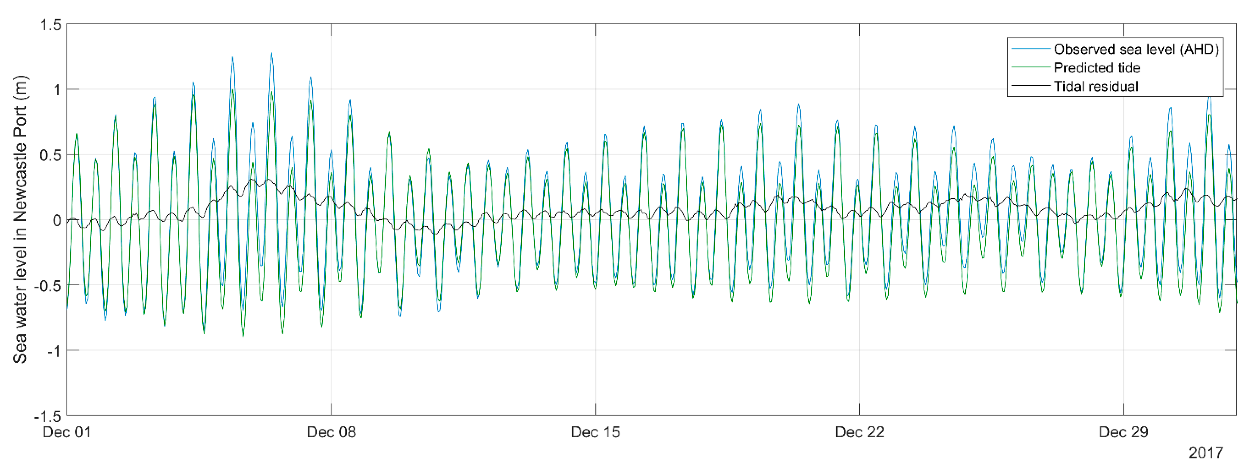
Figure A3.
Time-series of observed sea water levels in Newcastle Port during December 2017. The blue line indicates the observed water level. The green line indicates the predicted tide using Utide. The black line represents the obtained tidal residuals.
Figure A3.
Time-series of observed sea water levels in Newcastle Port during December 2017. The blue line indicates the observed water level. The green line indicates the predicted tide using Utide. The black line represents the obtained tidal residuals.

Figure A4.
Time-series of observed sea water levels in Patonga during December 2017. The blue line indicates the observed water level. The green line indicates the predicted tide using Utide. The black line represents the obtained tidal residuals.
Figure A4.
Time-series of observed sea water levels in Patonga during December 2017. The blue line indicates the observed water level. The green line indicates the predicted tide using Utide. The black line represents the obtained tidal residuals.

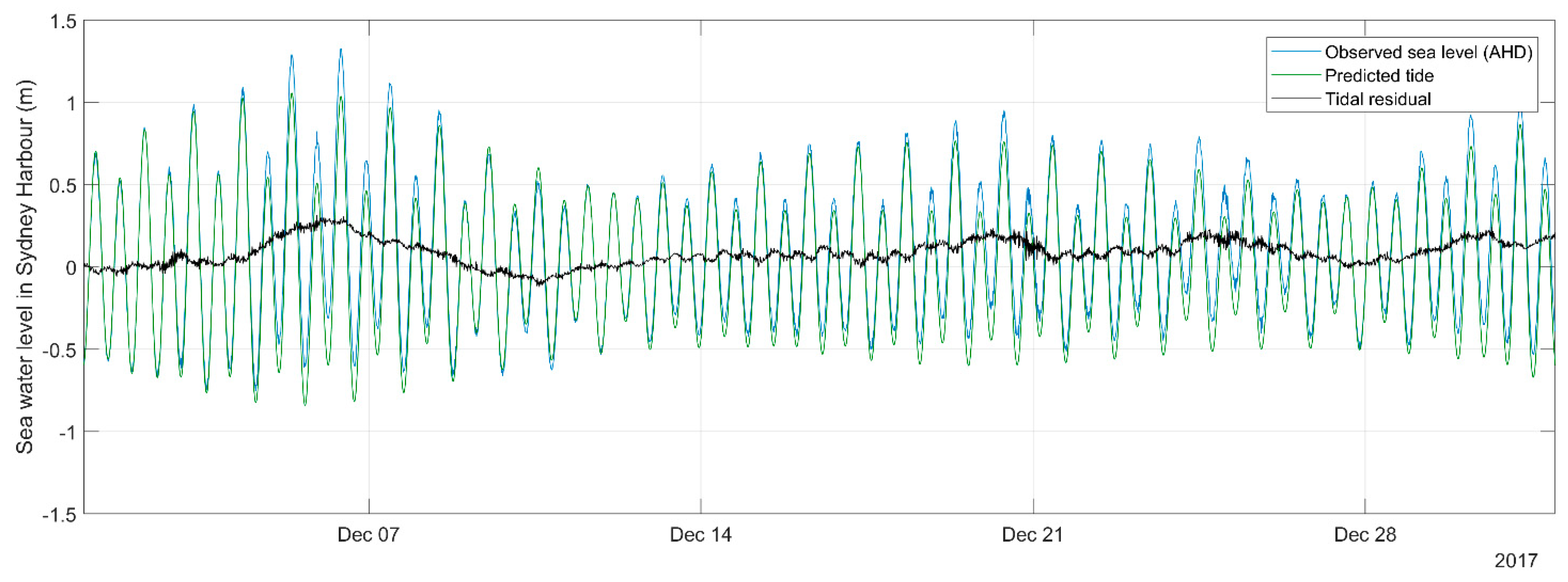
Figure A5.
Time-series of observed sea water levels in Sydney Harbour during December 2017. The blue line indicates the observed water level. The green line indicates the predicted tide using Utide. The black line represents the obtained tidal residuals.
Figure A5.
Time-series of observed sea water levels in Sydney Harbour during December 2017. The blue line indicates the observed water level. The green line indicates the predicted tide using Utide. The black line represents the obtained tidal residuals.

Figure A6.
Time-series of observed sea water levels in Fort Denison during December 2017. The blue line indicates the observed water level. The green line indicates the predicted tide using Utide. The black line represents the obtained tidal residuals.
Figure A6.
Time-series of observed sea water levels in Fort Denison during December 2017. The blue line indicates the observed water level. The green line indicates the predicted tide using Utide. The black line represents the obtained tidal residuals.

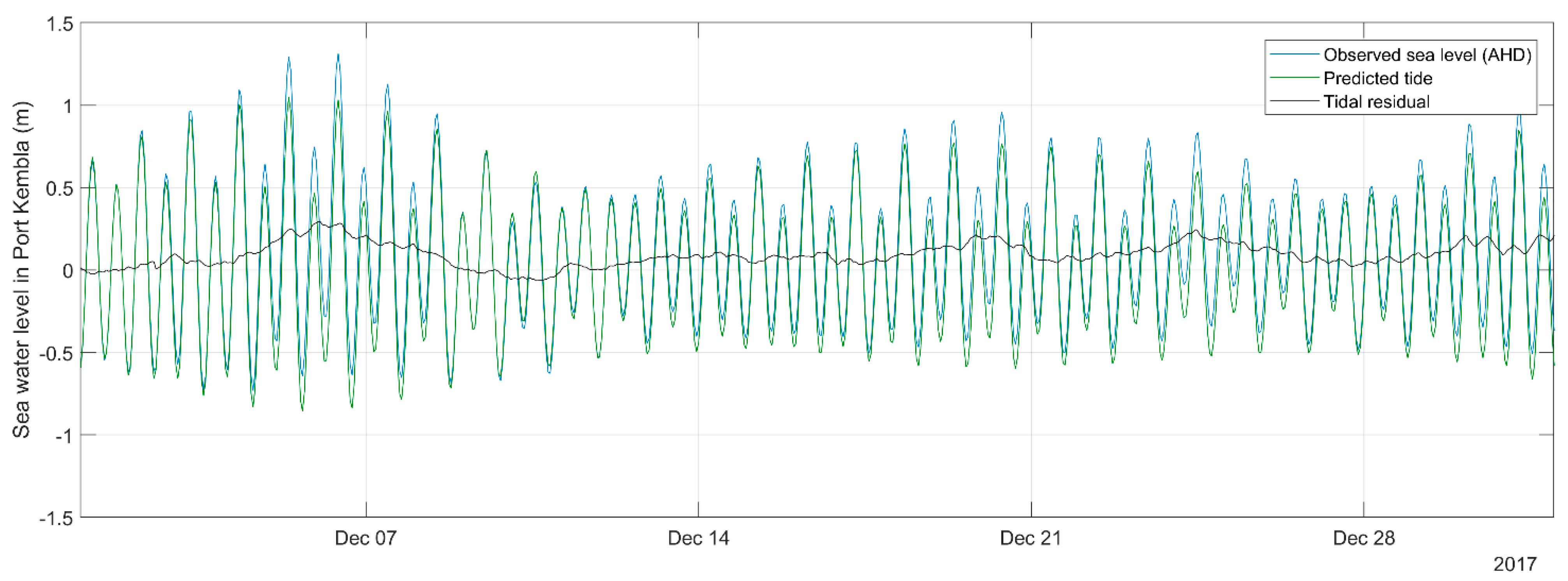
Figure A7.
Time-series of observed sea water levels in Port Kembla during December 2017. The blue line indicates the observed water level. The green line indicates the predicted tide using Utide. The black line represents the obtained tidal residuals.
Figure A7.
Time-series of observed sea water levels in Port Kembla during December 2017. The blue line indicates the observed water level. The green line indicates the predicted tide using Utide. The black line represents the obtained tidal residuals.

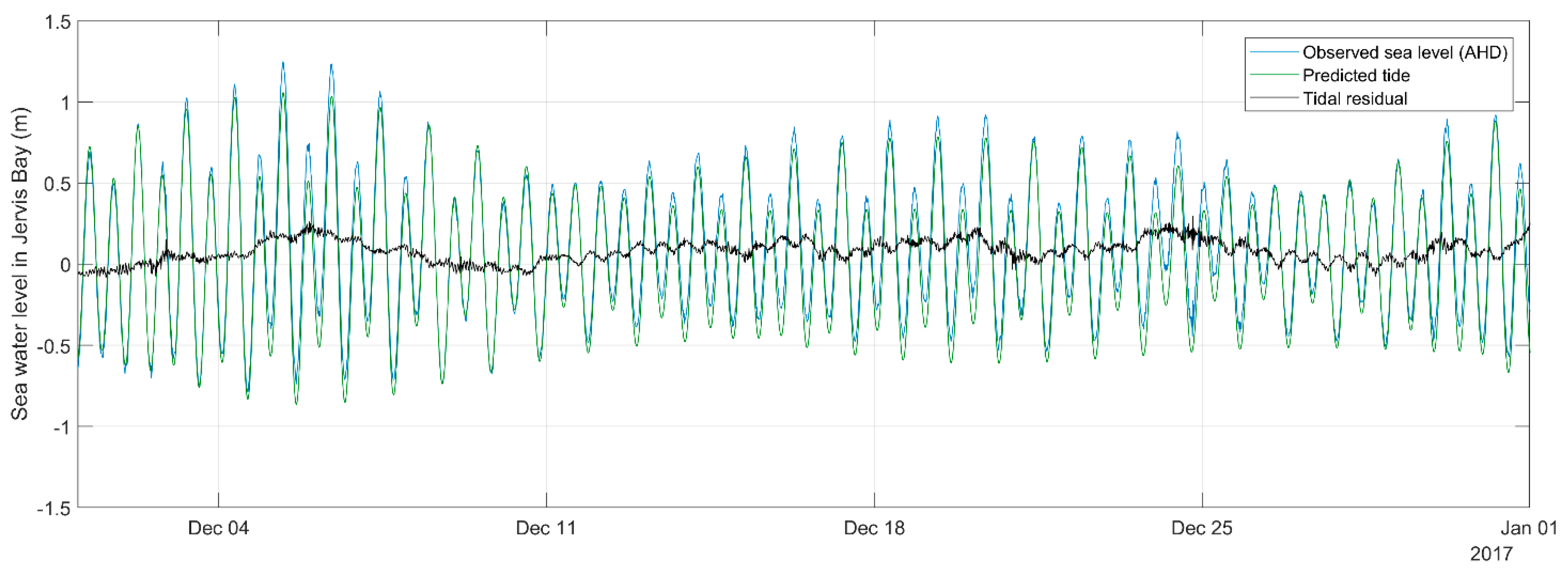
Figure A8.
Time-series of observed sea water levels in Jervis Bay during December 2017. The blue line indicates the observed water level. The green line indicates the predicted tide using Utide. The black line represents the obtained tidal residuals.
Figure A8.
Time-series of observed sea water levels in Jervis Bay during December 2017. The blue line indicates the observed water level. The green line indicates the predicted tide using Utide. The black line represents the obtained tidal residuals.

Figure A9.
Time-series of observed sea water levels in Eden during December 2017. The blue line indicates the observed water level. The green line indicates the predicted tide using Utide. The black line represents the obtained tidal residuals.
Figure A9.
Time-series of observed sea water levels in Eden during December 2017. The blue line indicates the observed water level. The green line indicates the predicted tide using Utide. The black line represents the obtained tidal residuals.

References
- Talke, S.A.; Jay, D.A. Nineteenth-century North American and pacific tidal data: Lost or just forgotten. J. Coast. Res. 2013, 29, 118–127. [Google Scholar] [CrossRef] [Green Version]
- Talke, S.A.; Jay, D.A. Changing Tides: The Role of Natural and Anthropogenic Factors. Ann. Rev. Mar. Sci. 2020, 12, 121–151. [Google Scholar] [CrossRef] [Green Version]
- Haigh, I.D.; Pickering, M.D.; Green, J.A.M.; Arbic, B.K.; Arns, A.; Dangendorf, S.; Hill, D.F.; Horsburgh, K.; Howard, T.; Idier, D.; et al. The Tides They Are A-Changin’: A Comprehensive Review of Past and Future Nonastronomical Changes in Tides, Their Driving Mechanisms, and Future Implications. Rev. Geophys. 2020, 58, 1–39. [Google Scholar] [CrossRef] [Green Version]
- Hanslow, D.J.; Morris, B.; Foulsham, E.; Kinsela, M.A. A Regional Scale Approach to Assessing Current and Potential Future Exposure to Tidal Inundation in Different Types of Estuaries. Sci. Rep. 2018, 8, 1–13. [Google Scholar] [CrossRef]
- Callaghan, D.P.; Couriel, E.; Hanslow, D.J.; Modra, B.; Fitzhenry, M.; Jacobs, R. Comparing extreme water levels using different techniques and impact of climate indices. In Proceedings of the Australasian Coasts and Ports 2017 Conference, Cairns, Australia, 21–23 June 2017; pp. 282–288. [Google Scholar]
- McPherson, B.; Young, S.; Modra, B.; Couriel, E.; You, B.; Hanslow, D.J.; Callaghan, D.P.; Baldock, T.; Nielsen, P. Penetration of Tides and Tidal Anomalies in New South Wales Estuaries. In Proceedings of the 2013 Australasian Coastal and Ocean Engineering Conference and the Australasian Port and Harbour Conference, Sydney, Australia, 11–13 September 2013; pp. 537–542. [Google Scholar]
- Pugh, D.T. Tides, Surges and Mean Sea-Level (Reprinted with Corrections); John Wiley and Sons: Chichester, UK, 1996. [Google Scholar]
- Egbert, G.D.; Ray, R.D. Tidal prediction. J. Mar. Res. 2017, 75, 189–237. [Google Scholar] [CrossRef]
- Foreman, M.G.G.; Henry, R.F. The harmonic analysis of tidal model time series. Adv. Water Resour. 1989, 12, 109–120. [Google Scholar] [CrossRef]
- MHL. Mid New South. Wales Coastal Region. Tide-Storm Surge Analysis; Manly Hydraulics Laboratory: Sydney, Australia, 1992.
- Horsburgh, K.; Wilson, C. Tide-surge interaction and its role in the distribution of surge residuals in the North Sea. J. Geophys. Res. Ocean. 2007, 112, 1–13. [Google Scholar] [CrossRef] [Green Version]
- Mawdsley, R.J.; Haigh, I.D. Spatial and temporal variability and long-term trends in skew surges globally. Front. Mar. Sci. 2016, 3, 1–17. [Google Scholar] [CrossRef] [Green Version]
- MHL. NSW Ocean. and River Entrance Tidal Levels Annual Summary 2016–2017; Manly Hydraulics Laboratory: Sydney, Australia, 2017.
- Modra, B.; Hesse, S. NSW Ocean Water Levels. In Proceedings of the 20th NSW Coastal Conference, Tweed Heads, Australia, 8–11 November 2011. [Google Scholar]
- MHL. Tide Gauge Histories Metadata for National and NDW Tide Gauges; Manly Hydraulics Laboratory: Sydney, Australia, 2013.
- Moftakhari, H.R.; Jay, D.A.; Talke, S.A.; Kukulka, T.; Bromirski, P.D. A novel approach to flow estimation in tidal rivers. Water Resour. Res. 2013, 49, 4817–4832. [Google Scholar] [CrossRef] [Green Version]
- Piecuch, C.G.; Bittermann, K.; Kemp, A.C.; Ponte, R.M.; Little, C.M.; Engelhart, S.E.; Lentz, S.J. River-discharge effects on United States Atlantic and Gulf coast sea-level changes. Proc. Natl. Acad. Sci. USA 2018, 115, 7729–7734. [Google Scholar] [CrossRef] [PubMed] [Green Version]
- Godin, G. The propagation of tides up rivers with special considerations on the upper Saint Lawrence river. Estuar. Coast. Shelf Sci. 1999, 48, 307–324. [Google Scholar] [CrossRef]
- Buschman, F.A.; Hoitink, A.J.F.; Van Der Vegt, M.; Hoekstra, P. Subtidal water level variation controlled by river flow and tides. Water Resour. Res. 2009, 45, 1–12. [Google Scholar] [CrossRef]
- Kukulka, T.; Jay, D.A. Impacts of Columbia River discharge on salmonid habitat: 2. Changes in shallow-water habitat. J. Geophys. Res. Ocean. 2003, 108, 1–16. [Google Scholar] [CrossRef] [Green Version]
- Cartwright, D.E.; Tayler, R.J. New Computations of the Tide-generating Potential. Geophys. J. R. Astron. Soc. 1971, 23, 45–73. [Google Scholar] [CrossRef] [Green Version]
- Foreman, M.G.G.; Cherniawsky, J.Y.; Ballantyne, V.A. Versatile harmonic tidal analysis: Improvements and applications. J. Atmos. Ocean. Technol. 2009, 26, 806–817. [Google Scholar] [CrossRef]
- Leffler, K.E.; Jay, D.A. Enhancing tidal harmonic analysis: Robust (hybrid L1/L2) solutions. Cont. Shelf Res. 2009, 29, 78–88. [Google Scholar] [CrossRef]
- Pawlowicz, R.; Beardsley, B.; Lentz, S.J. Classical tidal harmonic analysis including error estimates in MATLAB using T_TIDE. Comput. Geosci. 2002, 28, 929–937. [Google Scholar] [CrossRef]
- Codiga, D.L. Unified Tidal Analysis and Prediction Using the UTide Matlab Functions; University of Rhode Islan: Narragansett, RI, USA, 2011; p. 59. [Google Scholar]
- AHO. Australian National Tide Tables 2012; Australian Government, Department of Defence, Australian Hydrographic Service: Wollongong, Australia, 2011.
- Holbrook, N.J.; Goodwin, I.D.; McGregor, S.; Molina, E.; Power, S. ENSO to multi-decadal time scale changes in East Australian Current transports and Fort Denison sea level: Oceanic Rossby waves as the connecting mechanism. Deep Res. Part II Top. Stud. Oceanogr. 2010, 58, 547–558. [Google Scholar] [CrossRef]
- DCCEE. Climate Change Risks to Coastal Buildings and Infrastructure; Australian Government, Department of Climate Change and Energy: Canberra, Australia, 2011.
- McInnes, K.L.; White, C.J.; Haigh, I.D.; Hemer, M.A.; Hoeke, R.K.; Holbrook, N.J.; Kiem, A.S.; Oliver, E.C.J.; Ranasinghe, R.; Walsh, K.J.E.; et al. Natural hazards in Australia: Sea level and coastal extremes. Clim. Chang. 2016, 139, 69–83. [Google Scholar] [CrossRef] [Green Version]
- Couriel, E.; Modra, B.; Jacobs, R. NSW Sea Level Trends—The Ups and Downs. In Proceedings of the 17th Australian Hydrographers Association Conference, Sydney, Austrilia, 28–31 October 2014; pp. 1–19. [Google Scholar]
- MHL. NDRP Tailwater Project Stage 2; Manly Hydraulics Laboratory: Sydney, Australia, 2013.
- PSMSL. Permanent Service for Mean Sea Level. 2019. Available online: https://www.psmsl.org/ (accessed on 4 November 2019).
- Watson, P.J. Is there evidence yet of acceleration in mean sea level rise around Mainland Australia? J. Coast. Res. 2011, 27, 368–377. [Google Scholar] [CrossRef]
- Keysers, J.H.; Quadros, N.D.; Collier, P.A. Vertical Datum Transformations across the Littoral Zone Datum before Integrating Land Height Data with Near. 2012. Available online: www.crcsi.com.au (accessed on 20 May 2021).
- MHL. NSW Extreme Ocean. Water Levels; Manly Hydraulics Laboratory: Sydney, Australia, 2018.
- Mhl, R.; NSW Office. Review of NSW OEH Automatic Water Level Recorder Network; Manly Hydraulics Laboratory: Sydney, Australia, 2019.
- Matte, P.; Jay, D.A.; Zaron, E.D. Adaptation of Classical Tidal Harmonic Analysis to Nonstationary Tides, with Application to River Tides. J. Atmos. Ocean. Technol. 2013, 30, 569–589. [Google Scholar] [CrossRef] [Green Version]
- Matte, P.; Secretan, Y.; Morin, J. Temporal and spatial variability of tidal-fluvial dynamics in the St. Lawrence fluvial estuary: An application of nonstationary tidal harmonic analysis. J. Geophys. Res. Ocean. 2014, 3868–3882. [Google Scholar] [CrossRef] [Green Version]
- MHL. MHL Tidal Analysis Methodology Review; Manly Hydraulics Laboratory: Sydney, Australia, 2018.
- Bryant, E.A.; Kidd, R. Beach Erosion, May–June, 1974, Central and South Coast, NSW. 1975. Available online: https://ro.uow.edu.au/scipapers/64 (accessed on 20 May 2021).
- Woodham, R.; Brassington, G.B.; Robertson, R.; Alves, O. Propagation characteristics of coastally trapped waves on the Australian Continental Shelf. J. Geophys. Res. Ocean. 2013, 118, 4461–4473. [Google Scholar] [CrossRef]
- Speer, M.; Wiles, P.; Pepler, A. Low pressure systems off the New South Wales coast and associated hazardous weather: Establishment of a database. Aust. Meteorol. Oceanogr. J. 2009, 58, 29–39. [Google Scholar] [CrossRef]
- McInnes, K.L.; Hubbert, G.D. The impact of eastern Australian cut-off lows on coastal sea levels. Meteorol. Appl. 2001, 8, 229–243. [Google Scholar] [CrossRef]
- Mortlock, T.R.; Goodwin, I.D.; McAneney, J.K.; Roche, K. The June 2016 Australian East Coast Low: Importance of wave direction for coastal erosion assessment. Water 2017, 9, 121. [Google Scholar] [CrossRef]
- OEH. Eastern Seaboard Climate Change Initiative. East. Coast. Lows Research Program. Synthesis for NRM Stakeholders; Office of Environment and Heritage: Sydney, Australia, 2016.
- Hogarth, P.; Hughes, C.W.; Williams, S.D.P.; Wilson, C. Improved and extended tide gauge records for the British Isles leading to more consistent estimates of sea level rise and acceleration since 1958. Prog. Oceanogr. 2020, 184, 102333. [Google Scholar] [CrossRef]
- García, M.J.; Gómez, B.P.; Raicich, F.; Rickards, L.; Bradshaw, E.; Plag, H.P.; Zhang, X.; Bye, B.L.; Isaksen, E. European Sea Level monitoring: Implementation of ESEAS quality control. Int. Assoc. Geod. Symp. 2007, 130, 67–70. [Google Scholar]
- Pouliquen, S. Recommendations for In-Situ Data Real Time Quality Control. [Version 1.2]; EuroGOOS Publication Report No. 27. European Global Ocean Observing System (EuroGOOS), 2010. Available online: https://eurogoos.eu/download/recommendations-for-in-situ-data-real-time-quality-control/ (accessed on 13 September 2021).
Figure 1.
Spatial distribution, source, and type of NSW ocean tide gauge. (a) Satellite imagery of the coast of NSW with all existing ocean-tide gauges. The grey line represents the state boundary. (b) World map highlighting Australia and NSW. (c) Satellite imagery of the Tweed mouth region showing the OOO gauge. (d) Satellite imagery of the Greater Sydney area with the two OB gauges considered herein. Circles indicate OB gauges, the triangle indicates the ORE, and the hexagon indicates the OOO gauge. Green colour indicates gauges operated by MHL. Blue colour indicates gauges not operated by MHL.

Figure 2.
Years of operation and data availability for each ocean tide gauge assessed herein. The thick black line indicates the period of recorded data. Discontinuities in the thick black line indicate periods of missing data. Gauges are shown from north (top) to south (bottom). Note that data for Fort Denison before 1914 (not used) are not shown owing to their unreliability.

Figure 3.
Hydrographic map of the Hunter and the Tweed regions, with the locations of the auxiliary gauges, the source, and category for flood control. (a) NSW state is shown in white, while other states are in grey; the red area represents the two river catchments. (b) The blue line represents the Tweed River streams; the grey contour is the catchment boundary for the primary control gauge. (c) The blue line represents the Hunter River streams; the grey contour is the catchment boundary for the primary control gauge. For a global reference, see Figure 1.

Figure 4.
Water level records at two water level (auxiliary) gauges on Hunter River (turquoise lines). (a) Water level data at Greta. Mean plus 2 standard deviations (black dashed line); 2.5 standard deviations (solid black line); and 3 standard deviations (black dashed-dotted line). (b) The water level at Raymond Terrace. Mean plus 2 standard deviations (black dashed line); 2.5 standard deviations (black solid line); and 3 standard deviations (black dashed-dotted line).

Figure 5.
Water level records at two water level gauges on the Tweed River (turquoise lines). (a) Water level data at Tumbulgum. Mean plus 2 standard deviations (black dashed line); 2.5 standard deviations (solid black line); and 3 standard deviations (black dashed-dotted line). (b) Water level at Murwillumbah. Mean plus 2 standard deviations (black dashed line); 2.5 standard deviations (solid black line); and 3 standard deviations (black dashed-dotted line).

Figure 6.
(a) Satellite imagery of the Tweed River mouth, showing the locations of gauges used for the adjustment of the offshore dataset. (b) Regression line (solid black line), with the data density increasing from blue to red. (c) A section of the 15-min water level record at the two onshore river entrance gauges on Tweed River: Tweed Entrance South (turquoise line) and Tweed Heads (black dashed line); and the correlation of the two gauges between 2014 and 2015.

Figure 7.
Statistical correlation between the mean water level for each offshore gauge deployment period at Letitia 2A and Tweed Entrance. The turquoise line indicates the regression line (R2 = 0.4315, y = 0.56x − 0.01523, p-value = 0.0001). The black points indicate the distribution of the mean water levels during each deployment.

Figure 8.
Mean sea levels during deployment at gauges on the Tweed River mouth area. (a) Original Tweed Entrance (solid black line), Letitia 2A (solid blue line), and the periods of missing data are shown in the grey boxes. (b) Filled Tweed Entrance (dashed black line), Tweed Heads Offshore (turquoise line), and original Tweed Entrance South (solid black line).

Figure 9.
Comparison between yearly averaged tidal residuals at four locations showing tidal residuals averaged from tidal residual records provided by Manly Hydraulics Laboratory (turquoise line) and tidal residuals averaged from tidal residuals obtained in Utide without accounting for the sea level rise (solid black line) and accounting for the sea level rise (dashed black line). Gauges are shown from north (top) to south (bottom).

Figure 10.
Verification of the Utide model. Comparisons between the obtained tidal residuals and tidal residuals provided by MHL at four locations. (Left) regression line (turquoise); distribution of records for 90–95% of the available data (light blue), for 95–99% of the available data (navy blue), and 99–100% of the available data (black). (Right) histogram of differences between yearly averaged tidal residuals obtained from tidal residuals provided by Manly Hydraulics Laboratory and obtained from Utide. Data are binned in intervals of 0.0005 m. Gauges are shown from north (top) to south (bottom).

Figure 11.
Obtained tidal residuals for the seven ocean tide gauge datasets with approximately 30-year record lengths. (Left): histograms of the frequency distribution of the tidal residuals. Data are binned in intervals of 0.01 m. (Right): time-series of the tidal residuals. Gauges are shown from north (top) to south (bottom).

Figure 12.
Obtained tidal residual for the datasets with at least 50 years of record length. (Left) histograms of the frequency distribution of the tidal residuals. Data are binned in intervals of 0.01 m. (Right) time-series of the tidal residuals. Gauges are shown from north (top) to south (bottom).

Figure 13.
Distribution of water levels and tidal residuals. (a) Distribution of water levels: dark blue indicates negative values, and purple indicates positive values. (b) For each water level, positive and negative tidal residuals were obtained: for negative water levels, light blue indicates negative tidal residuals and blue indicates positive tidal residuals; for positive water levels, magenta indicates negative tidal residuals, and pink indicates positive tidal residuals. (c) Distribution of tidal residuals: navy blue indicates negative values, and light purple indicates positive values.

Figure 14.
Histogram of monthly minimum (green), mean (blue), and maximum values (purple) for datasets with approximately 30-year records. Histogram of the frequency distribution of tidal residuals (top). Histogram of the frequency distribution of total water levels (bottom). Data are binned in intervals of 0.03 m. Gauges are shown from south (left) to north (right).

Figure 15.
Histogram of monthly minimum values (green), mean values (blue), and maximum values (purple) for datasets with at least 50-year records. Histogram of the frequency distribution of tidal residuals (top). Histogram of the frequency distribution of total water levels (bottom). Data are binned in intervals of 0.03 m. Gauges are shown from south (left) to north (right).

Figure 16.
Maximum, mean, and minimum monthly values for NSW ocean tide gauges with at least 50-year records. The blue line indicates maximum values, the black line indicates mean values, and the turquoise line indicates minimum values. Solid lines indicate tidal residuals and dashed lines indicate total/observed water levels.

Figure 17.
Monthly tidal residuals for NSW ocean tide gauges during two distinct El Niño Southern Oscillation (ENSO) phases: coloured boxes delineate the ENSO events according to the Bureau of Meteorology. The 1997–1998 El Niño (left red box) and 2010–2012 La Niña (right blue box) phases are shown. The blue line indicates maximum values, the black line indicates mean values, and the turquoise line indicates minimum values. (a) the five northern gauges are shown from north (top) to south (bottom). (b) the four southern gauges are shown from north (top) to south (bottom).


Figure 18.
Elevated water levels and tidal residuals on the NSW coast during the May 2015 continental shelf wave (CSW). The blue line indicates the observed water levels, and the black line indicates the obtained tidal residuals. Gauges are shown from north (top) to south (bottom).
Figure 18.
Elevated water levels and tidal residuals on the NSW coast during the May 2015 continental shelf wave (CSW). The blue line indicates the observed water levels, and the black line indicates the obtained tidal residuals. Gauges are shown from north (top) to south (bottom).

Figure 19.
Elevated water levels and tidal residuals on the NSW coast during the April 2015 east coast low (ECL) in the central coast. (a,b) The blue line indicates observed water levels and the black line indicates obtained tidal residuals. Gauges are shown from north (top) to south (bottom). (c) Synoptic chart of 21 April 2015, the day of the water level peak (Source: BoM).

Table 1.
List of the datasets presented in this study in alphabetic order. The source, sampling frequency, length of the record, record gaps, and gauge type are indicated. Gauge types are as follows: onshore bay or harbour (OB), onshore river entrance (ORE), and offshore open ocean (OOO).
Table 1.
List of the datasets presented in this study in alphabetic order. The source, sampling frequency, length of the record, record gaps, and gauge type are indicated. Gauge types are as follows: onshore bay or harbour (OB), onshore river entrance (ORE), and offshore open ocean (OOO).
| Name | Source | Sampling Frequency (Minutes) | Record Length (Years) | Available Data (%) | Type |
|---|---|---|---|---|---|
| Crowdy Head | MHL | 15 | 34 | 88.73 | OB |
| Eden | MHL | 15 | 34 | 92.82 | OB |
| Fort Denison | BoM | 60 | 106 | 98.16 | OB |
| Jervis Bay | MHL | 15 | 31 | 90.76 | OB |
| Newcastle Port | BoM | 60 | 63 | 83.24 | ORE |
| Patonga | MHL | 15 | 28 | 98.00 | OB |
| Port Kembla | BoM | 60 | 63 | 65.81 | OB |
| Sydney Harbour | MHL | 15 | 33 | 96.06 | OB |
| Tweed Heads Offshore | MHL | 60 | 33 | 96.12 | OOO |
Table 2.
Auxiliary gauges used for flood removal in the ORE gauge and datum adjustment of the OOO gauge datasets, listed in alphabetic order. The source, sampling frequency, length of the record, record gaps, and gauge type are indicated. The sampling frequency is indicated in minutes, the record length is given in years, and the availability of the data is given as a percentage of the entire record. The gauge types are as follows: onshore river entrance (ORE) and water level.
| Name | Source | Sampling Frequency (Minutes) | Record Length (Years) | Available Data (%) | Type |
|---|---|---|---|---|---|
| Greta | BoM | 60 | 48 | 99.73 | Water level |
| Letitia 2A | MHL | 15 | 30 | 88.30 | Water level |
| Murwillumbah | MHL | 15 | 25 | 90.95 | Water level |
| Raymond Terrace | MHL | 15 | 32 | 97.94 | Water level |
| Tumbulgum | MHL | 15 | 32 | 90.19 | Water level |
| Tweed Heads | MHL | 15 | 24 | 78.18 | Water level |
| Tweed Entrance South | MHL | 15 | 3 | 99.79 | ORE |
Publisher’s Note: MDPI stays neutral with regard to jurisdictional claims in published maps and institutional affiliations. |
© 2021 by the authors. Licensee MDPI, Basel, Switzerland. This article is an open access article distributed under the terms and conditions of the Creative Commons Attribution (CC BY) license (https://creativecommons.org/licenses/by/4.0/).
Share and Cite
MDPI and ACS Style
Viola, C.N.A.; Verdon-Kidd, D.C.; Hanslow, D.J.; Maddox, S.; Power, H.E. Long-Term Dataset of Tidal Residuals in New South Wales, Australia. Data 2021, 6, 101. https://0-doi-org.brum.beds.ac.uk/10.3390/data6100101
AMA Style
Viola CNA, Verdon-Kidd DC, Hanslow DJ, Maddox S, Power HE. Long-Term Dataset of Tidal Residuals in New South Wales, Australia. Data. 2021; 6(10):101. https://0-doi-org.brum.beds.ac.uk/10.3390/data6100101
Chicago/Turabian StyleViola, Cristina N. A., Danielle C. Verdon-Kidd, David J. Hanslow, Sam Maddox, and Hannah E. Power. 2021. "Long-Term Dataset of Tidal Residuals in New South Wales, Australia" Data 6, no. 10: 101. https://0-doi-org.brum.beds.ac.uk/10.3390/data6100101