The Effect of Preprocessing Techniques, Applied to Numeric Features, on Classification Algorithms’ Performance

Abstract

It is recognized that the performance of any prediction model is a function of several factors. One of the most significant factors is the adopted preprocessing techniques. In other words, preprocessing is an essential process to generate an effective and efficient classification model. This paper investigates the impact of the most widely used preprocessing techniques, with respect to numerical features, on the performance of classification algorithms. The effect of combining various normalization techniques and handling missing values strategies is assessed on eighteen benchmark datasets using two well-known classification algorithms and adopting different performance evaluation metrics and statistical significance tests. According to the reported experimental results, the impact of the adopted preprocessing techniques varies from one classification algorithm to another. In addition, a statistically significant difference between the considered data preprocessing techniques is demonstrated.

1. Introduction

Data are not always “clean”; the presence of redundant, inconsistent, noisy, and/or missing data in a dataset indicates that data are not clean and need to be handled before applying any machine learning algorithm. Data preprocessing is concerned with solving such issues. In addition, data normalization, discretization, and transformation are data preprocessing tasks. Thus, data preprocessing is a significant step for Knowledge Discovery in Database (KDD). More specifically, the performance of machine learning algorithms is strongly influenced by the adopted preprocessing techniques [1]. Some researchers argue that adopting particular data preprocessing technique relies primarily on the considered dataset [2], while others claim that the selection should be based on experiments [3].

With respect to numerical features, data normalization and handling missing values are considered the main preprocessing issues especially when the adopted classification algorithm was originally designed to handle numerical features. The reason behind the importance of the normalization process with respect to the performance of classification algorithms is that features assigned “small-range” values are dominated by features with “large-range” values; consequently, the small-range features have no influence on the classification process [4,5]. Results from previous research showed that feature normalization has a significant impact on classification accuracy [2,3,4,6,7,8]. Regarding missing values, the“bad” treatment of missing data results in a degradation in classification accuracy, especially when the considered dataset contains a high missing values rate [9,10,11]. Therefore, handling missing values carefully during preprocessing is considered a necessary step in order to obtain a high performance classification model. Much research work has studied the effect of various normalization techniques or handling missing values strategies on classification performance separately; however, few works have evaluated the impact of combining normalization and handling missing values techniques. In addition, less attention has been given to the effect of different treatments of missing values or normalization techniques on classification efficiency.

The main motivation for the work presented in this paper is the desire to supply machine learning researchers and users with recommendations regarding the preprocessing techniques to be adopted in order to obtain high performance classification models. Thus, this paper investigates the impact of combining several preprocessing techniques, related to normalization and dealing with missing values, on the performance of classification algorithms.

In this research, three well-known normalization techniques: (i) min-max normalization, (ii) Z-score normalization, and (iii) decimal scaling normalization are evaluated. With respect to handling missing values, for numeric dimensions, three well-known strategies are evaluated: (i) discarding instances that include missing values, (ii) replacing missing values with the feature mean, and (iii) using the k-Nearest Neighbor (kNN) algorithm to replace missing values. Two alternative classification algorithms are considered to generate the prediction models after applying the preprocessing techniques: (i) Support Vector Machines (SVMs) and (ii) Artificial Neural Networks (ANNs). As a result, nine variations of preprocessing combinations are evaluated for each classification algorithm. It is worth noting here that some classification algorithms were originally designed to handle numerical data, for example kNN and SVM. However, such algorithms can be adapted to handle categorical data. Other classification algorithms were originally designed to handle categorical data; examples include decision tree, naive Bayes, and rule based classifiers. However, such algorithms can be adapted to handle numerical data. In the research presented in this paper, classification algorithms that were originally designed to handle numerical data are considered. It is expected that these algorithms will be affected by the normalization process due to: (i) being originally designed to handle numerical features (the nature of the algorithm) and (ii) applying some calculations on numerical features, like distance computation.

In order to determine if one technique significantly outperforms another (others), the Friedman statistical test [12] and the Nemenyi post-hoc test [13] have been applied. From the foregoing, the objectives of the work presented in this paper can be summed up as follows:

• We evaluate the effect of combining several preprocessing techniques, applied to numerical features, on the performance of classification algorithms.
• We find the optimal combination of preprocessing techniques, with respect to the numerical values, that results in more accurate classification.

The above-mentioned objectives can be articulated by the following big question:

“What are the most convenient techniques that can be adopted to produce high performance classification models in terms of classification effectiveness and efficiency?”

The remainder of this paper is organized as follows: Section 2 provides the required background to the work described in this paper and discusses the previous work that studied the effect of preprocessing techniques on the performance of classification models. Section 3 describes the datasets that have been used to evaluate the considered preprocessing techniques. Section 4 presents the adopted experimental methodology. Section 5 presents and discusses the obtained results. Finally, Section 6 concludes the discussion and provides directions for further work.

2. Related Work

This section provides a review of preprocessing techniques, normalization, and handling missing values with respect to numerical attributes. In addition, the section presents a summary of related work on the effect of preprocessing techniques on the performance of classification algorithms. The section is organized as follows: Section 2.1 provides an overview of data normalization techniques, while Section 2.2 presents an overview of the missing values problem and the most common ways to deal with it. A summary of the previous related work on the effect of preprocessing techniques on the performance of classification algorithms is presented in Section 2.3.

2.1. Normalization

Data normalization is a preprocessing technique applied to numerical features before applying classification or clustering algorithms that are mainly designed to handle numerical features. The reason behind the importance of the normalization process is to avoid a number of the considered features concealing the effect of others, particularly when features have different varying ranges. On the other hand, selecting the normalization technique and normalization range (interval) is considered a significant step during the preprocessing stage, due to the “change” that affects the considered data and consequently the results of the machine learning algorithm that will be applied after preprocessing [3]. The most widely used data normalization techniques are [5]:

• Min-max normalization: This is one of the most common techniques to normalize data, in which values for the considered feature are transformed to new smaller ones within a predefined interval, usually [0–1] is adopted [5]. It is recognized that min-max normalization maintains all the relationships in the considered data [6]. Each value in the considered feature is mapped to a new normalized value according to the following equation [5]:

  $$v^{\prime }=\frac{v-mi{n}_A}{ma{x}_A-mi{n}_A}(new\_ma{x}_A-new\_mi{n}_A)+new\_mi{n}_A$$

  (1)

  where $v^{\prime }$ is the new normalized value, v is the original value for the given feature, $ma{x}_A$ is the maximum value for the given feature A, $mi{n}_A$ is the minimum value for the given feature A, while $new\_ma{x}_A$ and $new\_mi{n}_A$ represent the maximum and minimum values for the new considered range.
• Z-score normalization: This is a statistical normalization technique that handles the outlier issue [5]. The mean and standard deviation for the considered feature are used to transform the feature values. More specifically, values for the considered feature are transformed into new normalized values by applying the following equation [5]:

  $$v^{\prime }=\frac{v-\mu }{\sigma }$$

  (2)

  where $\mu$ is the mean value of the designated feature and $\sigma$ is the standard deviation of the considered feature. Applying the Z-score normalization technique, values below the mean appear as negative numbers, values above the mean as positive numbers, while values that are exactly equal to the mean are mapped to zero.
• Decimal normalization: This is a normalization technique that normalizes the designated feature by moving the decimal point of the feature values, where the maximum absolute value of the considered feature determines the decimal point movement. Each value in the designated feature is mapped to a new normalized value according to the following equation [5]:

  $$v^{\prime }=\frac{v}{{10}^j}$$

  (3)

  where j is the smallest integer to get max ($|v^{\prime }|$) < 1.

2.2. Handling Missing Values

Missing data are recognized as one of the significant issues that should be handled carefully during the preprocessing stage, before applying machine learning algorithms, to obtain effective machine learning models. In practice, a dataset may contain missing data that are generated due to several reasons such as human errors, equipment faults, data unavailability (some people reject providing a value for specific features), and data not being up-to-date or inconsistent with other existing data (consequently removed). In addition, the detection of a data anomaly can be considered a reason for missing values, where the anomalous values are deleted and replaced with new values using a repairing mechanism [14]. The rates of missing values can be categorized as follows [15]:

• “Trivial”, where 1% of the data are missing.
• “Manageable”, where 1–5% of the data are missing.
• “Sophisticated”, where 5–15% of the data are missing; therefore sophisticated methods are required to handle this.
• “Severe”, more than 15% of the data are missing; thus, the serious influence of any applied technique would be noted.

In this paper, all rates were used in the experiments and taken into consideration.

According to the literature, the most widely used strategies to deal with missing values are [5,15,16,17]:

• Deleting an instance: Instances with missing values for at least one feature are deleted (ignored); this technique is the default option to deal with missing values with respect to many statistical packages [18,19].
• Filling manually: The missing values are filled manually; therefore, it is considered not efficient and not feasible especially when handling datasets that include a high missing values rate.
• Replacing with a global constant: A global value is utilized to fill in the missing values such as “unknown”.
• Replacing with the mean: The mean for a specific feature is used to fill in any missing values for that feature; this technique is also referred to as “maximum likelihood” [20]. Several variations of this technique are available. One variation utilizes the feature mean for all instances belonging to the same class label instead of the mean of all instances to fill in missing values.
• Using a prediction model: The decision tree, regression, and Bayesian models can be adopted to predict the missing values. Recent studies have used deep neural networks to repair data because neural networks can handle natural data that include missing values perfectly [21].
• Adopting an imputation procedure: The missing values are estimated based on a specific procedure, the most widely used procedure being k-Nearest Neighbor (kNN). Adopting the kNN procedure, missing values are imputed according to the most similar instances, where the distance measure (such as the Euclidean or Manhattan distance) is used to determine the most similar instances. Moreover, the repairing mechanisms adopted for handling anomalous data can be considered as one of the imputation procedures that exploit observations of the same data features in nearby locations [14]. Note here that Points 4, and 5 can be considered as imputation processes and coupled with this point.
• Adopting multiple imputation procedure: Multiple simulated variations of the considered dataset are produced and analyzed; after that, the results are joined together in order to output the inference [16].

Among the previous strategies, discarding an instance, replacing with the mean, and kNN imputation are considered the most common strategies for dealing with missing values and also available in most data mining tools. Thus, those techniques are considered in the work presented in this paper.

2.3. Previous Work on the Impact of Preprocessing Techniques on the Performance of Classification Algorithms

This section discusses the previous work that studied the effect of preprocessing techniques on the performance of classification models. Many techniques have been proposed to normalize data and deal with missing values. Several experimental studies tried to find the “best” technique to be used before applying classification algorithms; thus, a better prediction can be obtained. According to the literature, the research on the effect of preprocessing techniques on the performance of classification algorithms can be summarized as follows:

• Each research work evaluated various data preprocessing techniques. More specifically, some studies evaluated a number of normalization techniques, and some others evaluated some ways for dealing with missing data. Note here that only one reference was found by the author that evaluated the effect of normalization and handling missing values on classification accuracy using only one medical dataset [6]. In this research work, we focus on the most widely used preprocessing techniques with respect to numerical variables.
• Most research works were focused primarily on a specific classification algorithm. More specifically, with respect to normalization, most experiments were conducted to evaluate the impact on the performance of Support Vector Machine (SVM) or Artificial Neural Networks (ANNs) such as the work presented in [3,6,22,23]. On the other hand, with respect to handling missing values, experiments were conducted using rule-based, Decision Tree (DT), or kNN classifiers such as the work presented in [15,16,24].
• With respect to normalization, the evaluation in most research works was conducted using a specific dataset such as a hyperspectral dataset [4,22], a medical dataset [3,6,7,25], or a direct marketing dataset [2]. Only a few researchers have studied the effect of normalization on classification performance using several general datasets such as the experimental study presented in [23]. On the other hand, related work on handling missing values can be categorized into three categories according to the utilized datasets: (i) research work that utilized datasets with missing values in their original form [26,27], (ii) research work that utilized datasets with no missing values in their original form (missing values are generated artificially) [28], and (iii) research work that utilized datasets with and without missing values in their original form [15].
• With respect to handling missing values, as noted earlier, instrument failure is considered one of the main reasons for finding missing values in the datasets. Sensors are one of the instruments that are subject to failure for several reasons including environmental factors. Recently, several researchers have directed their research work toward handling missing or corrupted data resulting from sensor failures [29,30]. The field of renewable energy forecasting [31,32] is considered an example of this case, where the data are collected by geographically distributed sensors [33]. In order to handle the missing values in such datasets, some researchers replaced them with the mean of the same attribute observed for the same month of the same year at the same hour [33]. Moreover, linear interpolation, mode imputation, k-nearest neighbors, and multivariate imputation by chain equations (MICEs) are also used to solve the missing values problem with respect to renewable energy forecasting [29].
• Most research works used evaluation measures that evaluate the accuracy of the classifiers (such as the error rate and accuracy), while efficiency measures were not taken into consideration (such as model generation time or prediction time).
• Most research works did not consider statistical tests to rigorously compare the performance of different preprocessing techniques.

In the context of the work described in this paper, several combinations of normalization techniques and handling missing values strategies are investigated using two well-known classification algorithms and eighteen benchmark datasets from different disciplines and feature various characteristics. Additionally, different evaluation measures and statistical tests are adopted during the evaluation process.

3. Evaluation Datasets

This section provides a description of the main characteristics of the evaluation datasets. Eighteen datasets from different disciplines with various numbers of instances, class labels, and features were taken from the University of California Irvine (UCI) machine learning repository [34].

Table 1. The evaluation datasets’ description.

Dataset	Instance #	Classes #	Feature #	Features Type (Numerical, Nominal)	Missing Values (in All, in Numerical)	Missing Values Rate (%)	Area
Automobile	205	4	25	(15, 10)	(59, 57)	1.5	Life
ChronicKidneyDisease	400	2	24	(11, 14)	(1012, 778)	9.5	Medicine
Credit Approval	690	2	15	(6, 9)	(67, 25)	0.65	Financial
Cylinder Bands	540	2	35	(22, 13)	(999, 571)	5.30	Physical
Dermatology	366	6	34	(1, 33)	(8, 8)	0.06	Medicine
HCC survival	165	2	49	(26, 23)	(826, 475)	10.22	Medicine
Hepatitis	155	2	19	(6, 13)	(167, 122)	5.67	Medicine
MammographicMasses	961	2	5	(1, 4)	(162, 83)	3.37	Medicine
Thyroid (sick)	3772	2	29	(7, 22)	(6064, 5914)	2.17	Medicine
Abalone	4178	28	8	(7, 1)	None	0	Wildlife
Ecoli	336	8	7	(7,0)	None	0	Biology
PenDigits	10,992	10	16	(16,0)	None	0	Computer
Glass	214	6	9	(9, 0)	None	0	Physical
Page Blocks	5473	5	10	(10, 0)	None	0	Computer
Waveform	5000	3	21	(21, 0)	None	0	Physical
Vehicle	846	4	18	(18,0)	None	0	Computer
Online Shoppers’	12,330	2	17	(10, 7)	None	0	Business
Purchasing Intention

presents the main characteristics of the evaluation datasets. Recall that the research presented in this paper is concerned with the effect of different preprocessing techniques on classification performance with respect to numerical features; the considered datasets include at least one numerical feature. In addition, to precisely study the effect of diverse treatments of missing values on classification performance, nine of the considered datasets contain missing values (“original missing values”), while the remaining nine do not. The objective behind choosing datasets with “no missing” values is to artificially generate various rates of missing values; thus, a deeper and more comprehensive investigation can be achieved.

4. The Adopted Experimental Methodology

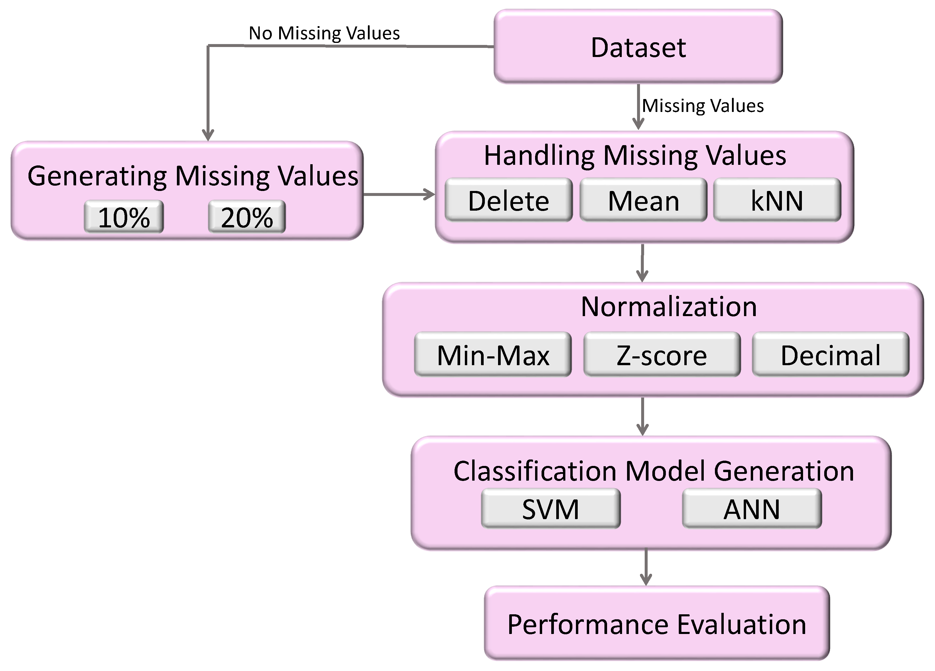
This section presents the adopted experimental methodology. Figure 1 summarizes the entire methodology. As shown in Figure 1, and as recognized, the generation of classification models commences with acquiring a dataset. Recall that eighteen benchmark datasets from various disciplines are considered. As noted in the previous section, the evaluation datasets can be categorized into two categories according to the inclusion of missing values: original missing values and no missing values. The first step in the adopted preprocessing strategy is to artificially introduce missing values for datasets that do not feature missing values. Two different rates are adopted to generate missing values: 10% sophisticated and 20% severe rates, respectively (see the literature review).

Now, the dataset includes missing values and is ready to be treated using one of the missing values treatment strategies (deleting instances that include missing values, replacing missing values with the feature mean, and using the k-Nearest Neighbor (kNN) algorithm). The next step is the normalization process, where the given dataset is normalized using one of the normalization techniques (min-max, Z-score and decimal). Consequently, nine alternative data preprocessing combination techniques are applied for each dataset: (i) Delete&MinMaxcombination technique, (ii) Delete&Z-score combination technique, (iii) Delete&Decimal combination technique, (iv) Mean&MinMax combination technique, (v) Mean&Z-score combination technique, (vi) Mean&Decimal combination technique, (vii) kNN&MinMax combination technique, (viii) kNN&Z-score combination technique, and (ix) kNN&Decimal combination technique.

After that, the considered classification algorithms (SVM and ANN) are applied to each dataset variation in order to generate the desired classification model. The final step in the adopted methodology is the evaluation process in which the performances of the resulting classification models are compared. Concerning effectiveness evaluation, accuracy and Area Under the receiver operating Curve (AUC) [35] measures are considered. On the other hand, model construction time is adopted to evaluate the efficiency. In addition, a statistical significance test is applied to the obtained results to ensure a more precise comparison.

5. Experiments and Evaluation

The well-known Weka data mining tool [36] was used for data preprocessing and classification models’ generation. All experiments were executed utilizing Intel(R) Core(TM) i7-4600U [email protected] 2.70 GHz with 8 GB RAM memory, running Windows 7 Professional. Ten-fold Cross-Validation (TCV) was adopted to obtain accurate results. Despite including average accuracy and average AUC results, the analysis was based on the average AUC because the AUC is a more precise measure than accuracy for comparing machine learning algorithms [35,37].

As noted earlier, in total, nine data preprocessing combination techniques are considered for each dataset with respect to each classification algorithm. In the context of the dataset with “no missing” values, the nine different data preprocessing combination techniques are applied to: (i) datasets having 10% missing values generated artificially and (ii) datasets having 20% missing values generated artificially.

Thus, the obtained results are organized in the following sub-sections as follows: Section 5.1 presents the obtained results using datasets that originally included missing values with respect to the nine alternative data preprocessing combination techniques and the two classification algorithms (ANN and SVM). Section 5.2 presents the obtained results using datasets that include 10% missing values that were generated artificially with respect to the nine alternative data preprocessing combination techniques and the two classification algorithms (ANN and SVM). Section 5.3 presents the obtained results using datasets that that include 20% missing values (generated artificially) with respect to the nine alternative data preprocessing combination techniques and the two classification algorithms (ANN and SVM). Section 5.4 discusses the classification models’ efficiency based on model generation time.

5.1. Results Obtained from Datasets Having Missing Values Originally

We commence with the results obtained when using the ANN classification algorithm coupled with the nine alternative data preprocessing combination techniques.

Table A1. Average accuracy and AUC values obtained using the ANN classification algorithm coupled with the nine data preprocessing techniques with respect to the datasets that featured missing values originally.

	ANN Classification
Technique	$\mathit{Delete}\&$		$\mathit{Delete}\&$		$\mathit{Delete}\&$		$\mathit{Mean}\&$		$\mathit{Mean}\&$		$\mathit{Mean}\&$		$\mathit{kNN}\&$		$\mathit{kNN}\&$		$\mathit{kNN}\&$
	$\mathit{MinMax}$		$\mathit{Zscore}$		$\mathit{Decimal}$		$\mathit{MinMax}$		$\mathit{Zscore}$		$\mathit{Decimal}$		$\mathit{MinMax}$		$\mathit{Zscore}$		$\mathit{Decimal}$
Dataset	Acc.	AUC	Acc.	AUC	Acc.	AUC	Acc.	AUC	Acc.	AUC	Acc.	AUC	Acc.	AUC	Acc.	AUC	Acc.	AUC
Automobile	82.39	0.929	86.16	0.947	69.81	0.880	79.51	0.923	79.02	0.929	73.17	0.881	79.02	0.920	78.54	0.920	73.17	0.880
Kidney	99.37	1.000	100.00	1.000	99.36	1.000	98.25	0.999	97.50	0.999	97.50	0.991	98.75	1.000	98.50	0.999	97.00	0.985
Credit	85.15	0.902	83.46	0.908	85.60	0.901	83.33	0.903	83.04	0.902	83.91	0.899	83.91	0.904	82.61	0.899	83.33	0.901
Cylinder	72.20	0.726	73.29	0.762	72.56	0.740	75.37	0.823	75.93	0.831	71.30	0.769	75.74	0.814	77.04	0.841	75.56	0.803
Dermatology	97.49	0.997	97.49	0.997	96.93	0.997	97.27	0.997	97.54	0.997	97.54	0.998	97.27	0.997	97.54	0.997	97.54	0.998
HCC survival	25.00	0.188	25.00	0.125	25.00	0.188	72.12	0.766	72.73	0.774	75.76	0.782	72.73	0.765	74.55	0.784	73.94	0.796
Hepatitis	82.50	0.831	82.50	0.815	86.25	0.815	80.65	0.791	83.87	0.852	82.58	0.811	81.94	0.802	84.52	0.846	81.94	0.819
Mammographic	80.00	0.852	80.72	0.872	80.36	0.851	79.81	0.857	81.06	0.880	80.02	0.852	78.98	0.843	79.81	0.872	79.19	0.846
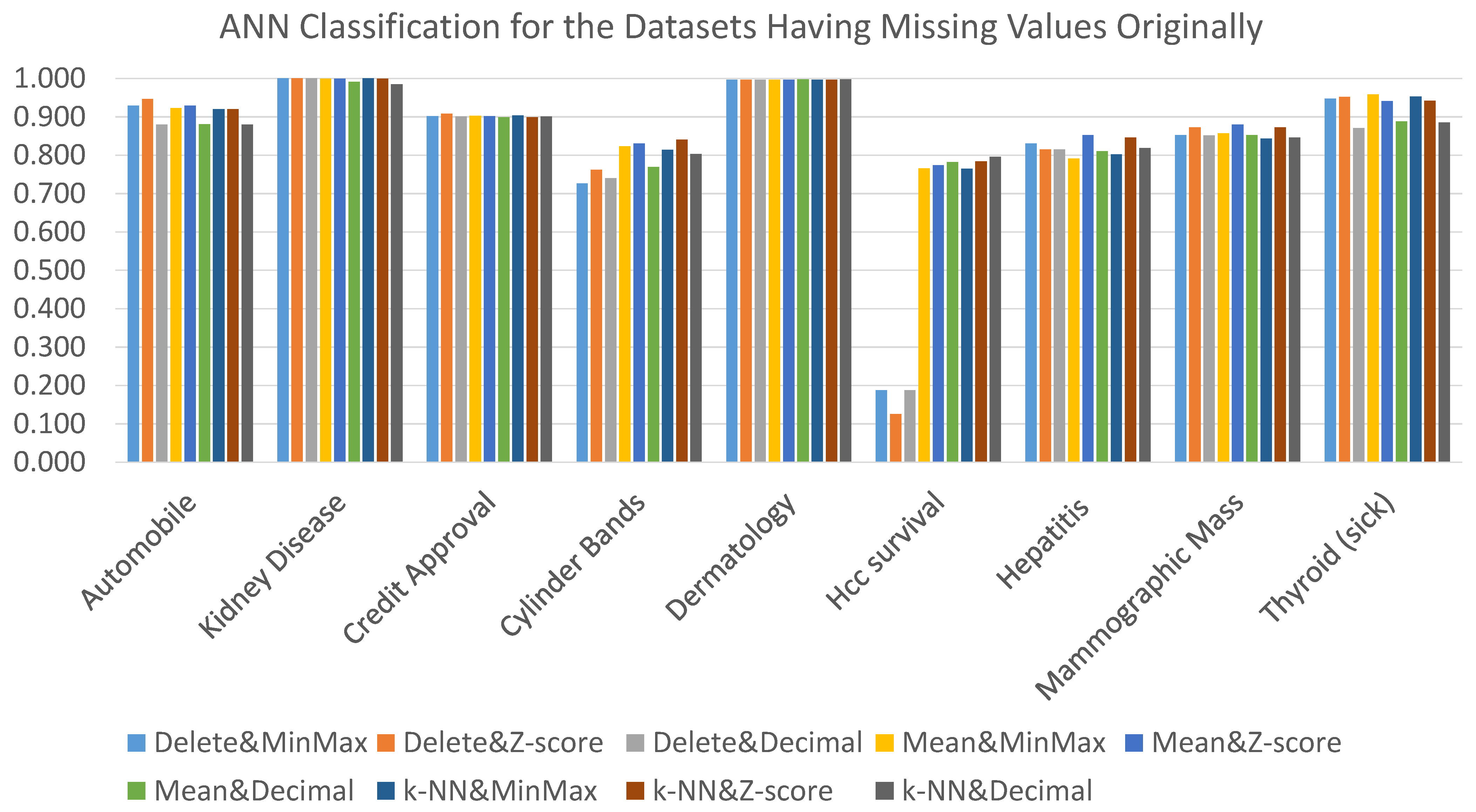
Thyroid	96.29	0.948	97.47	0.952	92.40	0.871	97.38	0.959	98.01	0.941	94.33	0.888	97.45	0.953	98.01	0.942	94.41	0.885

presents the results in terms of accuracy and AUC measures. As noted earlier, the discussion of the results will be based on the AUC measure. Thus, Figure 2 shows the results in terms of the AUC measure. From the figure, it can be clearly observed that no one data preprocessing technique outperforms the others for all datasets. In addition, it can be noted that for most datasets, the obtained results are close, except the HCC survival dataset, where the delete strategy significantly degrades the classification accuracy regardless of the adopted normalization technique, the reasons behind this being: (i) the high missing values rate compared to the remaining eight datasets (see Table 1) and (ii) the distribution of missing values in the dataset.

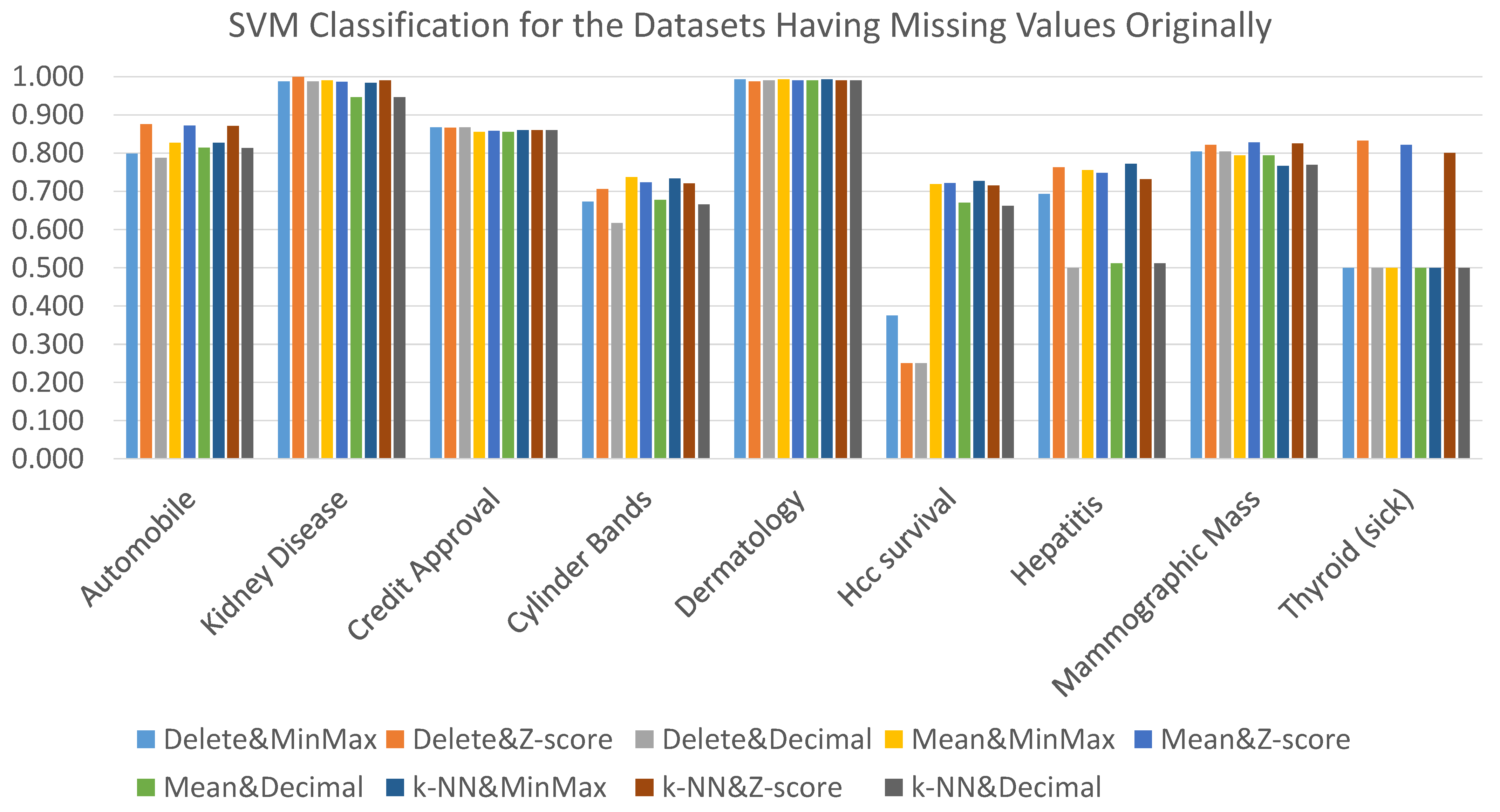
The results obtained when using the SVM classification algorithm coupled with the nine alternative data preprocessing combination techniques are presented in Figure 3, and the detailed results are tabulated in

Table A2. Average accuracy and AUC values obtained using the SVM classification algorithm coupled with the nine data preprocessing techniques with respect to the datasets that featured missing values originally.

	SVM Classification
Technique	$\mathit{Delete}\&$		$\mathit{Delete}\&$		$\mathit{Delete}\&$		$\mathit{Mean}\&$		$\mathit{Mean}\&$		$\mathit{Mean}\&$		$\mathit{kNN}\&$		$\mathit{kNN}\&$		$\mathit{kNN}\&$
	$\mathit{MinMax}$		$\mathit{Zscore}$		$\mathit{Decimal}$		$\mathit{MinMax}$		$\mathit{Zscore}$		$\mathit{Decimal}$		$\mathit{MinMax}$		$\mathit{Zscore}$		$\mathit{Decimal}$
Dataset	Acc.	AUC	Acc.	AUC	Acc.	AUC	Acc.	AUC	Acc.	AUC	Acc.	AUC	Acc.	AUC	Acc.	AUC	Acc.	AUC
Automobile	64.15	0.799	74.84	0.876	64.15	0.788	68.29	0.827	76.59	0.872	64.88	0.814	67.80	0.827	77.07	0.871	64.88	0.813
Kidney	99.37	0.988	100.00	1.000	99.36	0.988	98.75	0.990	98.50	0.987	93.25	0.946	98.00	0.984	98.75	0.990	93.25	0.946
Credit	86.22	0.868	86.06	0.867	86.22	0.868	84.93	0.856	85.07	0.858	84.93	0.856	85.22	0.860	85.22	0.860	85.22	0.860
Cylinder	71.48	0.673	74.01	0.706	66.07	0.617	75.19	0.737	73.89	0.724	69.63	0.678	75.37	0.734	73.89	0.721	68.52	0.666
Dermatology	97.77	0.993	96.09	0.988	96.93	0.990	97.54	0.993	96.72	0.990	96.99	0.990	97.54	0.993	96.72	0.990	96.99	0.990
HCC survival	37.50	0.375	25.00	0.250	25.00	0.250	73.94	0.719	73.94	0.722	72.73	0.670	74.55	0.727	73.33	0.715	72.12	0.662
Hepatitis	85.00	0.693	86.25	0.763	83.75	0.500	85.16	0.756	83.87	0.748	79.35	0.512	85.81	0.772	83.23	0.732	79.35	0.512
Mammographic	80.24	0.804	82.17	0.822	80.24	0.804	79.08	0.794	82.83	0.828	79.08	0.794	76.90	0.767	82.52	0.825	77.11	0.769
Thyroid	91.98	0.500	96.22	0.833	91.98	0.500	93.88	0.500	97.06	0.822	93.88	0.500	93.88	0.500	96.90	0.801	93.88	0.500

. From the figure, we can observe the significant impact of the adopted preprocessing technique on the classification accuracy with respect to some datasets, such as the case of the Thyroid dataset where the obtained AUC results range from 0.500 to 0.833. Another case is the Hepatitis dataset, where the obtained AUC range was [0.500–0.772]. With respect to the HCC survival dataset, the same as using the ANN classifier, the delete strategy produced the worst AUC results regardless of the adopted normalization technique.

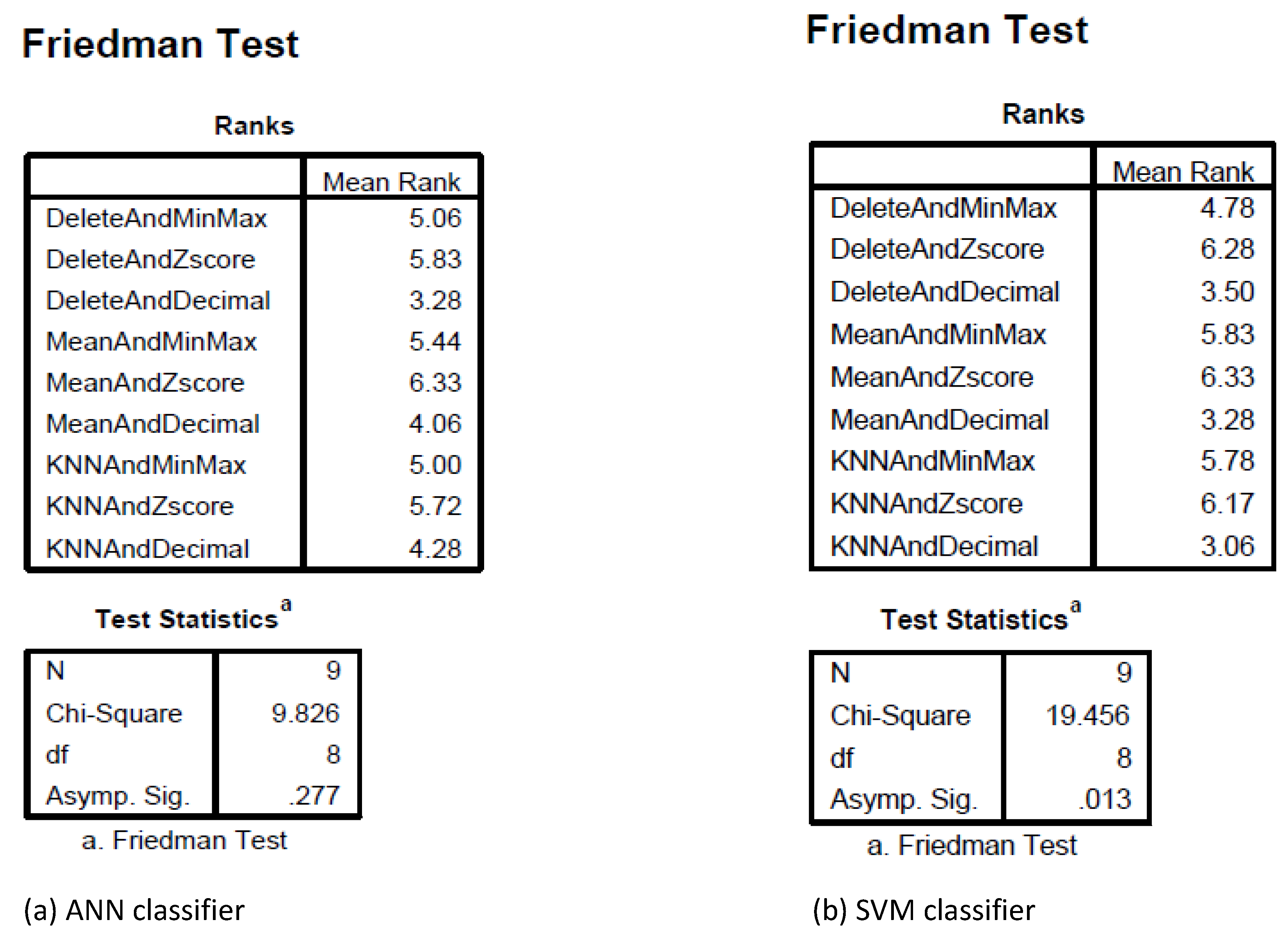
In order to achieve a more precise evaluation of the effect of different preprocessing combination techniques on classification effectiveness, statistical tests were applied. Regarding the statistical comparison of the nine considered data preprocessing combination techniques coupled with the ANN classifier, the Friedman test was applied. Figure 4a shows the reported Friedman test results using SPSS. The Friedman test reported that there was no significant difference between the nine data preprocessing techniques ($X^2\left(2\right)$ = 9.826, p = 0.277). With respect to comparing the nine data preprocessing combination techniques and SVM classifier, the Friedman test reported a significant difference between the nine data preprocessing techniques ($X^2\left(2\right)$ = 19.456, p = 0.013), as shown in Figure 4b. Consequently, the Nemenyi post-hoc test was applied to determine the data preprocessing combination technique that significantly outperformed the others. When applying the Nemenyi post-hoc test, two models are significantly different if the difference of their mean rank is higher than or equal to the Critical Difference (CD) [13]. The CD is calculated according to the following Equation [37].

$$CD=q_{\alpha }\sqrt{\frac{k\left(k+1\right)}{6N}}$$

(4)

where $q_{\alpha }$ is the confidence level, k is the number of models, and N is the number of datasets.

With respect to our comparison, k = 9, N = 9, and $\alpha$ = 0.05 were adopted. Thus, $CD=3.102\sqrt{\frac{9\left(9+1\right)}{6\ast 9}}=4.005$. Then, the difference between the mean ranks manipulated for each pair of models (preprocessing combinations) is compared with the value of the critical difference. Because the difference between the highest mean rank and the lowest mean rank is less than the CD (6.33 − 3.06 = 3.27 < 4.005), the Nemenyi test did not detect any significant differences between the models.

5.2. Results Obtained from Datasets Having 10% Artificially Generated Missing Values

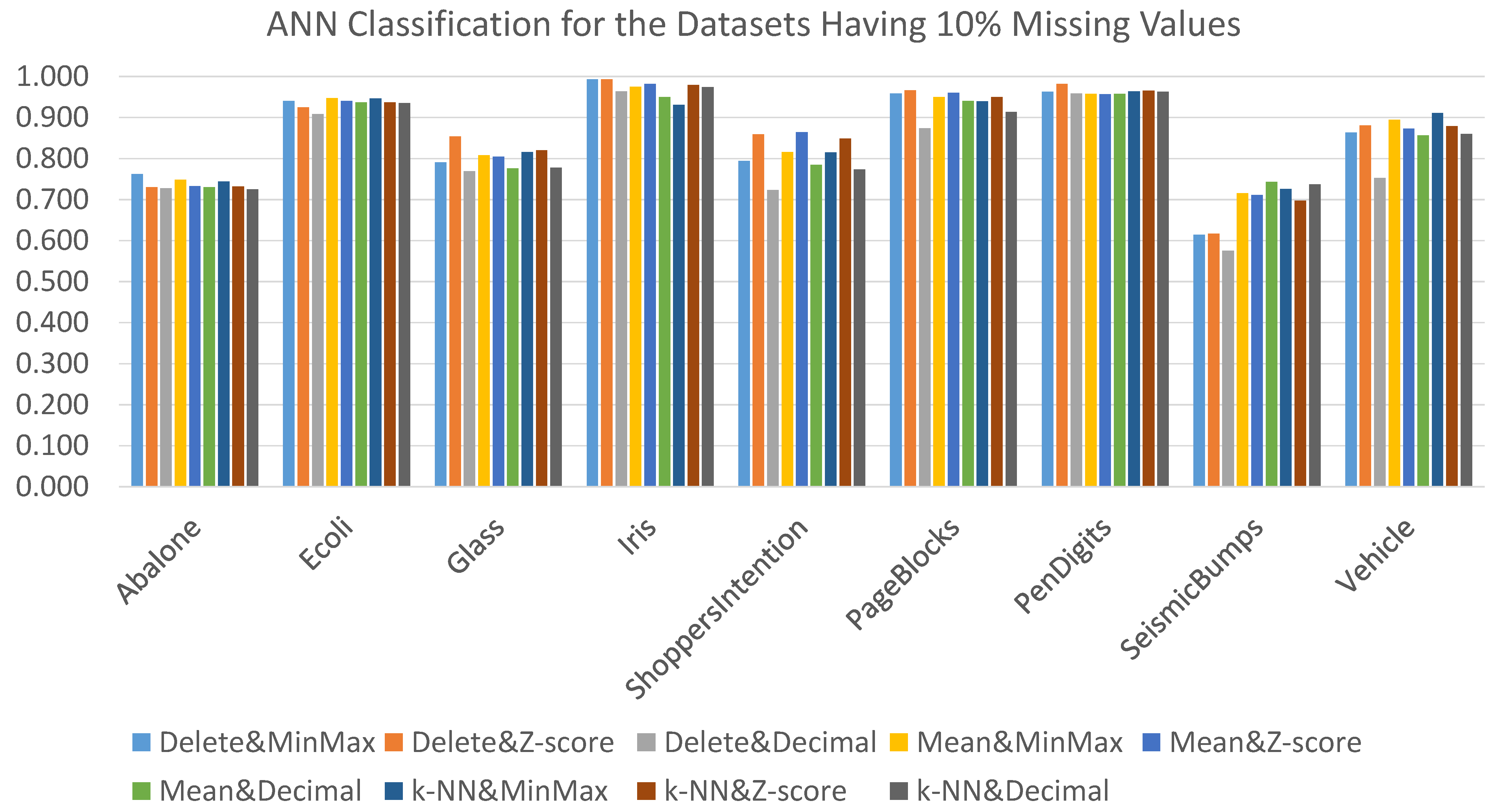
This section presents the results obtained when using the ANN and SVM classification algorithms coupled with the nine alternative data preprocessing combination techniques for datasets with a 10% missing values rate (generated artificially). We commence with the results obtained when using the ANN classification algorithm presented in Figure 5, and

Table A3. Average accuracy and AUC values obtained using the ANN classification algorithm coupled with the nine data preprocessing techniques with respect to the datasets that feature 10% missing values.

	ANN Classification
Technique	$\mathit{Delete}\&$		$\mathit{Delete}\&$		$\mathit{Delete}\&$		$\mathit{Mean}\&$		$\mathit{Mean}\&$		$\mathit{Mean}\&$		$\mathit{kNN}\&$		$\mathit{kNN}\&$		$\mathit{kNN}\&$
	$\mathit{MinMax}$		$\mathit{Zscore}$		$\mathit{Decimal}$		$\mathit{MinMax}$		$\mathit{Zscore}$		$\mathit{Decimal}$		$\mathit{MinMax}$		$\mathit{Zscore}$		$\mathit{Decimal}$
Dataset	Acc.	AUC	Acc.	AUC	Acc.	AUC	Acc.	AUC	Acc.	AUC	Acc.	AUC	Acc.	AUC	Acc.	AUC	Acc.	AUC
Abalone	26.69	0.762	25.10	0.730	25.20	0.728	25.54	0.748	25.64	0.733	25.14	0.730	26.09	0.744	25.16	0.732	25.13	0.725
Ecoli	82.10	0.940	77.78	0.925	76.54	0.908	84.23	0.947	79.46	0.940	78.27	0.937	83.93	0.946	79.17	0.937	78.27	0.935
Glass	63.10	0.791	70.24	0.854	55.95	0.769	59.81	0.808	63.08	0.804	55.14	0.776	61.22	0.816	62.15	0.820	54.21	0.778
Iris	92.55	0.993	93.62	0.993	91.49	0.964	90.67	0.975	93.33	0.982	86.67	0.950	86.67	0.931	92.67	0.979	89.33	0.974
ShopperIntention	84.29	0.794	86.77	0.859	82.13	0.723	85.49	0.816	86.85	0.864	84.28	0.785	84.89	0.815	85.36	0.849	84.01	0.773
PageBlocks	96.54	0.959	96.32	0.966	93.61	0.874	95.45	0.950	95.78	0.960	94.66	0.940	94.81	0.939	95.38	0.950	94.13	0.913
PenDigits	93.42	0.963	95.33	0.982	92.37	0.959	89.92	0.958	89.74	0.957	90.57	0.958	91.64	0.964	91.23	0.965	92.29	0.963
SeismicBumps	92.11	0.614	90.79	0.617	93.42	0.575	92.92	0.715	90.83	0.711	93.00	0.743	93.03	0.726	91.87	0.697	93.11	0.737
Vehicle	72.13	0.863	72.13	0.881	51.64	0.753	71.63	0.895	70.09	0.873	62.29	0.856	73.29	0.911	70.92	0.879	63.71	0.861

presents the detailed results. From the figure, it can be seen that Delete&Zscore produced the best AUC results for three datasets, Delete&MinMax generated the best AUC for one dataset, Mean&MinMax generated the best AUC for one dataset, Mean&MinMax generated the best AUC for one dataset, Mean&Zscore generated the best AUC for one dataset, Mean&Decimal generated the best AUC for one dataset, and kNN&MinMax generated the best AUC for one dataset. For one dataset, the same AUC results were obtained regardless of the adopted data preprocessing combination technique. It is interesting to note here that SeismicBumps was highly affected by the adopted preprocessing combination technique where the AUC range was [0.575–0.743]. Note here that the AUC value 0.575 was obtained when applying the Delete&Decimal preprocessing combination technique.

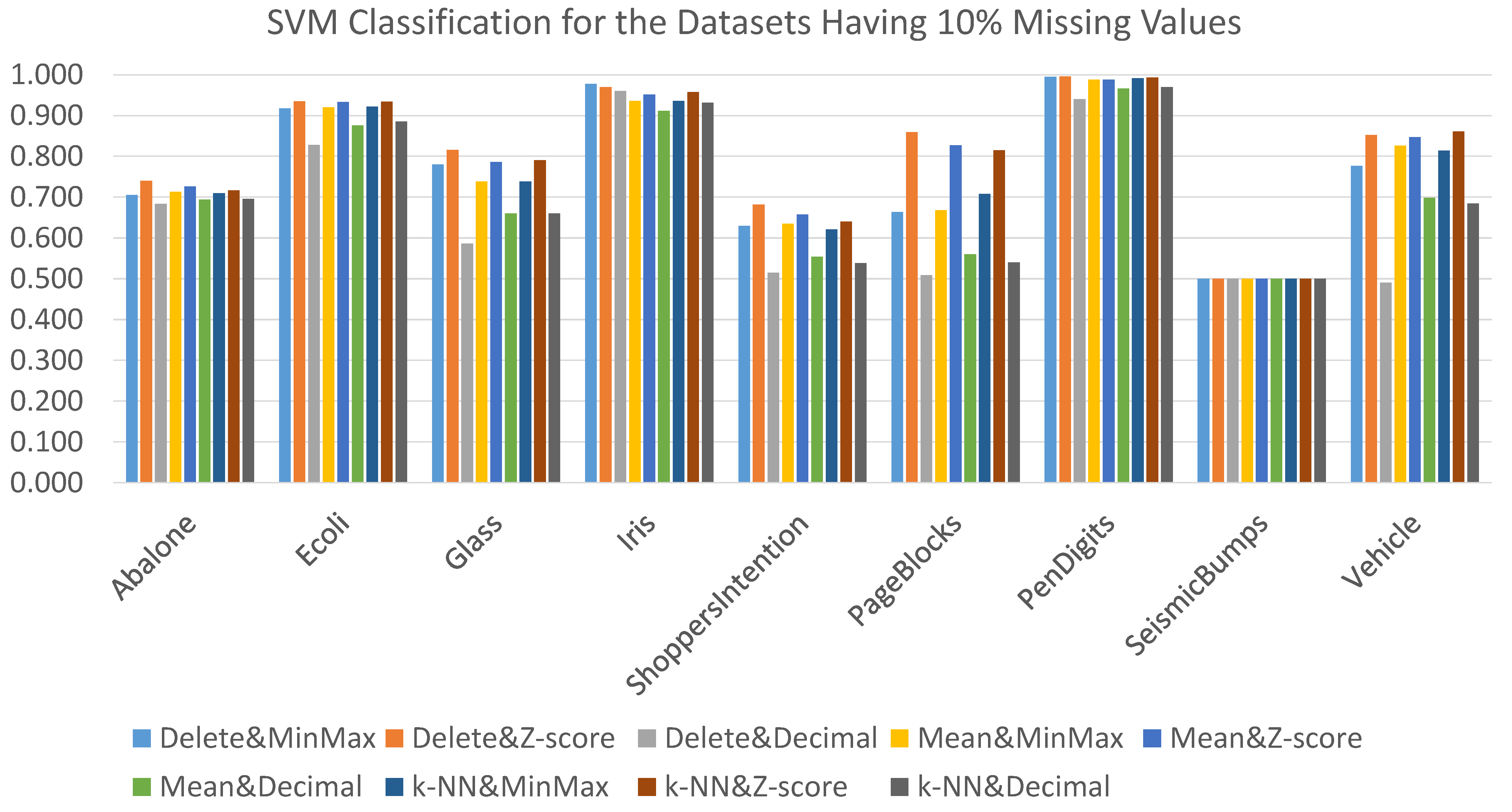
Figure 6 displays the results using the nine data preprocessing combination techniques coupled with the SVM classification algorithm in the context of a 10% missing values rate. From the figure, it can be noted that Delete&Zscore produced the best AUC results for most datasets. More specifically, Delete&Zscore produced the best AUC results for six datasets, while Delete &MinMax generated the best AUC for one dataset, and kNN &Zscore generated the best AUC for one dataset. For the remaining dataset (SeismicBumps), the same AUC results were obtained regardless of the adopted data preprocessing combination technique. Note here that the detailed results are presented in

Table A4. Average accuracy and AUC values obtained using the SVM classification algorithm coupled with the nine data preprocessing techniques with respect to the datasets that feature 10% missing values.

	SVM Classification
Technique	$\mathit{Delete}\&$		$\mathit{Delete}\&$		$\mathit{Delete}\&$		$\mathit{Mean}\&$		$\mathit{Mean}\&$		$\mathit{Mean}\&$		$\mathit{kNN}\&$		$\mathit{kNN}\&$		$\mathit{kNN}\&$
	$\mathit{MinMax}$		$\mathit{Zscore}$		$\mathit{Decimal}$		$\mathit{MinMax}$		$\mathit{Zscore}$		$\mathit{Decimal}$		$\mathit{MinMax}$		$\mathit{Zscore}$		$\mathit{Decimal}$
Dataset	Acc.	AUC	Acc.	AUC	Acc.	AUC	Acc.	AUC	Acc.	AUC	Acc.	AUC	Acc.	AUC	Acc.	AUC	Acc.	AUC
Abalone	23.21	0.705	25.51	0.740	22.85	0.683	24.01	0.713	25.66	0.726	22.50	0.694	23.38	0.709	24.22	0.716	22.69	0.696
Ecoli	75.93	0.918	84.57	0.935	62.96	0.828	79.46	0.920	82.74	0.933	73.21	0.876	79.76	0.922	83.33	0.934	74.11	0.885
Glass	61.90	0.780	67.86	0.816	40.48	0.586	56.07	0.738	59.81	0.786	43.93	0.660	56.07	0.738	61.22	0.790	43.93	0.660
Iris	95.74	0.977	95.74	0.970	92.55	0.960	88.67	0.936	92.00	0.951	86.00	0.911	88.67	0.936	93.33	0.957	85.33	0.931
ShopperIntention	87.44	0.630	88.29	0.682	84.76	0.515	87.70	0.635	88.05	0.657	85.90	0.554	87.40	0.621	87.62	0.640	85.48	0.538
PageBlocks	93.34	0.663	96.00	0.859	91.02	0.509	92.38	0.668	95.29	0.827	90.90	0.560	92.67	0.708	94.88	0.815	90.55	0.540
PenDigits	97.00	0.995	97.71	0.996	79.22	0.940	92.53	0.988	92.26	0.988	84.69	0.966	94.92	0.992	95.06	0.993	85.52	0.970
SeismicBumps	94.30	0.500	94.30	0.500	94.30	0.500	93.42	0.500	93.42	0.500	93.42	0.500	93.42	0.500	93.42	0.500	93.42	0.500
Vehicle	63.11	0.777	72.95	0.852	28.69	0.490	67.26	0.826	70.80	0.847	43.74	0.698	69.86	0.814	73.17	0.861	42.55	0.684

.

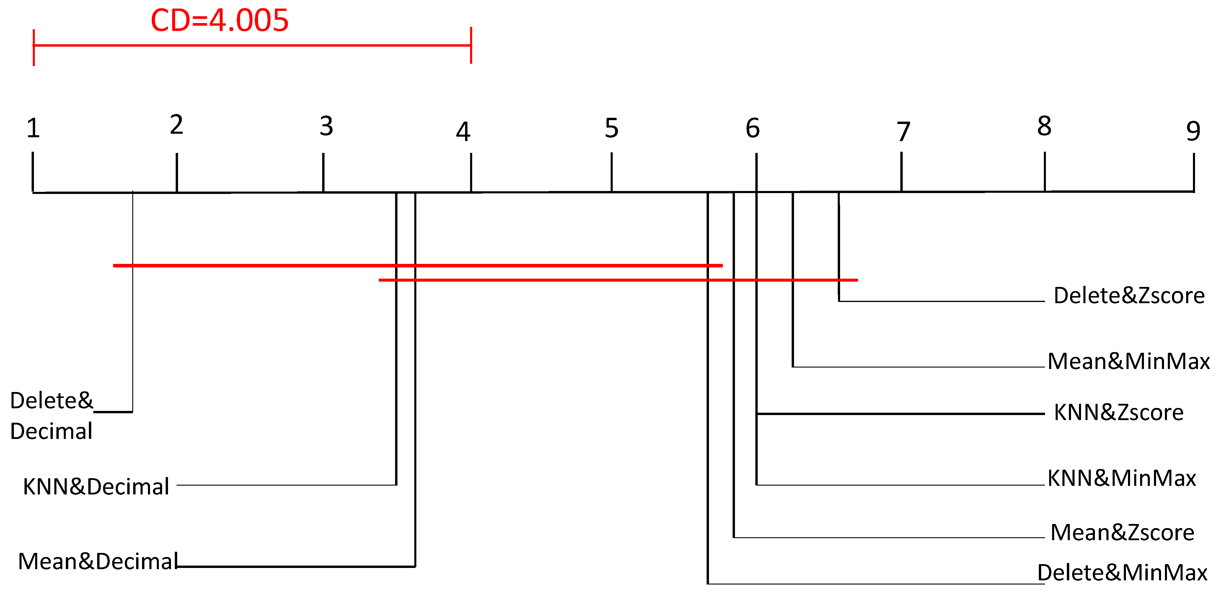
Regarding the statistical comparison of the nine considered data preprocessing combination techniques coupled with the ANN classifier, the Friedman test was applied. The Friedman test demonstrated that there was a significant difference between the nine data preprocessing techniques ($X^2\left(2\right)$ = 26.900, p = 0.001). As a result, the Nemenyi post-hoc test was applied to determine the data preprocessing combination technique that significantly outperformed the others. Note that k = 9, N = 9, and $\alpha$ = 0.05; thus, CD ≈ 4.005 was adopted. Figure 7 presents a visual representation of the Nemenyi test, where the mean ranks of all considered method are plotted (mean ranks were reported by the Friedman test using SPSS, where the highest mean rank was assigned to the best method). The models that are not significantly different are connected. Note here that the best model is positioned on the right. Interestingly, the Nemenyi test noted that Delete&Zscore, Mean&MinMax, Mean&Zscore, kNN&MinMax, and kNN&Zscore significantly outperformed Delete&Decimal. In other words, the statistical test result indicated that decimal normalization was the least effective normalization technique regardless of the coupled missing values treatment strategy. In addition, the worst combination technique was Delete&Decimal.

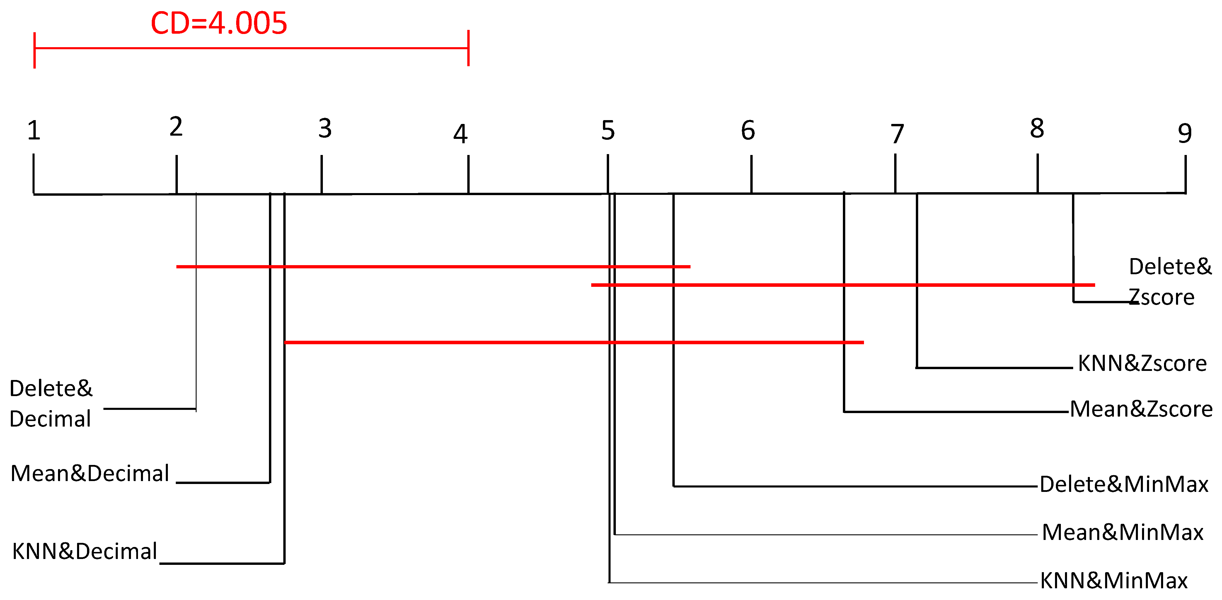
With respect to comparing the nine data preprocessing combination techniques and the SVM classifier, the Friedman test reported a significant difference between the nine data preprocessing techniques ($X^2\left(2\right)$ = 50.979, p = 0.000). Again, the Nemenyi post-hoc test was conducted to determine the data preprocessing combination technique that significantly outperformed the others. Figure 8 presents the visual representation of the Nemenyi test. As shown in the figure, the Nemenyi post-hoc noted that: (i) Delete&Zscore, Mean&Zscore, and kNN&Zscore significantly outperformed Delete&Decimal and Mean&Decimal, and (ii) Delete&Zscore and kNN&Zscore significantly outperformed kNN&Decimal. Again, Decimal normalization was the least effective normalization technique. In addition, Z-score normalization was the most effective normalization technique regardless of the coupled missing values treatment strategy.

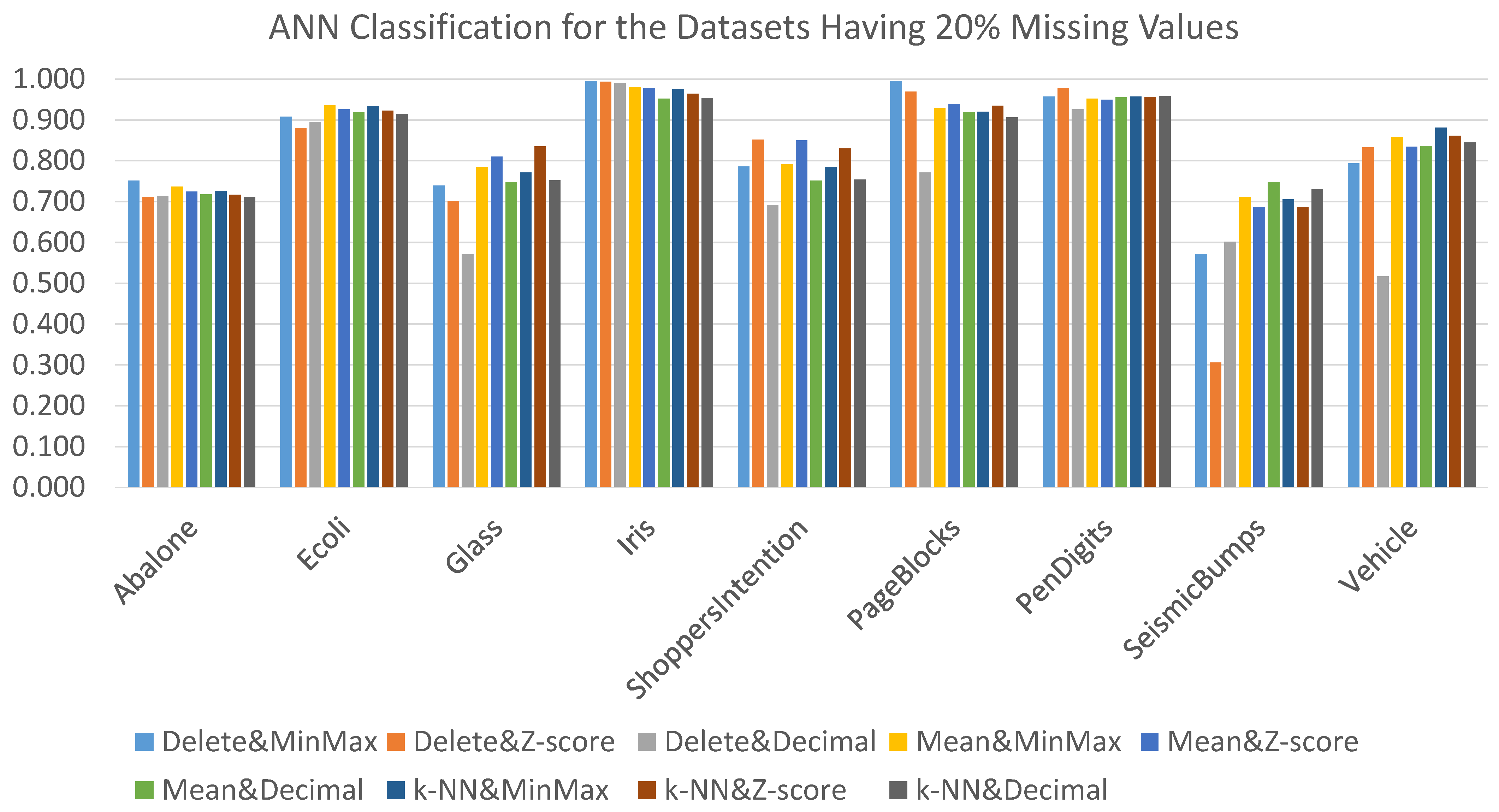
5.3. Results Obtained from Datasets Having 20% Artificially Generated Missing Values

The results obtained when using ANN classification algorithm coupled with the nine alternative data preprocessing combination techniques for datasets with 20% missing values are displaced in Figure 9. An interesting observation is that the delete strategy was working “good” even with 20% missing values compared to other missing values treatment strategies. More specifically, Delete&MinMax produced the best AUC results for three datasets, and Delete&Zscore produced the best AUC results for two datasets. For the remaining datasets, Mean&MinMax generated the best AUC for one dataset; Mean&Decimal generated the best AUC for one dataset; kNN&MinMax generated the best AUC for one dataset; and kNN&Zscore generated the best AUC for one dataset. The detailed results are presented in

Table A5. Average accuracy and AUC values obtained using the ANN classification algorithm coupled with the nine data preprocessing techniques with respect to the datasets that feature 20% missing values.

	ANN Classification
Technique	$\mathit{Delete}\&$		$\mathit{Delete}\&$		$\mathit{Delete}\&$		$\mathit{Mean}\&$		$\mathit{Mean}\&$		$\mathit{Mean}\&$		$\mathit{kNN}\&$		$\mathit{kNN}\&$		$\mathit{kNN}\&$
	$\mathit{MinMax}$		$\mathit{Zscore}$		$\mathit{Decimal}$		$\mathit{MinMax}$		$\mathit{Zscore}$		$\mathit{Decimal}$		$\mathit{MinMax}$		$\mathit{Zscore}$		$\mathit{Decimal}$
Dataset	Acc.	AUC	Acc.	AUC	Acc.	AUC	Acc.	AUC	Acc.	AUC	Acc.	AUC	Acc.	AUC	Acc.	AUC	Acc.	AUC
Abalone	26.34	0.751	25.06	0.712	25.17	0.714	24.30	0.737	24.01	0.724	25.23	0.718	25.08	0.726	24.92	0.717	23.58	0.712
Ecoli	78.67	0.908	69.33	0.880	78.67	0.895	81.25	0.936	76.79	0.926	75.30	0.918	80.65	0.934	78.27	0.922	75.89	0.915
Glass	59.26	0.739	51.85	0.700	40.74	0.570	59.35	0.784	60.75	0.810	52.34	0.748	59.81	0.771	66.36	0.835	54.67	0.752
Iris	94.34	0.995	94.34	0.994	92.45	0.990	92.00	0.980	90.00	0.978	84.67	0.952	93.33	0.975	92.67	0.964	84.00	0.954
ShopperIntention	84.87	0.786	86.66	0.852	80.18	0.692	84.61	0.791	86.24	0.850	82.90	0.751	84.04	0.785	84.87	0.830	83.42	0.754
PageBlocks	95.19	0.995	94.69	0.969	92.37	0.771	94.28	0.929	95.05	0.939	93.88	0.919	94.10	0.920	94.72	0.935	93.90	0.906
PenDigits	88.32	0.957	90.42	0.978	84.73	0.926	86.91	0.952	85.55	0.949	87.47	0.955	88.33	0.957	88.05	0.956	89.15	0.958
SeismicBumps	88.68	0.571	88.68	0.306	90.57	0.602	92.76	0.712	91.87	0.686	93.03	0.748	92.88	0.705	91.02	0.686	93.11	0.729
Vehicle	59.09	0.794	59.09	0.833	40.91	0.517	66.90	0.859	64.42	0.834	58.75	0.836	68.91	0.881	66.90	0.861	61.23	0.845

.

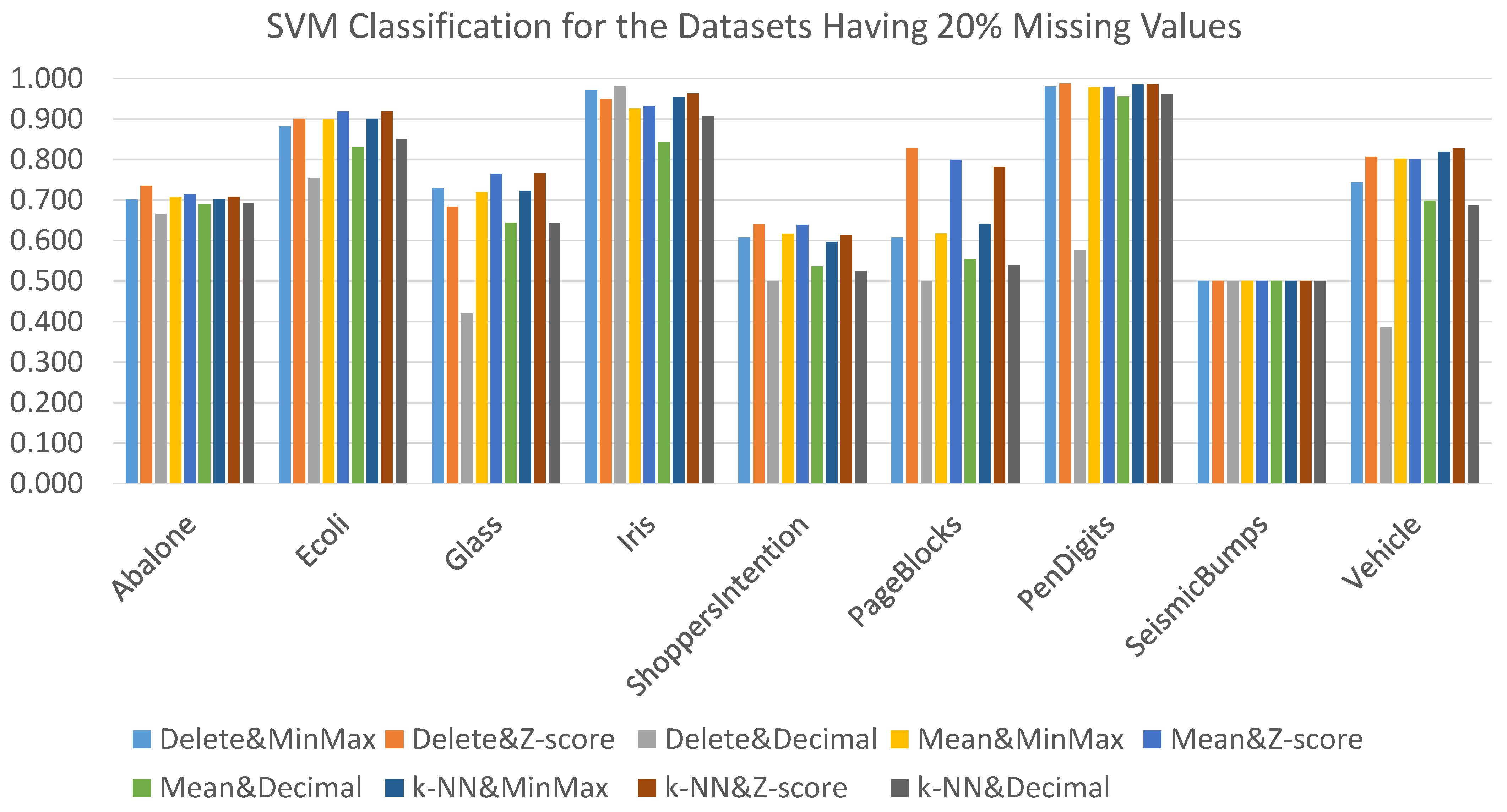
The results obtained when using the SVM classification algorithm coupled with the nine alternative data preprocessing combination techniques for datasets having 20% missing values are presented in Figure 10. The same as the case of the ANN classifier, the delete strategy was working “well” even with 20% missing values compared to other missing values treatment strategies. In addition, the Z-score technique generated the best AUC results for most cases regardless of the adopted treatment for missing values. More specifically, Delete&Zscore produced the best AUC results for four datasets, and kNN&Zscore produced the best AUC results for three datasets. For the remaining two datasets, Delete&Decimal generated the best AUC for one dataset, and all techniques generated the same AUC result for one dataset (SeismicBumps). The detailed results are presented in

Table A6. Average accuracy and AUC values obtained using the SVM classification algorithm coupled with the nine data preprocessing techniques with respect to the datasets that feature 20% missing values.

	SVM Classification
Technique	$\mathit{Delete}\&$		$\mathit{Delete}\&$		$\mathit{Delete}\&$		$\mathit{Mean}\&$		$\mathit{Mean}\&$		$\mathit{Mean}\&$		$\mathit{kNN}\&$		$\mathit{kNN}\&$		$\mathit{kNN}\&$
	$\mathit{MinMax}$		$\mathit{Zscore}$		$\mathit{Decimal}$		$\mathit{MinMax}$		$\mathit{Zscore}$		$\mathit{Decimal}$		$\mathit{MinMax}$		$\mathit{Zscore}$		$\mathit{Decimal}$
Dataset	Acc.	AUC	Acc.	AUC	Acc.	AUC	Acc.	AUC	Acc.	AUC	Acc.	AUC	Acc.	AUC	Acc.	AUC	Acc.	AUC
Abalone	22.49	0.701	24.13	0.735	22.03	0.666	23.17	0.707	24.16	0.714	22.15	0.689	22.93	0.703	23.91	0.708	22.33	0.692
Ecoli	66.67	0.882	77.33	0.900	50.67	0.755	76.79	0.899	80.06	0.918	67.86	0.831	77.68	0.900	80.36	0.919	70.24	0.851
Glass	62.96	0.729	55.56	0.684	40.74	0.420	54.67	0.720	56.54	0.765	43.46	0.644	55.61	0.723	57.48	0.766	42.99	0.643
Iris	94.34	0.971	55.56	0.949	96.23	0.981	86.00	0.927	88.00	0.932	76.00	0.843	92.00	0.955	94.00	0.963	83.33	0.907
ShopperIntention	87.56	0.607	87.18	0.640	84.95	0.500	87.34	0.617	87.73	0.639	85.46	0.537	86.87	0.597	87.22	0.614	85.20	0.525
PageBlocks	91.54	0.607	94.69	0.829	90.05	0.500	91.72	0.618	94.63	0.799	90.77	0.554	92.02	0.641	94.24	0.782	90.48	0.538
PenDigits	91.32	0.981	95.81	0.988	13.47	0.577	87.88	0.979	87.89	0.980	80.90	0.956	90.91	0.985	91.27	0.986	82.68	0.962
SeismicBumps	92.45	0.500	92.45	0.500	92.45	0.500	93.42	0.500	93.42	0.500	93.42	0.500	93.42	0.500	93.42	0.500	93.42	0.500
Vehicle	59.09	0.744	68.18	0.807	22.73	0.386	62.06	0.802	61.70	0.801	45.98	0.699	64.54	0.820	66.19	0.828	44.44	0.688

.

Regarding the statistical comparison of the nine considered data preprocessing combination techniques coupled with the ANN classifier, the Friedman test was applied. The Friedman test demonstrated that there was a significant difference between the nine data preprocessing techniques ($X^2\left(2\right)$ = 16.052, p = 0.042). Applying the Nemenyi post-hoc test, the only reported significant difference was between Mean&MinMax and Delete&Decimal, where the Mean&MinMax technique significantly outperformed Delete&Decimal, as shown in Figure 11.

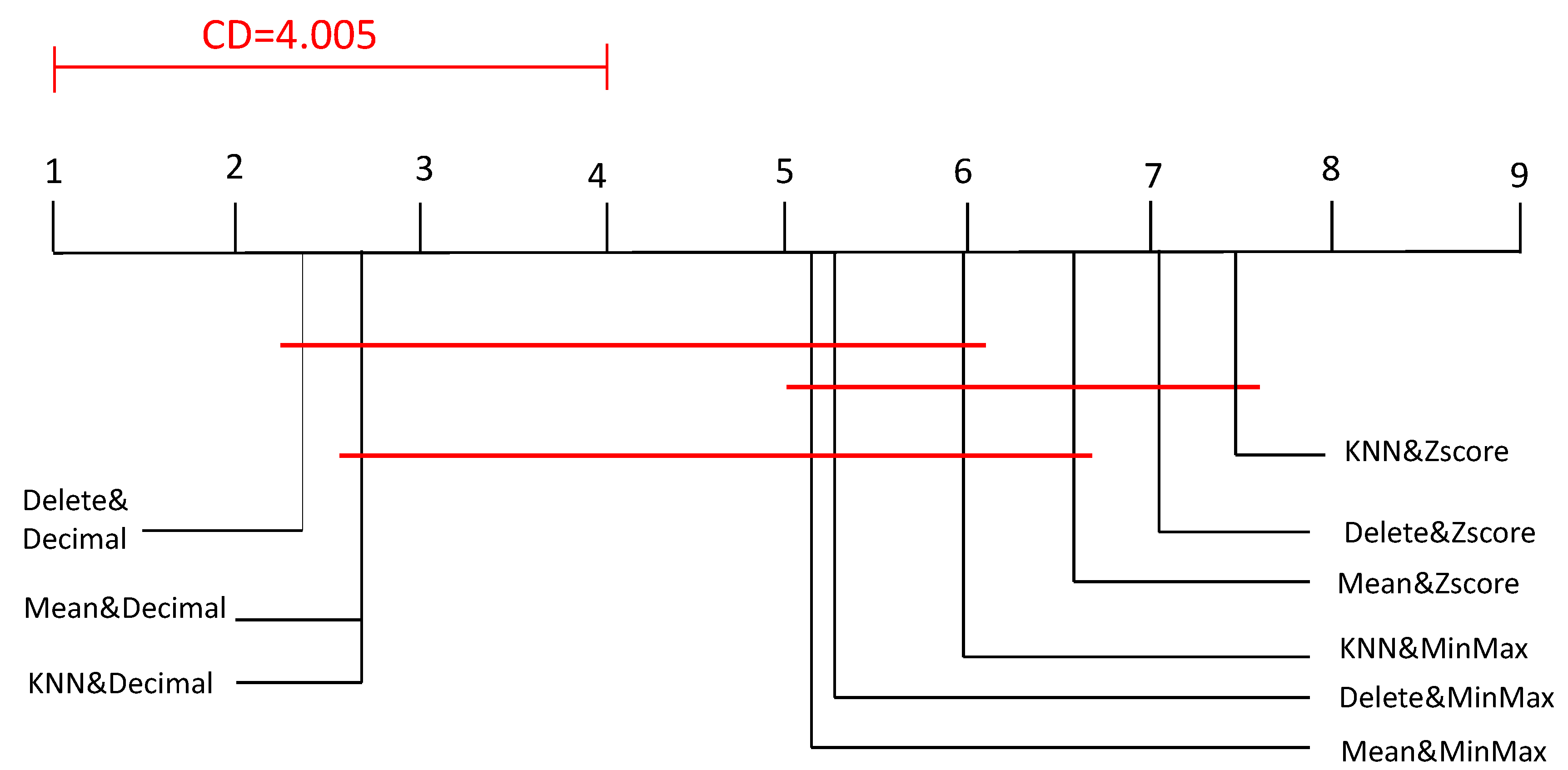
With respect to the statistical comparison of the nine considered data preprocessing combination techniques coupled with the SVM classifier, the Friedman test was applied. The Friedman test demonstrated that there was a significant difference between the nine data preprocessing techniques ($X^2\left(2\right)$ = 42.669, p = 0.000). The Nemenyi post-hoc test reported that: (i) Delete&Zscore, Mean&Zscore, and kNN&Zscore significantly outperformed Delete&Decimal, and (ii) Delete&Zscore and kNN&Zscore significantly outperformed Mean&Decimal and kNN&Decimal, as shown in Figure 12.

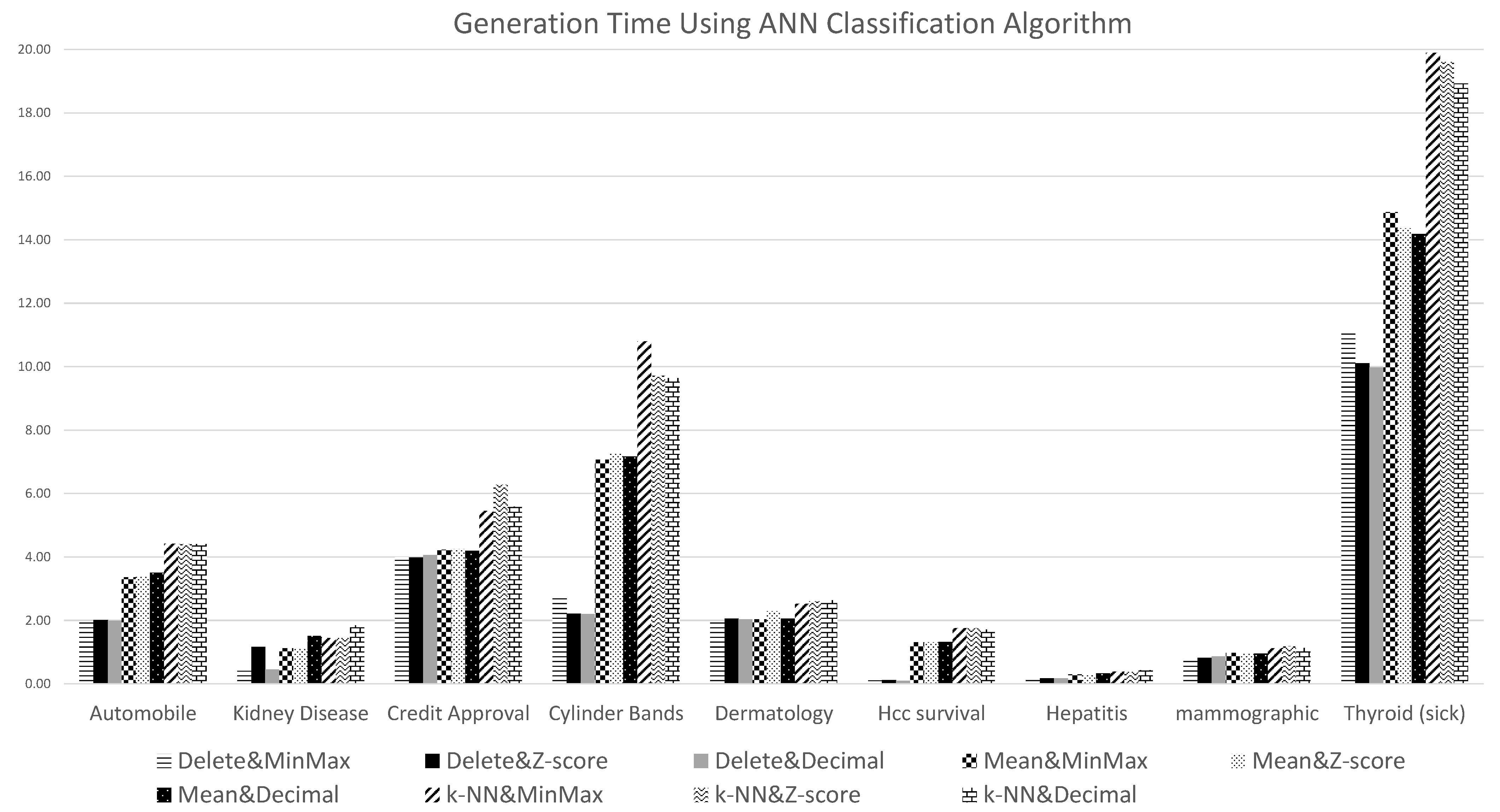
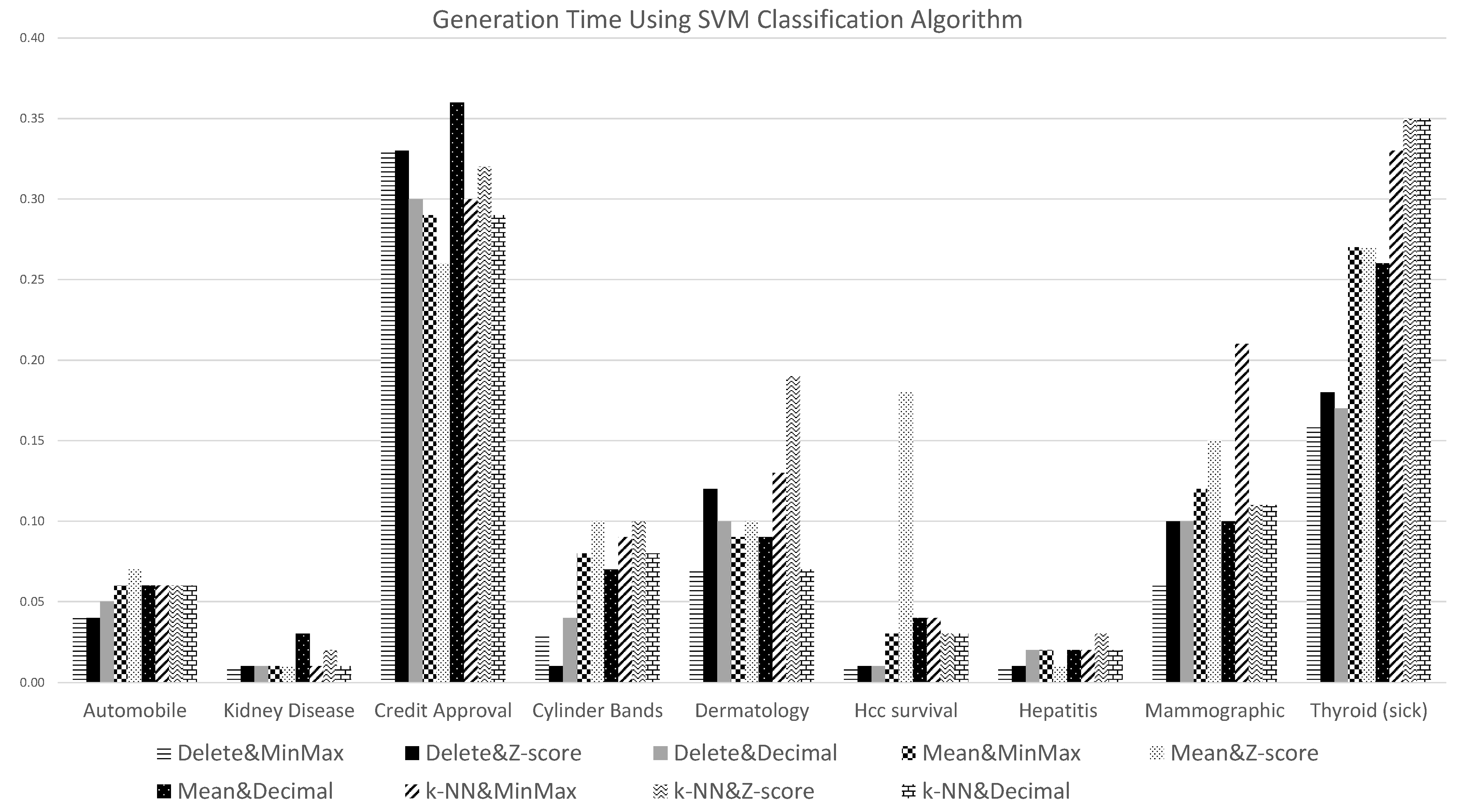
5.4. Classification Models Efficiency

The previous Section 5.1, Section 5.2 and Section 5.3 presented a comparison of the effectiveness of the nine considered data preprocessing combination techniques. In order to achieve a comprehensive comparison, this sub-section presents a comparison of the efficiency of the nine considered data preprocessing combination techniques. Figure 13 shows the generation time results (in seconds) obtained when using the ANN classification algorithm coupled with the nine data preprocessing combination techniques, and Figure 14 shows the generation time results (in seconds) obtained when using the SVM classification algorithm coupled with the nine data preprocessing combination techniques

Commencing with missing values treatment strategies, as expected, it can be noted that the lowest generation run times were obtained when using the delete strategy for handling missing values, and this is very obvious for datasets featuring high missing values rates; while the kNN technique for handling missing values generated the highest generation times. Additionally, it is interesting to note here that the effect of handling missing values on classification efficiency was more obvious when the ANN classification algorithm was adopted to generate the classification models. With respect to the data normalization techniques, there was no significant difference in efficiency between the three considered data normalization techniques.

6. Conclusions and Future Work

Handling missing values and data normalization are considered important preprocessing activities prior to applying classification algorithms. In this paper, the effect of different combinations of data preprocessing techniques was investigated. Three well-known normalization techniques and three well-known strategies for handling missing values were considered. Consequently, nine alternative data preprocessing combination techniques were evaluated: (i) Delete&MinMax combination technique, (ii) Delete&Z-score combination technique, (iii) Delete&Decimal combination technique, (iv) Mean&MinMax combination technique, (v) Mean&Z-score combination technique, (vi) Mean&Decimal combination technique, (vii) kNN&MinMax combination technique, (viii) kNN&Z-score combination technique, and (ix) kNN&Decimal combination technique. The classification models were generated using the ANN and SVM classification algorithms. Eighteen datasets were used to evaluate the nine data preprocessing combination techniques. The datasets were categorized into three categories according to the inclusion of missing values: (i) datasets having missing values originally, (ii) datasets having 10% missing values generated artificially, and (iii) datasets having 20% missing values generated artificially.

From the reported evaluation, there was no noticeable difference between the considered data preprocessing combination techniques with respect to most datasets that featured missing values originally. In other words, there was no significant effect of the adopted preprocessing techniques for most datasets having less than 10% missing values. Regarding datasets having 10% missing values, there was a significant effect of the adopted preprocessing techniques on the performance of classification models, the statistical tests results indicating that decimal normalization was the least effective normalization technique regardless of the coupled missing values treatment strategy, while Z-score normalization was the most effective normalization technique regardless of the coupled missing values treatment strategy. Moreover, the worst combination technique was Delete&Decimal.

In the context of datasets having 20% missing values, unexpectedly, the delete strategy worked very well compared to the considered missing values treatment strategies. Thus, we proved that the delete strategy can be adopted for datasets featuring up to 20% missing values and can produce comparable classification accuracy compared to the mean and kNN strategies. In addition, the same as the case of the datasets with 10% missing values, decimal normalization was the least effective normalization technique, while Z-score normalization tended to generate the best AUC results, and the worst preprocessing combination technique was Delete&Decimal.

Interestingly, the impact of the adopted preprocessing techniques varied from one classification algorithm to another. More specifically, the effect of the data preprocessing techniques was more noticeable when the SVM classifier was utilized to generate the classification models. Overall, for most scenarios, Delete&Decimal was the worst preprocessing combination technique that could be applied before generating the desired classification model.

As future work, the authors intend to investigate the impact of different preprocessing techniques on clustering algorithms. In addition, generating datasets with more than a 20% missing values rate will be considered in order to determine the best preprocessing techniques to be adopted for such datasets.

References

- Kuhn, M.; Johnson, K. Data Pre-processing. In Applied Predictive Modeling; Springer: New York, NY, USA, 2013; pp. 27–59. [Google Scholar] [CrossRef]
- Crone, S.; Lessmann, S.; Stahlbock, R. The impact of preprocessing on data mining: An evaluation of classifier sensitivity in direct marketing. Eur. J. Oper. Res. 2006, 173, 781–800. [Google Scholar] [CrossRef]
- KumarSingh, B.; Verma, K.; Thoke, A.S. Investigations on Impact of Feature Normalization Techniques on Classifier’s Performance in Breast Tumor Classification. Int. J. Comput. Appl. 2015, 116, 11–15. [Google Scholar] [CrossRef]
- Alizadeh Naeini, A.; Babadi, M.; Homayouni, S. Assessment of Normalization Techniques on the Accuracy of Hyperspectral Data Clustering. ISPRS Int. Arch. Photogramm. Remote Sens. Spat. Inf. Sci. 2017, XLII-4/W4, 27–30. [Google Scholar] [CrossRef] [Green Version]
- Jiawei, H.; Micheline, K.; Jian, P. Data Mining: Concepts and Techniques; Morgan Kaufmann: San Mateo, CA, USA, 2011. [Google Scholar]
- Jayalskshmi, T.; Santhakumaran, A. Impact of Preprocessing for Diagnosis of Diabetes Mellitus Using Artificial Neural Networks. In Proceedings of the 2010 Second International Conference on Machine Learning and Computing, Bangalore, India, 12–13 February 2010; pp. 109–112. [Google Scholar] [CrossRef]
- Huang, H.C.; Qin, L.X. Empirical evaluation of data normalization methods for molecular classification. PeerJ 2018, 6, e4584. [Google Scholar] [CrossRef] [PubMed] [Green Version]
- Rozenstein, O.; Paz Kagan, T.; Salbach, C.; Karnieli, A. Comparing the Effect of Preprocessing Transformations on Methods of Land-Use Classification Derived From Spectral Soil Measurements. IEEE J. Sel. Top. Appl. Earth Obs. Remote Sens. 2014, 1–12. [Google Scholar] [CrossRef]
- Baitharu, T.R.; Pani, S.K. Effect of Missing Values on Data Classification. J. Emerg. Trends Eng. Appl. Sci. (JETEAS) 2013, 4, 311–316. [Google Scholar]
- Olsen, I.; Kvien, T.; Uhlig, T. Consequences of handling missing data for treatment response in osteoarthritis: A simulation study. Osteoarthr. Cartil. 2012, 20, 822–828. [Google Scholar] [CrossRef] [Green Version]
- Hunt, L.A. Missing Data Imputation and Its Effect on the Accuracy of Classification; Data Science; Palumbo, F., Montanari, A., Vichi, M., Eds.; Springer International Publishing: Cham, Switzerland, 2017; pp. 3–14. [Google Scholar]
- Friedman, M. A Comparison of Alternative Tests of Significance for the Problem of m Rankings. Ann. Math. Stat. 1940, 11, 86–92. [Google Scholar] [CrossRef]
- Nemenyi, P. Distribution-Free Multiple Comparisons; Princeton University: Princeton, NJ, USA, 1963. [Google Scholar]
- Corizzo, R.; Ceci, M.; Japkowicz, N. Anomaly Detection and Repair for Accurate Predictions in Geo-distributed Big Data. Big Data Res. 2019, 16, 18–35. [Google Scholar] [CrossRef]
- Acuña, E.; Rodriguez, C. The Treatment of Missing Values and its Effect on Classifier Accuracy. In Classification, Clustering, and Data Mining Applications; Banks, D., McMorris, F.R., Arabie, P., Gaul, W., Eds.; Springer: Berlin/Heidelberg, Germany, 2004; pp. 639–647. [Google Scholar]
- Saar-Tsechansky, M.; Provost, F. Handling Missing Values when Applying Classification Models. J. Mach. Learn. Res. 2007, 8, 1623–1657. [Google Scholar]
- GarcíA-Laencina, P.J.; Sancho-GóMez, J.L.; Figueiras-Vidal, A.R. Pattern Classification with Missing Data: A Review. Neural Comput. Appl. 2010, 19, 263–282. [Google Scholar] [CrossRef]
- Osborne, J. Best Practices in Data Cleaning: A Complete Guide to Everything You Need to Do before and after Collecting Your Data; SAGE: Thousand Oaks, CA, USA, 2013. [Google Scholar]
- Purwar, A.; Singh, S.K. Hybrid prediction model with missing value imputation for medical data. Expert Syst. Appl. 2015, 42, 5621–5631. [Google Scholar] [CrossRef]
- Luengo, J.; García, S.; Herrera, F. On the choice of the best imputation methods for missing values considering three groups of classification methods. Knowl. Inf. Syst. 2012, 32, 77–108. [Google Scholar] [CrossRef]
- Qie, Y.; Song, P.; Hao, C. Data Repair Without Prior Knowledge Using Deep Convolutional Neural Networks. IEEE Access 2020, 8, 105351–105361. [Google Scholar] [CrossRef]
- Foody, G.M.; Arora, M.K. An evaluation of some factors affecting the accuracy of classification by an artificial neural network. Int. J. Remote Sens. 1997, 18, 799–810. [Google Scholar] [CrossRef]
- Eftekhary, M.; Gholami, P.; Safari, S.; Shojaee, M. Ranking Normalization Methods for Improving the Accuracy of SVM Algorithm by DEA Method. Mod. Appl. Sci. 2012, 6, 26–36. [Google Scholar] [CrossRef] [Green Version]
- Wohlrab, L.; Fürnkranz, J. A Comparison of Strategies for Handling Missing Values in Rule Learning; Technical Report; Knowledge Engineering Group, Technische Universität Darmstadt: Darmstadt, Germany, 2009. [Google Scholar]
- Almuhaideb, S.; Menai, M.E.B. Impact of preprocessing on medical data classification. Front. Comput. Sci. 2016, 10, 1082–1102. [Google Scholar] [CrossRef]
- Jordanov, I.; Petrov, N.; Petrozziello, A. Classifiers accuracy improvement based on missing data imputation. J. Artif. Intell. Soft Comput. Res. 2018, 8, 31–48. [Google Scholar] [CrossRef] [Green Version]
- Peugh, J.; Enders, C. Missing Data in Educational Research: A Review of Reporting Practices and Suggestions for Improvement. Rev. Educ. Res. 2004, 74, 525–556. [Google Scholar] [CrossRef]
- Aleryani, A.; Wang, W.; De La Iglesia, B. Dealing with Missing Data and Uncertainty in the Context of Data Mining. In Hybrid Artificial Intelligent Systems; Springer: Berlin/Heidelberg, Germany, 2018; pp. 289–301. [Google Scholar] [CrossRef] [Green Version]
- Kim, T.; Ko, W.; Kim, J. Analysis and Impact Evaluation of Missing Data Imputation in Day-ahead PV Generation Forecasting. Appl. Sci. 2019, 9, 204. [Google Scholar] [CrossRef] [Green Version]
- Akçay, H.; Filik, T. Short-term wind speed forecasting by spectral analysis from long-term observations with missing values. Appl. Energy 2017, 191, 653–662. [Google Scholar] [CrossRef]
- Corizzo, R.; Ceci, M.; Fanaee-T, H.; Gama, J. Multi-aspect renewable energy forecasting. Inf. Sci. 2021, 546, 701–722. [Google Scholar] [CrossRef]
- Agoua, X.G.; Girard, R.; Kariniotakis, G. Short-Term Spatio-Temporal Forecasting of Photovoltaic Power Production. IEEE Trans. Sustain. Energy 2018, 9, 538–546. [Google Scholar] [CrossRef] [Green Version]
- Ceci, M.; Corizzo, R.; Malerba, D.; Rashkovska, A. Spatial autocorrelation and entropy for renewable energy forecasting. Data Min. Knowl. Discov. 2019, 33, 698–729. [Google Scholar] [CrossRef]
- Lichman, M. UCI Machine Learning Repository. Available online: http://archive.ics.uci.edu/ml (accessed on 1 June 2019).
- Huang, J.; Ling, C.X. Using AUC and Accuracy in Evaluating Learning Algorithms. IEEE Trans. Knowl. Data Eng. 2005, 17, 299–310. [Google Scholar] [CrossRef] [Green Version]
- Hall, M.; Frank, E.; Holmes, G.; Pfahringer, B.; Reutemann, P.; Witten, I.H. The WEKA Data Mining Software: An Update. SIGKDD Explor. Newsl. 2009, 11, 10–18. [Google Scholar] [CrossRef]
- Demšar, J. Statistical Comparisons of Classifiers over Multiple Data Sets. J. Mach. Learn. Res. 2006, 7, 1–30. [Google Scholar]
Figure 1.
The proposed research methodology for determining the most convenient preprocessing techniques that can be adopted to produce high performance classification models.