Data Descriptor

Targeted Chemometrics Investigations of Source-, Age- and Gender-Dependencies of Oral Cavity Malodorous Volatile Sulphur Compounds

by
Kerry L. Grootveld
1,
Victor Ruiz-Rodado
2 and
Martin Grootveld
1,*
1
Leicester School of Pharmacy, De Montfort University, Leicester LE1 9BH, UK
2
National Institutes of Health (NIH), National Cancer Institute, Neuro-Oncology Branch, Bethesda, MD 20814, USA
*
Author to whom correspondence should be addressed.
Submission received: 6 January 2021 / Revised: 22 February 2021 / Accepted: 2 April 2021 / Published: 6 April 2021

Abstract

:
Halitosis is a highly distressing, socially unaesthetic condition, with a very high incidence amongst the adult population. It predominantly arises from excessive oral cavity volatile sulphur compound (VSC) concentrations, which have either oral or extra-oral etiologies (90–95% and 5–10% of cases, respectively). However, reports concerning age- and gender-related influences on the patterns and concentrations of these malodorous agents remain sparse; therefore, this study’s first objective was to explore the significance and impact of these potential predictor variables on the oral cavity levels of these malodorants. Moreover, because non-oral etiologies for halitosis may represent avatars of serious extra-oral diseases, the second objective was to distinguish between etiology- (source-) dependent patterns of oral cavity VSCs. Oral cavity VSC determinations were performed on 116 healthy human participants using a non-stationary gas chromatographic facility, and following a 4 h period of abstention from all non-respiratory oral activities. Participants were grouped according to ages or age bands, and gender. Statistical analyses of VSC level data acquired featured both univariate/correlation and multivariate (MV) approaches. Factorial analysis-of-variance and MV analyses revealed that the levels of all VSCs monitored were independent of both age and gender. Principal component analysis (PCA) and a range of further MV analysis techniques, together with an agglomerative hierarchal clustering strategy, demonstrated that VSC predictor variables were partitioned into two components, the first arising from orally-sourced H2S and CH3SH, the second from extra-orally-sourced (CH3)2S alone (about 55% and 30% of total variance respectively). In conclusion, oral cavity VSC concentrations appear not to be significantly influenced by age and gender. Furthermore, (CH3)2S may serve as a valuable biomarker for selected extra-oral conditions.
Dataset License: CC BY 4.0

1. Summary

Oral malodour (halitosis) is a highly distressing and recurring condition, which affects a high proportion of the adult population [1]. Indeed, halitosis has a prevalence ranging from 50% in the USA [2], 66% in China [3], and 78% in Jordan [4]. This disorder mainly arises from microbial putrefaction of cysteine- and methionine-containing proteins at anaerobic localizations in the oral cavity [5,6], and features the adverse production of highly malodorous volatile sulphur compounds (VSCs), predominantly hydrogen sulphide (H2S), methyl mercaptan (CH3SH) and dimethyl sulphide ((CH3)2S) [1,7]. Optimal putrefactive activity occurs in low carbohydrate environments at physiological pH and temperatures, and limited salivary flow-rates, periodontal diseases, excessive bacterial colonization of the tongue, unclean dentures, and poor or unsuitable dental restorations, can trigger halitosis of oral etiology [8,9,10,11,12,13,14]. However, extra-oral halitosis, which is responsible for 5–10% of cases, may be sub-classified into non-blood-borne halitosis (arising from the upper or lower respiratory tracts), and blood-borne halitosis, which is predominantly caused by (CH3)2S [15,16]. In addition to respiratory tract conditions, a series of systemic, gastrointestinal and neurological diseases, and the therapeutic administration of selected drugs, represent common non-oral etiologies [15,17,18].
Interestingly, in 2014 Aydin and Harvey-Woodworth [17] noted that such halitosis classification systems unfortunately omit some aetiologies, and that such diagnoses are often derived from unreliable single halitometric and organoleptic assessments. Therefore, they suggested that the diagnosis of this condition should be focused more greatly on patient declarations and their social environments. They also proposed a new classification system for halitosis which covers all possible aetiologies, and this was achieved by the division of pathological halitosis into Type 1 (oral); Type 2 (airway); Type 3 (gastroesophageal); Type 4 (blood-borne); and Type 5 (subjective). However, it was also noted that any halitosis issue in patients may potentially represent the sums of any possible combinations of Types 1–5, which are superimposed over the background Type 0 (normal physiological odour) of healthy subjects.
Data presented here arise from a preliminary screening section of a larger study instigated to establish a potentially mobile, non-stationary oral health screening laboratory service within the East Midlands area. Indeed, they represent the first series of oral cavity VSC level determinations performed on a healthy, or perceivably healthy, population of participants of variable ages and genders, in order to provide a bank of reference data for future studies. Such future investigations will be focused firstly on the roles that oral and extra-oral health conditions exert on oral cavity VSC status, and secondly on evaluating the VSC-suppressing activities of oral healthcare products and their active ingredients, properties which are required for the effective management and control of oral malodour in the human population.
Although it is generally accepted that there are age-dependent escalations in oral malodour intensity [19], to date investigations focused on this putative relationship remain limited. Therefore, the more specific objectives of this investigation were to (1) explore any dependencies of oral cavity VSC concentrations on participant donor ages, along with genders, in a cohort of 116 healthy human participants who had no prior knowledge of any pre-existing personal halitosis condition; and (2) evaluate correlations between or orthogonalities (i.e., the independence or uncorrelation) of three VSC predictors using MV statistical analyses in order to determine their etiologies. Prospectively, we expected a linear combination (component) of correlated H2S and CH3SH levels for these intra-oral-sourced VSCs, and a second one for (CH3)2S alone for extra-oral, blood-borne sources in view of previous reports of relatively strong linear correlations between oral cavity H2S and CH3SH concentrations, but not between those of (CH3)2S and either H2S or CH3SH [15]). Since non-oral etiologies for halitosis may be manifestations of serious extra-oral diseases, the establishment of an effective means of distinguishing between differential etiology-dependent VSC marker patterns is of vital importance.
Of particular importance to objective (1) are determinations of the frequencies, nature and concentrations of oral cavity VSCs which are over and above their specified threshold concentration of malodorous objectionability (TCMO) values in a population of healthy or perceivably healthy participants, and whether such incidences were participant age- and/or gender-dependent.

2. Data Description

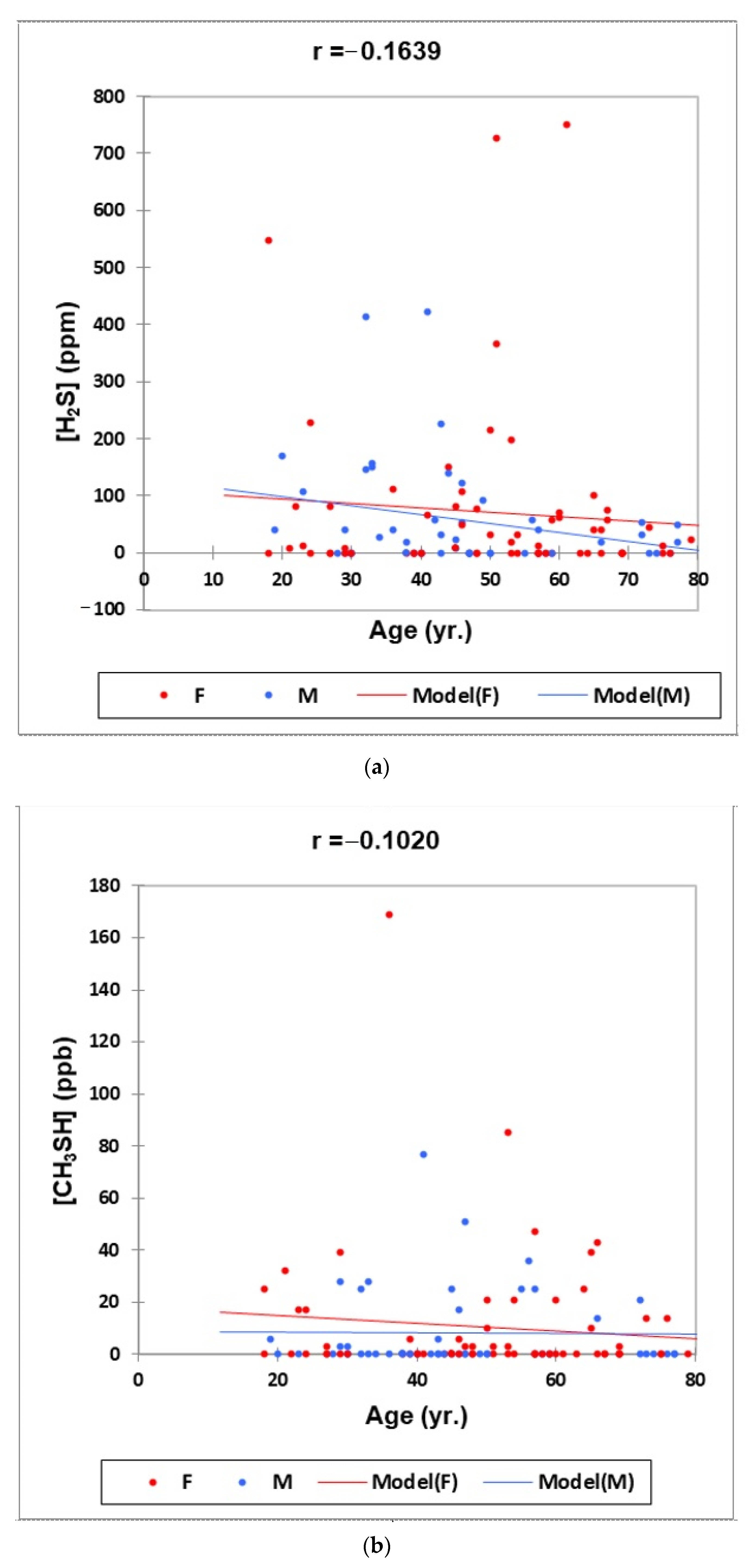
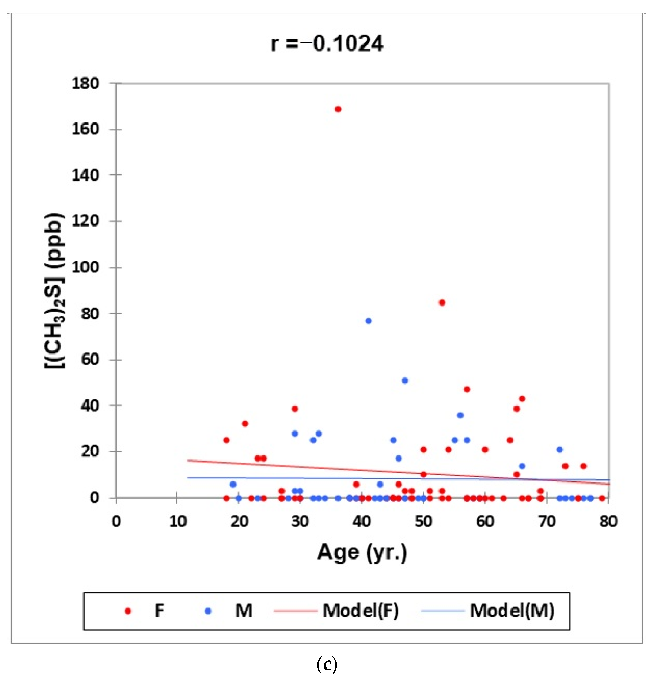
  • Figure 1: Plots of (a) H2S, (b) CH3SH and (c) (CH3)2S oral cavity air concentrations versus participant age for females (red) and males (blue) for the outlier-free dataset (n = 114). Correlation coefficient (r) values for these relationships are also provided.
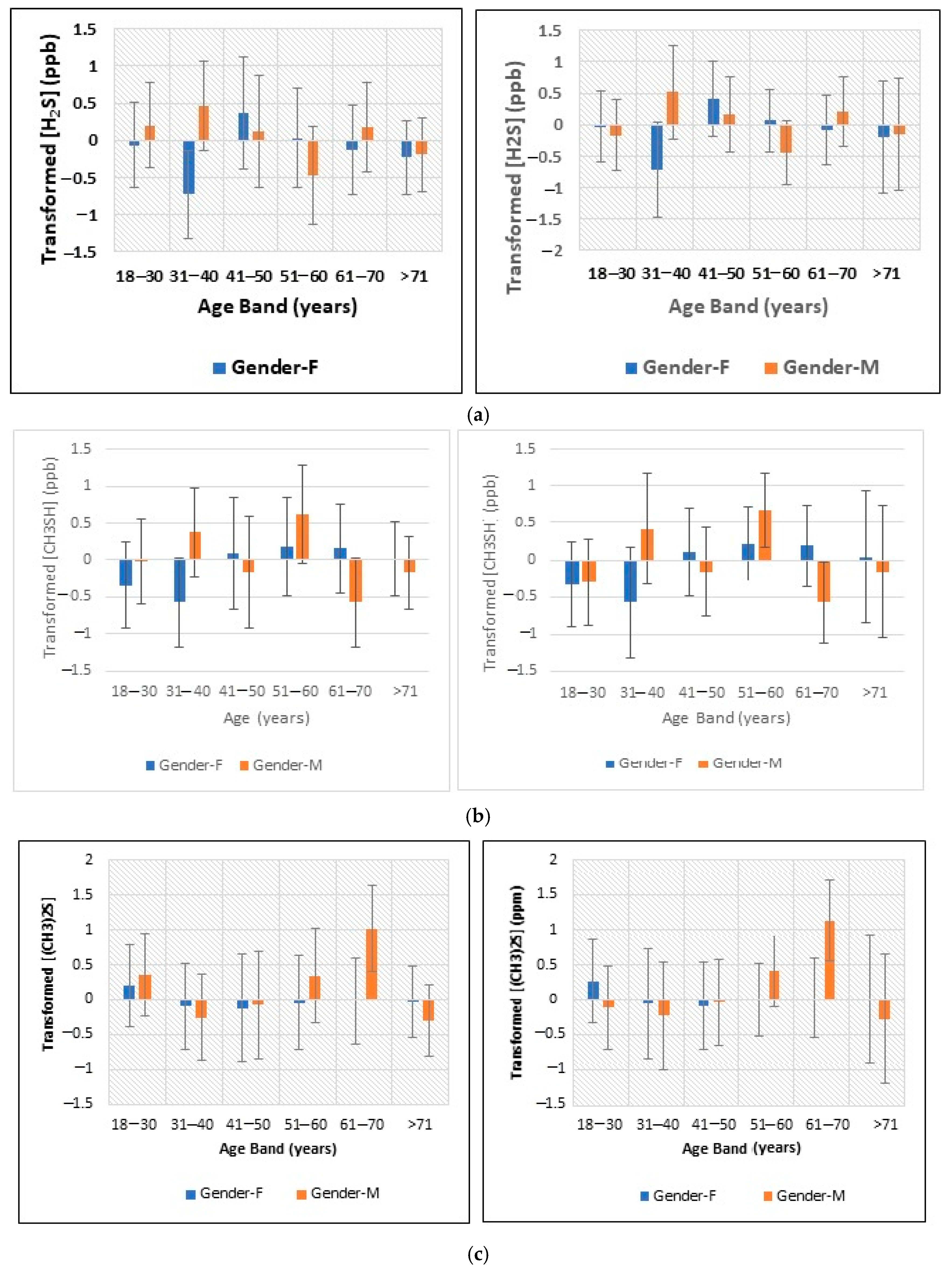
  • Figure 2: Plots of least squares mean ± 95% confidence intervals (CIs) for glog-transformed and autoscaled oral cavity concentrations of (a) H2S, (b) CH3SH and (c) (CH3)2S for each age band and gender featured in the analysis-of-variance-based experimental design applied (results obtained both before and after the removal of n = 2 possible outlier participant samples are shown).
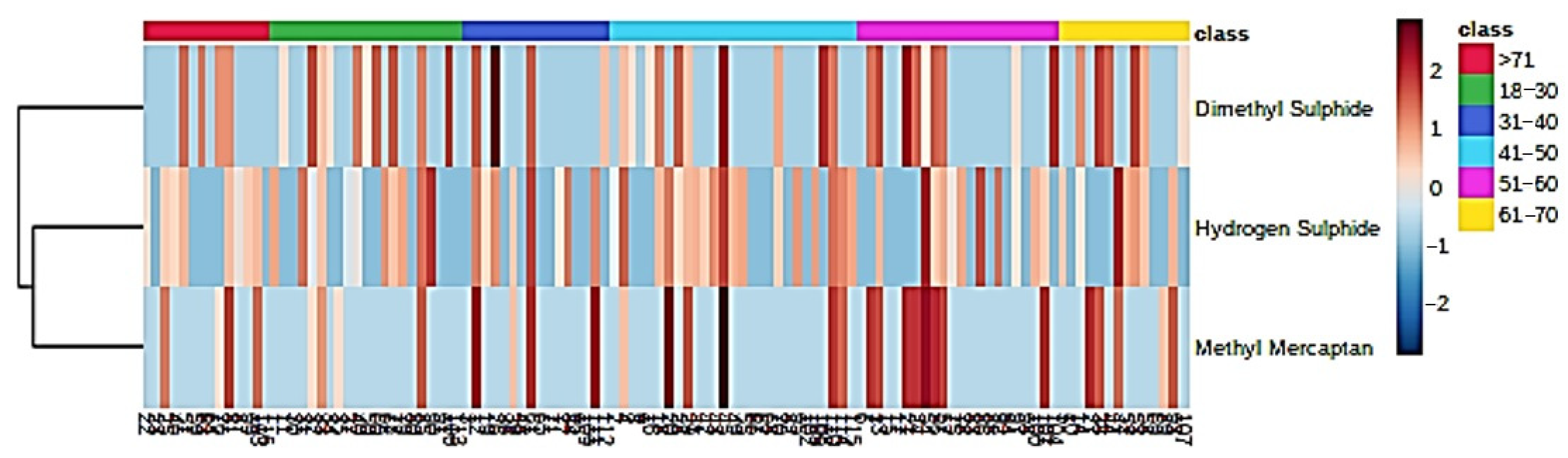
  • Figure 3: A monoclustering heatmap diagram based on Student’s t-tests displaying ‘between-participant’ variations in oral cavity VSC concentrations for each age band investigated (VSC levels were glog-transformed and autoscaled prior to analysis).
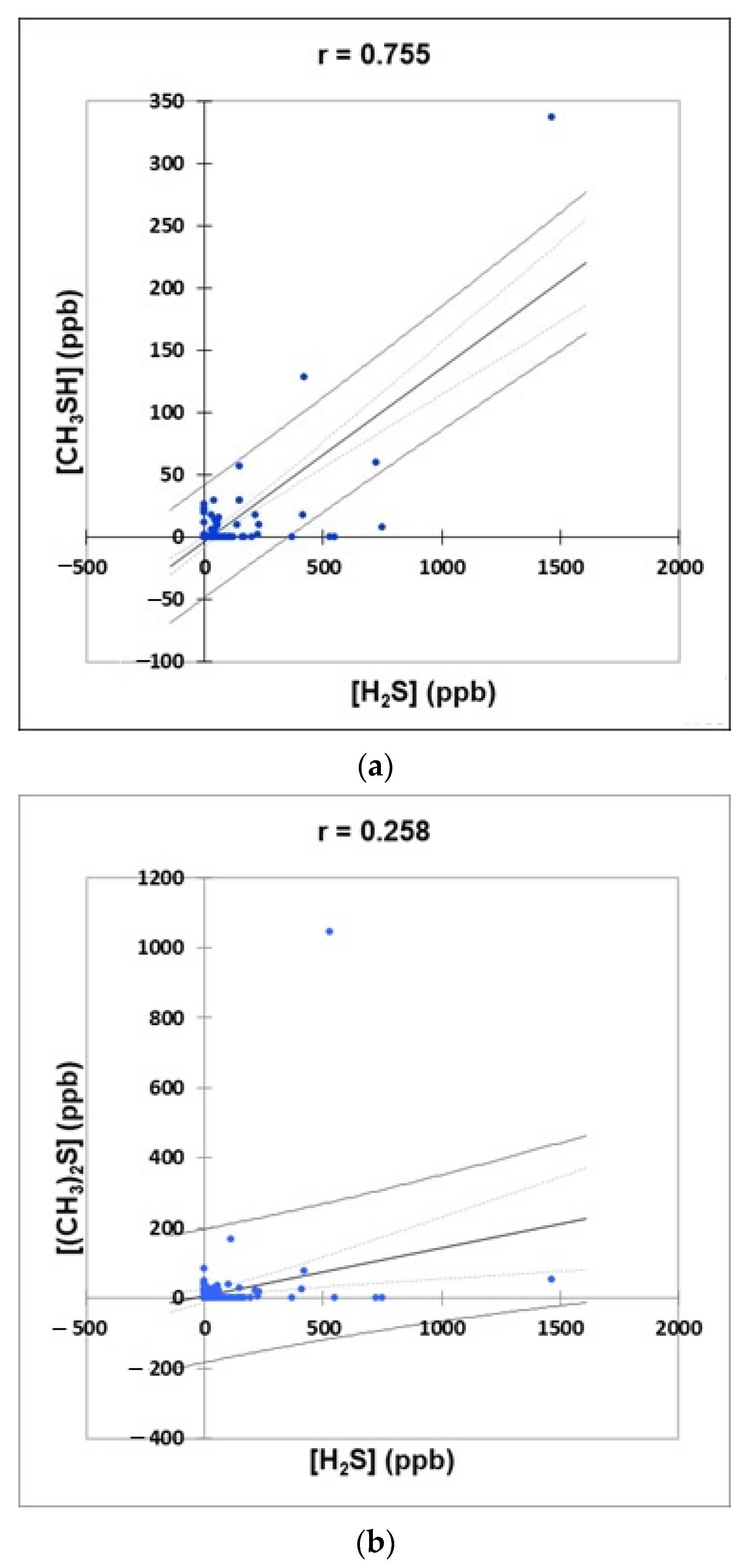
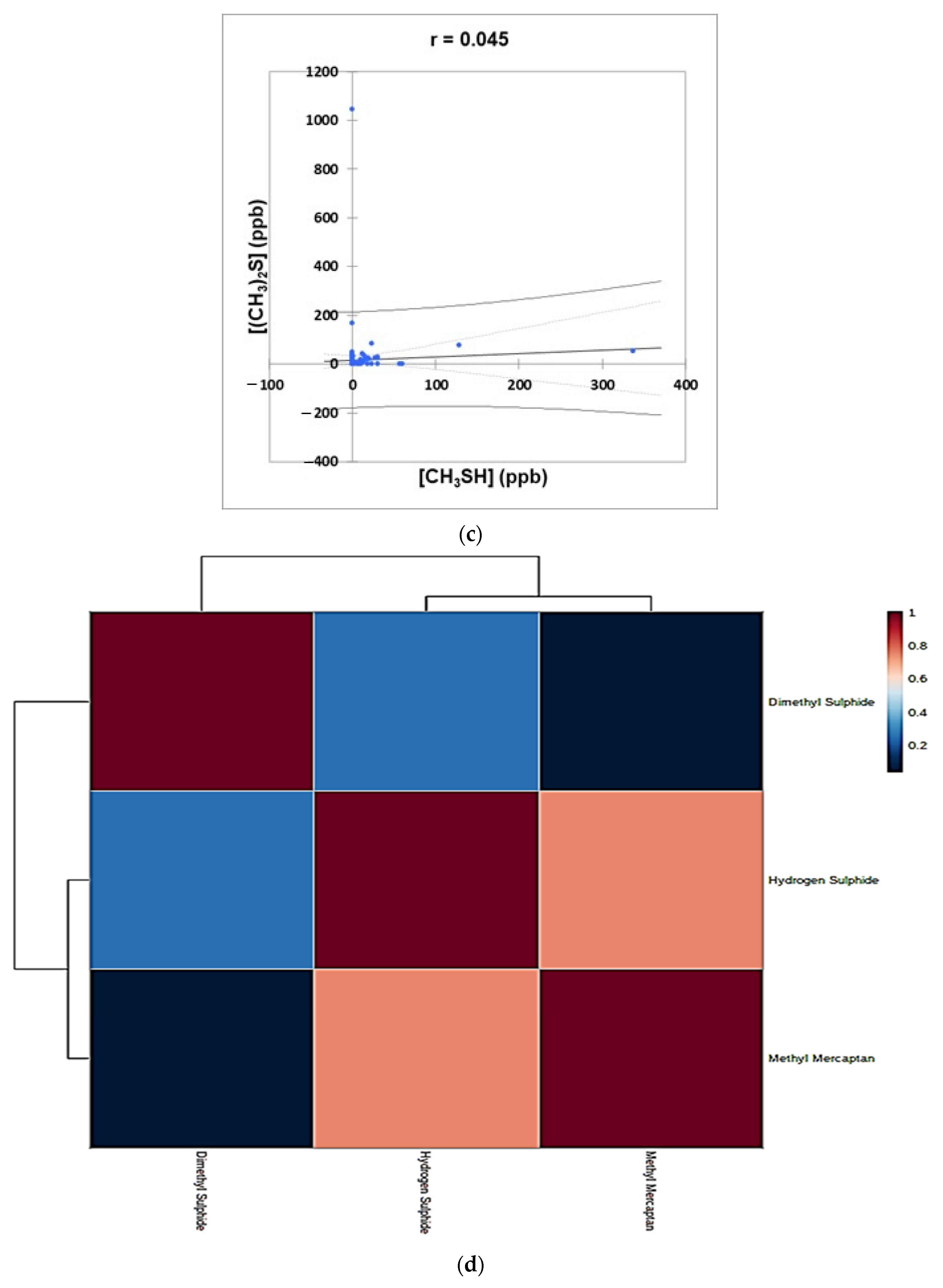
  • Figure 4: Plots of (a) CH3SH versus H2S, (b) (CH3)2S versus H2S, and (c) (CH3)2S versus CH3SH concentrations for the complete oral cavity VSC dataset. 95% confidence intervals (CIs) for mean values and observations are denoted. A clustering correlation heatmap is shown in (d).
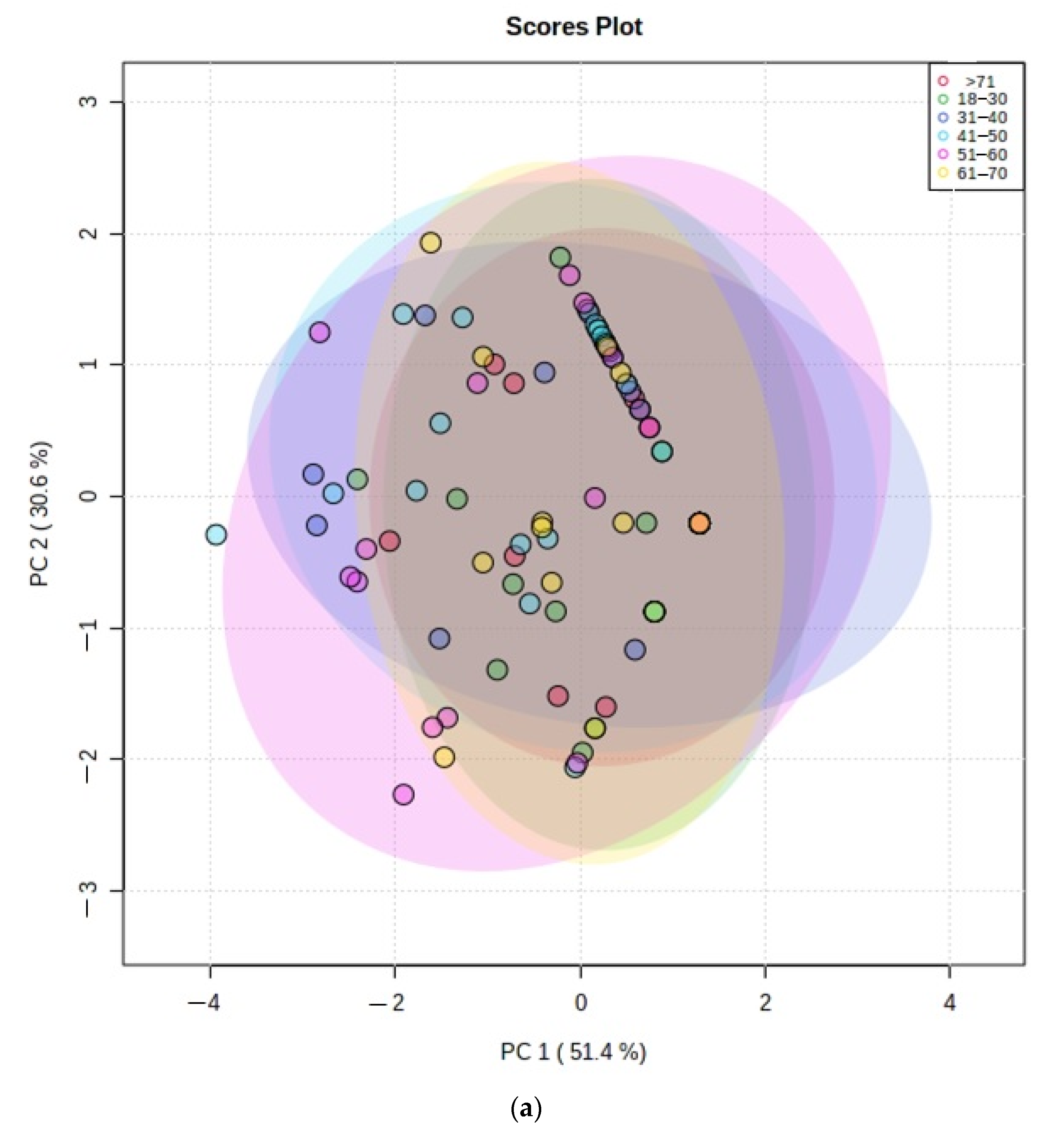
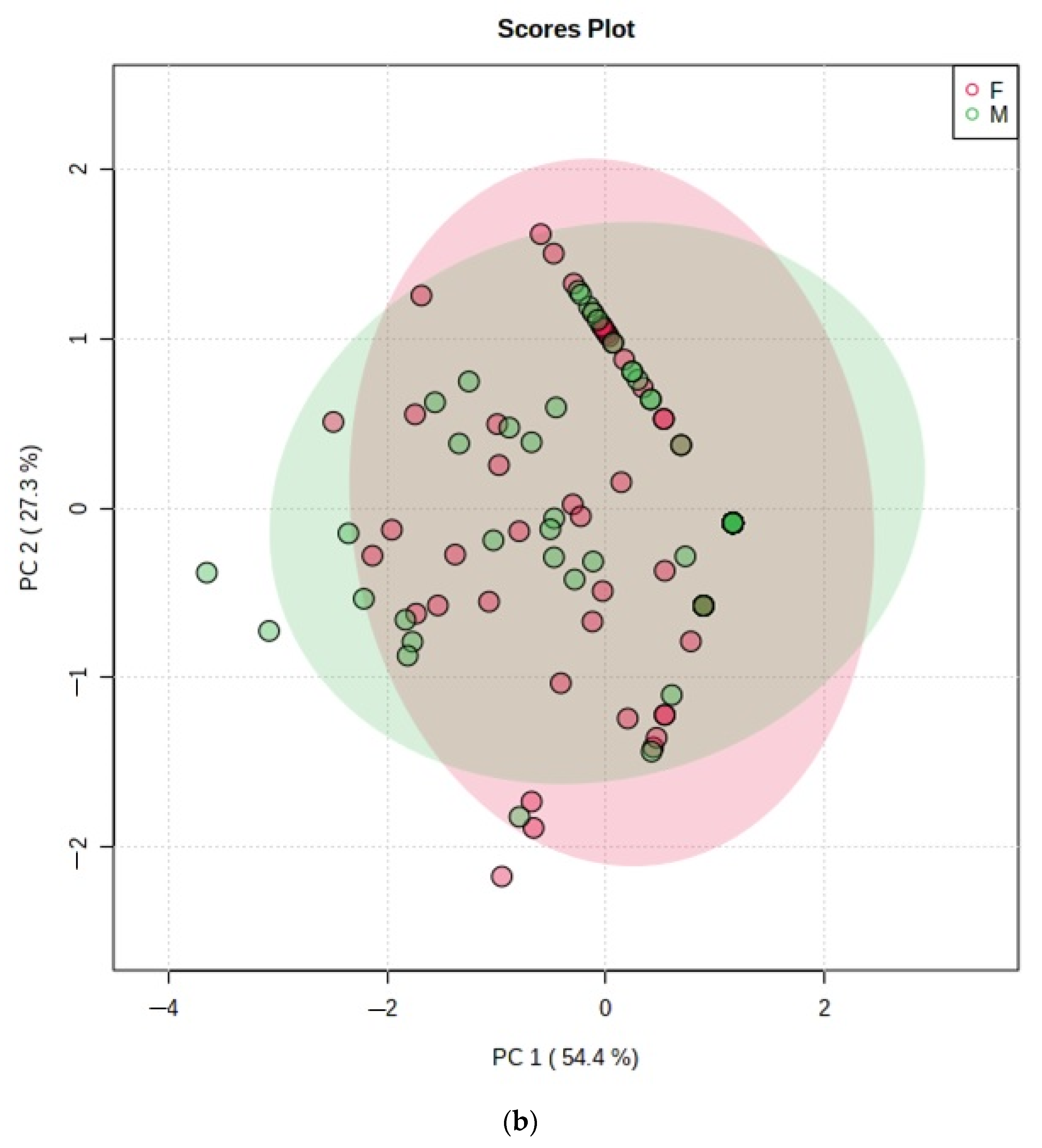
  • Figure 5: PCA scores plot with a maximum of two components demonstrating no distinctive clusterings between (a) age bands and (b) genders arising from the VSC dataset. Estimated variance contributions of PC1 and PC2 for PCA models are indicated,
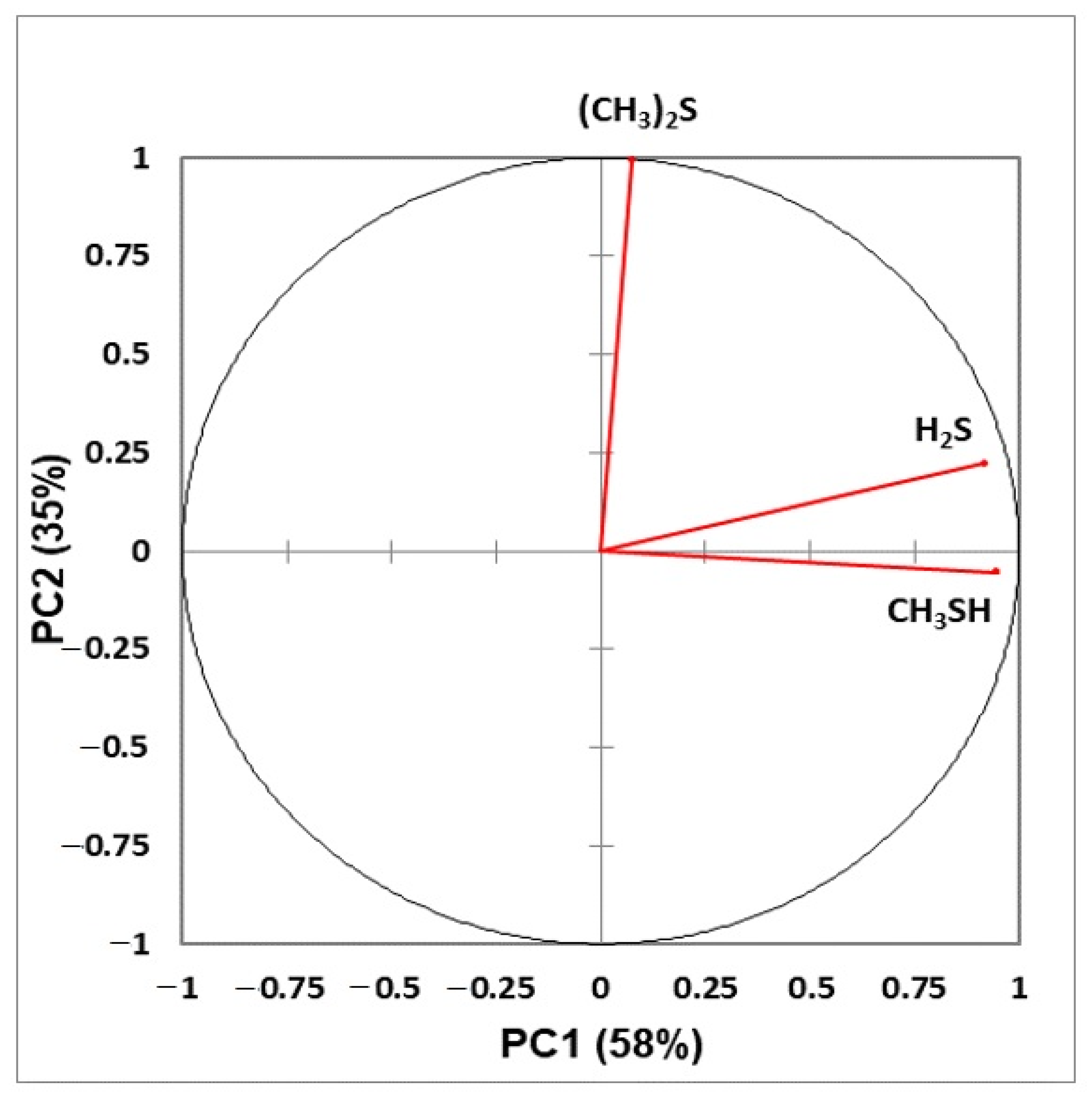
  • Figure 6: Correlation circle diagram displaying correlations between all explanatory variables considered, and principal components 1 and 2 in a principal component analysis model applied to the complete VSC dataset.
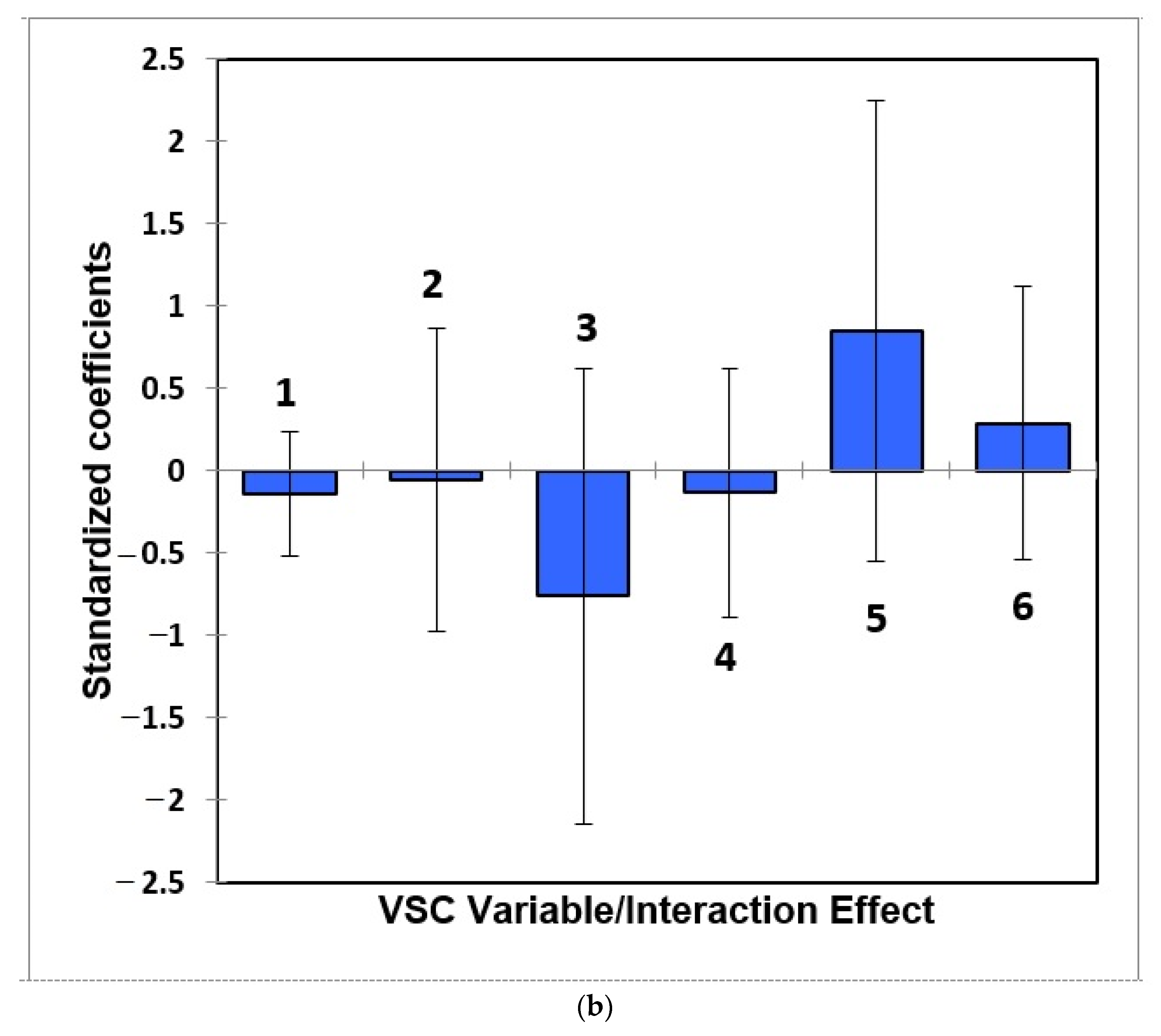
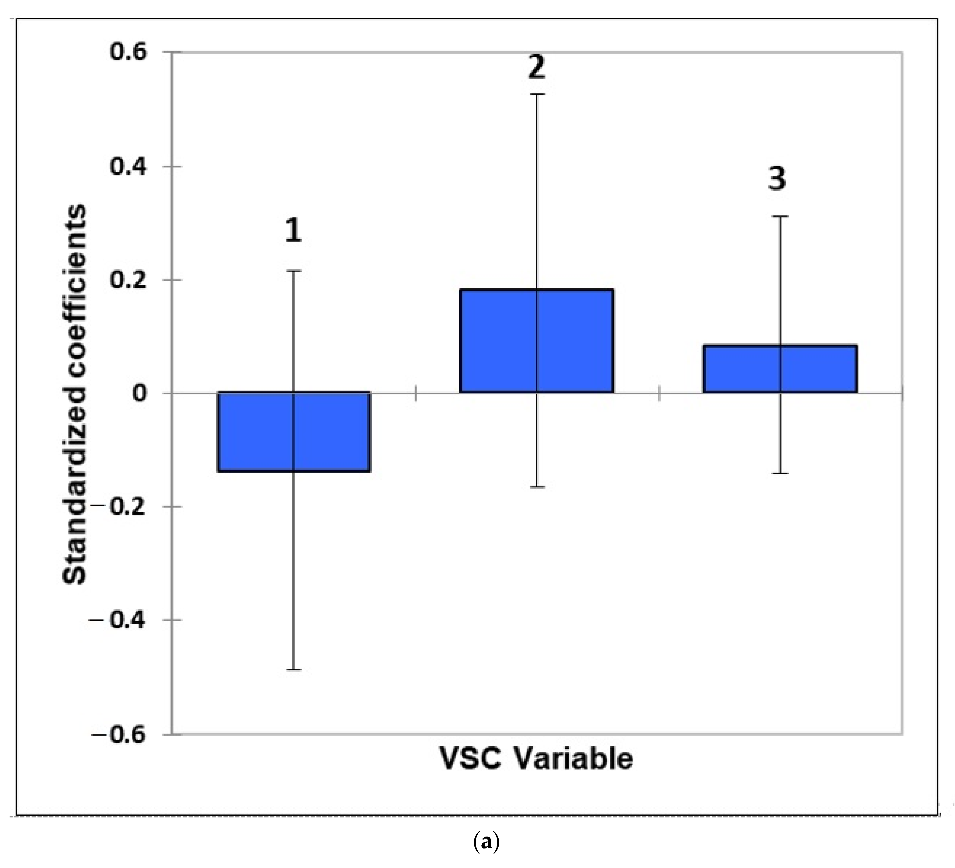
  • Figure 7: Estimated standardised coefficients ± 95% CIs for logistic regression analysis models constructed for prediction of the binary participant gender score variable (0 for females, +1 for males) from a model featuring (a) 3 VSC levels alone, and (b), as (a), but with their 3 first-order interaction effects also considered.
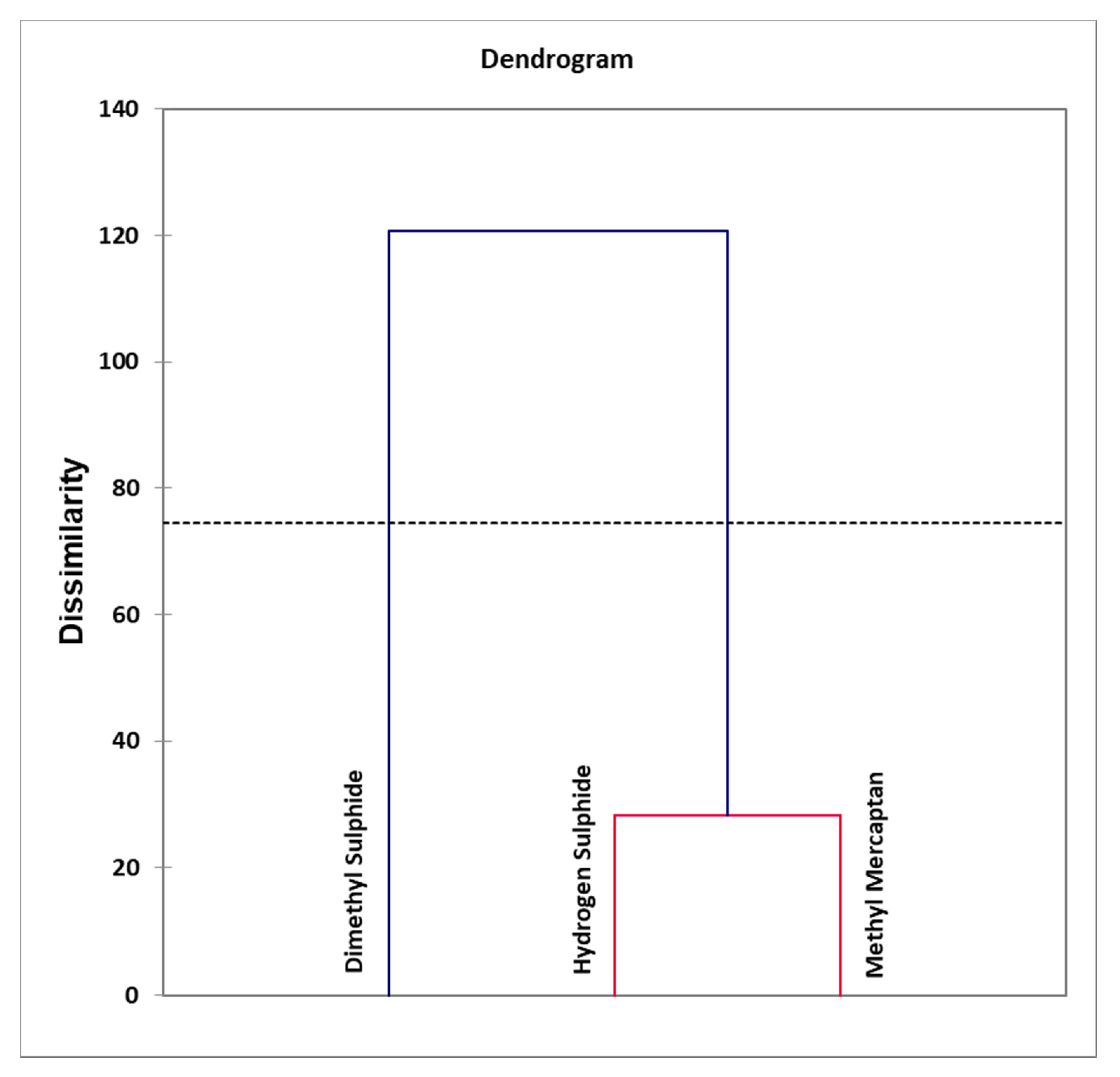
  • Figure 8: Agglomerative hierarchal clustering (AHC) dendogram diagram of VSC variables, revealing clear distinctions between clusters arising from an orally-sourced combination of correlated oral cavity H2S and CH3SH levels, and that of uncorrelated (orthogonal) extra-oral (CH3)2S. An automatic entropy-derived threshold limit is also shown.
  • Table 1: Frequency listing of numbers of study participants in each age band with oral cavity VSC levels greater than their threshold concentrations of malodorous objectionability (TCMO) limits.
  • Table 2: Pearson (n − 1) correlation matrix (correlation coefficient r values) for the raw oral cavity VSC concentration dataset (partial correlation coefficients are also provided). VSCs are indicated in the column and row headings.
  • Table 3: Principal component loadings vectors of VSC predictor variables (columns) following Varimax rotation and Kaiser normalisation featured in a principal component analysis (PCA) model of the complete dataset.
  • Appendix A: Brief Historical Review of the Development and Applications of Methods for Evaluating Oral Malodour in Humans
  • Appendix B: Short Outlines of the Principles and Applications of Multivariate (MV) Analysis Techniques Employed in Chemometrics and Metabolomics Investigations
  • Supplement: Complete VSC dataset with gaseous oral cavity H2S, CH3SH and (CH3)2S concentrations (ppb) listed in columns 4, 5 and 6 respectively. Corresponding samples codes, age bands and genders are provided in columns 1, 2 and 3 respectively.

2.1. Study Experimental Design and Criteria

This study involved 116 healthy non-smoking human participants (52 male/64 female) of age range 18–76 years. Samples were collected under conditions of informed consent according to the Declaration of Helsinki of 1975 (revised again in 2013). The positive response rate to advertisements for study participation was >70%; >65% (n = 116) of these advertisement respondents were deemed to be suitable for inclusion as participants. For primary screening purposes, all potential participants were required to complete a questionnaire which requested essential demographic information, medical and dental treatment history, and any current medications received. Exclusion criteria for this investigation are provided in the Methods section (Section 3). None of the recruited study participants had any prior knowledge of any pre-existing personal halitosis condition. VSC determinations (as parts-per-billion (ppb) oral cavity air concentrations) were performed on an OralChroma™ portable gas chromatographic (GC) monitoring system (details available in Section 3).
Oral cavity VSC measurements were made at 09.00–10.00 a.m. on sampling days, and all participants were required to agree to avoid their morning breakfast meal, and refrain from all further oral activities for a 4 h duration prior to sample collection. Participants were grouped according to the 18–30, 31–40, 41–50, 51–60, 61–70, and >71 year age bands, and also according to gender (full data file available in the supplement). H2S, CH3SH and (CH3)2S levels greater than their reported threshold concentrations of malodorous objectionability (TCMO) values of 95, 12 and 24 ppb, respectively [15], were detected in 22, 19 and 18 of the 116 recruited participants, respectively.

2.2. Statistical Analysis of Oral Cavity Volatile Sulphur Compound (VSC) Dataset

The experimental VSC dataset was analysed using a 2-factor analysis of variance (ANOVA), analysis of covariance (ANCOVA) and multivariate (MV) analysis of variance (MANOVA) models, partial and Pearson correlations, principal component analysis (PCA), partial least squares-discrimination analysis and -regression (PLS-DA and PLS-R, respectively), orthogonal partial least squares-discrimination analysis (OPLS-DA), ANOVA-simultaneous component analysis (ASCA), and an agglomerative hierarchical clustering (AHC) strategy. XLSTAT2014/2020 (Addinsoft, Paris, France) and MetaboAnalyst 5.0 (University of Alberta and National Research Council, National Institute for Nanotechnology (NINT), Edmonton, AB, Canada) software modules were employed for these analyses. The PLS-DA and -R approaches featured qualitative age band or gender, and quantitative age (years) and gender scores (0 for females, +1 for males) as response variables, respectively. The AHC model employed for clustering was constructed from dissimilarities between VSC variables based on Euclidean distance, Ward’s method of agglomeration; an automatic entropy truncation system was featured. Datasets were autoscaled but not glog-transformed prior to AHC analysis.
ANOVA and MANOVA models tested the statistical significance of the ‘between-age bands’ and ‘between-genders’ factors, together with the age × gender first-order interaction effect. For the MANOVA model, the significance of these sources of variation was determined using Wilks’ test (Rao’s approximation). Datasets for univariate (UV) analyses were generalized logarithmically (glog)-transformed and autoscaled in view of significant heteroscedasticities between age and gender test groups for all VSCs, and from the patterns of residuals arising from raw data ANOVA-predicted values (p < 0.05, Levene’s test). Autoscaling is a process which involves the mean-centering of column variables (VSC levels in this case), i.e., subtraction of the VSC column mean value from all observations in that column, followed by division by the column standard deviation; this gives rise to a set of 3 ‘standardised’ VSC variables which all have a mean value of zero and a variance of unity.
Ordinary least squares (OLS) multiple regression was performed using XLSTAT2020 software, with quantitative age or gender scores as the dependent response variables, and VSC concentrations, both with and without their first-order interaction effects, as independent ‘predictor’ variables. Equation (1) shows the mathematical model for this experimental design with all interaction effects considered, where H, M and D represent H2S, CH3SH and (CH3)2S levels, b0 the model y (ordinate axis) intercept, and b1 to b6 the partial regression coefficients for individual VSC variables (b1 to b3), and the VSC interaction effects (b4 to b6); eijk denotes fundamental error.
yijk = b0 + b1Hi + b2Mj + b3Dk + b4HMij + b5HDik + b6MDjk + eijk
χ2 contingency table analysis was conducted to investigate associations between the incidences of participants with one or more VSC level above the TCMO limits and age bands, and also genders, using an XLSTAT2020 software module. These were 3 × 7 and 3 × 2 contingency tables for investigating age bands and genders respectively. χ2 Fisher’s exact test was employed to determine statistical significance (threshold p value 0.050).
Two probable ‘outlier’ samples with oral cavity H2S, CH3SH and (CH3)2S concentrations of 1464, 337 and 54 ppm, and 529, 0 and 1044 ppm, respectively, were identified. Therefore, most of the statistical analysis strategies were applied to datasets both with and without the inclusion of these values.

2.3. Results

2.3.1. Exploration of Dependencies of Frequencies of Participants with VSC Levels above Their Threshold Concentrations of Malodorous Objectionability (TCMO) Limits on Age Bands and Gender: Contingency Table Analysis

Table 1 shows a listing of the numbers of study participants in each age group who presented with oral cavity concentrations of H2S, CH3SH and/or (CH3)2S in excess of the TCMO values specified above. A χ2 contingency test conformed that there was no significant association between age group and VSC nature regarding the numbers of participants scoring levels which were higher than the specified TCMO thresholds (p = 0.57). A corresponding contingency table analysis testing the non-independence of genders was also not significant (p = 0.50).
Of the n = 18 participants with (CH3)2S concentrations greater than the TCMO cut-off value, 12 of these values were higher than those of both H2S and CH3SH, and this may indicate non-oral sources for this VSC in these individuals. Moreover, for 5 of these participants, (CH3)2S was the only VSC detectable. A total of n = 30 participants had no VSCs detectable whatsoever; there was no significant association of the frequencies of these with age band (p = 0.75).
Preliminary plots of raw oral cavity VSC concentrations versus participant ages indicated very poor correlations between all VSCs determined and participant ages (Figure 1), none of which were found to be statistically significant (i.e., p > 0.05).

2.3.2. Preliminary Statistical Investigations: Correlations with Age and Gender

Mean ± standard error of the mean (SEM) H2S, CH3SH and (CH3)2S levels found in oral cavity air samples were 80.4 ± 17.4, 8.2 ± 3.2 and 18.8 ± 9.1 ppb respectively prior to removal of the 2 possible sets of outlier values, and 64.4 ± 12.1, 5.4 ± 1.5 and 9.5 ± 2.0 ppb thereafter. Hence, outlier removal diminished SEM values by about 30%, 53% and 78% respectively. Plots of VSC concentrations versus participant ages for both males and females in the outlier-audited dataset confirmed that there were no significant linear correlations between these variables for each VSC determined. Ranges for oral cavity H2S, CH3SH and (CH3)2S concentrations before outlier removal were 0–1464, 0–337 and 0–1044 ppm respectively, and 0–751, 0–128 and 0–169 ppm respectively, after.
Plots of H2S, CH3SH and (CH3)2S concentrations versus age (Figure 1) revealed no significant dependence of these VSC levels on this parameter both prior and subsequent to removal of the 2 outlier samples, even when males and females were considered separately.

2.3.3. Analysis of Variance (ANOVA), Analysis of Covariance (ANCOVA) and Multivariate Analysis of Variance (MANOVA) of the VSC Dataset

ANOVA analysis of the VSC dataset demonstrated that there were no significant dependencies of any oral cavity VSC levels on age bands, nor gender (p > 0.05, Figure 2), again for both outlier-containing and outlier-free datasets. Moreover, the first-order age × gender interaction effect was also not significant for all analytes. Similarly, performance of a corresponding ANCOVA model with the age variable as a quantitative explanatory variable, and incorporating the age × gender interaction effect, also found that none of the factors tested offered any significant contributions towards the variance of all 3 VSCs. Additionally, MANOVA analysis (described in Appendix B.1.1) of the full dataset confirmed that none of the above effects contributed significantly towards any of the oral cavity VSC concentrations (Wilks’ test p values ranging from 0.39 to 0.94).
A monoclustering heatmap diagram for the each of the different study age-bands is shown in Figure 3, with both up- and downregulated VSC levels indicated for all participants recruited to the study. Clearly, no ‘between-age band’ differences between VSC concentrations are visible in this diagram. However, application of the AHC technique to these data provided evidence for the division of the VSC potential predictor variables into two clusters, one consisting of a combination of H2S and CH3SH, the second with (CH3)2S alone. In view of this, this clustering of these VSC variables was further explored using a range of further MV and clustering analysis techniques (Section 2.3.5 and Section 2.3.7).

2.3.4. Correlations between Oral Cavity VSC Levels

Plots showing results from the regressions of CH3SH on H2S, (CH3)2S on H2S and (CH3)2S on CH3SH are shown in Figure 4a–c respectively. Clearly, there is a strong linear correlation between CH3SH and H2S (r = 0.755, p ≤ 10−21), but only a weak, albeit still statistically significant relationship between (CH3)2S and H2S (r = 0.258, p < 0.006); that between (CH3)2S and CH3SH concentrations (r = 0.045) was not significant. This is confirmed by the correlation heatmap shown (Figure 4d), which also shows two correlation-based clusterings containing (1) a composite of CH3SH and H2S, and (2) (CH3)2S alone. This again provides evidence for differential physiological site sources of these VSC clusters. A corresponding correlation matrix is displayed in Table 2. Both Pearson and partial correlation coefficients are listed therein.
Predictions of quantitative age and gender score ‘response’ variables using OLS regression analysis featuring all 3 VSC levels as potential predictor variables were all unsuccessful, with none of these variables proving to be statistically significant in both cases. Incorporation of the three first-order VSC interaction effects in the model failed to improve this.

2.3.5. Application of Multivariate Analysis Techniques: Principal Component Analysis (PCA), Partial Least Squares-Discrimination Analysis (PLS-DA), Partial Least Squares-Discrimination Regression (PLS-R), Orthogonal Partial Least Squares-Discrimination Analysis (OPLS-DA), Principal Component Regression (PCR) and ANOVA-Simultaneous Component Analysis (ASCA)

PCA and PLS-DA scores plots confirmed that there were no significant MV distinctions between any age bands, nor between gender classifications—PCA scores plots for the investigation of possible differences between different age bands and genders are shown in Figure 5a,b respectively. PLS-DA Q2 values of −0.04 and −0.35 were found for 2-component models considering age bands and genders as qualitative output factor classifications respectively (a value of +0.50 serves as a threshold cut-off value for an acceptable level of predictive classification success). Similarly, OPLS-DA also demonstrated that VSC concentration variables did not offer any ability to distinguish between participant age bands and genders. Likewise, both PLS-R and PCR analyses, with ages and gender scores as quantitative response variables, confirmed that none of the three VSC variables, nor the 2 components arising therefrom, served as significant features for predicting participant ages or gender scores.
A two-factor ASCA model, again considering the age band and gender factors, and their corresponding first-order interaction, as potential contributory sources of variation, similarly demonstrated that none of these effects were statistically significant; permutation testing p values obtained for these effects were 0.12, 0.57 and 0.70 respectively.
Notwithstanding this, PCA demonstrated that the 3 VSC variables were effectively segregated into two clear orthogonal components, the first containing a linear combination of H2S and CH3SH (loading vectors 0.92 and 0.95 respectively), the second (CH3)2S alone (loading vector 0.99), as shown in Figure 6 and Table 3. The PC loadings vectors of variables represent their degree of correlation with specific PCs; values of these which are lower or greater than the threshold values of −0.40 (for negative correlations with that PC) or +0.40 (for positive correlations with that PC), respectively, are generally accepted as ‘cut-off’ thresholds for significance.
Consistently, eigenvalues (i.e., the mean number of VSC variables loading on each PC) for PC1 and PC2 were 1.81 and 0.97 respectively, i.e., very close to their optimal values of 2.00 and 1.00, respectively, for a perfect model with two VSCs loading on PC1, and a single one loading exclusively on PC2. These results are fully compatible with the sources of these malodorous agents, i.e., H2S and CH3SH from the oral environment, and (CH3)2S from an extra-oral source. However, the very weak loading of the latter VSC on PC1 may indicate that a small proportion of it also arises from the oral environment.
These VSC variable component loadings were confirmed with the PLS-R and PCR analysis strategies applied, in addition to the PLS-DA approach. Indeed, the PLS-R and PLS-DA models developed exhibited strong loadings of H2S and CH3SH on component 1 (54.4% and 51.4% of total variance explained for datasets with and without outlier samples included, respectively), and (CH3)2S alone on PC2 (27.3% and 30.6% of total variance explained, respectively).

2.3.6. Logistic Regression Analysis Models

Subsequently, logistic regression analysis (logRA) was applied as an alternative protocol in an attempt to predict age bands and gender scores of participants. Models were developed both with and without the consideration of VSC interaction effects, and also the use of a PCR-logistic regression variant (logPCR) for the binary gender score variable. However, all forms of logRA were completely ineffective in predicting the multinomial gender age band variable, and both this and the logPCR approach were unsuccessful in distinguishing the binary gender score variable. Indeed, overall classification success rates were only 26.4% and 27.4% for the logRA technique applied to age bands without and with the inclusion of first-order VSC interaction effects, respectively, Moreover, corresponding success rates for binary gender score classification were only 48.3% and 50.0%. Bar diagrams of standardized coefficients for VSCs and their corresponding 95% CIs for gender score prediction models, with and without the incorporation of second-order interaction effects, are shown in Figure 7. Clearly, none of the VSC variables were found to contribute towards gender score variances significantly.

2.3.7. Agglomerative Hierarchal Clustering (AHC) Analysis Model Conducted with Truncation Threshold Limit Setting

Finally, an additional AHC analysis model performed with the computation of an automatic entropy truncation threshold limit confirmed resolution of the VSC predictor variables into two highly-significant clusterings: (1) an H2S/CH3SH composite, and (2) (CH3)2S exclusively (Figure 8). Indeed, the dotted horizontal truncation limit displayed in this figure indicates a clear dissimilarity between these two clusters, but not between H2S and CH3SH. As expected, AHC analysis of the samples themselves failed to facilitate the clustering of the oral cavity air samples collected into differential participant age band, nor gender, classifications.
A repeat of this AHC analysis conducted following removal of the n = 2 possible outlier samples gave rise to exactly the same independent H2S/CH3SH combination and (CH3)2S only clustering results (data not shown).

2.4. Discussion of Results Obtained

Results acquired in this study provided evidence that for a large group of healthy, or perceivably healthy human participants, there was no statistically significant dependence of oral cavity VSC concentrations on the demographic variables ages and gender. Moreover, there was also no age band- or gender-related differences between the frequencies of these healthy participants with oral cavity H2S, CH3SH and (CH3)2S levels above their specified TCMO limits (approximately 20% for each one). From the OralChroma™ manufacturer, a significant oral malodour condition exists when the oral cavity concentrations of H2S or CH3SH exceed 112 and 26 ppb respectively, the former being very similar to that specified in [15], although the latter is 2-fold higher. Nevertheless, the possibility that perhaps some the about 15% of healthy participants with (CH3)2S levels above the TCMO limit having unknown or unspecified extra-oral conditions giving rise to these high concentrations cannot be ruled out. Notably, in a related baseline study, Snel et al. [20] found that the median oral cavity (CH3)2S level in the morning awakening breath of a group of healthy subjects was 20 ppb (range 0–217 ppb), a value very similar to its TCMO value of 24 ppm.
Further support for the lack of age- or gender-dependencies of oral cavity VSC contents was provided by each of the data analysis strategies applied, which were of a highly rigorous nature, and which included the tracking of sample outliers. Factorial ANOVA coupled with the MV analysis techniques PCA, PLS-DA and OPLS-DA confirmed that all VSC concentrations determined were independent of both age band and gender. Indeed, all these MV statistical techniques applied, along with AHC analysis, clearly demonstrated that the VSC predictor variables were partitioned into two clear orthogonal components, the first containing orally-generated and strongly correlated H2S and CH3SH levels, the second only extra-orally-formed (CH3)2S concentration, which was found to be much less correlated or uncorrelated with those of H2S and CH3SH. These VSC variable component loadings were confirmed using the PLS-R, PCR and logPCR strategies applied, with age and gender score used as quantitative response variables.
Such a conclusion would not be readily derivable from the application of UV statistical analysis techniques alone such as OLS and logRA since these methods are unable to cater for variable multicollinearities. Hence, it appears that MV methods of statistical evaluation rather than ordinary least squares (OLS) and logRA multiple regression techniques are best suited to the analysis of relatively simple VSC models featuring only 3 ‘predictor’ variables. In addition to the powerful positive correlation of H2S and CH3SH concentrations observed here, multicollinearity variance inflation factor (VIF) statistics for VSC variables in OLS models constructed, which varied from 1.14–2.63 for the n = 116 raw VSC dataset, and 1.14–1.30 for the n = 114 glog-transformed and autoscaled one without 2 likely outlier samples, were considered to be statistically significant (VIF values of 1–5 usually indicate moderate, albeit significant correlations) [21]. This again fully justifies the use of more complex MV analysis approaches for analysis of the VSC dataset acquired here.
However, since it is certainly conceivable that not all (CH3)2S arises from a non-oral, blood-borne source, the marginal correlation of H2S level with it found here (r = 0.258, and 0.342 for its corresponding partial correlation coefficient), which was also highly statistically significant (p < 0.006), may indicate this.
The oral generation of malodorous VSCs and other bacterial catabolites is commonly linked to microbial infiltration on or within the tongue dorsum. dental and mucosal surfaces, and periodontal pockets, predominantly that of gram-negative proteolytic bacteria. Notably, the major source of such microbial-derived metabolic by-products is residual food fragments which adhere to oral surfaces. However, the fermentation of proteins available in oral fluids, and in lysed and desquamated cells, represents a less frequent source [22].
In 2011, Porter et al. [23] reviewed the influence and reciprocity of diet and gastrointestinal (GI) tract disease on oral malodour. Although the consumption of selected odiferous foods such as garlic or onions, etc., gives rise to a transiently-modified, often adverse breath odour, established halitosis conditions predominantly result from relatively common oral diseases, e.g., gingivitis or periodontitis. Notwithstanding, there is now some evidence available that oral malodour may also arise from diseases of the upper GI tract, and that future therapeutic strategies for halitosis may be facilitated by the influence of selected dietary agents which have the ability to inhibit the production of VSCs by bacterial enzymes.
Snel et al. [20] also reported the morning breath VSC contents of a group of healthy control participants, and for this purpose their study involved the collection of 3 samples per individual at different time-points following morning wake-up, specifically immediately after waking, and then before and after a breakfast meal; all 3 samples were collected within an estimated 1 h period. Samples collected immediately following waking (morning breath) were found to contain the highest VSC levels, followed by significant reductions thereafter. However, no significant differences in VSC levels between the pre- and post-breakfast samples were found.
Hence, on considering study timelines, it would appear that the pre-breakfast samples collected during the reference investigation reported in [20] probably best approximates those collected in the current study, and mean levels determined in these were about 50, 40 and 20 ppb for H2S, CH3SH and (CH3)2S, respectively. These values certainly do not differ significantly from those found in the current study, in datasets both with and without outlier sample inclusion. Ref. [20] also found that H2S levels were very significantly correlated with those of CH3SH (r = 0.65), but not between (CH3)2S concentration and either H2S or CH3SH. Hence, these results are entirely consistent with those found in our study (corresponding r value 0.755, Table 2).
Again, Snel et al. [20] found no significant correlations of any VSC level with participant ages, as observed here. However, statistically significant increases in H2S and CH3SH concentrations, albeit with p values only <0.05, were found in female participants over those of males, but not so for (CH3)2S. However, this effect may be limited to early morning breath samples only. Nevertheless, the influence of gender on oral cavity VSC concentrations remain somewhat controversial. Indeed, in a very large group of 2672 daily-sampled Japanese adults, no significant gender-mediated differences in VSC levels were found in a wide series of age groups tested [2].
From reference [20], it was also concluded that early morning breath should be recognised as a surrogate objective for therapeutic interventions focused on improvements in breath quality. Moreover, these researchers also found a considerable day-to-day variation in VSC levels that were not associated with dietary (breakfast) intake.

2.5. Conclusions

In conclusion, no evidence for the dependencies of oral cavity VSC concentrations on participant donor ages, nor genders, was obtained for a healthy cohort of human participants. MV data analysis provided evidence that oral cavity VSCs may indeed arise from different localizations, the first intra-oral sources, i.e., from Gram-negative bacterial preponderance at tongue dorsal. dental and mucosal surfaces, and/or within periodontal pockets (a combination of H2S and CH3SH), the second an extra-oral, presumably blood-borne one ((CH3)2S alone). Such data analysis techniques are, therefore, recommended for future investigations of halitosis and its VSC origins in a range of human diseases, both oral and extra-oral. Intriguingly, excessive oral cavity air (CH3)2S levels may serve as valuable indicators of extra-oral disease pathogeneses.

2.6. Potential Limitations and Strengths of the Study

One limitation of this study is the absence of a full clinical assessment to evaluate the oral health status of participants, although potential participants were excluded from the study if they indicated that they have had any current or recurring serious oral health/dental condition, or if they had undergone any treatment for one within 6 months of the pre-specified study sampling day. Moreover, it should also be acknowledged that self-reporting participant bias may also have exerted a significant impact on our research findings. However, the exclusion criteria listed were very rigorous (Section 3.1).
Another complication is that the resting salivary flow-rate of participants was not determined in this study; this parameter, along with probing pocket depths of ≥5 mm, bleeding on pocket probing, and elevated tongue coating scores are also considered to represent powerful contributory criteria which influence oral malodor findings [24].
One additional consideration is that only a single set of 3 VSC determinations was made per participant in view of study time constraints. Notwithstanding, if two consecutive determinations were made per participant, unfortunately they would not represent exactly matching duplicates since an 8 min. period was required for complete VSC analysis, and hence the second ‘replicate’ oral cavity air sample for analysis would not be collected until about 10 min. later.
A further limitation is that this study was restricted to healthy or perceivably healthy control participants only without any potentially confounding serious chronic medical or oral health conditions. However, a major expansion of this halitosis study to participants with a wide variety of clinical conditions is planned for the near future. This future study, with a meticulously planned protocol and experimental design, will conceivably provide valuable information regarding relationships between the presence and/or severity of such conditions (e.g., non-communicable chronic diseases such as cancer, cardiovascular disorders and diabetes) and patterns of oral cavity VSC levels, which may be extended to an evaluation of halitosis incidence and VSC sources in such patients.
The strengths of this study largely arise from the relatively large sample size (>100 participants) and the very favourable response rate of requested participation. Indeed, this permitted and facilitated the application of a series of MV statistical analysis techniques, which assisted with the control of potentially confounding factors. Moreover, this large sample size facilitates extrapolation of the results acquired to populations with similar demographic attributes.

3. Methods

3.1. Exclusion Criteria

Participants were excluded from the study if they were pregnant; were aged <18 years; had any serious or chronic medical condition such as diabetes, cardiovascular diseases or cancer, etc.; were tobacco smokers; had any recorded respiratory tract infections 2 years prior to the sampling test day; had any systemic disease associated with oral malodour, including renal illness, gastrointestinal disorders and cirrhosis, etc.; had a record of dental decay; had any periodontal or dental caries treatment within the previous 6 months; had an absolute minimum of 12 teeth; had any form of removable or fixed dental prostheses; were not under any medication which may interfere with VSC generation for the previous 6 months, e.g., antibiotics, antidepressants and/or antihistamines. Participants were also excluded from the investigation if they had received any form of medication during the 7 days prior to or on their VSC testing day. There was no upper age limit for study participation.
On their VSC assessment testing day, eligible participants were requested to forgo their early morning breakfast meal, and all further oral activities 4 h prior to sample collection, including their usual oral hygiene practices (including the use of toothpastes, oral rinses and breath fresheners), chewing gum and tobacco smoking. Participants were also requested to avoid eating odorous foods and drinking alcoholic beverages within a 48 h period prior to their assessment day.

3.2. Details of VSC Measurements

Oral cavity VSC measurements were made at 09.00–10.00 am on all sampling days involved (n = 116 participants). VSC determinations were conducted on an OralChroma™ portable GC monitoring system. Participants were requested to sit back on an appropriate stable chair. Primarily, a sterile plastic 1.00 mL volume syringe was inserted deep into their oral cavities, which was then retained there for a duration of 3.0 min. whilst participants closed their mouths tightly. Subsequently, the plunger was slowly pulled, pushed in again and then pulled to a 1.0 mL volume prior to removal from the mouth (care was taken to avoid allowing the syringe to come into contact with the tongue or saliva). A dedicated VSC analysis needle was then attached to the syringe unit. Sampled 1.0 mL volumes of oral cavity air were then reduced to exactly 0.50 mL via ejection, and these aliquots were injected into an OralChroma™ device (duration between sampling and GC analysis injection loading ≤5 s). The analysis was then commenced automatically. Participants refrained from talking for 5 min. prior to measurement, and also consented to breathe through their noses during the collection of oral cavity air samples via syringe insertion. Results were recorded as ppb oral cavity H2S, CH3SH and (CH3)2S concentrations (Table S1).
Although the specificity of VSC determinations made using this instrument may be potentially influenced by interfering levels of oral cavity acetaldehyde and isoprene [25], previous investigations have noted that they do not affect VSC analysis results significantly in view of their relatively very low concentrations in this environment [15,26]. The sensitivity of VSC determinations made by the OralChroma™ instrument is reported as about 3 ppb [17].

Supplementary Materials

The following are available online at https://0-www-mdpi-com.brum.beds.ac.uk/article/10.3390/data6040036/s1, Table S1: Complete VSC dataset with gaseous oral cavity H2S, CH3SH and (CH3)2S concentrations (ppb).

Author Contributions

Conceptualization, M.G. and K.L.G.; methodology, M.G., V.R.-R. and K.L.G.; software, M.G.; validation, K.L.G. and M.G.; formal analysis, M.G. and V.R.-R.; investigation, K.L.G., V.R.-R., and M.G.; resources, M.G.; data curation, K.L.G. and M.G.; writing—original draft preparation, M.G.; writing—review and editing, M.G. and K.L.G.; visualization, K.L.G.; supervision, M.G.; project administration, M.G.; funding acquisition, Not applicable. All authors have read and agreed to the published version of the manuscript.

Funding

This research received no external funding.

Institutional Review Board Statement

The study was conducted according to the guidelines of the Declaration of Helsinki, and approved by the Institutional Review Board (or Ethics Committee) of the Faculty of Health and Life Sciences, De Montfort University (protocol code 1117, date of approval 1 August 2015).

Informed Consent Statement

Informed consent was obtained from all subjects involved in the study.

Data Availability Statement

Data supporting reported results can be found in the Supplement provided.

Acknowledgments

The authors are very grateful to all the participants who took part in this study.

Conflicts of Interest

The authors declare no conflict of interest.

Appendix A

Brief Historical Review of the Development and Applications of Methods for Evaluating Oral Malodour in Humans

Determinations of the precise molecular nature and magnitude of oral malodour principally require reliable, sensitive, accurate and precise experimental and instrumental techniques, and previously reported strategies available for the monitoring of VSCs include organoleptic (subjective) methods [27,28], their direct determination by conventional gas chromatography (GC) combined with flame-photometric detection systems [29], a composite of the above two approaches [30], cryo-osmoscopy [31], or the time-consuming, onerous culture of periodontal pocket and plaque exudates in selected bacteriological culture media [13]. Notwithstanding this, to date there are only a limited amount of experimental data available on the applications, reliabilities and reproducibilities of such bioanalytical strategies, and there are sometimes many complications experienced with the exclusion of potentially interfering participant factors, such as the menstrual cycle, variations in oral hygiene control, circadian variation, smoking habits, and climate in general [32]. Furthermore, subsequent to evacuation of malodorous gases from the oral cavity, their restoration rate and extent to this environment remain debatable.
However, in the early 1990s a portable industrial H2S/CH3SH-specific VSC monitor (halimeter) became available, and early reports outlining its successful application in clinical practice are available in [33,34]. Indeed, highly significant correlations between these measurements and those achieved via synchronous organoleptic assessments completed by a series of rating judges have been reported [33]. The electrochemical VSC monitor involved consisted of a voltammetric sensor which drew a sample of oral cavity air across an electrocatalytic sensing electrode operating at a potential of +0.50 V; this operating potential is sufficient to ensure effective and reliable responses from the oxidation of electron-donating VSC thiol equivalents, i.e., those of CH3SH and H2S; redox potentials (Eo) of thiol/disulphide couples generally lie within the −0.20 to +0.40 V range. These electrochemical processes give rise to an electric current, the magnitude of which is directly proportional to total chemically-reducing, oral cavity air VSC levels. This current is transformed to a voltage, which, is subsequently transferred to a meter which provides gaseous VSC levels in parts-per-billion (ppb) over a 0–1000 ppb calibration range. Notably, oral cavity VSC measurements made with this device have been shown to be more precise and reproducible than those obtained by subjective, organoleptic panel methods. Moreover, there is evidence that they exhibit a greater sensitivity to diminutions in VSC concentrations induced by oral healthcare product treatments [33,35]. However, as noted above, a disadvantage of this device was that it was only able to monitor the combined reducing activity of only two VSCs, namely H2S and CH3SH, and not that of (CH3)2S. Another early example of the rigorous employment of this device can be found in the study described in [36], in which it was employed to monitor the ability of a series of oral health formulations to suppress oral cavity VSC (combined H2S and CH3SH) concentrations in a group of n = 6 participants, who underwent no fewer than 7 treatment regimens; halimeter response measurements were made at 5 diurnal time-points.
Advantageously, since 2011, a more specific, non-stationary gas chromatographic VSC determination instrument has been made available (OralChroma™, Nissha Co., Ltd., Nakagyo-ku, Kyoto 604–8551, Japan), reviewed in [37]). This device offers many advantages over the above halimeter facility, and has the ability to specifically determine ppb oral cavity ppb concentrations of H2S, CH3SH and CH3SCH3 concomitantly in a measured volume of air directly sampled from the oral cavity via a disposable plastic syringe; each level is displayed on a convenient display panel. An example of its use, which demonstrates its ability to determine the longevity of the VSC-neutralising actions of an oral rinse product, is available in [38]. Of course, this VSC monitor offers many bioanalytical benefits over more complex, traditional GC-based methods, the routine use of which are prohibitively restricted at most ‘point-of-care’ clinical sites, such as dental surgeries, health centres or pharmacies, in view of their preclusively large sizes, costs, and requirement for specialist, dedicated technical staff for their management and operation. Hence, further advantages offered by this readily portable VSC determination instrument include markedly lower costings than those required for the purchase, sample processing and operation of more conventional large GC facilities, rapid sample throughput, facile ‘on-site’ use in clinical settings, no demands for specialist support technical staff, and the ease of oral cavity air sample collection for analysis. In view of these benefits, this OralChroma™ facility was employed for the purpose of oral cavity VSC determinations in this study.

Appendix B

Appendix B.1. Short Outlines of the Principles and Applications of Multivariate (MV) Analysis Techniques

Employed in Chemometrics and Metabolomics Investigations.
For the benefit of readers who are unfamiliar with MV statistical analysis techniques frequently employed in ‘state-of-the-art’ metabolomics and chemometrics investigations, an outline of some of the more commonly used approaches are provided below in Appendix B.1.1Appendix B.1.6, Readers are referred to refs. [39,40] for further information.

Appendix B.1.1. Multivariate Analysis-of-Variance (MANOVA)

MANOVA represents a generalisation of ANOVA which extends to the study of several outcome variables simultaneously, and is generally applicable to datasets which have several inter-related outcome variables which cannot be satisfactorily addressed by consideration of only a single variable. In such cases where the outcome variables are correlated, analysis of these independently as single variable systems usually provides models which are highly unsatisfactory, and therefore an alternative analysis, which considers all response variables simultaneously, is required. Hence, when applied to such systems, MANOVA serves to explore MV outcomes observed for all explanatory variables considered, for example age band/age, gender/gender score and their first-order interaction effects as possible contributors to 3 molecularly-distinct VSC levels as in this study. If any of the above 3 omnibus MV evaluations (specifically, the main factor effects of gender score/gender and age band/age, together with the gender band/gender x age band/age interaction sources of variation) are statistically significant, subsequent post-hoc tests may be performed to determine the sources of group differences (Wilks’ test employed here is one example).

Appendix B.1.2. Principal Component Analysis (PCA)

PCA is an unsupervised MV analysis process which involves the computation of a relatively small number of principal components (PCs) from datasets usually containing large numbers of possible individual ‘predictor’ variables. Each PC consists a linear combination of a series of such predictors which are correlated with each other, either positively or negatively, and either strongly or moderately so. The first, most prominent PC (PC1) accounts for the greatest amount of dataset variation, and this is then followed by the second PC (PC2), which contains a second set of correlated variables and is orthogonal to (i.e., completely uncorrelated with) PC1, and which accounts for the second largest amount of dataset variation, Likewise for the third, fourth and fifth PCs (PC3, PC4 and PC5 resepctively), along to the nth PC value. Hence, PCA is a technique that can condense medium, large or very large-sized datasets, sometimes with several thousand possible predictor variables, to a much smaller number of uncorrelated PCs, each one containing a combination of n correlated, possible predictor molecules. Hence, this strategy, and also that of factor analysis, has the ability to determine differential sources of or explanations for orthogonal PCs. Variables such as biomolecule concentrations which load strongly on the same PC often provide similar or related information, diagnostic or otherwise, since they are correlated with each other and, therefore, they may arise from the same source, for example the same metabolic pathway in metabolomics investigations. Hence, PCA is used to effectively alter the basis of complex large predictor variable datasets, frequently by employing only the first 2, 3 or 4 PCs and disregarding the remainder.
PCA is often used for the purpose of exploratory data analysis, for generating valuable predictive models, and as a primary MV analysis approach for dataset ‘policing’, the latter including the detection of statistical ‘outlier’ samples, i.e., those which do not ‘fit-in’ with, or appear ‘foreign’ to, the bulk of those remaining. The dimensionality reduction achieved via the projection of sample data points (e.g., individual VSC concentrations as in this study) onto up to 5 or less of the first, most important PCs results in a much lower-dimensional dataset, whilst maintaining as much of the original’s total variation as possible. PC1 can alternatively be viewed as a ‘direction’ which maximizes projected data variance, while {\displaystyle i^{\text{th}}}PC2 may be perceived as a direction ‘orthogonal’ to {\displaystyle i-1}PC1, which likewise also maximizes projected dataset variance.
In this investigation, which is actually a very simple dataset because it features a total of only 3 VSC variables, both H2S and CH3SH strongly loaded onto PC1 since they were strongly positively correlated, whereas (CH3)2S, which was largely uncorrelated with both these PC1-loading VSCs, loaded onto PC2 alone. In PCA, eigenvalues represent the mean number of original variables loading onto PC1, PC2, PC3, etc., and hence for the dataset explored here, this parameter was 1.81 (close to 2.00) for PC1, which contains 2 strongly-loading VSCs (H2S and CH3SH), whereas for PC2, the eigenvalue was 0.97, a value very close to 1.00 since only 1 VSC strongly loads thereon ((CH3)2S alone). In more complex PCA models with larger or much larger numbers of potential predictor variables, the significance of individual variables loading on selected PCs is usually determined by a consideration of their PC loadings vectors: those lower or greater than generally accepted threshold limit values of –0.40 (for negative correlations with that PC) or +0.40 (for positive correlations with that PC), respectively, are viewed as significant. Corresponding squared cosine values of these loadings are also used for this purpose.
In PCA, a Varimax rotation represents a modification of coordinates which maximizes the sum of the variances of squared variable loadings. Therefore, this rotation procedure gives rise to loadings coefficients (vectors) which are usually high or close to zero, with only a limited number of intermediate values. This process is clearly suited to datasets containing only a few explanatory variables, such as the VSC dataset explored here which has 3 variables, and clear Pearson or partial correlations between only 2 of them. The major objective of this approach is to link each variable to a single PC only, so that the interpretation of PCA models are simplified.
Kaiser normalization is a method focused on the attainment of solution stabilities throughout all samples collected and analysed. With this approach, variable loadings are rescaled back to their original size following rotation, i.e., equivalent weights are given to all variables on rotation performance.

Appendix B.1.3. Principal Component Regression (PCR), Partial Least-Squares-Regression and -Discriminant Analysis (PLS-R and PLS-DA respectively), and Orthogonal Projections to Latent Structures-Discriminant Analysis (OPLS-DA)

Principal component regression (PCR) is a MV analysis technique which is built on PCA, and is employed for determining the statistical significance of independent explanatory (predictor) variables and estimating their regression coefficients in an OLS regression model designed to predict a quantitative dependent variable, e.g., actual participant age or gender score (0 for females and +1 for males) in the reported investigation. However, instead of regressing the dependent quantitative variable on the explanatory variables directly, sample PC score values of PCs arising from the individual explanatory variables are employed as regressors in the regression equation. However, typically only a sub-set of the most important PCs is used for this purpose, so that PCR is a regularized system, which also serves as a class of shrinkage estimator.
PLS-R represents a technique that is related to both PCA and PCR MV analysis strategies, and is focused on seeking maximum variance hyperplanes between a quantitative response and often many, independent, albeit explanatory variables which again are reduced in dimensionality in the form of potentially predictive orthogonal components. Indeed, it fits a linear regression model by projecting predictable quantitative (y) and known observed variables (xi) onto a new ‘space’. In view of this, PLS can be classified as a bilinear factor model. Partial least squares-discriminant analysis (PLS-DA) is a variant of PLS-R which is very commonly used in metabolomics investigations when the dependent response variable or score is qualitative rather than quantitative, for example positive or negative for a particular medical condition.
PLS-R or -DA are utilised to determine fundamental relationships between explanatory variable xi and response variable y matrices, and serves as a latent variable strategy for modelling the covariance structures within these two spaces. PLS models assist researchers by discovering the multidimensional direction in the x space that expounds the maximal multidimensional variance direction in the y space. These techniques are particularly valuable when the matrix of potential explanatory x variables is larger in size than the total number of observations made (n), and particularly when there is a multicollinearity (i.e., multi-correlation) amongst the x predictor variables, which is certainly not an unusual event in metabolomics investigations. As we might expect, unless careful regularisation is applied, standard multiple regression (OLS) approaches completely fail to provide successful predictive models in such situations.
Notwithstanding this, a more recently developed MV analysis strategy is orthogonal projections to latent structures-discriminant analysis (OPLS-DA), and this involves resolution and separation of a continuous explanatory variable xi dataset into two factors, one containing predictive data, the other containing uncorrelated, unpredictive information, when employed to determine the nature of a discrete variable such as a disease classification. This process gives rise to an enhanced level of diagnostics in metabolomics or biomarker research, along with a more easily understandable visualization system for these effects. However, this development only improves the interpretabilities, and not the predictivities, of PLS models. Like PLS-DA, this technique is also employed extensively in the diagnosis of human diseases from datasets encompassing the biomolecular compositions of biofluids and/or tissues, and also for their prognostic stratification.

Appendix B.1.4. ANOVA Simultaneous Component Analysis (ASCA)

The MANOVA analysis strategy is the generalized application of an ANOVA-based experimental design to the analysis of multiple variable datasets. Although fully acceptable for investigations involving relatively small numbers of determined variables such as the 3 VSC ones explored here, the MANOVA technique is not directly applicable to more complex metabolomics datasets, which may involve very large numbers of such variables, in view of complications arising from unfulfilled assumptions and covariance matrix singularities. Moreover, in PCA, individual PCs often fail to provide well resolved information on the factors or effects involved in a UV experimental design, or their interactions; indeed, the first 3 or so PCs isolated may not be successful in capturing effects arising from any of the factors featured in the experimental design.
ASCA is a technique which is again based on PCA, and which effectively partitions total variance, and then enables interpretation of each of these partitioned variances by a simultaneous component analysis (SCA) strategy. Therefore, it serves as a MV augmentation of ANOVA, which splits variance into orthogonal model and independent (unassigned, residual) portions, the former including, for example, the possible effects ascribable to the age band and gender factors, and the age band x gender interaction contribution, investigated here. The technique involves (1) sequential decomposition of dataset variance in the context of the ANOVA-based experimental design involved; (2) application of PCA to the decomposed dataset; (3) application of corrections for data in unbalanced designs, where appropriate; and (4) selection of methods for testing the statistical significance of each effect investigated. ASCA protocols can readily cater for experimental design structures of complex MV datasets, for example those arising from metabolomics investigations with perhaps >100 potential contributory variables. With more than one emergent, differential classification system or factor for consideration, ASCA estimates such effects so that they remain uncorrelated.

Appendix B.1.5. Agglomerative Hierarchical Clustering (AHC)

Hierarchical clustering is quite widely utilised in MV data mining and statistical analysis, and is a form of cluster analysis which constructs a cluster hierarchy. One strategy for hierarchical clustering is the agglomerative ‘bottom-up’ approach, whilst another is the divisive ‘top-down’ strategy. In AHC ‘bottom-up’ analysis, as employed in this study, observations are primarily placed in their own distinct clusters, and subsequently cluster pairs are cumulatively merged on traversing up the hierarchy, However, in divisive hierarchical clustering analysis (DHC), all data points commence within the same large cluster, which then undergoes a successive series of splitting executions on moving down the hierarchy. For both types, clustering of the samples analysed into disease or other classification groups, or the biomolecular explanatory variables themselves (as in this study for the VSCs), may be conducted.
For AHC, cluster combinations are determined by a measure of dissimilarity between sets of observations, and this is attained via the employment of a suitable metric, i.e., a measure of distance of a line segment between 2 observation points, and known as the Euclidean distance for the analysis conducted in this study. Moreover, a linkage threshold, which defines the dissimilarity of sets as a function of the pairwise distances of observation data points in the sets, is also required. Results arising from hierarchical clustering analyses are often presented as a dendrogram, such as that shown in Figure 8 in the current study.

Appendix B.1.6. Logistic Regression Analysis (logRA)

LogRA is a MV technique which was originally developed for dichotomous response variable outcomes, and is generally valuable for use in clinical trial and health science models involving categorically-defined dependent outcome variables, e.g., disease state (diseased versus healthy) and decision making (yes or no). In logRA the logarithm of the odds of a positive outcome are derived (where positive is represented by y = 1, and negative by y = 0), and an algebraic manipulation process then converts this into the probability of this outcome (in our use of this technique to categorise gender, scores of y = 0 and 1 were employed for females and males, respectively). However, multinomial logRA is applied for models with dependent variables with more than two categorical outcomes, as also employed in the current study for our attempted categorization of participant age bands from oral cavity VSC concentrations. As noted for other regression types, multinomial logRA may involve nominal and/or continuous independent variables, and relevant interactions between these explanatory variables may also be considered for improvements to the dependent variable prediction model constructed.
As with other MV techniques, although the introduction of more variables would be expected to generate a model with a better fit to the dataset, the use of an excessive number of these may improperly affect the estimated model coefficients, a process resulting in ‘overfitting’. For such binary outcome logRA models, one basic rule is that the number of the less common of the two possible outcomes divided by the number of explanatory independent variables should be ≥10 or more. Obviously, the lower the number of possible events for variables, the less reliable are regression coefficient estimates; the veracity of coefficient variances and CIs will also be unduly affected.
Interactions may be included as the product of two predictor variables, although their full consideration is usually determined by prior knowledge of the experiments and datasets involved. In this halitosis investigation, the logRA, logPCR and OLS models developed were all conducted with and without incorporation of the H2S × CH3SH, H2S × (CH3)2S and CH3SH × (CH3)2S first-order, two-factor interaction effects (although none of these were found to contribute towards the age/age band nor gender score/gender response outcomes, as also noted for these VSC variables when evaluated alone. For logRA models, multicollinearities of predictor variables, as observed for the strong correlation of CH3SH and H2S concentration variables involved, presents major problems. However, in such cases, the logPCR method may be applied—as with PCR, this strategy applies the logRA strategy to an analysis of orthogonal components rather than the individual predictors themselves, in this case the first consisting of a linear combination of correlated CH3SH and H2S, the second (CH3)2S alone.

References

  1. Tonzetich, J. Production and origin of oral malodor: A review of mechanisms and methods of analysis. J. Periodontol. 1977, 48, 13–20. [Google Scholar] [CrossRef]
  2. Miyazaki, H.; Sakao, S.; Katoh, Y.; Takehara, T. Correlation between volatile sulphur compounds and certain oral health measurements in the general population. J. Periodontol. 1995, 66, 679–684. [Google Scholar] [CrossRef]
  3. Du, M.; Li, L.; Jiang, H.; Zheng, Y.; Zhang, J. Prevalence and relevant factors of halitosis in Chinese subjects: A clinical research. BMC Oral Health 2019, 19, 45. [Google Scholar] [CrossRef] [PubMed]
  4. Hammad, M.M.; Darwazeh, A.M.G.; Al-Waeli, H.; Tarakji, B.; Alhadithy, T.T. Prevalence and awareness of halitosis in a sample of Jordanian population. J. Int. Soc. Prevent. Commun. Dent. 2014, 4, S178–S186. [Google Scholar]
  5. McNamara, T.F.; Alexander, J.F.; Lee, M. The role of microorganisms in the production of oral malodour. Oral Surg. Oral Med. Oral Pathol. 1972, 34, 41–48. [Google Scholar] [CrossRef]
  6. Tonzetich, J.; McBride, B.C. Characterization of volatile sulphur production by pathogenic and non-pathogenic strains of oral Bacteroides. Arch. Oral Biol. 1981, 26, 963–969. [Google Scholar] [CrossRef]
  7. Kleinberg, I.; Westbay, G. Oral Malodor. Crit. Rev. Oral Biol. Med. 1990, 1, 247–260. [Google Scholar] [CrossRef]
  8. Kostelc, J.G.; Preti, G.; Zelson, P.R.; Brauner, L.; Bachni, P. Oral odors in early experimental gingivitis. J. Periodontal. Res. 1984, 19, 303–312. [Google Scholar] [CrossRef] [PubMed]
  9. Morris, P.P.; Read, R.R. Halitosis: Variations in mouth and total breath odour intensity resulting from prophylaxis and antisepsis. J. Dent. Res. 1949, 28, 324–333. [Google Scholar] [CrossRef]
  10. Tonzetich, J. Oral malodour: An indicator of health status and oral cleanliness. Int. J. Dent. Res. 1978, 28, 309–319. [Google Scholar]
  11. Spouge, J.D. Halitosis. A review of its causes and treatment. Dent. Pract. Dent. Rec. 1964, 14, 307–317. [Google Scholar]
  12. Prinz, H. Offensive breath, its causes and prevention. Dent. Cosmos 1930, 72, 700–707. [Google Scholar]
  13. Tachibana, Y. The relation between pyorrhea alveolaris and H2S producing bacteria in human mouth. Kokubyo Gakkai Zasshi 1957, 24, 219–229. [Google Scholar] [CrossRef]
  14. Yaegaki, K.; Sanada, K. Biochemical and clinical factors influencing oral malodour in periodontal patients. J. Periodontol. 1992, 63, 786–792. [Google Scholar] [CrossRef] [PubMed]
  15. Tangerman, A.; Winkel, E.G. Intra- and extra-oral halitosis: Finding of a new form of extra-oral blood-borne halitosis caused by dimethyl sulphide. J. Clin. Periodontol. 2007, 34, 748–755. [Google Scholar] [CrossRef]
  16. Tangerman, A.; Winkel, E.G. Extra-oral halitosis: An overview. J. Breath Res. 2010, 4, 017003. [Google Scholar] [CrossRef] [PubMed]
  17. Aydin, M.; Harvey-Woodworth, C. Halitosis: A new definition and classification. Br. Dent. J. 2014, 217, E1. [Google Scholar] [CrossRef] [PubMed]
  18. Kapoor, U.; Sharma, G.; Juneja, M.; Nagpal, A. Halitosis: Current concepts on etiology, diagnosis and management. Eur. J. Dent. 2016, 10, 292–300. [Google Scholar] [CrossRef]
  19. Madhushankari, G.S.; Yamunadevi, A.; Selvamani, M.; Mohan Kumar, K.P.; Basandi, P.S. Halitosis—An overview: Part-I—Classification, etiology, and pathophysiology of halitosis. J. Pharm. Bioallied. Sci. 2015, 7, S339–S343. [Google Scholar] [CrossRef]
  20. Snel, J.; Burgering, M.; Smit, B.; Noordman, W.; Tangerman, A.; Winkel, E.G.; Kleerebezem, M. Volatile sulphur compounds in morning breath of human volunteers. Arch. Oral Biol. 2011, 56, 29–34. [Google Scholar] [CrossRef] [Green Version]
  21. Askin, R. Multicollinearity in regression: Review and examples. J. Forecasting 1982, 1, 281–292. [Google Scholar] [CrossRef]
  22. Loesche, W.J.; Kazor, C. Microbiology and treatment of halitosis. Periodontol. 2000 2002, 28, 256–279. [Google Scholar] [CrossRef] [PubMed]
  23. Porter, S.R. Diet and halitosis. Curr. Opin. Clin. Nutr. Metab. Care 2011, 14, 463–468. [Google Scholar] [CrossRef] [PubMed]
  24. Suzuki, N.; Fujimoto, A.; Yoneda, M.; Watanabe, T.; Hirofuji, T.; Hanioka, T. Resting salivary flow independently associated with oral malodor. BMC Oral Health 2016, 17, 23. [Google Scholar] [CrossRef] [PubMed] [Green Version]
  25. Szabó, A.; Tarnai, Z.; Berkovits, C.; Novák, P.; Mohácsi, A.; Braunitzer, G.; Rakonczay, Z.; Turzó, K.; Nagy, K.; Szabó, G. Volatile sulphur compound measurement with OralChromaTM: A methodological improvement. J. Breath Res. 2015, 9, 016001. [Google Scholar] [CrossRef] [PubMed]
  26. Hanada, M.; Koda, H.; Onaga, K.; Tanaka, K.; Okabayashi, T.; Itoh, T.; Miyazaki, H. Portable oral malodor analyzer using highly sensitive In2O3 gas sensor combined with a simple gas chromatography system. Anal. Chim. Acta 2003, 475, 27–35. [Google Scholar] [CrossRef]
  27. Greenman, J.; Duffield, J.; Spencer, P.; Rosenberg, M.; Corry, D.; Saad, S.; Lenton, P.; Majerus, G.; Nachnani, S.S.; El-Maaytah, M. Study on the organoleptic intensity scale for measuring oral malodor. J. Dent. Res. 2004, 83, 81–85. [Google Scholar] [CrossRef] [Green Version]
  28. Kim, D.-J.; Lee, J.-Y.; Kho, H.-S.; Chung, J.-W.; Park, H.-K.; Kim, Y.-K. A new organoleptic testing method for evaluating halitosis. J. Periodontol. 2009, 80, 93–97. [Google Scholar] [CrossRef]
  29. Solis-Gaffar, M.C.; Niles, H.P.; Rainieri, W.; Kestenbaum, R.C. Instrumental evaluation of mouth odor in a human clinical study. J. Dentl. Health 1975, 54, 351–357. [Google Scholar]
  30. Schmidt, N.F.; Missan, S.R.; Tarbet, W.J.; Couper, A.D. The correlation between organoleptic mouth-odor ratings and levels of volatile sulphur compounds. Oral Surg. 1978, 45, 560–566. [Google Scholar] [CrossRef]
  31. Brening, R.H.; Sulser, G.F.; Fosdick, L. The determination of halitosis by use of the osmoscope and the cryoscopic method. J. Dent. Res. 1939, 18, 127–132. [Google Scholar] [CrossRef]
  32. Rosenberg, M.; McCulloch, C.A.G. Measurement of oral malodor: Current methods and future prospects. J. Periodont. 1992, 63, 776–782. [Google Scholar] [CrossRef] [PubMed]
  33. Rosenberg, M.; Kulkarni, G.V.; Bosy, A.; McCulloch, C.A.G. Reproducibility and sensitivity of oral malodor measurements with a portable sulphide monitor. J. Dent. Res. 1991, 70, 1436–1440. [Google Scholar] [CrossRef]
  34. Rosenberg, M.; Septon, I.; Eli, I.; Bar-Ness, R.G.; Gelernter, I.; Brenner, S.; Gabbay, J. Halitosis measurements by an industrial sulphide monitor. J. Periodont. 1991, 62, 487–489. [Google Scholar] [CrossRef]
  35. Rosenberg, M.; Gelernter, I.; Barki, M.; Bar-Ness, R. Day-long reduction of oral malodor by a two phase oil:water mouthrinse as compared to chlorhexidine gluconate and placebo rinses. J. Periodont. 1992, 63, 39–45. [Google Scholar] [CrossRef] [PubMed]
  36. Silwood, C.J.L.; Lynch, E.; Grootveld, M. A multifactorial investigation of the ability of oral health care products (OHCPs) to alleviate oral malodour. J. Clin. Periodont. 2001, 28, 634–641. [Google Scholar] [CrossRef]
  37. Awano, S.; Takata, Y.; Soh, I.; Yoshida, A.; Hamasaki, T.; Sonoki, K.; Ohsumi, T. Correlations between health status and OralChromaTM-determined volatile sulfide levels in mouth air of the elderly. J. Breath Res. 2011, 5, 046007. [Google Scholar] [CrossRef] [PubMed]
  38. Grootveld, K.L.; Lynch, E.; Grootveld, M. Twelve-hour longevity of the oral malodour-neutralising capacity of an oral rinse product containing the chlorine dioxide precursor sodium chlorite. J. Oral Health Dent. 2018, 1, 003. [Google Scholar]
  39. Grootveld, M. Metabolic Profiling: Disease and Xenobiotics; Issues in Toxicology Series; Royal Society of Chemistry: Cambridge, UK, 2014; ISBN 1849731632. [Google Scholar]
  40. López-Rubio, E.; Elizondo, D.A.; Grootveld, M.; Jerez, J.M.; Luque-Baena, R.M. Computational Intelligence Techniques in Medicine; Special issue of Computational and Mathematical Methods in Medicine; Hindawi Publishing Corporation: London, UK, 2014. [Google Scholar]
Figure 1. Plots of (a) H2S, (b) CH3SH and (c) (CH3)2S oral cavity air concentrations versus participant age for females (red) and males (blue) in the outlier-free dataset (n = 114). Correlation coefficient (r) values for these plots (combined male and female datasets) are provided, and these were all found not to be statistically significant.
Data 06 00036 g001aData 06 00036 g001b
Figure 2. Plots of least squares mean ± 95% confidence intervals for transformed oral cavity air concentrations of (a) H2S, (b) CH3SH and (c) (CH3)2S for each age band and gender featured in the analysis-of-variance (ANOVA)-based experimental design. For each VSC, the left-hand side bar diagram is that obtained prior to removal of n = 2 outlier sample points, whereas the right-hand side one shows that following removal of these values. Data were generalized logarithmically (glog)-transformed and autoscaled prior to analysis in view of significant deviations from age band and gender group homoscedasticities noted for all raw dataset VSCs. Abbreviations: F, female; M, male.
Data 06 00036 g002
Figure 3. Agglomerative hierarchal clustering (AHC) monoclustering heatmap diagram based on Student’s t-tests applied to the n = 114 outlier-free dataset displaying ‘between-participant’ variations in oral cavity VSC concentrations for each age band investigated, which are colour-coded on the far right-hand side of the diagram. VSC levels were glog-transformed and autoscaled prior to analysis. Transformed VSC catabolite concentrations are shown on the right-hand side ordinate axis: deep blue and red colourations represent extremes of low and high levels respectively. The left-hand side of the plot shows results arising from an AHC analysis of the 3 VSC variables monitored, which reveals 2 major clusterings of these: the first containing a combination of H2S and CH3SH, the second (CH3)2S alone.
Data 06 00036 g003
Figure 4. Plots of (a) CH3SH versus H2S, (b) (CH3)2S versus H2S, and (c) (CH3)2S versus CH3SH concentrations for the complete oral cavity VSC dataset. Dotted and solid lines represent 95% CIs for mean values and observations, respectively. (d) Correlation heatmap diagram showing a strong positive correlation between CH3SH and H2S, but much less so for any other matched set of 2 VSCs. The correlation of H2S with (CH3)2S is clearly stronger than that observed between CH3SH and (CH3)2S. Also shown is a correlation-based AHC analysis of these 3 ‘predictor’ variables (left-hand ordinate axis), again demonstrating two significant clusterings, the first comprising a H2S/CH3SH admixture, the second (CH3)2S alone.
Data 06 00036 g004aData 06 00036 g004b
Figure 5. Principal component analysis (PCA) scores plots with a maximum of two principal components (PCs) demonstrating no distinctive clusterings between (a) age bands and (b) genders. In (a), n = 2 outliers were removed prior to analysis (n = 114 datapoints in total), whereas in (b), these outliers were retained (n = 116 in total). Estimated variance contributions of PC1 and PC2 for these models are indicated, and these confirm that they contain significant contributions from 2 and 1 VSC predictor variables respectively, as noted in Table 3 and Figure 6 below.
Data 06 00036 g005aData 06 00036 g005b
Figure 6. Correlation circle diagram displaying correlations between all explanatory variables considered, and principal components 1 and 2 (PC1 and PC2 respectively) in a PCA model applied to the complete VSC dataset (active VSC variables are indicated in red). Total % variance contributions for PC1 and PC2 are indicated: these are consistent with two VSCs loading on PC1 (H2S and CH3SH), and one on PC2 ((CH3)2S).
Data 06 00036 g006
Figure 7. Estimated standardized coefficients ± 95% CIs for logistic regression analysis models constructed for the purpose of predicting the binary participant gender score variable (0 for females, +1 for males) from a model featuring (a) 3 VSC levels alone, and (b), as (a), but with their 3 first-order interaction effects also included. Key: 1, H2S; 2, CH3SH; 3, (CH3)2S; 4, H2S × CH3SH interaction effect; 5, H2S × (CH3)2S interaction effect; 6, CH3SH × (CH3)2S interaction effect.
Data 06 00036 g007aData 06 00036 g007b
Figure 8. Agglomerative hierarchal clustering (AHC) dendogram of VSC variables revealing clear distinctions between clusters arising from an orally-sourced combination of correlated oral cavity H2S and CH3SH levels, and that of uncorrelated (orthogonal) extra-oral (CH3)2S. The AHC model involved a consideration of maximum dissimilarities from Euclidean distances, and a computed two-factor model was found to represent the most significant and effective one. The dissimilarity threshold limit (horizontal broken line) was determined via an automatic entropy truncation method, and this confirmed a clear distinction between the H2S/CH3SH composite cluster and that of (CH3)2S. The dataset analysed was autoscaled prior to analysis.
Data 06 00036 g008
Table 1. Frequency listing of numbers of study participants in each age band with oral cavity VSC levels greater than their threshold concentrations of malodorous objectionability (TCMO) limits.
Age BandVSCTotal
H2SCH3SH(CH3)2S
18–3052423
31–4052316
41–5074327
51–6038522
61–7022314
>7101014
Total221918116
Table 2. Pearson (n−1) correlation matrix (r values) for the raw oral cavity VSC concentration dataset (partial correlation coefficients are provided in brackets). Significant r values are depicted in bold. * p < 0.006; ** p < 2 × 10⁻²².
VSC VariablesH2SCH3SH(CH3)2S
H2S10.755 (0.770) **0.258 (0.342) *
CH3SH0.755 (0.770) **10.045 (−0.236)
(CH3)2S0.258 (0.342) *0.045 (−0.236)1
Table 3. Principal component (PC) loadings vectors obtained from a PCA model of the complete VSC dataset following Varimax rotation and Kaiser normalization (squared cosines of these loadings are provided in brackets). Loadings vectors in bold indicate those which are considered to be very highly significant (i.e. ≥0.40). These data indicate a common oral-based source for H2S and CH3SH, and an orthogonal extra-oral one for (CH3)2S, which is presumably predominantly blood-borne. An explanation of the Varimax rotation and Kaiser normalization processes is provided in Appendix B.1.2 of Appendix B.
PC Loadings after Varimax Rotation
VSCPC1PC2
H2S0.92 (0.84)0.22 (0.050)
CH3SH0.95 (0.90)−0.05 (0.003)
(CH3)2S0.07 (0.005)0.99 (0.99)
Publisher’s Note: MDPI stays neutral with regard to jurisdictional claims in published maps and institutional affiliations.

