
BROAD—A Benchmark for Robust Inertial Orientation Estimation


1
Control Systems Group, Technische Universität Berlin, 10623 Berlin, Germany
2
PolitoBIOMed Lab—Biomedical Engineering Lab, Politecnico di Torino, 10129 Torino, Italy
3
Department of Electronics and Telecommunications, Politecnico di Torino, 10129 Torino, Italy
4
Department Artificial Intelligence in Biomedical Engineering, Friedrich-Alexander-Universität Erlangen-Nürnberg, 91052 Erlangen, Germany
*
Author to whom correspondence should be addressed.
Data 2021, 6(7), 72; https://0-doi-org.brum.beds.ac.uk/10.3390/data6070072
Submission received: 12 May 2021
/
Revised: 8 June 2021
/
Accepted: 9 June 2021
/
Published: 27 June 2021
(This article belongs to the Section Information Systems and Data Management)
Abstract
:Inertial measurement units (IMUs) enable orientation, velocity, and position estimation in several application domains ranging from robotics and autonomous vehicles to human motion capture and rehabilitation engineering. Errors in orientation estimation greatly affect any of those motion parameters. The present work explains the main challenges in inertial orientation estimation (IOE) and presents an extensive benchmark dataset that includes 3D inertial and magnetic data with synchronized optical marker-based ground truth measurements, the Berlin Robust Orientation Estimation Assessment Dataset (BROAD). The BROAD dataset consists of 39 trials that are conducted at different speeds and include various types of movement. Thereof, 23 trials are performed in an undisturbed indoor environment, and 16 trials are recorded with deliberate magnetometer and accelerometer disturbances. We furthermore propose error metrics that allow for IOE accuracy evaluation while separating the heading and inclination portions of the error and introduce well-defined benchmark metrics. Based on the proposed benchmark, we perform an exemplary case study on two widely used openly available IOE algorithms. Due to the broad range of motion and disturbance scenarios, the proposed benchmark is expected to provide valuable insight and useful tools for the assessment, selection, and further development of inertial sensor fusion methods and IMU-based application systems.
1. Introduction
Inertial measurement units (IMUs) have become small and lightweight and are therefore used in an increasing number of application domains. They are integrated into various types of consumer electronics, used in autonomous drones and vehicles, and facilitate non-restrictive human motion tracking in various health care and sporting applications [1]. Examples of the latter include rehabilitation robotics [2], feedback-controlled neuroprostheses [3,4], and rehabilitation monitoring [5,6].
An IMU measures angular rates, specific force (also called proper acceleration), and magnetic field strength. The measurements are 3D vectors in a local coordinate system that rotates with the object of interest to which the IMU is attached. Motion analysis using inertial sensors usually involves the derivation of motion parameters like the orientation of the object to which the sensor is attached and its velocity and position with respect to an inertial frame of reference [7,8]. In order to determine those motion parameters, one must first determine the orientation of the IMU with respect to an inertial frame of reference. In the following, we call this step inertial orientation estimation (IOE).
The inertial frame of reference is commonly defined by a vertical coordinate axis, defined by the direction of gravity, and a horizontal coordinate axis that is aligned with the horizontal component of Earth’s magnetic field. Sensor fusion methods are employed to combine the accelerometer and magnetometer readings with the angular velocity measurements of the gyroscope that is strapdown integrated to track changes of orientation. This fundamental problem of inertial sensor fusion has been solved by a large number of previously proposed IOE algorithms. A good overview of existing methods is found in [9,10]. The majority of methods represent the orientation in terms of unit quaternions. Commonly used filter structures are complementary filters and (extended/unscented) Kalman filters.
It is a well-known fact that the amount of information and certainty that is contained in each measurement signal varies depending on the performed motion and environmental factors such as vibrations and magnetic disturbances [11,12]. In a fast and jerky motion, the accelerometer must be used much more carefully than during a smooth and slow motion. The magnetometer measurements are known to be highly susceptible to the presence of ferromagnetic material and electronic devices [13]. Previous research has led to adaptive algorithms that try to compensate such variations and disturbances [14,15].
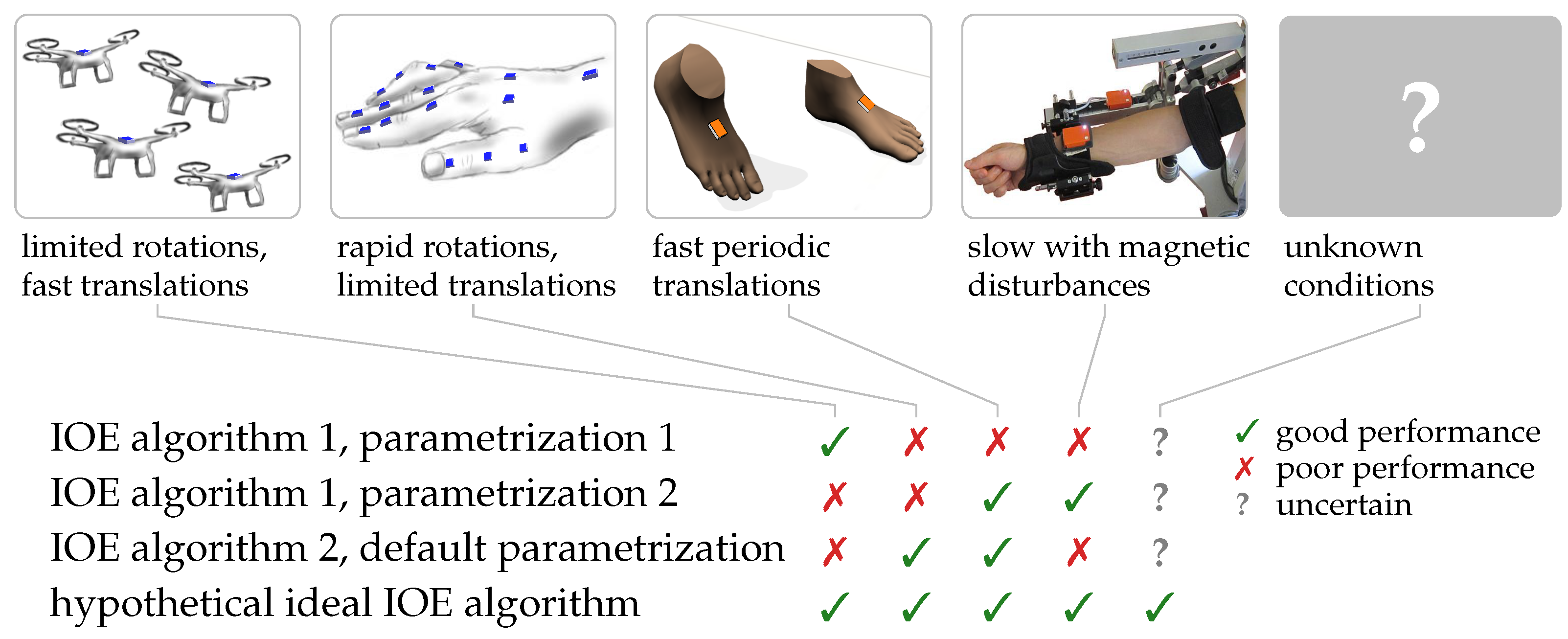
As illustrated in Figure 1, there is a general need for robust IOE algorithms that provide accurate orientation estimates and perform well for a broad range of motions without the need to manually adjust tuning parameters for each type of motion [16]. When it comes to assessing the performance of IOE algorithms, a vast number of contributions are found that evaluate specific algorithms in specific application contexts, but few papers investigate the ability of IOE algorithms to perform across different types of motion and environmental conditions. To the best of our knowledge, only Caruso et al. [9] provides a systematic evaluation of multiple algorithms with respect to three different movement speeds, and Fan et al. [17] investigates the influence of magnetic disturbances on the attitude and heading estimates. However, there are no studies providing a systematic and comprehensive evaluation of the impact of different magnetic disturbances, the difference between translational and rotational motions, and different movement speeds on various IOE algorithms.
As detailed in Section 2, a thorough algorithm comparison is limited by a lack of an extensive and openly available benchmark that includes a large number of trials comprising a diverse set of movement types and environmental conditions and therefore allows for a truly comprehensive evaluation and assessment of IOE solutions. Such a heterogeneous set of trials with either only rotation, only translation, or combined movements at different speeds and with different durations is important for two reasons. First, in order to assess the robustness of an IOE algorithm for a wide variety of motions and environmental conditions, those motions and conditions must be included in the data set. Second, comparing the errors for different trials yields insight into how algorithm performance or the choice of optimal parameters depends on the characteristics of the motion. As magnetic disturbances represent a major challenge in orientation estimation, it is crucial to not only consider homogeneous magnetic fields but to also include a broad range of magnetic disturbances.
The present contribution aims at filling this gap by providing a benchmark dataset that is particularly useful for the objective assessment and further development of IOE algorithms. To the best of our knowledge, this the first publicly available benchmark dataset that
- includes a broad range of different motions at various speeds
- contains separate trials with various deliberate magnetic disturbances
- contains separate trials with disturbances that affect the measured accelerations
- is already time-synchronized and contains ground truth data that requires no further preprocessing.
We further introduce error metrics that separately consider heading, inclination, and the total orientation error, specify well-defined benchmark metrics that can be used to assess and compare IOE algorithm performance, and provide example code to calculate those metrics.
The remainder of the article is structured as follows. In Section 2 we review a number of openly available datasets that are suitable for objective performance assessment of IOE algorithms. In Section 3 we present the new benchmark dataset and describe the contents and file structure. In Section 4 we describe the measurement setup, the performed data preprocessing, and introduce error metrics useful for quantifying the orientation estimation accuracy and define reproducible benchmark metrics. Section 5 is dedicated to applying some existing orientation estimation algorithms to the proposed benchmark. Conclusions are presented in Section 6.
2. Brief Review of Existing Datasets for IOE Validation
Objective assessment of the accuracy of an IOE algorithm requires a highly reliable and accurate ground truth measurement. The most widely accepted gold standard measurement for the orientation of a moving object is to derive its orientation from the position measurements of active or reflective optical markers that are tracked by a set of cameras, a technique that is known as stereophotogrammetry or optical motion capture (OMC). In the past two decades, a number of studies have been performed in which an IMU and optical markers are attached to moving objects, including human body segments, aerial vehicles, and robotic systems. While many of the datasets in these studies would be suitable for accuracy evaluation of IOE algorithms, the datasets are often not openly available or only available upon request to the authors, often due to privacy or ethical concerns. Furthermore, there is a lack of systematic benchmarking approaches for IOE accuracy evaluation. Despite this general lack of datasets and methods for evaluation, a few datasets have been made publicly available and are briefly reviewed in the following. Some of these datasets are created for general IOE validation and some are provided for evaluation in specific application contexts.
In total, we found five publicly available datasets that contain optical and inertial data from a moving object in a way that it allows for accuracy evaluation of an IOE algorithm. An overview of key features of the found datasets and the proposed dataset is given in Table 1.
In order to allow for evaluation of different aspects of an IOE algorithm, a useful universal benchmark dataset should fulfill a number of requirements. First and foremost, it should contain a large number of trials and a wide range of movements—including isolated translation and rotation movements—conducted at different speeds. To evaluate the robustness against magnetic disturbances, it is crucial to include both data recorded in a magnetically undisturbed environment and recordings with deliberate magnetic disturbances.
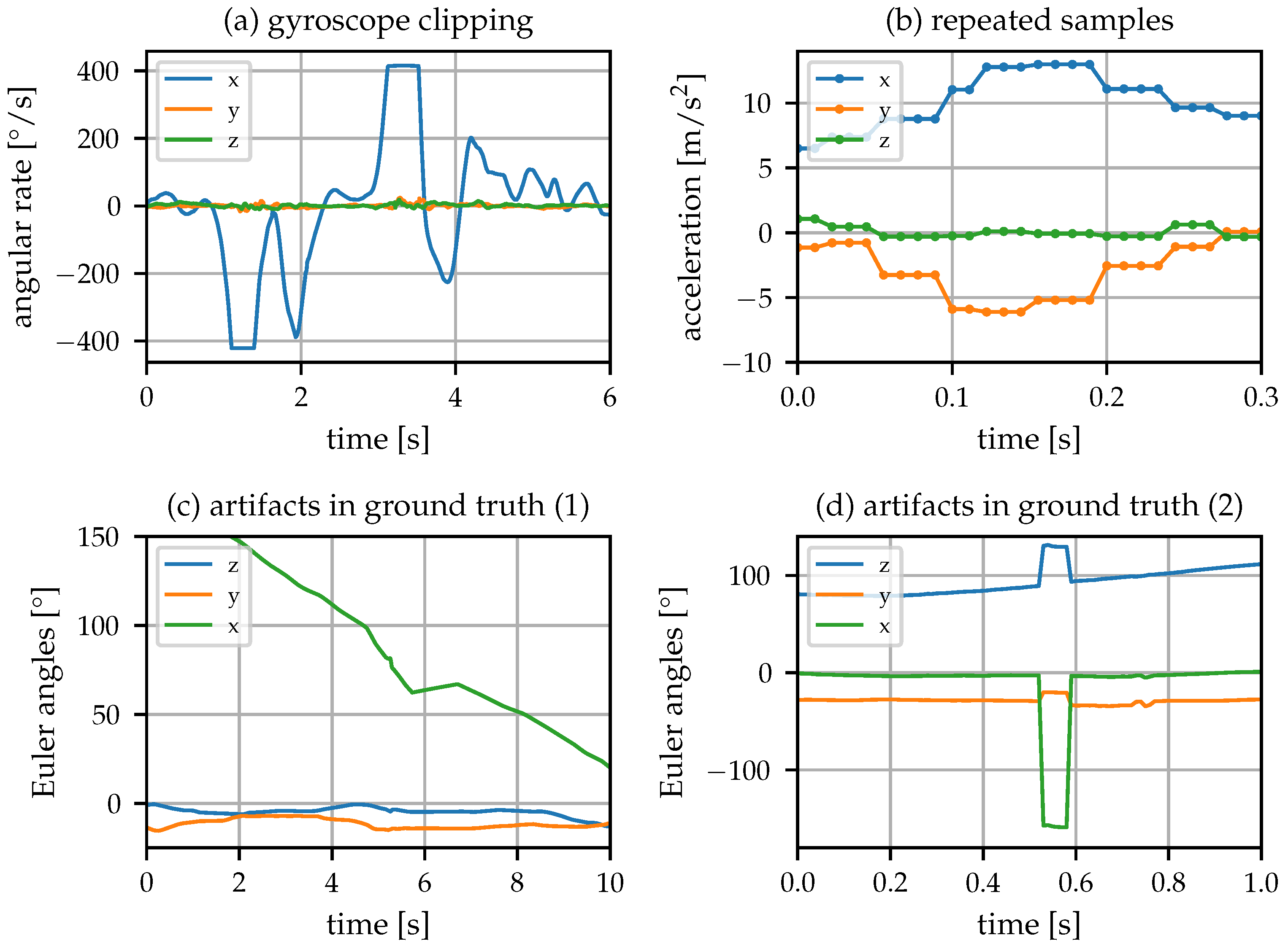
Furthermore, the quality of both the recorded IMU data as well as the ground truth OMC data is essential. In order to evaluate the performance in state-of-the-art applications, a state-of-the-art IMU with a sufficiently high sampling rate should be employed. Additionally, care should be taken to avoid artifacts due to errors in the reference system or in the recording of the IMU data. Figure 2 shows four examples of artifacts found in the publicly available datasets. The effects of such issues in the recorded data can often dominate the overall estimation error. In the best case, this makes the resulting observations less distinct and in the worst case, it could lead to wrong conclusions. Therefore, measurement data should be carefully checked before it is used for evaluation.
As can be seen in Table 1, each of the previously published datasets covers some of the mentioned aspects but none of them fulfill all previously mentioned requirements for a universal IOE benchmarking dataset. In the following, we will discuss each dataset in detail.
2.1. RepoIMU Dataset (T-Stick Trials)
To the best of our knowledge, the dataset RepoIMU [18] is, up to now, the only dataset aimed at IOE evaluation with a dedicated publication. The dataset consists of two distinct sets of trials, recorded with a T-stick and a pendulum.
The T-stick data consists of 29 trials with a duration of approximately 90 s each. As the name implies, the IMU is attached to a T-shaped stick equipped with six reflective markers. Each trial consists of either slow or fast rotation around one primary sensor axis or translation along one primary sensor axis. Data from an XSens MTi IMU and a Vicon Nexus OMC system is synchronized and provided at 100 Hz.
The authors explicitly state that the coordinate system of IMU and ground truth are not aligned and propose a method to compensate one of the two required rotations (cf. Section 4.2) by a method based on quaternion averaging. Unfortunately, some of the trials contain gyroscope clipping (Figure 2a) and artifacts in the ground truth orientation (Figure 2c) that have a significant effect on the obtained errors. Therefore, careful preprocessing and exclusion of some trials should be considered when using the dataset for IOE accuracy evaluation.
2.2. RepoIMU Dataset (Pendulum Trials)
The second part of the RepoIMU datasets consists of data from a triple pendulum on which IMUs are mounted. The measurement data is provided at 90 Hz or 166 Hz. However, the IMU data contains frequently repeated samples, as shown in Figure 2b. This is typically a result of artificial upsampling or transmission problems where lost samples get replaced by copying the last received sample and effectively reduces the sampling rate. The sampling rate that is obtained when repeated samples are discarded is around 25 Hz and 48 Hz for the accelerometer and gyroscope, respectively. Due to this fact, we cannot recommend using the pendulum trials for high precision IOE accuracy evaluation.
2.3. Sassari Dataset
The dataset published in [16] is targeted to the validation of a parameter-tuning approach based on the orientation difference of two IMUs of the same model. To facilitate this, six IMUs from three manufacturers (Xsens, APDM, Shimmer) are placed on one wooden board. Rotation around specific axes and free rotation around all axes are repeated at three different speeds. The data is synchronized and provided at 100 Hz. The local coordinate frames are aligned by precise manual placement. The authors clearly describe how they calculate the obtained error metrics, including a method of using the initial orientation to align the reference frames.
This makes the dataset valuable for validating IOE accuracy. The inclusion of different speeds and multiple IMU types increases the value of this dataset. However, all motions are performed in a homogeneous magnetic field and purely translational movements are not included. The total movement duration of all 3 trials is 168 s, with the longest movement phase lasting 30 s.
2.4. OxIOD Dataset
The Oxford Inertial Odometry Dataset (OxIOD) [20] is an extensive collection of inertial data recorded by smartphones (primarily an iPhone 7 Plus) at 100 Hz, consisting of 158 trials and covering a distance of over 42 km with an OMC ground truth being available for 132 trials. Being targeted for inertial odometry, it does not include isolated rotation and translation movements, which are useful for systematic assessment of IOE performance in various conditions, but instead covers a broad range of everyday motions.
Due to that different focus, some information (e.g., the alignment of the coordinate frames) is not described in detail. Furthermore, the ground truth orientation contains frequent irregularities (e.g., spikes in the orientation that are not accompanied by similar jumps in the IMU data, see Figure 2d for one example). In order to use this dataset for IOE assessment, careful preprocessing should be considered.
2.5. EuRoC MAV Dataset
The EuRoC MAV dataset [21] features indoor flight data of a micro aerial vehicle (MAV) and is aimed at visual-inertial 3D environment reconstruction. The six Vicon room trials offer a synchronized and aligned OMC-based ground truth and are suitable for IOE accuracy evaluation. Note that camera images and 3D point cloud data are also included, which are not relevant in the IOE context.
Magnetometer data are not included which limits the evaluation to the inclination component (cf. Section 5). It is noteworthy that due to the nature of the data, the motion mostly consists of horizontal translation and rotation around the vertical axis, and the inclination does not vary significantly throughout the trials. As the vibrations due to the flight are clearly visible in the raw accelerometer data, the EuRoC MAV dataset provides a unique test case for orientation estimation with disturbed accelerometer data.
Note that there is a similar but older dataset of the same research group [23]. However, the data files for this dataset do not seem to be available anymore (checked on 22 June 2021).
2.6. TUM VI Dataset
The TUM VI dataset [22] for visual-inertial odometry consists of 28 trials with a handheld object equipped with a camera and an IMU. Due to this application focus, most trials only include OMC ground truth data at the beginning and at the end of the trial. However, the six room trials include full OMC data and are suitable for IOE accuracy assessment.
Time synchronization is straightforward using provided time stamps, and the local and global coordinate systems of the OMC ground truth are aligned to the IMU frame (cf. Section 4.2). Similar to the EuRoC MAV data, the motion mostly consists of horizontal translation and rotation around the vertical axis, and magnetometer data is not included.
2.7. Summary
All reviewed datasets have in common that inertial measurements have been recorded alongside an optical ground truth. While some datasets [16,18] are specifically recorded for evaluating the accuracy of IOE algorithms, others [20,21,22] are recorded with a different focus but still contain the necessary data for this task. The datasets [16,18] contain recordings with isolated rotation and/or translation movements at different speeds, but the number of trials and the length of the movement duration is limited. As discussed above, trials with magnetic disturbances are crucial for objective performance evaluation of high-end IOE algorithms. However, none of the datasets contain recordings performed in deliberately and realistically disturbed magnetic fields.
Due to the described lack of a universal benchmark dataset, publications proposing new IOE algorithms commonly use data for evaluation that is only available to the respective authors (see, e.g., [24,25]) and the errors reported in different publications cannot be compared. We, therefore, conclude that there is a considerable need for an extensive benchmarking dataset for IOE accuracy assessment.
3. Dataset Description
We propose the Berlin Robust Orientation Estimation Assessment Dataset (BROAD). This benchmark dataset for orientation estimation consists of a diverse collection of trials, covering different movement types, speeds, and both undisturbed motions as well as motions with deliberate accelerometer disturbances as well as motions performed in the presence of magnetic disturbances. The dataset is publicly available at https://0-dx-doi-org.brum.beds.ac.uk/10.14279/depositonce-12033 (accessed on 22 June 2021) and also https://github.com/dlaidig/broad (accessed on 22 June 2021) under the terms of the CC-BY 4.0 license.
3.1. Trials
The proposed benchmark dataset consists of 39 trials. We distinguish the performed trials based on different criteria:
- the type of motion: rotation, translation, and combined (rotational and translational motions)
- the speed at which the motion was performed: slow and fast
- whether the trial consists of one uninterrupted continuous motion or of several segments with short breaks in between: no breaks, with breaks
- whether there are deliberate disturbances that affect the accelerometer measurements: undisturbed, tapping, and vibrating smartphone
- the magnetic environment in which the motion takes place: undisturbed (homogeneous indoor magnetic field), stationary magnet, attached magnet, office environment.
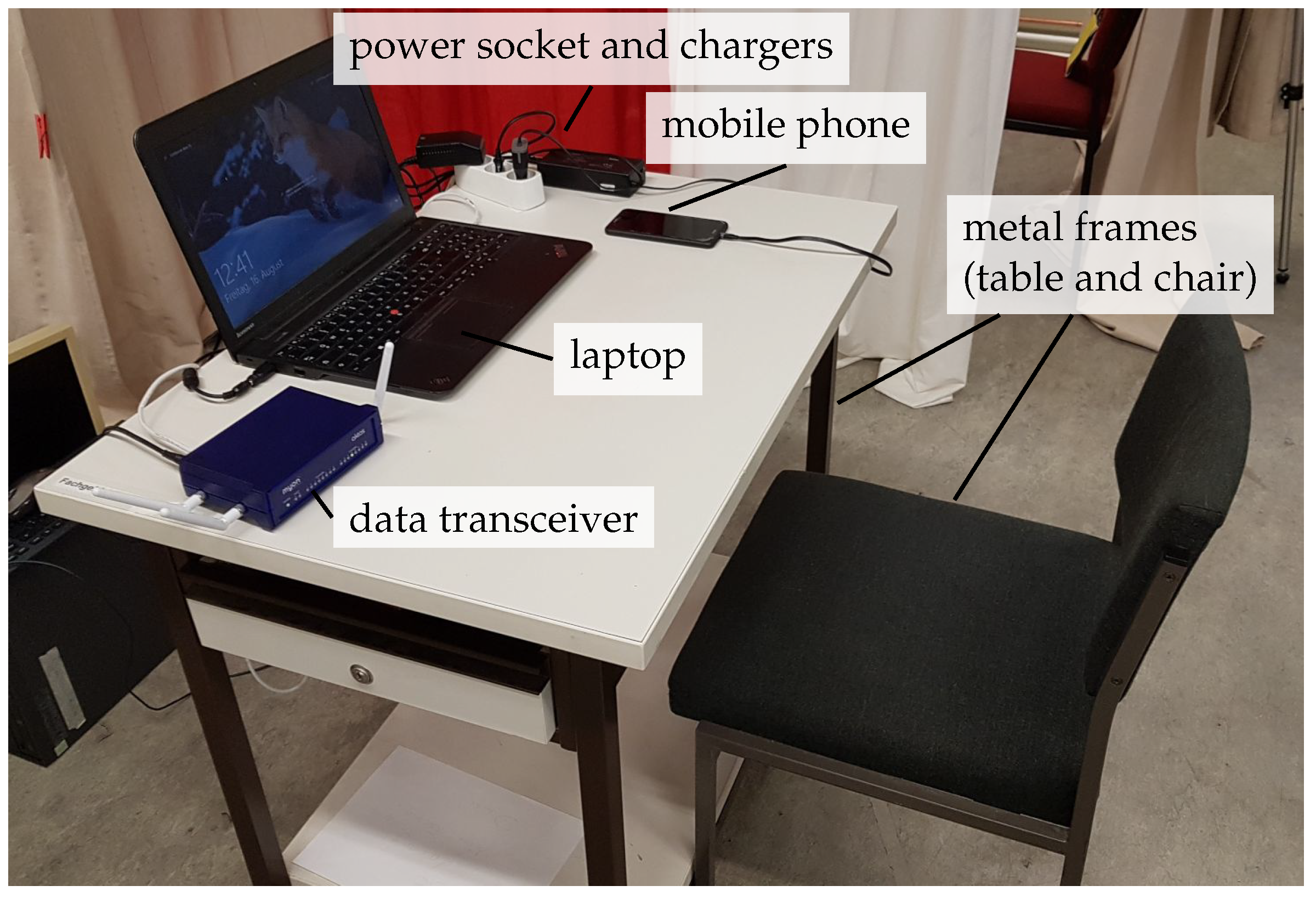
An overview of the performed trials can be found in Table 2. The considered disturbances are as follows. In the tapping trials, the IMU was repeatedly tapped using a finger, leading to spikes in the measured accelerations. In two trials, a vibrating smartphone was placed on the 3D-printed rigid body, causing significant high-frequency disturbances in the accelerometer measurements while at the same time disturbing the magnetometer measurements. In the stationary magnet trials, a small neodymium magnet was placed in the vicinity of the resting place, and part of the motion was deliberately performed close to the magnet. In the attached magnet trials, the magnet was placed on the rigid body at distances of 1, 2, 3, 4 and 5 cm. The office environment (Figure 3) consisted of various types of ferromagnetic material and electronic devices chosen to represent a typical indoor workplace environment. The mixed trial consisted of various short challenging motion phases, both disturbed and undisturbed.
All trials contain a rest phase of approximately 30 s at the beginning and at the end during which the rigid body with the IMU is resting on a table. A separate annotation signal in the provided data files shows whether the IMU is at rest or in motion. This annotation was performed manually based on plots of the measurement data.
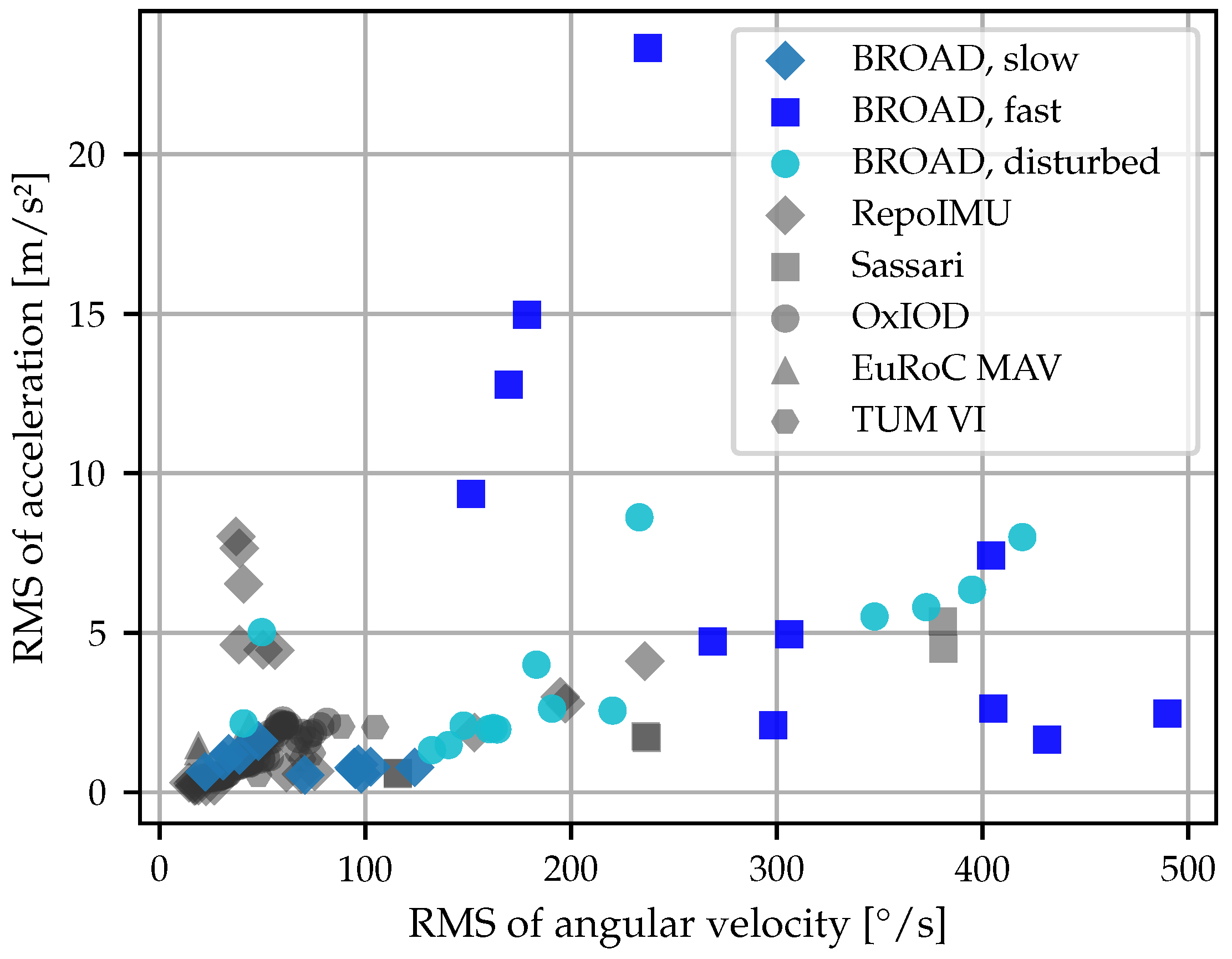
The 39 trials have a total duration of 8478 s when considering rest and motion phases and 5274 s when only considering phases with movement. The duration of a single motion phase ranges from 15 to 358 s. For the 39 trials, the root mean square (RMS) value of the angular velocity norm during motion ranges from 22 to 490°/s (slow trials: 22 to 124°/s, fast trials: 151 to 490°/s) with peak values (99th percentile) of up to 1116°/s. The RMS value of the acceleration norm (with 9.81 m/s2 removed) ranges from 0.5 to 23 m/s2 (slow trials: 0.5 to 1.6 m/s2, fast trials: 1.6 to 23 m/s2) with peak values (99th percentile) of up to 67 m/s2. The RMS values of all trials are shown in Figure 4 and cover a wider range than publicly available datasets.
3.2. File Format
The benchmark dataset consists of the 39 trials as presented in Table 2. Each trial is stored in a separate file, and the filename indicates the trial number and the type of trial (e.g., “01_undisturbed_slow_rotation_A”). A machine-readable “trials.json” file is included which can be used to automatically find and filter all trials.
The measurement data are provided both as an HDF5 data file and a Matlab data file (.mat) with identical content. Each file contains the following variables:
- imu_gyr IMU gyroscope measurements in rad/s
- imu_acc IMU accelerometer measurements in m/s2
- imu_mag IMU magnetometer measurements in
- opt_quat OMC ground truth orientation as a unit quaternion (w component first, ENU reference frame)
- opt_pos OMC ground truth position in m
- movement Boolean array (0/1) indicating movement phases
- sampling_rate sampling rate of the measurements in (, HDF5: stored as an attribute)
- info short description of the file contents (HDF5: stored as an attribute)
The data are already synchronized and aligned as described in Section 4.2. In order to obtain comparable results, orientation estimation algorithms should be run over the whole trial data but when calculating errors, the movement array should be used to exclude the rest phases.
3.3. Example Code
In addition to the measurement data, we provide example code written in Python. The code implements the evaluation and benchmark metrics described in Section 4.2 and Section 4.3, respectively, and re-creates Figures 8 and 9 from the case study in Section 5. Please refer to the information provided in the README.md file for instructions on how to run the code.
4. Materials and Methods
4.1. Hardware Setup
IMU data were recorded at a sampling rate of 286 using a commercially available nine-axis inertial sensor (myon aktos-t, myon AG, Schwarzenberg, Switzerland). Ground truth data at 120 were obtained via an Optitrack OMC system (NaturalPoint, Inc., Corvallis, OR, USA) consisting of eight Flex13 cameras.
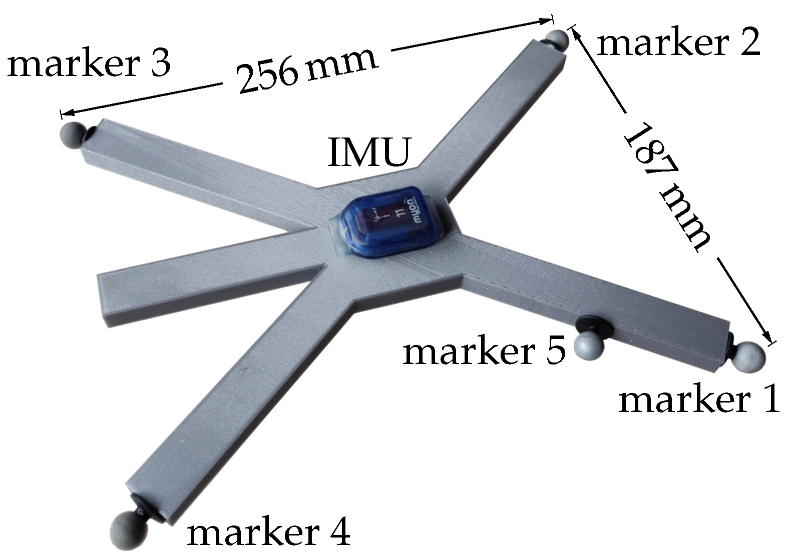
In order to ensure a highly precise ground truth orientation, the IMU and five reflective optical markers were placed on a rigid but lightweight 3D-printed structure, which is shown in Figure 5, with a minimum distance of 187 between any two corner markers. At those marker distances, the mean position accuracy of of the optical system corresponds to an angular orientation accuracy of approximately 0.2°.
The IMU input ranges were set to ±2000/s, g, and . In the recorded trials, turn-on gyroscope bias was found to be 0.17/s on average (per sensor axis), with 0.50/s being the maximum value. To simulate realistic conditions, this gyroscope bias is contained in the recorded data files. We determined further sensor characteristics (for each sensor axis) from a 49 recording of the IMU being at rest. The noise standard deviations in x, y, and z direction were found to be 0.10/s, 0.09/s, and 0.12/s for the gyroscope, /, /, and / for the accelerometer, and , , and for the magnetometer. The gyroscope random walk was ,
, and
(Allan deviation for observation time of 1 s), and the bias instability was
,
, and
(minimum Allan deviation).
4.2. Data Preprocessing
In order to create a benchmark dataset that is suitable for IOE accuracy evaluation, several preprocessing steps are needed. In the following section, we provide a high-level overview of the performed preprocessing steps as it is common practice in similar publications. Detailed descriptions are given in Appendix B and Appendix C.
Highly precise time synchronization of the IMU and OMC data streams is crucial because even very short time delays can have a significant effect on the observed orientation estimation errors. Synchronization was performed via optimization based on the measured angular velocity norm and an angular velocity derived from the OMC orientations. In addition to a time offset, a time drift correction factor was determined in order to account for small deviations from the nominal sampling frequencies of both measurement systems. The resulting parameters were used to interpolate the OMC ground truth data to the exact sampling time instants of the IMU data.
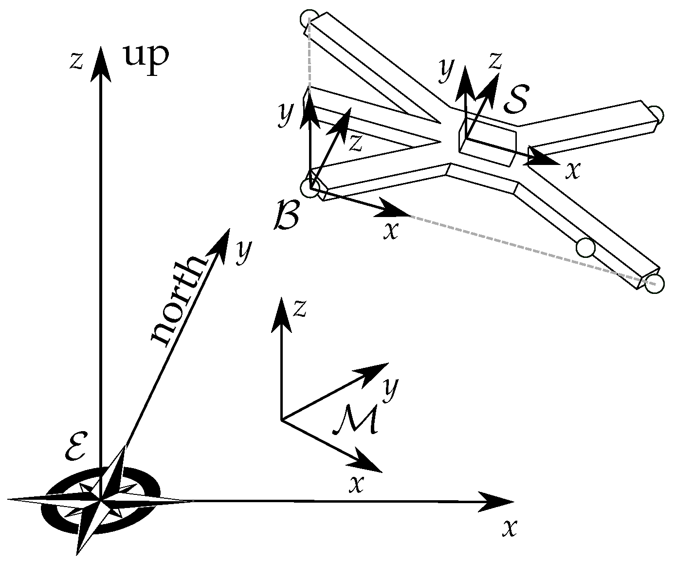
In order to obtain an accurate ground truth for the IMU orientation, the different local and global coordinate frames of both measurement systems have to be aligned [26]. See Figure 6 for an illustration of the different coordinate systems. The local coordinate systems of the IMU (determined by sensor manufacturing and calibration) and the rigid body (determined by the placement of optical markers) can agree well (<1) when care is taken to ensure precise placement, but even this small deviation might affect the results. The IMU reference frame is determined by gravity and the horizontal projection of the local Earth magnetic field. In contrast, OMC systems provide marker position measurements in a different reference frame that is defined by the camera positioning and a calibration procedure.
For a precise evaluation of the actual IOE errors, the constant offsets between and and between and must be determined [26]. This is done by minimizing the disagreement between the gyroscope and accelerometer measurements and corresponding quantities derived from the OMC measurement data. This alignment method is performed using a separate alignment recording that was performed on each measurement day. In those recordings, the IMU and the board are carefully and slowly rotated in all directions in order to ensure a sufficiently rich motion. The obtained alignment parameters are then used to calculate ground truth orientations from the OMC measurements of the 39 motion trials.
4.3. Metrics for Orientation Accuracy
For any of the performed motions, the orientation estimated by an IMU-based algorithm can be compared with the corresponding optical ground truth measurement. Along with the dataset, we provide example code to obtain the proposed metrics.
We use unit quaternions to represent rotations and orientations. For the convenience of the reader, the notation is briefly explained in Appendix A. The disagreement between two unit quaternions representing orientations is well described by the shortest angular distance e between both orientations. For any estimated sensor orientation and corresponding ground-truth orientation this error is
This angular performance parameter well describes the overall accuracy of the estimated orientation, and root-mean-square values can be used to quantify the performance of a motion interval of interest.
It is important to note that the error e yields only very limited insights into the potential cause of estimation errors. It is therefore highly desirable to distinguish between the portion of the error that results from inaccurate heading estimation as well as the portion that results from inaccurate inclination estimation. While the accuracy of the former depends primarily on the sensor fusion between gyroscopes and magnetometers, the accuracy of the latter primarily depends on sensor fusion between gyroscopes and accelerometers. In magnetically disturbed environments, the heading component of the error might easily be ten times larger than the inclination component of the orientation error.
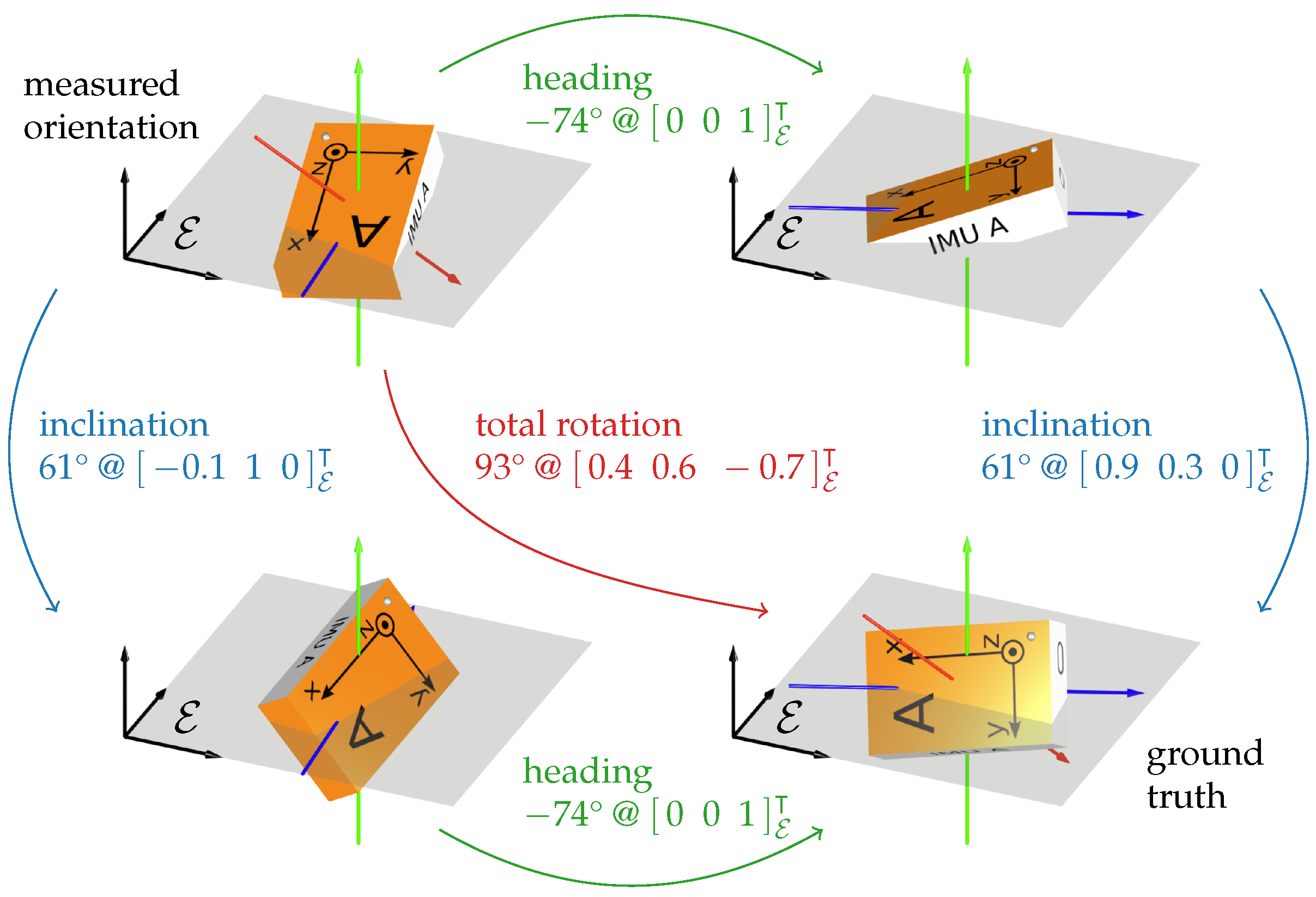
While different definitions of heading have been used in the literature, we use a heading/inclination decomposition of quaternions that is particularly useful for the current purpose. The rotation between any given two orientations can always be decomposed into a rotation around the vertical axis and a rotation around a horizontal axis, as illustrated in Figure 7. We call the first rotation heading and the second rotation inclination. Note that this is not equivalent to the decomposition based on Euler angles as proposed, e.g., in [27]. In that decomposition, the inclination quaternion is a concatenation of two rotations and, in general, the rotation axis of that inclination quaternion is not horizontal. The decomposition proposed in Figure 7 does not exhibit this disadvantage.
To implement the desired decomposition, the following two steps are carried out. First, we express the orientation error in the global frame as follows.
We then decompose the orientation error into a rotation around the vertical z-axis and the shortest possible residual rotation. The absolute rotation angle of the former is called the heading error and the absolute rotation angle of the latter is called the inclination error . Analytic expressions for those errors can be derived by expressing the residual inclination rotation quaternion as a function of the heading rotation angle and then maximizing the w-component of this residual quaternion. This leads to the following definitions:
The proposed decomposition facilitates the interpretation of the overall estimation error with respect to potential sources of inaccuracy when comparing the orientations obtained by an IOE algorithm to the OMC ground truth. In general, large inclination errors indicate non-ideal fusion of accelerometer with gyroscope measurements while large heading errors are mostly caused by magnetic disturbances. The error is a suitable metric for the overall orientation estimation error. The sum of both error portions is always larger or equal to the overall orientation error while each portion for itself is smaller than that overall error.
Note that for the special case of orientation estimation from gyroscope and accelerometer measurements only, absolute heading information is not available. While, in this case, the heading error has a large offset and exhibits a slow drift, the inclination error is a suitable metric for assessing the accuracy of magnetometer-free IOE algorithms.
We can use the previously defined error metrics , , and , which are defined for each time instant, to assess the performance of a given IOE algorithm in different scenarios. In order to assess the overall performance for one trial, we use the root mean square error (RMSE) of the respective metric while only considering the motion phases (as labeled in the data files). When considering a set of trials, we report the mean of the RMSE values obtained for each trial as a metric for the overall accuracy. In both cases, small RMSE values indicate good performance.
4.4. Benchmark Metrics
In order to allow for a simple and well-defined performance comparison between different IOE algorithms, we define two benchmark metrics that can be obtained from the BROAD dataset for any given IOE algorithm: the trial-agnostic generalized performance (TAGP) and the individual trial-optimized performance (ITOP). Both metrics are based on the average RMSE that is obtained as follows:
- run the IOE algorithm on all 39 trials with a given parameter setting
- for each trial, calculate the orientation RMSE (i.e., the RMS of ) while only considering the labeled motion phases
- average all 39 RMSE values.
The TAGP is the smallest achievable average RMSE over all 39 trials that can be obtained with a common parameter setting for all trials. The ITOP is the smallest achievable average RMSE over all 39 trials that can be obtained with individual parameter tuning for each trial.
In Section 5 we will demonstrate how to obtain those metrics and how to use the proposed benchmark for further in-depth evaluation.
5. Case Study on the Proposed Benchmark Dataset
In the following exemplary case study, we demonstrate the usefulness of the proposed benchmark and show how it can be employed to achieve an objective and broad assessment and comparison of IOE algorithms under different conditions by answering several exemplary research questions. To this end, we evaluate the performance of two popular orientation estimation algorithms, the complementary filters proposed in [24] (Algorithm A) and [28] (Algorithm B). For both filters, we employ the commonly used C implementation by Sebastian Madgwick (https://x-io.co.uk/open-source-imu-and-ahrs-algorithms/, accessed on 22 June 2021).
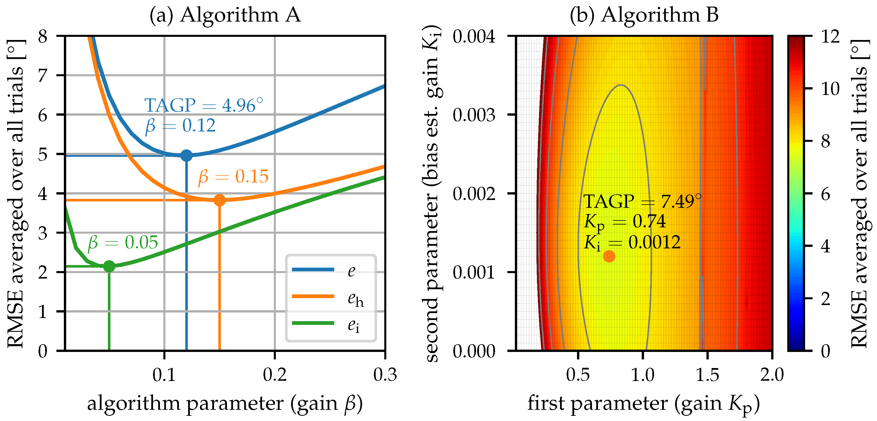
Consider orientation estimation in an application setting in which we do not have knowledge regarding speed and type of motions and in which we cannot guarantee an undisturbed environment. Our aim is to find robust parameter settings for Algorithms A and B that minimize the average error over all possible scenarios. This specific research question is equivalent to finding the parameter settings associated with the TAGP. In order to determine this value, we calculate the average RMSE as defined in Section 4.4 for many different parameter values. For Algorithm A, we use linearly spaced values of the single tuning parameter (0.01 to 0.3 in steps of 0.01). As Algorithm B has two tuning parameters, a fusion weight (similar to ) and a parameter for gyroscope bias estimation , we search a linearly spaced grid of parameter values (: 0.02 to 2.0 in steps of 0.02, : 0 to 0.004 in steps of 0.0001). The result is shown in Figure 8. We can see that, for this broad range of motions, a value of yields the lowest overall errors for Algorithm A and that for Algorithm B the lowest overall error is obtained for the parameter combination is , .
Besides this research question, the details presented in Figure 8a can be used to answer various minor research questions: Consider an application for which only the inclination error is relevant and therefore should be minimized. As can be seen in Figure 8a, should be chosen for this case. Analogously, we see that accurate heading estimation requires larger values for , with the optimum being at . The line plot representation also allows us to answer the question of how non-ideal values for influence the error: We can see that the error gradient is much steeper when is too small than when it is too large, i.e., if in doubt, larger values for should be chosen.
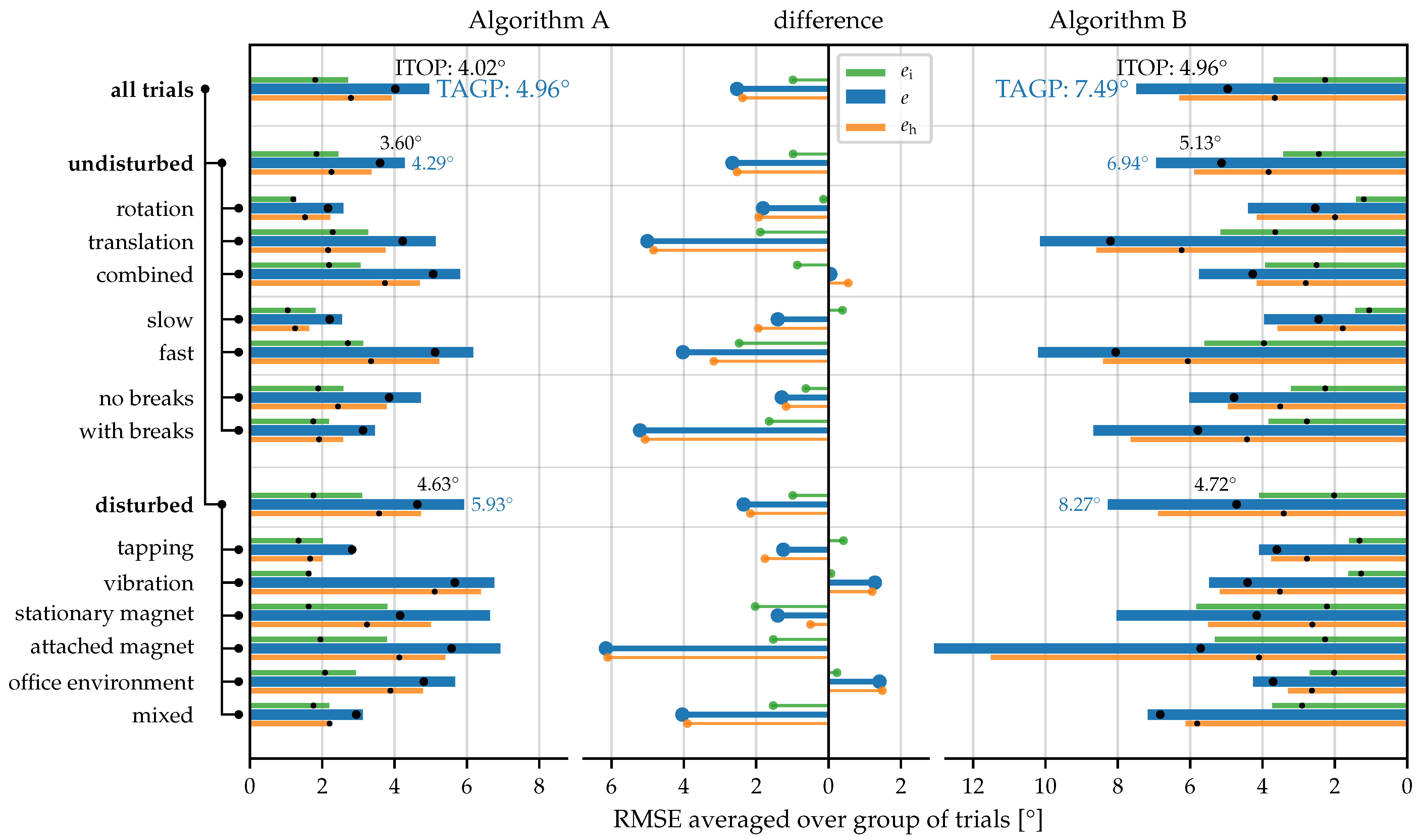
In order to take an in-depth look at the strengths and weaknesses of a given IOE algorithm, we pose the following research question: How does the estimation accuracy of Algorithms A and B depend on the type of motion and environmental conditions? Unlike available datasets, the BROAD benchmark is well suited for answering this question. This can be achieved for example as follows. We calculate the average inclination, heading, and total RMSE for the groups of trials as defined in Table 2 with the TAGP parametrization. Furthermore, we determine the minimum achievable error when using ideal parameters for each trial. In Figure 9 the TAGP performance is shown with bars, and the minimum achievable error is indicated with black dots.
We see that for the TAGP benchmark metric, Algorithm A reaches a score of 4.96° and Algorithm B reaches a score of 7.49°, i.e., Algorithm A yields a better overall performance. Furthermore, the breakdown into trial groups allows for a detailed evaluation of the estimation accuracy in various scenarios. For example, we can see that, for both algorithms, pure rotational movements yield lower errors than translational movements. For Algorithm A, the error for combined motions is larger than for translational movements while for Algorithm B the error obtained for combined motions is smaller than for pure translational movements. Unsurprisingly, faster movements lead to larger errors with both algorithms. As can be seen in Figure 9, the estimation errors do not show any notable difference between long continuous movement phases and short phases with breaks in between. The decomposition into heading and inclination error in combination with the magnetic disturbances included in the dataset allows for insight into potential sources of errors. In the undisturbed trials, heading and inclination almost equally contribute to the total error, while for the attached-magnet trials and Algorithm B, the heading error is twice as large as the inclination error.
Combining the results of the two algorithms in Figure 9 enables us to easily answer another research question: Which of the algorithms provides the best overall accuracy and which algorithm is more accurate for any given motion scenario? To further facilitate the comparison of the algorithm performance, we plot the error difference for each group of trials as lines originating from the center of Figure 9. We see that when using the common robust parameter settings, the performance of Algorithm A is better than the performance of Algorithm B when considering the average performance of all trials. Algorithm A also yields lower or almost equal errors for most trial groups except for the vibration and office environment trials, where the performance of Algorithm B is better.
The differences between TAGP and ITOP performance allow us to answer another research question: How well do algorithms A and B generalize, i.e., can they provide near-optimum performance for a wide variety of motions with a single common parameter choice? The ability to generalize is a desirable property since individual parameter tuning depending on the expected motion is often not possible in practice [16]. In Figure 9, we see that for Algorithm B the ITOP errors are much smaller than the TAGP errors whereas for Algorithm A the difference between individually tuning and a common parameter choice is much smaller. This shows that there is more potential for parameter tuning with Algorithm B while Algorithm A generalizes better.
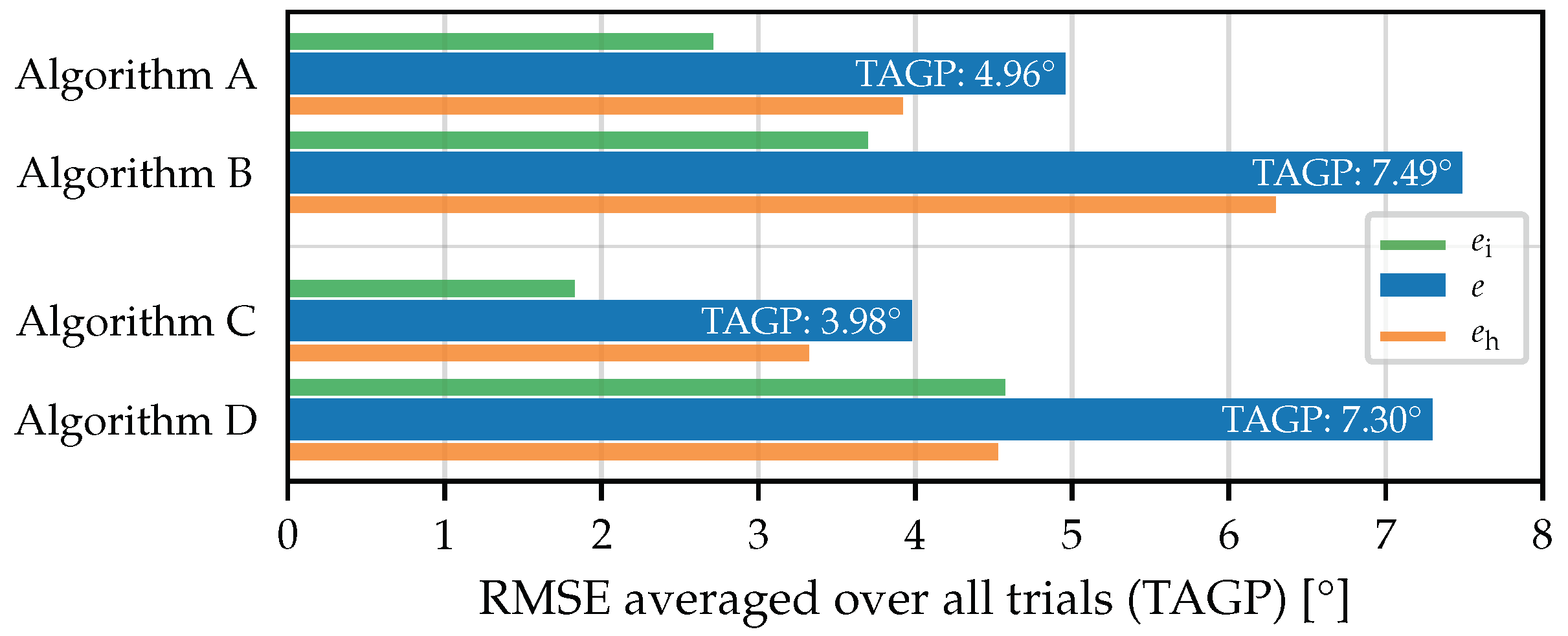
As a final research question, we aim to determine how well the two considered IOE algorithms perform compared to other state-of-the-art algorithms. Since Algorithm A and B are complementary filters, we choose two algorithms based on Kalman filters for which an implementation is available in [9]: the method proposed by Ligorio and Sabatini [29] (Algorithm C, LIG in [9]) that yielded the best performance in [9] and the computationally efficient method proposed by Guo et al. [30] (Algorithm D, GUO in [9]). To answer this question, we determine the benchmark metric TAGP for all algorithms.
The results are shown in Figure 10. As can be seen, Algorithm D yields an overall performance that is very similar to the performance of Algorithm B. With a TAGP of 3.98°, Algorithm C provides the best overall performance and outperforms Algorithm A by around 1°. The breakdown of the TAGP into heading and inclination components shows that, while the errors are lower for both heading and inclination, a larger part of the overall improvement can be attributed to more accurate inclination estimates.
6. Conclusions
The validation of novel IOE algorithms is typically performed with not-openly-available application-specific datasets that only contain certain types of motions. This makes it difficult to compare performance across different algorithms, to gain insight into the robustness of different algorithms in a broad range of scenarios, and to investigate the influence of tuning parameters. There is a lack of publicly available datasets that are suitable for robust IOE accuracy evaluation.
The proposed BROAD benchmark contributes towards filling this gap. In contrast to previously published datasets, it encompasses a wide range of undisturbed motions as well as motions in disturbed environments. As shown in the exemplary case study with two widely used orientation estimation algorithms, this benchmark dataset allows for
- the determination of robust algorithm parameters for a given IOE algorithm that perform well for a broad range of motions and environmental conditions,
- an in-depth analysis of strength and weaknesses of a given IOE algorithm in different scenarios, while considering heading and inclination separately,
- a detailed comparison of the performance of different algorithms with respect to a wide range of possible application and motion scenarios,
- an objective comparison of different literature algorithms as well as targeted development of new algorithms with improved performance by using the well-defined benchmark metrics described in Section 4.4.
The exemplary case study is by no means comprehensive and there are many further possibilities for using the benchmark dataset. This includes the assessment of online gyroscope bias estimation methods, for which gyroscope turn-on bias at different realistic magnitudes could be added to the data, as well as evaluation of different magnetic disturbance rejection approaches.
The BROAD benchmark is particularly useful for the objective assessment of IOE algorithms across different types of motions and environmental conditions and is therefore expected to contribute to the advancement of IMU-based motion analysis.
To further broaden the development of robust and accurate IOE algorithms for human motion analysis, future research will aim at complementing the BROAD dataset by adding existing or newly recording data from human motion trials with a reliable, synchronized, and aligned optical ground truth. Furthermore, future research will aim at providing benchmark measurements obtained with different IMU hardware, and at using the benchmark to develop and validate IOE algorithms.
Author Contributions
Conceptualization, D.L. and T.S.; methodology, D.L. and T.S.; software, D.L. and M.C.; validation, D.L. and M.C.; formal analysis, D.L. and T.S.; investigation, D.L.; resources, T.S.; data curation, D.L.; writing—original draft preparation, D.L.; writing—review and editing, D.L., M.C., A.C. and T.S.; visualization, D.L.; supervision, T.S.; project administration, T.S.; funding acquisition, T.S. All authors have read and agreed to the published version of the manuscript.
Funding
We acknowledge support by the German Research Foundation and the Open Access Publication Fund of TU Berlin.
Institutional Review Board Statement
Not applicable.
Informed Consent Statement
Not applicable.
Data Availability Statement
Data and example code is provided at https://0-dx-doi-org.brum.beds.ac.uk/10.14279/depositonce-12033 as well as https://github.com/dlaidig/broad under the terms of the CC-BY 4.0 license.
Acknowledgments
We thank Kai Brands for his skillful support in conducting the experiments and processing the data.
Conflicts of Interest
The authors declare no conflict of interest.
Abbreviations
The following abbreviations are used in this manuscript:
| BROAD | Berlin robust orientation estimation assessment dataset |
| IMU | inertial measurement unit |
| IOE | inertial orientation estimation |
| MAV | micro aerial vehicle |
| OMC | optical motion capture |
| RMSE | root mean square error |
Appendix A. Quaternion Notation
Unit quaternions in vector notation are used to represent rotations and orientations [31]. We denote quaternion multiplication by ⊗ and, to simplify the notation, implicitly regard three-dimensional vectors as quaternions with zero real part. When a quaternion is used to represent orientations, left upper and lower indices are used to indicate the coordinate frames. For example, we denote the IMU orientation commonly reported by IOE algorithms as , i.e., the rotation from an inertial reference frame to the coordinate system of the sensor .
Appendix B. Time Synchronization
As both the IMU measurement and the OMC recording were started and stopped manually and both systems record data at different sampling rates, the measurements need to be time-synchronized. We obtain this by the following procedure:
Denote the sampling time of the IMU as and the sampling time of the OMC system as . First, we derive a optical angular velocity from the optical orientation :
We then low-pass filter each component of the inertial angular velocity and the optical angular velocity with a cutoff frequency of 10 .
By nonlinear least-squares optimization, we determine the time offset and the scaling factor s of the nominal OMC sampling rate that minimizes the RMSE between the norms of both angular rates, i.e.,
with
To ensure robust convergence, we first determine an initial estimate of the time offset by evaluating this cost function with time offsets at a regular interval. In a second step, we parametrize an additional offset and the clock scaling as a time shift at the beginning and at the end of the measurement.
As the final step, we use the obtained time shift and OMC sampling rate to resample the measured OMC data to the IMU sampling instants.
Appendix C. Coordinate System Alignment
While the IMU-based IOE algorithms yield the orientation of the sensor coordinate system with respect to a frame of reference defined by the vertical direction and the local magnetic field, the optical system determines the orientation of the marker cluster with respect to an internal reference coordinate system . This is illustrated in Figure 6.
Note that the rotation between the frame and the frame and the rotation between the frame and the frame are constant throughout the entire duration of the motion and only depend on the installation of the markers and the calibration of the optical ground truth system as well as the local magnetic field inside the room and the attachment of the IMU on the rigid body. To evaluate whether the orientation that is estimated by the IMU-based method is accurate, the frame and the frame as well as the frame and the frame must be aligned with each other so that the IMU-based orientation can be compared with the ground truth measurement. We now explain how the rotation between and and between frame and the can be determined based on any measurement that contains inertial and optical data from a sufficiently rich motion.
Assume that the inertial and optical data is already synchronized by the method described in Appendix B. During this synchronization, we deliberately only considered the norm of the optical angular velocity and the gyroscope measurements , as the 3D vectors are given in the local coordinate systems and , respectively. We can exploit the direction of those vectors to determine the relative orientation . When also considering a fixed gyroscope bias , it can be expected that the correct minimizes the following cost function:
Using the central second-order finite difference, we derive an optical acceleration signal from the OMC position measurements. In order to make this measurement agree with the IMU accelerometer measurements, knowledge of both and is needed. In the frame, the measured gravitational acceleration is , with a fixed but unknown . We express the IMU accelerometer measurements in the frame using the OMC orientation :
denotes an unknown but constant accelerometer bias. Using those quantities, we define the following cost function:
We can then determine the parameters , , , , and g that minimize the sum of both cost functions, i.e., . Note that for a unique solution, we set the z-component of to zero, which ensures a consistent heading. To increase robustness, we low-pass filter the optical and inertial measurements with a cutoff frequency of 10 . This problem can be solved by standard nonlinear optimization methods. It is generally well-behaved, and the solution is straightforward to find.
The heading component of is determined in a second step: We transform the magnetometer measurements in the frame using the OMC orientation and the results from the previous step and, for each sample, calculate the angle of the measurement in the horizontal plane. Finally, the mean of the obtained heading angles is used to determine the heading of .
References
- Seel, T.; Kok, M.; McGinnis, R.S. Inertial Sensors—Applications and Challenges in a Nutshell. Sensors 2020, 20, 6221. [Google Scholar] [CrossRef] [PubMed]
- Passon, A.; Schauer, T.; Seel, T. Inertial-Robotic Motion Tracking in End-Effector-Based Rehabilitation Robots. Front. Robot. AI 2020, 7. [Google Scholar] [CrossRef] [PubMed]
- Kotiadis, D.; Hermens, H.J.; Veltink, P.H. Inertial Gait Phase Detection for Control of a Drop Foot Stimulator: Inertial Sensing for Gait Phase Detection. Med. Eng. Phys. 2010, 32, 287–297. [Google Scholar] [CrossRef]
- Seel, T.; Laidig, D.; Valtin, M.; Werner, C.; Raisch, J.; Schauer, T. Feedback Control of Foot Eversion in the Adaptive Peroneal Stimulator. In Proceedings of the 22nd Mediterranean Conference on Control and Automation, Palermo, Italy, 16–19 June 2014; pp. 1482–1487. [Google Scholar] [CrossRef] [Green Version]
- Nguyen, H.; Lebel, K.; Bogard, S.; Goubault, E.; Boissy, P.; Duval, C. Using Inertial Sensors to Automatically Detect and Segment Activities of Daily Living in People with Parkinson’s Disease. IEEE Trans. Neural Syst. Rehabil. Eng. 2018, 26, 197–204. [Google Scholar] [CrossRef]
- Werner, C.; Schneider, S.; Gassert, R.; Curt, A.; Demkó, L. Complementing Clinical Gait Assessments of Spinal Cord Injured Individuals Using Wearable Movement Sensors. In Proceedings of the 2020 42nd Annual International Conference of the IEEE Engineering in Medicine Biology Society (EMBC), Montreal, QC, Canada, 20–24 July 2020; pp. 3142–3145. [Google Scholar] [CrossRef]
- Woodman, O.J. An Introduction to Inertial Navigation; Technical Report UCAM-CL-TR-696; Computer Laboratory, University of Cambridge: Cambridge, UK, 2007. [Google Scholar]
- Kok, M.; Hol, J.D.; Schön, T.B. Using Inertial Sensors for Position and Orientation Estimation. Found. Trends® Signal Process. 2017, 11, 1–153. [Google Scholar] [CrossRef] [Green Version]
- Caruso, M.; Sabatini, A.M.; Laidig, D.; Seel, T.; Knaflitz, M.; Della Croce, U.; Cereatti, A. Analysis of the Accuracy of Ten Algorithms for Orientation Estimation Using Inertial and Magnetic Sensing under Optimal Conditions: One Size Does Not Fit All. Sensors 2021, 21, 2543. [Google Scholar] [CrossRef]
- Nazarahari, M.; Rouhani, H. 40 Years of Sensor Fusion for Orientation Tracking via Magnetic and Inertial Measurement Units: Methods, Lessons Learned, and Future Challenges. Inf. Fusion 2020. [Google Scholar] [CrossRef]
- Weber, D.; Guehmann, C.; Seel, T. Neural Networks Versus Conventional Filters for Inertial-Sensor-Based Attitude Estimation. In Proceedings of the 2020 IEEE 23rd International Conference on Information Fusion (FUSION), Rustenburg, South Africa, 6–9 July 2020. [Google Scholar]
- Caruso, M.; Sabatini, A.M.; Knaflitz, M.; Gazzoni, M.; Croce, U.D.; Cereatti, A. Accuracy of the Orientation Estimate Obtained Using Four Sensor Fusion Filters Applied to Recordings of Magneto-Inertial Sensors Moving at Three Rotation Rates. In Proceedings of the 2019 41st Annual International Conference of the IEEE Engineering in Medicine and Biology Society (EMBC), Berlin, Germany, 23–27 July 2019; pp. 2053–2058. [Google Scholar] [CrossRef]
- de Vries, W.H.K.; Veeger, H.E.J.; Baten, C.T.M.; van der Helm, F.C.T. Magnetic Distortion in Motion Labs, Implications for Validating Inertial Magnetic Sensors. Gait Posture 2009, 29, 535–541. [Google Scholar] [CrossRef]
- Ligorio, G.; Sabatini, A.M. Dealing with Magnetic Disturbances in Human Motion Capture: A Survey of Techniques. Micromachines 2016, 7, 43. [Google Scholar] [CrossRef] [PubMed] [Green Version]
- Fan, B.; Li, Q.; Wang, C.; Liu, T. An Adaptive Orientation Estimation Method for Magnetic and Inertial Sensors in the Presence of Magnetic Disturbances. Sensors 2017, 17, 1161. [Google Scholar] [CrossRef]
- Caruso, M.; Sabatini, A.M.; Knaflitz, M.; Gazzoni, M.; Croce, U.D.; Cereatti, A. Orientation Estimation through Magneto-Inertial Sensor Fusion: A Heuristic Approach for Suboptimal Parameters Tuning. IEEE Sens. J. 2021, 21, 3408–3419. [Google Scholar] [CrossRef]
- Fan, B.; Li, Q.; Liu, T. How Magnetic Disturbance Influences the Attitude and Heading in Magnetic and Inertial Sensor-Based Orientation Estimation. Sensors 2018, 18, 76. [Google Scholar] [CrossRef] [PubMed] [Green Version]
- Szczęsna, A.; Skurowski, P.; Pruszowski, P.; Pęszor, D.; Paszkuta, M.; Wojciechowski, K. Reference Data Set for Accuracy Evaluation of Orientation Estimation Algorithms for Inertial Motion Capture Systems. In Computer Vision and Graphics; Chmielewski, L.J., Datta, A., Kozera, R., Wojciechowski, K., Eds.; Lecture Notes in Computer Science; Springer International Publishing: Cham, Switzerland, 2016; pp. 509–520. [Google Scholar] [CrossRef]
- Jędrasiak, K.; Daniec, K.; Nawrat, A. The Low Cost Micro Inertial Measurement Unit. In Proceedings of the 2013 IEEE 8th Conference on Industrial Electronics and Applications (ICIEA), Melbourne, Australia, 19–21 June 2013; pp. 403–408. [Google Scholar] [CrossRef]
- Chen, C.; Zhao, P.; Lu, C.X.; Wang, W.; Markham, A.; Trigoni, N. OxIOD: The Dataset for Deep Inertial Odometry. arXiv 2018, arXiv:1809.07491. [Google Scholar]
- Burri, M.; Nikolic, J.; Gohl, P.; Schneider, T.; Rehder, J.; Omari, S.; Achtelik, M.W.; Siegwart, R. The EuRoC Micro Aerial Vehicle Datasets. Int. J. Robot. Res. 2016, 35, 1157–1163. [Google Scholar] [CrossRef]
- Schubert, D.; Goll, T.; Demmel, N.; Usenko, V.; Stückler, J.; Cremers, D. The TUM VI Benchmark for Evaluating Visual-Inertial Odometry. In Proceedings of the 2018 IEEE/RSJ International Conference on Intelligent Robots and Systems (IROS), Madrid, Spain, 1–5 October 2018; pp. 1680–1687. [Google Scholar] [CrossRef] [Green Version]
- Lee, G.H.; Achtelik, M.; Fraundorfer, F.; Pollefeys, M.; Siegwart, R. A Benchmarking Tool for MAV Visual Pose Estimation. In Proceedings of the 2010 11th International Conference on Control Automation Robotics & Vision, Singapore, 7–10 December 2010; pp. 1541–1546. [Google Scholar] [CrossRef] [Green Version]
- Madgwick, S.O.H.; Harrison, A.J.L.; Vaidyanathan, R. Estimation of IMU and MARG Orientation Using a Gradient Descent Algorithm. In Proceedings of the 2011 IEEE International Conference on Rehabilitation Robotics, Zurich, Switzerland, 29 June–1 July 2011; pp. 1–7. [Google Scholar] [CrossRef]
- Sabatini, A.M. Kalman-Filter-Based Orientation Determination Using Inertial/Magnetic Sensors: Observability Analysis and Performance Evaluation. Sensors 2011, 11, 9182–9206. [Google Scholar] [CrossRef] [PubMed]
- Hol, J.D. Sensor Fusion and Calibration of Inertial Sensors, Vision, Ultra-Wideband and GPS. Ph.D. Thesis, Linköping University, Linköping, Sweden, 2011. [Google Scholar]
- Bergamini, E.; Ligorio, G.; Summa, A.; Vannozzi, G.; Cappozzo, A.; Sabatini, A.M. Estimating Orientation Using Magnetic and Inertial Sensors and Different Sensor Fusion Approaches: Accuracy Assessment in Manual and Locomotion Tasks. Sensors 2014, 14, 18625–18649. [Google Scholar] [CrossRef] [PubMed] [Green Version]
- Mahony, R.; Hamel, T.; Pflimlin, J.M. Nonlinear Complementary Filters on the Special Orthogonal Group. IEEE Trans. Autom. Control 2008, 53, 1203–1218. [Google Scholar] [CrossRef] [Green Version]
- Ligorio, G.; Sabatini, A.M. A Novel Kalman Filter for Human Motion Tracking With an Inertial-Based Dynamic Inclinometer. IEEE Trans. Biomed. Eng. 2015, 62, 2033–2043. [Google Scholar] [CrossRef] [PubMed]
- Guo, S.; Wu, J.; Wang, Z.; Qian, J. Novel MARG-Sensor Orientation Estimation Algorithm Using Fast Kalman Filter. J. Sens. 2017, 2017, e8542153. [Google Scholar] [CrossRef] [Green Version]
- Kuipers, J.B. Quaternions and Rotation Sequences. In Proceedings of the International Conference on Geometry, Integrability and Quantization, Varna, Bulgaria, 1–10 September 1999; Coral Press Scientific Publishing: Sofia, Bulgaria, 2000; pp. 127–143. [Google Scholar] [CrossRef]
Figure 1.
The accuracy of inertial orientation estimation (IOE) depends on the employed algorithm, the chosen algorithm parametrization, and the specific application scenario. There is a lack of datasets and methods for systematic evaluation of IOE algorithm performance across a broad range of motion characteristics and environmental conditions.

Figure 2.
Examples of artifacts found in existing datasets. (a) Gyroscope clipping leading to large errors in angular rate strapdown integration. (b) Repeated samples in IMU data, leading to a very low effective sampling rate. (c,d) Two examples of artifacts found in the OMC ground truth orientations, potentially caused by interpolation of gaps and swapped markers.

Figure 3.
Office environment used to provide a realistic indoor scenario with magnetic disturbances.
Figure 3.
Office environment used to provide a realistic indoor scenario with magnetic disturbances.

Figure 4.
RMS values of the angular velocity and accelerometer norm for the undisturbed slow, undisturbed fast, and disturbed trials of the proposed dataset in comparison to the publicly available datasets (only considering trials suitable for IOE accuracy evaluation, cf. Section 2). The BROAD dataset covers a wider range of motions than publicly available datasets.

Figure 5.
Custom 3D-printed rigid body used in the experiments. The IMU is attached to the
center of the board using tape. Four reflective optical markers are attached to the ends of the Xshaped
structure to increase the distance between markers. A fifth marker is used to ensure that the
orientation can uniquely be determined from the marker positions.

Figure 6.
Illustration of the different local coordinate systems and reference frames. IOE algorithms estimate the orientation of the sensor frame with respect to a frame of reference , defined by gravity and the local magnetic field. The OMC reference system tracks the orientation of a rigid body , defined by reflective markers, relative to a reference frame that is defined during calibration and, in general, does not coincide with .

Figure 7.
Decomposition of an exemplary orientation difference into heading and inclination. Heading is a rotation around the vertical axis and inclination is a rotation around a horizontal axis. Note that in contrast to other decompositions that are used in literature, the angles commute.
Figure 7.
Decomposition of an exemplary orientation difference into heading and inclination. Heading is a rotation around the vertical axis and inclination is a rotation around a horizontal axis. Note that in contrast to other decompositions that are used in literature, the angles commute.

Figure 8.
Orientation estimation RMSE (averaged over all trials) obtained with Algorithms A [24] and B [28] for different values of the tuning parameters. For various motions at different speeds, a parameter choice of yields the lowest overall errors for Algorithm A. For Algorithm B, the parameter combination , yields the lowest overall errors.

Figure 9.
Averaged RMSE errors for Algorithms A [24] and B [28] for various groups of trials. The bars show errors with the trial-agnostic parameters, and the black dots indicate the minimum error achievable with individual parameters for each trial. The lines originating from the center show the difference of the errors obtained with Algorithm A and B. It can be seen that for most groups of trials, Algorithm A yields smaller errors.

Figure 10.
TAGP for Algorithms A [24], B [28], C [29], and D [30]. The overall performance of Algorithm D is comparable to the performance of Algorithm B, while Algorithm C slightly outperforms Algorithm A.


Table 1.
Overview of key features of available datasets and the proposed benchmark dataset.
| Dataset | Sensor | Sampling Rate | # of Trials | Isolated Translations | Isolated Rotations | Different Velocities | Short and Long Motion Phases | Accelerometer Disturbances | Disturbed Magnetic Fields | Initial Rest Phase | GT Includes Position | GT Is Synchronized | GT Coordinate Frames Aligned | Reproducible Error Metrics Defined |
|---|---|---|---|---|---|---|---|---|---|---|---|---|---|---|
| RepoIMU T-stick [18] | Xsens MTi | 100 | 29 | ✓ | ✓ | ✓ | ✗ | ✗ | ✗ | ✗ | ✗ | ✓ | ✗ | ✗ |
| RepoIMU Pendulum [18] | custom [19] | 90–166 Hz a | 22 | ✗ | ✗ | ✓ | ✗ | ✗ | ✗ | ✗ | ✗ | ✓ | ✗ | ✗ |
| Sassari [16] | 3 models | 100 | 3 | ✗ | ✓ | ✓ | ✗ | ✗ | ✗ | ✓ | ✓ | ✓ | ✗b | ✓ |
| OxIOD [20] | iPhone | 100 | 132 | ✗ | ✗ | ✓ | ✗ | ✗ | ✗ | ✓ | ✓ | ✓ | ✗ | ✗ |
| EuRoC MAV [21] | ADIS16448 | 200 | 6 | ✗ | ✗ | ✓ | ✗ | ✓ | ✗ | ✗ | ✓ | ✓ | ✓ | ✗ |
| TUM VI [22] | BMI160 | 200 | 6 | ✗ | ✗ | ✗ | ✗ | ✗ | ✗ | ✗ | ✓ | ✓ | ✓ | ✗ |
| BROAD | myon aktos-t | 286 | 39 | ✓ | ✓ | ✓ | ✓ | ✓ | ✓ | ✓ | ✓ | ✓ | ✓ | ✓ |
effective rate much lower, see description. local frames aligned by precise placement, reference frames not aligned, see description. only counting the Vicon room trials with full OMC ground truth. only counting the room trials with full OMC ground truth.
Table 2.
Overview of the 39 trials included in the proposed benchmark dataset.
| undisturbed | slow | fast | ||
| rotation | 1, 2, 3, 4 *, 5 * | 6, 7, 8 *, 9 * | ||
| translation | 10, 11, 12, 13 *, 14 * | 15, 16, 17 *, 18 * | ||
| combined | 19, 20 | 21, 22, 23 | ||
| disturbed (medium speed) | ||||
| tapping | 24, 25 | |||
| vibrating smartphone | 26, 27 | |||
| stationary magnet | 28, 29, 30 *, 31 * | |||
| attached magnet (1– 5 ) | 32, 33, 34, 35, 36 | |||
| office environment | 37, 38 | |||
| mixed (disturbed and undisturbed) | 39 * | |||
* several motion phases with breaks in between.
Publisher’s Note: MDPI stays neutral with regard to jurisdictional claims in published maps and institutional affiliations. |
© 2021 by the authors. Licensee MDPI, Basel, Switzerland. This article is an open access article distributed under the terms and conditions of the Creative Commons Attribution (CC BY) license (https://creativecommons.org/licenses/by/4.0/).
Share and Cite
MDPI and ACS Style
Laidig, D.; Caruso, M.; Cereatti, A.; Seel, T. BROAD—A Benchmark for Robust Inertial Orientation Estimation. Data 2021, 6, 72. https://0-doi-org.brum.beds.ac.uk/10.3390/data6070072
AMA Style
Laidig D, Caruso M, Cereatti A, Seel T. BROAD—A Benchmark for Robust Inertial Orientation Estimation. Data. 2021; 6(7):72. https://0-doi-org.brum.beds.ac.uk/10.3390/data6070072
Chicago/Turabian StyleLaidig, Daniel, Marco Caruso, Andrea Cereatti, and Thomas Seel. 2021. "BROAD—A Benchmark for Robust Inertial Orientation Estimation" Data 6, no. 7: 72. https://0-doi-org.brum.beds.ac.uk/10.3390/data6070072