Performing Learning Analytics via Generalised Mixed-Effects Trees

Abstract

Nowadays, the importance of educational data mining and learning analytics in higher education institutions is being recognised. The analysis of university careers and of student dropout prediction is one of the most studied topics in the area of learning analytics. From the perspective of estimating the likelihood of a student dropping out, we propose an innovative statistical method that is a generalisation of mixed-effects trees for a response variable in the exponential family: generalised mixed-effects trees (GMET). We performed a simulation study in order to validate the performance of our proposed method and to compare GMET to classical models. In the case study, we applied GMET to model undergraduate student dropout in different courses at Politecnico di Milano. The model was able to identify discriminating student characteristics and estimate the effect of each degree-based course on the probability of student dropout.

1. Introduction

The present work is part of the international SPEET project (Student Profile for Enhancing Engineering Tutoring), an ERASMUS${}^{+}$ project aiming to provide a new perspective to university tutoring systems. It intends to extract useful information from academic data provided by its partners1 and to identify different engineering student profiles across Europe [1]. Our goal was to find out which indicators may discriminate between two different student profiles: dropoutstudents, who permanently abandon their Bachelor of Science (BSc) programs, and graduate students, who attain the academic qualification. This was motivated by the fact that, across all SPEET partners, almost one student out of two leaves his/her engineering studies before obtaining a BSc degree. If it were possible to know promptly to which profile a student belongs, tutors could improve counselling actions.

Data provided by universities usually include indicators about socio-economic background, and both the current and previous performance data of the students. However, academic success depends on different factors, both internal and external [2]. The dataset we used in our analysis includes information on more than 18,000 BSc students from Politecnico di Milano (PoliMi): it essentially consists of student records, so it does not include all possibly relevant factors. Datasets with similar structures have already been used in recent developments oriented toward performance prediction and detection of future dropouts or students at risk of dropping out [3]. The hypothesis is that background and performance indicators together are enough to identify the students at risk and to draw the attention of tutors, who should complete each student’s profile with further information.

In our case study, students were naturally nested within degree-based courses. Further levels of hierarchy are possible, such as programmes within faculties, faculties within universities and finally universities within countries. While investigating the learning process, it is necessary to disentangle the effects given by each level of hierarchy [4]. Indeed, if the clustered aspect of the data is not inspected, it may result in a loss of likely valuable information. Multilevel models take into account the hierarchical nature of data and are able to quantify the portion of variability in the response variable that is attributable to each level of grouping [5]. Generalised linear mixed models (GLMM) fit a multilevel model on a binary response variable, but they impose a linear effect of covariates on a transformation of the response variable [6]. On the contrary, tree-based methods such as the classification and regression tree (CART) model learn the relationships between the response and the predictors by identifying dominant patterns in the training data [7]. In addition, these methods allow a clear graphical representation of the results that is easy to communicate. The goal of our work was to create a novel method, for a non-Gaussian response variable, which is able to preserve the flexibility of the CART model and to extend it to a clustered data structure, where multiple observations can be viewed as being sampled within groups.

This was not the first time that tree-based methods have been adopted to deal with longitudinal and clustered data. In Sela and Simonoff [8], a regression tree method for longitudinal or clustered data was proposed. This method is called the random effects expectation-maximization (RE-EM) tree. Independently, in Hajjem et al. [9] a mixed-effect regression tree (MERT) model was proposed. If clustered observations are considered, these are extensions of a standard regression tree to the case of individuals nested within groups. These methods use observation-level covariates in the splitting process and can deal with the possible random effects associated with those covariates. However, they both deal only with Gaussian response variables, and they are not suitable for classification problems. Our proposed method intends to generalise the RE-EM tree approach, thereby extending its use to different classes of response variables that belong to the exponential family2: this should allow one to extend it, for example, to a classification setting. At the same time, this method can deal with the grouped data structure, similarly to traditional multilevel models. As in RE-EM tree estimation, we developed an algorithm that disentangles the estimations of fixed and random effects. That is, an initial tree is built ignoring the grouped data structure, a mixed-effects model is fitted based on the resultant tree structure and a final mixed-effects tree is reported.

Similar methods were proposed in Hajjem et al. [10], Fokkema et al. [11] and Speiser et al. [12], but following different approaches. In Hajjem et al. [10] the MERT approach was extended to non-Gaussian data, and a generalised mixed effects regression tree (GMERT) was proposed. This algorithm is basically the penalised quasi-likelihood (PQL) algorithm used to fit GLMMs, where the weighted linear mixed-effect pseudo-model is replaced by a weighted MERT pseudo-model. In particular, the authors used a first-order Taylor-series expansion to linearise the response variable. In Fokkema et al. [11], the authors proposed the generalised linear mixed-effects model tree (GLMM tree) algorithm, which alternates the estimates of a GLM tree and a mixed-effects model until convergence. Its main distinction from the GMET algorithm is that the GLMM tree algorithm builds on model-based recursive partitioning (MOB, Zeileis et al. [13]), instead of on CART, as GMET does. Lastly, the most recent work was presented in Speiser et al. [12]. The authors developed a decision tree method for modelling clustered and longitudinal binary outcomes. Even if the aim of their model is very similar to ours, their model only handles binary outcomes using a Bayesian GLMM, and it allows a random intercept, but not random slopes. Differently from these cited methods, GMET starts by initialising the random-effects to zero; it estimates the target variable through a GLM (using suitable link functions depending on the response family distribution); builds a regression tree using the estimated target variable as the dependent variable; and then fits a mixed-effects model to estimate the random-effects part, using the fixed-effects part estimated by the tree as an offset.

In the last few decades, learning analytics, and specifically, the topic of dropouts at university, is receiving particular attention. The investigation of the dropout phenomenon within higher education institutions (HEIs) has always been a concern for educators, university managers and policy makers. The academic literature distinguishes between two approaches to investigating the features of this phenomenon: theory-driven and data-driven. The first analyses the reasons and the psychological constructs behind withdrawing decisions, thereby identifying theoretical fundamentals and contributing to a conceptual model to guide the inquiry. Different authors [14,15,16,17,18] proposed models to show the processes of interactions among students, their features and their institutions that lead to dropping out [18]. Basically, their models rely on an interdisciplinary approach to explain the dropout process. In particular, the model considers the interactions between the student and the university environment—individuals are exposed to influences, expectations and demands from a variety of sources (such as courses, faculty members, administrators and peers). The interactions between these two aspects contribute to a student’s success or failure in both the academic system and the social system [17]. Hence, these studies focus on the necessity to contextualise the student’s educational career in a community structure.

The alternative approach is data-driven. In it, students’ characteristics are analysed longitudinally to find the best statistical models predicting dropout or graduation [2,19,20,21]. In this case, researchers are less interested in explaining the phenomenon per se; the focus is on finding the best performing model in terms of forecasting student withdrawal. The prediction of low performers is increasingly getting the attention of academics, which is attributable to the applicability of remedial learning, which in turn serves the institutional goals of providing high-quality education ecosystems [22]. In addition, the data mining approach to education is quickly becoming an important field of research due to its ability to extract new knowledge from a large amount of student data [23].

The goal behind the present study was the development of a clear theoretical framework, in the midway point between the two approaches, which considers the educational process and the need for predicting students’ outcomes as early as possible. We applied the GMET model to the Politecnico di Milano data, collected within the ERASMUS${}^{+}$ SPEET project, thereby identifying which fixed-effect covariates discriminate between dropout and graduate students. Through the GMET model, we relaxed the assumption of linear effects of student-level covariates on their performances, and we identified which interactions relevantly influence dropout status. We included the most common student characteristics in a flexible and interpretable model that takes into account the enrolment in different degree programs. A multilevel model allows one to estimate the degree programme’s effect on the predicted probability of obtaining the degree. Machine learning and tree-based methods have been applied in the literature to model student dropout [24,25,26,27,28,29], but to the best of our knowledge, we are presenting the first time that a multilevel tree-based method has been applied to predict student dropout probability.

The paper is organised as follows. In Section 2 we describe the model and methods—the generalised mixed tree algorithm (GMET). In Section 3 we show a simulation study. In Section 4 we describe the PoliMi dataset, we report the application of the proposed algorithm to the case study and we outline the results. Finally, in Section 5 we draw our conclusions.

All the analysis was performed using R software [30]. The R code for the GMET algorithm and for all the simulations is available in Supplementary Materials Data S1.

2. Model and Methods

In this section, we present the proposed generalised mixed-effects tree model (Section 2.1) and the algorithm for the estimation of its parameters (Section 2.2).

2.1. The Generalised Mixed-Effects Tree Model

We start by considering a generic GLMM. This model is an extension of a generalised linear model that includes both fixed and random effects in the linear predictor [6]. Therefore, GLMMs handle a wide range of response distributions and a wide range of scenarios where observations are clustered into groups rather than being completely independent. For a GLMM with a two-level hierarchy, each observation j, for $j=1,\dots ,n_i$, is nested within a group i, for $i=1,\dots ,I$. Let $y_i=(y_{1i},\dots ,y_{n_{i}i})$ be the $n_i$-dimensional response vector for observations in the i-th group. Conditionally on random effects denoted by ${\mathit{b}}_i$, a GLMM assumes that the elements of $y_i$ are independent, with density function from the exponential family, of the form

$$f_i\left(y_{ij}\right|{\mathit{b}}_i)=exp\left[\frac{y_{ij}{\eta }_{ij}-a\left({\eta }_{ij}\right)}{\varphi }+c(y_{ij},\varphi )\right]$$

where $a\left(·\right)$ and $c\left(·\right)$ are specified functions, ${\eta }_{ij}$ is the natural parameter and $\varphi$ is the dispersion parameter. In addition, we have

$$\begin{array}{cc}\hfill E\left[y_{ij}\right|{\mathit{b}}_i]& =a^{\prime }\left({\eta }_{ij}\right)={\mu }_{ij}\hfill \\ \hfill Var\left[y_{ij}\right|{\mathit{b}}_i]& =\varphi a^{″}\left({\eta }_{ij}\right)\hfill \end{array}$$

A monotonic, differentiable link function $g\left(·\right)$ specifies the function of the mean that the model equates with the systematic component. Usually, the canonical link function is used, i.e., $g=a^{\prime }{}^{-1}$. From now on, without loss of generality, the canonical link function is used. In this case, the model is the following [31]:

$$\begin{array}{cc}\hfill {\mathbf{\mu }}_i& =E\left[y_i\right|{\mathit{b}}_i]i=1,\dots ,I\hfill \\ \hfill g\left({\mathbf{\mu }}_i\right)& ={\mathbf{\eta }}_i\hfill \\ \hfill {\mathbf{\eta }}_i& =X_i\mathbf{\beta }+Z_i{\mathit{b}}_i\hfill \\ \hfill {\mathit{b}}_i& \sim N_q(\mathbf{0},\Psi )ind.\hfill \end{array}$$

(1)

where i is the group index, I is the total number of groups, $n_i$ is the number of observations within the i-th group and ${\sum }_{i=1}^I{n}_i=J$. ${\mathbf{\eta }}_i$ is the $n_i$-dimensional linear predictor vector. In addition, $X_i$ is the $n_i\times (p+1)$ matrix of fixed-effects regressors of observations in group i, $\mathbf{\beta }$ is the $(p+1)$-dimensional vector of their coefficients, $Z_i$ is the $n_i\times q$ matrix of regressors for the random effects, ${\mathit{b}}_i$ is the $(q+1)$-dimensional vector of their coefficients and $\Psi$ is the $q\times q$ within-group covariance matrix of the random effects. Fixed effects are identified by parameters associated with the entire population, whereas random ones are identified by group-specific parameters.

Our proposed generalised mixed-effects tree (GMET) method expands the use of tree-based mixed models to different classes of response variables from the exponential family. At the same time, the method can deal with the grouped data structure as GLMMs do. We now specify the GMET model. The random component of this model consists of a response variable Y from a distribution in the exponential family. The fixed part in the GMET is not linear as in (1), but is replaced by the function $f\left(X_i\right)$ that is estimated through a tree-based algorithm. Thus, the matrix formulation of the model is the following:

$$\begin{array}{cc}\hfill {\mathbf{\mu }}_i& =E\left[y_i\right|{\mathit{b}}_i]i=1,\dots ,I\hfill \\ \hfill g\left({\mathbf{\mu }}_i\right)& ={\mathbf{\eta }}_i\hfill \\ \hfill {\mathbf{\eta }}_i& =f\left(X_i\right)+Z_i{\mathit{b}}_i\hfill \\ \hfill {\mathit{b}}_i& \sim N_q(\mathbf{0},\Psi )ind.\hfill \end{array}$$

(2)

where i is the group index, I is the total number of groups, $n_i$ is the number of observations within the i-th group and ${\sum }_{i=1}^I{n}_i=J$. In addition, ${\mathbf{\eta }}_i$ is the $n_i$-dimensional linear predictor vector and $g\left(·\right)$ is the link function. Finally, $X_i$ is the $n_i\times (p+1)$ matrix of fixed-effects regressors of observations in group i, $Z_i$ is the $n_i\times q$ matrix of regressors for the random effects, ${\mathit{b}}_i$ is the $(q+1)$-dimensional vector of their coefficients and $\Psi$ is the $q\times q$ within-group covariance matrix of the random effects. As in a GLMM, ${\mathit{b}}_i$ and ${\mathit{b}}_{i^{\prime }}$ are independent for $i\ne i^{\prime }$. Fixed effects are identified by a non-parametric CART tree model associated with the entire population, whereas random ones are identified by group-specific parameters.

Without loss of generality, let us now specify model (2) for the case of a binary random variable and univariate random effect. The logit function is the canonical link function:

$$g\left({\mu }_{ij}\right)=g\left(p_{ij}\right)=log\left(\frac{p_{ij}}{1-p_{ij}}\right)=\mathrm{logit}\left(p_{ij}\right).$$

Here, the random-effects structure simplifies to a random intercept. The model formulation for observation $y_{ij}$ may therefore be written as:

$$\begin{array}{cc}\hfill Y_{ij}& \sim \mathrm{Bernoulli}\left(p_{ij}\right)i=1,\dots ,Ij=1,\dots ,n_i\hfill \\ \hfill p_{ij}& =E\left[Y_{ij}\right|b_i]\hfill \\ \hfill \mathrm{logit}\left(p_{ij}\right)& =f\left({\mathit{x}}_{ij}\right)+b_i\hfill \\ \hfill b_i& \sim N(0,\psi )ind.\hfill \end{array}$$

(3)

where we observe ${\mathit{x}}_{ij}={(x_{1ij},\dots ,x_{ijp})}^T$, a $(p+1)$-dimensional vector of fixed-effects covariates for each observation j in group i.

2.2. Generalised Mixed-Effects Tree Estimation

In this subsection we show the algorithm for the estimation of the parameters of the GMET model (2). Following the approach of the RE-EM tree, the basic idea behind the algorithm is to disentangle the estimation of fixed and random effects, with the difference that the GMET algorithm is not iterative. The structure of the algorithm is the following:

• Initialise the estimated random effects ${\mathit{b}}_i$ to zero.
• Estimate the target variable ${\mu }_{ij}$ through a generalised linear model (GLM), given fixed-effects covariates ${\mathit{x}}_{ij}={(x_{ij1},\dots ,x_{ijp})}^T$ for $i=1,\dots ,I$ and $j=1,\dots ,n_i$. Get estimate ${\widehat{\mu }}_{ij}$ of target variable ${\mu }_{ij}$.
• Build a regression tree approximating f using ${\widehat{\mu }}_{ij}$ as dependent variable and ${\mathit{x}}_{ij}={(x_{ij1},\dots ,x_{ijp})}^T$ as vector of covariates. This regression tree identifies a number L of terminal nodes $R_{\ell }$, for $\ell =1,\dots ,L$, and each observation $ij$, described by its set of covariates ${\mathit{x}}_{ij}$, belongs to one of the terminal nodes. Through this regression tree, we define a set of indicator variables $I({\mathit{x}}_{ij}\in R_{\ell })$, for $\ell =1,\dots ,L$, where $I({\mathit{x}}_{ij}\in R_{\ell })$ takes value 1 if observation $ij$ belongs to the ℓ-th terminal node and 0 otherwise.
• Fit the mixed effects model (2), using $y_{ij}$ as a response variable and the set of indicator variables $I({\mathit{x}}_{ij}\in R_{\ell })$ as fixed-effects covariates (dummy variables). Specifically, for $i=1,\dots ,I$ and $j=1,\dots ,n_i$, we have $g\left({\mu }_{ij}\right)=I({\mathit{x}}_{ij}\in R_{\ell }){\gamma }_{\ell }+{\mathit{z}}_{ij}^T{\mathit{b}}_i$. Extract ${\widehat{\mathit{b}}}_i$ from the estimated model.
• Replace the predicted response at each terminal node $R_{\ell }$ of the tree with the estimated predicted response $g\left(\widehat{{\gamma }_{\ell }}\right)$ from the mixed-effects model fitted in step 4.

The GLM in step 2 is fitted through maximum likelihood. The maximum likelihood estimates can be found using an iteratively reweighted least squares algorithm or a Newton–Raphson method [32].

The fitting of the tree in step 3 can be achieved using any tree algorithm, based on any tree-growing rules that are desired. Here, tree building is based on the CART tree algorithm [7]. After building a large tree $T_0$, pruning is advised to avoid overfitting on training data. In principle, any tree-pruning rule could be used; here, we propose cost-complexity pruning [33]. It considers a sequence of nested trees indexed by a nonnegative tuning parameter $\alpha$ which controls the trade-off between the subtree’s complexity and its fit to the training data. For each value of $\alpha$ exists a subtree $T\subset T_0$ to minimise

$$\sum _{\ell =1}^{\left|T\right|}\sum _{x_i\in R_{\ell }}{(y_i-{\widehat{y}}_{R_{\ell }})}^2+\alpha \left|T\right|.$$

(4)

Here, $\left|T\right|$ indicates the number of terminal nodes of tree T. When $\alpha =0$, then the subtree T will simply be equal to $T_0$. However, as $\alpha$ increases, the quantity (4) will tend to be minimised for a smaller subtree. We can select a value of $\alpha$ using a validation set or using k-fold cross-validation: for example, we can pick $\tilde{\alpha }$ to minimise the average CV error. Tree building and pruning is implemented in R library rpart [34], according to the CART tree-building algorithm and cost-complexity pruning. In order to ensure that initial trees are sufficiently large, we set the complexity parameter to zero. Thus, the largest tree is grown then pruned based on ten-fold cross-validation error. Instead of choosing the tree that achieves the lowest CV error, we use the so-called 1-SE rule: any CV error within one standard error of the achieved minimum is marked as being equivalent to the minimum. Among all these equivalent models in terms of CV error, the simplest one is chosen as the final tree model.

The generalised linear mixed model in step 4 can be estimated using fitting techniques that were previously described. Different statistical packages can estimate those types of models: the glmer function of the R library lme4 [35] is used here. It fits a generalised linear mixed model via maximum likelihood. For a GLMM the integral must be approximated: the most reliable approximation is the adaptive Gauss–Hermite quadrature, at present implemented only for models with a single scalar random effect; otherwise, Gaussian quadrature is used [36,37].

For what concerns the time efficiency, the GMET algorithm is very fast. Indeed, being a non-iterative algorithm, its running time is approximately equal to the sum of three steps’ running times, i.e., the ones to fit a GLM (step 2), a regression tree (step 3) and a GLMM (step 4).

Predictions for New Observations

After estimating a GMET, it is possible to make out-of-sample predictions for new observations. Suppose the tree is estimated on data from groups $i=1,\dots ,I$ for observations $y_{ij}$, $j=1,\dots ,n_i$. Given a new observation ${\mathit{x}}_{i{j}^{\prime }}$, we are able to output its corresponding response, since we know the estimation of the fixed-effects function $f\left(·\right)$, of the random effects ${\mathit{b}}_i$ and of the associated covariance matrix $\Psi$. The algorithm is able to provide two types of prediction, depending on whether the group i to which the new observation ${\mathit{x}}_{i{j}^{\prime }}$ belongs is a new group (i.e., not observed in the data used to train the model) or not:

• Predict response $y_{i{j}^{\prime }}$ given a new observation ${\mathit{x}}_{i{j}^{\prime }}$ for a group in the sample $i\in \{1,\dots ,I\}$. We define it a group-level prediction.
• Predict response $y_{i^{\prime }{j}^{\prime }}$ given an observation ${\mathit{x}}_{i^{\prime }{j}^{\prime }}$ for a group $i^{\prime }$ for which there were no observations in our sample, or for which we do not know the relevant group. We define it a population-level prediction.

Following the classical approaches for prediction in mixed-effects models [8,38], for the first type of prediction, we estimate $f\left({\mathit{x}}_{i{j}^{\prime }}\right)$ using the estimated tree and attributes ${\mathit{x}}_{i{j}^{\prime }}$ and then add ${\mathit{z}}_{i{j}^{\prime }}^T{\mathit{b}}_i$ on the linear predictor scale, and get back to the response scale through the inverse link function $g^{-1}\left(·\right)$. As we underlined before, random-effects coefficients ${\mathit{b}}_i$ are known from the estimation process. For the second type of prediction, since we have no information with which to evaluate ${\mathit{b}}_i$, we set it to its expected value of 0, yielding the value $\widehat{f}\left({\mathit{x}}_{i^{\prime }{j}^{\prime }}\right)$, and transform it back to the response scale through the inverse link function. As noted in Sela and Simonoff [8], in this case we might expect that methods that do not incorporate random effects would have comparable performances to those that do, as long as the sample is large enough so that the fixed-effects function $f\left({\mathit{x}}_{i{j}^{\prime }}\right)$ is well-estimated by both types of methods.

3. Simulation Study

In this section we compare the performance of the proposed GMET method to the performances of standard classification trees and different types of mixed-effects models on simulated binary outcome datasets.

We used a variation of a simulation design proposed in Hajjem et al. [10] and followed the data generating process presented in their paper. We simulated a two-level data structure of $I=50$ groups with $n_i=60$ observations each: 10 observations in each group were included in the training sample, and the other 50 observations constituted the test sample. Therefore, $N_{t}rain=500$ and $N_{t}est=2500$. By setting $i=1,\dots ,I$ and $j=1,\dots ,n_i$, the response values $y_{ij}$ were simulated according to a Bernoulli distribution with conditional probability of success ${\mu }_{ij}$. Both fixed and random effects were used to generate ${\mu }_{ij}$. Overall, we considered 10 different data generating processes (DGPs) outlined in

Table 1. Data generating processes (DGP) for the simulation study.

DGP	Random component				Fixed component
	Structure	Effect	${\mathit{\psi }}_{11}$	${\mathit{\psi }}_{22}$	Effect	${\mathit{\phi }}^1$	${\mathit{\phi }}^2$	${\mathit{\phi }}^3$	${\mathit{\phi }}^4$	${\mathit{\phi }}^5$	${\mathit{\phi }}^6$
1	No random effect	–	–	–	Large	0.10	0.20	0.80	0.20	0.80	0.90
2		–			Small	0.20	0.40	0.70	0.30	0.60	0.80
3	Random Intercept	Low	4.00	–	Large	0.10	0.20	0.80	0.20	0.80	0.90
4		High	10.00	–
5		Low	0.50	–	Small	0.20	0.40	0.70	0.30	0.60	0.80
6		High	4.00	–
7	Random Intercept and Slope	Low	2.00	0.05	Large	0.10	0.20	0.80	0.20	0.80	0.90
8		High	5.00	0.25
9		Low	0.25	0.01	Small	0.20	0.40	0.70	0.30	0.60	0.80
10		High	2.00	0.05

by combining different fixed and random-effect specifications3.

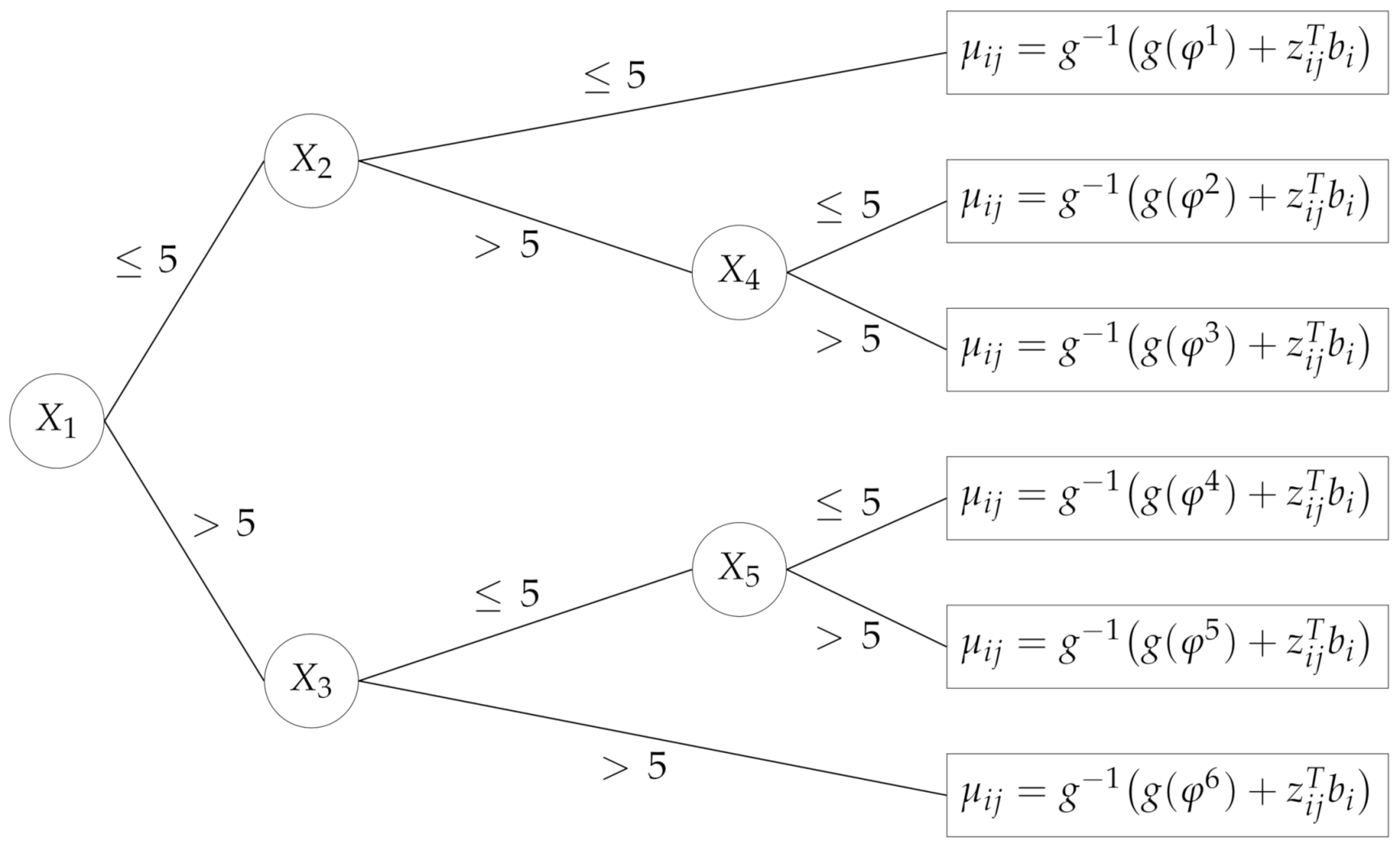
Let us define the fixed-effect structure. Eight random variables $X_1,\dots ,X_8$, independent and uniformly distributed in the interval $[0,10]$, were generated. While all of them were being used as predictors, only five of them were actually used to generate ${\mu }_{ij}$, based on the tree rule summarised in Figure 1. Each observation was classified into one of the six terminal nodes according to the values $x_{ij1},\dots ,x_{ij5}$. Within each leaf, values ${\phi }^1,\dots ,{\phi }^6$ denote the probabilities of success when the random effects $b_i$ are equal to zero:

• Leaf 1: if $x_{1ij}\le 5\wedge x_{2ij}\le 5$ then ${\mu }_{ij}=g^{-1}\left(g\left({\phi }^1\right)+z_{ij}^T{b}_i\right)$;
• Leaf 2: if $x_{1ij}\le 5\wedge x_{2ij}>5\wedge x_{4ij}\le 5$ then ${\mu }_{ij}=g^{-1}\left(g\left({\phi }^2\right)+z_{ij}^T{b}_i\right)$;
• Leaf 3: if $x_{1ij}\le 5\wedge x_{2ij}>5\wedge x_{4ij}>5$ then ${\mu }_{ij}=g^{-1}\left(g\left({\phi }^3\right)+z_{ij}^T{b}_i\right)$;
• Leaf 4: if $x_{1ij}>5\wedge x_{3ij}\le 5\wedge x_{5ij}\le 5$ then ${\mu }_{ij}=g^{-1}\left(g\left({\phi }^4\right)+z_{ij}^T{b}_i\right)$;
• Leaf 5: if $x_{1ij}>5\wedge x_{3ij}>5\wedge x_{5ij}>5$ then ${\mu }_{ij}=g^{-1}\left(g\left({\phi }^5\right)+z_{ij}^T{b}_i\right)$;
• Leaf 6: if $x_{1ij}>5\wedge x_{3ij}>5$ then ${\mu }_{ij}=g^{-1}\left(g\left({\phi }^6\right)+z_{ij}^T{b}_i\right)$;

where $g\left(·\right)$ is the logit link function. Two different possibilities were specified for the fixed effects: in the large fixed-effects specification, the standard deviation of the typical probabilities across the leaves was higher than in the small one (0.37 versus 0.24).

The random component $b_i\sim N(0,\Psi )$ was generated according to three different possibilities:

• No random effects: $\Psi =0$;
• Random intercept: $z_{ij}=1\forall i,\forall j$ and $\Psi ={\psi }_{11}$;
• Random intercept and slope, which add a linear random effect for the fixed-effect covariate $X_1$, uncorrelated from the random effect on the intercept. That is, $z_{ij}={\left[1x_{1ij}\right]}^T\forall i,\forall j$ and $\Psi =\left[\begin{array}{cc}{\psi }_{11}& 0\\ 0& {\psi }_{22}\end{array}\right]$.

Within each fixed-effects scenario with random effects, we considered two specifications (low and high) for the covariance matrix $\Psi$ to account for different levels of magnitude of the between-group variability.

Simulation Results

We ran eight different models for each one of the 10 DGPs:

• A standard binary classification tree model (Std);
• A random intercept GMET model (RI);
• A random intercept and slope GMET model (RIS);
• A parametric mixed-effects logistic regression model (MElog) that used the true model leaves’ indicators as fixed covariates and the true random effect structure;
• A parametric mixed-effects logistic regression model (GLMM) that used $(x_1,\dots ,x_8)$ as fixed covariates and the true random effect structure;
• The GLMERT algorithm proposed in [11] considering $(x_1,\dots ,x_8)$ as fixed covariates and the true random effect structure;
• The GMERT algorithm proposed in [10] considering $(x_1,\dots ,x_8)$ as fixed covariates and the true random effect structure;
• The BiMM algorithm proposed in [12] considering $(x_1,\dots ,x_8)$ as fixed covariates and a random intercept4.

As noted in Hajjem et al. [9], the MElog model could not be a real competitor of any other model. Indeed, it is not possible in practice to specify this parametric structure without knowing the underlying data generating process. This model only serves as a reference for the performances of the other models. In tree-based models, we fixed to 10 the maximum depth parameter and to 20 the minimum number of observations necessary to attempt a split5. After fitting each model on the training set, we could compute the corresponding predicted probability ${\widehat{\mu }}_{ij}$ and the predicted class ${\widehat{y}}_{ij}$ of observation j in group i in the test dataset. While the former was directly estimated by the algorithm, the latter depended on the threshold value ${\mu }_k^{*}$ used to classify subjects in the test set: ${\widehat{\mu }}_{ij}\ge {\mu }_k^{*}\Rightarrow {\widehat{y}}_{ij}=1$ where $(i,j)\in \mathrm{test}$. There were at most K distinct fitted values ${\mu }_k$, with $K\le I\left|T\right|$. We used each of them to classify observations in the training set and we fixed the threshold ${\mu }_k^{*}$ as the one that yields the closest proportion of class 1 to the actual proportion of class 1 in the training set.

We measured the predictive performance by:

• The predictive mean absolute deviation

  $$\mathrm{PMAD}=\frac{1}{N_{t}est}\sum _{i=1}^I\sum _{j=1}^{n_i^{t}est}\left|{\mu }_{ij}-{\widehat{\mu }}_{ij}\right|$$
• The predictive misclassification rate (PMCR)

  $$\mathrm{PMCR}=\frac{1}{N_{t}est}\sum _{i=1}^I\sum _{j=1}^{n_i^{t}est}\left|y_{ij}-{\widehat{y}}_{ij}\right|.$$

The mean, median, standard deviation, minimum and maximum of the PMAD and the PMCR over 100 runs were calculated and are reported in

Table 2. Results of the 100 simulation runs in terms of predictive probability mean absolute deviation (PMAD) and predictive misclassification rate (PMCR) for the eight models for the 10 DGPs. DGPs for which the performance gap between MElog and GMET was the largest or the smallest are marked in bold.

DGP	Random Effect	Fixed Effect	Fitted Model	PMAD(%)					PMCR(%)
				Mean	Median	SD	Min	Max	Mean	Median	SD	Min	Max
1	NO RANDOM EFFECT	Large	Std	5.01	4.59	1.93	2.10	9.83	16.76	16.46	1.55	14.64	21.68
			RI	20.89	20.98	2.34	13.43	24.92	31.52	31.50	2.54	24.16	36.68
			RIS	20.91	21.02	2.22	13.18	25.21	31.12	31.30	2.14	23.20	35.96
			MElog	3.36	3.28	1.15	1.30	5.84	17.55	16.08	3.30	13.76	24.64
			GLMM	21.61	21.58	0.78	19.88	23.14	30.10	30.20	0.92	27.52	31.56
			GLMERT	5.73	5.43	2.17	2.37	11.02	19.38	18.50	3.01	14.76	25.04
			GMERT	4.85	4.33	1.84	1.96	9.45	17.80	17.70	1.73	15.12	21.64
			BiMM	21.54	23.09	3.23	16.63	26.21	30.49	30.52	1.33	25.16	33.44
2		Small	Std	9.97	10.22	3.29	4.49	17.62	32.24	32.72	2.39	28.00	38.64
			RI	13.66	13.58	1.82	10.48	18.13	37.24	37.42	2.11	32.68	41.48
			RIS	13.89	13.68	1.83	10.98	18.31	37.36	37.40	1.92	33.52	41.96
			MElog	4.07	4.02	1.35	1.42	7.74	28.84	28.80	1.79	25.96	34.48
			GLMM	15.43	15.35	0.54	14.09	16.67	37.44	37.48	1.20	34.72	40.08
			GLMERT	10.10	10.01	3.01	6.59	15.40	34.14	34.08	2.72	29.00	38.80
			GMERT	10.03	10.08	2.87	6.42	14.54	33.31	32.86	4.23	28.80	42.64
			BiMM	12.60	13.50	1.77	9.65	15.10	34.60	34.52	1.79	31.12	38.56
3	Low	Large	Std	23.39	22.95	2.93	18.01	29.90	29.26	28.62	3.31	23.40	36.36
			RI	18.28	18.12	1.57	13.81	22.98	26.98	26.96	2.05	21.92	32.20
			RIS	18.46	18.39	1.59	14.01	22.79	27.09	26.96	2.03	22.08	32.24
			MElog	8.69	8.61	0.75	7.60	10.85	19.65	19.46	1.12	17.72	23.24
			GLMM	18.62	18.67	1.05	16.74	20.96	26.69	26.70	1.56	23.80	30.40
			GLMERT	11.95	11.94	2.54	7.83	17.59	21.93	21.40	3.18	18.00	30.76
			GMERT	23.70	22.87	3.02	19.43	28.76	29.05	28.52	3.99	23.72	38.00
			BiMM	27.68	27.93	2.03	22.61	31.17	35.52	35.28	2.14	30.72	40.24
4	High		Std	31.70	31.94	2.58	26.22	36.78	36.23	36.20	3.12	30.32	44.16
			RI	15.38	15.46	1.51	11.96	18.57	20.68	20.68	1.97	16.64	25.76
			RIS	15.44	15.67	1.44	12.03	18.53	20.78	20.80	1.97	16.68	25.92
			MElog	8.21	8.06	0.95	6.21	11.01	15.78	15.70	1.50	12.56	20.12
			GLMM	15.40	15.36	1.29	12.01	17.76	20.66	20.60	1.93	16.40	24.88
			GLMERT	10.65	10.50	1.32	8.40	12.76	18.08	17.92	1.14	16.48	19.96
			GMERT	29.67	29.39	2.80	25.92	35.46	32.68	31.36	4.25	27.84	42.76
	INTERCEPT		BiMM	32.69	32.48	2.00	28.93	35.80	38.39	38.52	2.60	31.12	43.84
5	Low	Small	Std	15.79	15.87	2.39	10.13	22.90	34.30	34.92	2.35	29.00	38.56
			RI	15.68	15.77	1.68	13.11	19.26	35.74	35.74	2.30	31.24	43.12
			RIS	15.87	15.89	1.61	13.14	19.18	35.74	35.64	2.06	31.72	42.72
			MElog	8.55	8.61	0.92	6.45	10.73	28.80	28.66	0.99	25.84	30.96
			GLMM	16.48	16.35	0.59	15.13	18.23	36.47	36.60	1.21	33.52	39.32
			GLMERT	13.28	13.37	1.12	11.62	15.21	33.35	32.86	2.35	30.64	39.84
			GMERT	14.63	15.14	1.38	11.91	16.65	33.90	32.74	3.16	31.12	42.20
			BiMM	16.48	16.38	2.01	12.89	20.41	36.21	35.56	1.87	33.40	41.40
6	High		Std	27.98	28.16	2.33	23.28	32.46	41.23	40.88	3.09	35.92	50.44
			RI	14.02	13.99	1.62	10.01	17.45	25.87	26.14	2.41	20.64	30.56
			RIS	14.13	14.17	1.66	10.08	17.29	25.89	26.00	2.37	20.68	30.52
			MElog	9.41	9.43	1.10	7.24	11.79	22.85	23.22	1.66	20.00	26.36
			GLMM	14.24	14.13	1.05	11.95	16.82	25.98	25.88	2.02	22.32	30.96
			GLMERT	13.05	12.49	2.85	9.54	19.24	25.98	25.48	2.71	22.40	31.28
			GMERT	26.61	27.13	2.44	21.32	30.06	32.79	32.90	2.65	27.76	37.96
			BiMM	27.27	27.60	2.15	23.61	30.45	40.83	40.72	2.80	33.32	46.76
7	Low	Large	Std	22.16	22.47	2.28	17.32	27.38	28.08	28.60	2.69	22.32	34.20
			RI	20.08	20.05	1.38	15.17	22.67	28.52	28.44	1.51	23.48	30.80
			RIS	19.64	19.67	1.29	16.00	22.64	28.34	28.14	1.44	24.20	30.68
			MElog	9.95	10.00	0.95	8.12	12.78	20.09	20.00	0.90	18.44	22.20
			GLMM	19.93	19.93	1.10	17.59	21.92	27.93	27.88	1.42	25.04	31.00
			GLMERT	12.10	11.80	1.57	10.30	15.72	21.76	21.92	1.04	20.24	24.32
			GMERT	14.71	14.89	1.34	12.55	16.85	23.05	22.62	1.35	21.68	25.76
			BiMM	26.39	26.53	1.50	22.72	28.52	35.04	35.40	1.80	31.00	38.52
8	High		Std	32.57	32.42	2.85	26.92	38.29	37.46	36.82	4.12	30.36	49.68
			RI	17.29	17.38	1.53	13.56	20.87	21.66	21.42	2.19	17.68	25.64
			RIS	15.82	15.89	1.56	11.80	18.42	20.72	20.58	2.18	17.08	24.72
			MElog	9.50	9.48	0.82	7.72	10.97	16.09	16.16	1.40	12.24	19.00
			GLMM	15.87	15.75	1.34	13.55	18.82	20.57	20.28	2.14	16.52	25.60
			GLMERT	13.08	13.38	1.62	10.15	15.57	18.92	19.54	1.64	16.08	20.76
			GMERT	17.63	17.38	1.34	16.04	20.71	21.33	21.66	2.05	18.08	25.04
	INTERCEPT & SLOPE		BiMM	33.62	33.40	1.61	30.70	37.02	39.41	39.48	2.71	33.48	44.80
9	Low	Small	Std	16.55	16.78	2.25	11.52	20.62	35.13	35.12	2.43	29.76	39.52
			RI	15.94	15.62	1.43	12.37	18.89	36.37	36.18	2.11	31.92	41.04
			RIS	15.83	15.55	1.47	12.19	18.91	36.17	36.28	1.88	31.92	41.08
			MElog	9.04	8.84	0.87	7.35	11.39	29.03	29.06	0.97	26.72	31.20
			GLMM	16.81	16.66	0.76	15.11	18.64	36.71	36.72	1.36	34.00	40.20
			GLMERT	13.45	13.64	2.06	10.04	17.46	32.92	32.72	2.93	28.36	38.64
			GMERT	13.05	13.04	1.89	10.38	16.16	32.81	33.04	2.59	28.68	37.12
			BiMM	16.37	15.82	1.72	13.96	19.86	36.47	35.96	2.20	32.64	41.48
10	High		Std	26.95	26.57	2.26	22.70	31.94	40.45	39.98	3.19	33.52	47.76
			RI	15.76	15.90	1.40	12.71	18.94	27.97	27.90	2.19	22.52	32.76
			RIS	15.28	15.14	1.39	12.73	18.65	27.61	27.56	2.23	22.72	31.56
			MElog	10.80	10.76	1.10	7.86	13.74	24.25	24.24	1.75	20.48	28.16
			GLMM	15.45	15.43	1.00	13.18	17.42	27.65	27.88	2.08	23.12	31.96
			GLMERT	15.77	16.32	1.79	13.08	18.61	28.03	28.48	2.05	23.92	30.80
			GMERT	17.77	18.44	1.79	14.72	20.49	29.83	29.80	2.17	25.56	33.52
			BiMM	25.41	24.92	2.14	21.90	29.44	39.33	38.92	2.73	34.56	45.36

.

We observed that when there was no random effect (DGPs 1 and 2), the standard classification tree algorithm performed better than the mixed-effects models, especially when the fixed effect was large. Nonetheless, in the latter scenario, the performances of GLMERT and GMERT were very close to Std ones, proving to be robust even in absence of a true random effect. However, when random effects were present (DGPs 3 to 10), mixed-effects classification trees performed better than the standard classification tree in terms of average PMAD and PMCR. BiMM is the only mixed-effects tree algorithm whose performance was very close to $Std$ ones, for all DGPs6. When the DGP included only a random intercept, GLMERT had the best predictive performance, and was directly followed by RI. When the true random effect structure included both random intercept and random slope, GMERT, GLMERT and RIS performances were very close. There was a slightly better performance by GLMERT when the fixed effect was large and of RIS when the fixed effect was small. The highest improvement in PMAD using a mixed tree model was observed when both the fixed and the random effects were large. The lowest improvement was observed when both the fixed and the random effects were small. Analogous statements can be made about PMCR. In addition, GMET performed better than standard trees even when we fit a mixed tree whose random component was over-specified (as in DGPs 3–6, Std vs RIS) or under-specified (as in DGPs 7–10, Std vs RI) in relation to the true data generating process.

Next, we compare the performance of the GMET approach to the results of the MElog reference model. If the DGP did not include random effect, the difference between PMAD and PMCR was higher when the fixed effect was large (DGP 1). When the random effect was large and the fixed effect was small (DGPs 6 and 10), the GMET model performed similiarly to the MElog model. In terms of PMAD, the differences were 4.61% and 4.48% for DGPs 6 and 10, respectively; in terms of PMCR, they were 3.02% and 3.36%, respectively. The difference in predictive accuracy between the two models reached its maximum when the random effect was small and the fixed effect was large (DGPs 3 and 7). In terms of PMAD, the differences were 9.59% and 9.69% in DGPs 3 and 7, respectively; in terms of PMCR, they were 7.33% and 8.25%, respectively.

With respect to the other existing tree-based mixed-effects models, the fact that the GMET algorithm is not iterative makes it less performant when fixed and when its random effects are small and easier to be confused; and its performs better when they are large and easier to be disentangled. Moreover, its step through a glm makes it perform worse when the DGP includes only a large (in this case, nonlinear) fixed effect, but makes it competitive with the other existing methods when data have an important random-effects structure.

In order to investigate the performance and to deepen the comparison across methods under different settings, we report, in Appendix B, additional simulations and results: we provide more details about the model’s predictive quality in this simulation, e.g., the recovery of the right tree structure or the identification of the right number of leaves. We ran new simulations for different DGPs (linear and non-linear fixed-effects) and for a different response variable in the exponential family, i.e., Poisson. Results show that GMET on average outperformed all other tree-based methods when data had a linear structure, for both a binary and a Poisson response variable.

4. Case Study: Application of the Mixed-Effects Tree Algorithm to Education PoliMi Data

In this section, we describe the PoliMi dataset. We applied the generalised mixed-effects tree algorithm to these data. Using a GMET model, we could identify discriminating fixed-effects covariates and estimate the degree programme’s effect on the predicted success probability. In addition, we also analysed the accuracy of this model for predicting dropout.

The PoliMi dataset consists of 18,612 records in Bachelor of Science (BSc) students that began between A.Y. 2010/2011 and 2013/2014. Students are nested within $I=19$ degree programmes.

Table 3. Number of students enrolled in the 19 PoliMi degree programmes between A.Y. 2010/2011 and 2013/2014.

Degree Program	Number of Students
Aerospace Engineering	1127
Automation Engineering	538
Biomedical Engineering	1456
Building Engineering	671
Chemical Engineering	715
Civil and Environmental Engineering	405
Civil Engineering	855
Electrical Engineering	575
Electronic Engineering	567
Energy Engineering	1485
Engineering of Computing Systems	2173
Environmental and Land Planning Engineering	590
Industrial Production Engineering	288
Management Engineering	2750
Materials and Nanotechnology Engineering	637
Mathematical Engineering	575
Mechanical Engineering	2364
Physics Engineering	469
Telecommunications Engineering	372

reports the list of the 19 degree programmes and the number of students enrolled in each degree program. A descriptive analysis showed that a high percentage of students leave the Politecnico before obtaining a degree. In particular, the sample shows a $37.11\%$ dropout rate. Therefore, our goal was to find out which student-level indicators could discriminate between two different profiles: dropout and graduate students.

We assumed a binary GMET model (3) where student j was nested within degree programme i. The response variable Y was the status, a two-level factor we coded as a binary variable:

• status$=1$ for studies definitely completed with graduation;
• status$=0$ for studies definitely concluded with dropping out.

We would like to make predictions at the very early stages of students’ academic careers. Thus, we chose as predictors five variables available at the time of enrolment and three more variables collected just after the first semester of study. The list and explanation of student-level variables to be included as covariates is reported in

Table 4. A list and explanations of variables at the student level which were included as covariates in the GMET model.

Variable	Description	Type of Variable
Sex	gender	factor (2 levels: M, F)
Nationality	nationality	factor (Italian, foreigner)
PreviousStudies	high school studies	factor (Liceo Scientifico,
		Istituto Tecnico, Other)
AdmissionScore	PoliMi admission test result	real number
AccessToStudiesAge	age at the beginning of the	natural number
	BSc studies at PoliMi
WeightedAvgEval1.1	weighted average of the evaluations	real number
	during the first semester of the first year
AvgAttempts1.1	average number of attempts to be	real number
	evaluated on subjects during
	the first semester of the first year
	(passed and failed exams)
TotalCredits1.1	number of ECTS credits obtained	natural number
	by the student during the first
	semester of the first year

. In addition, we chose as the grouping variable the degree programme at the time of enrolment (factor DegreeProgramme) which has 19 levels. The influence of the grouping factor on the predictor was modelled through a group-level intercept $b_i$. We randomly split the dataset into training and test subsets, with a ratio of 80% for training and 20% for evaluation. Thus, the training subset included 14,890 students and the test subset had 3722.

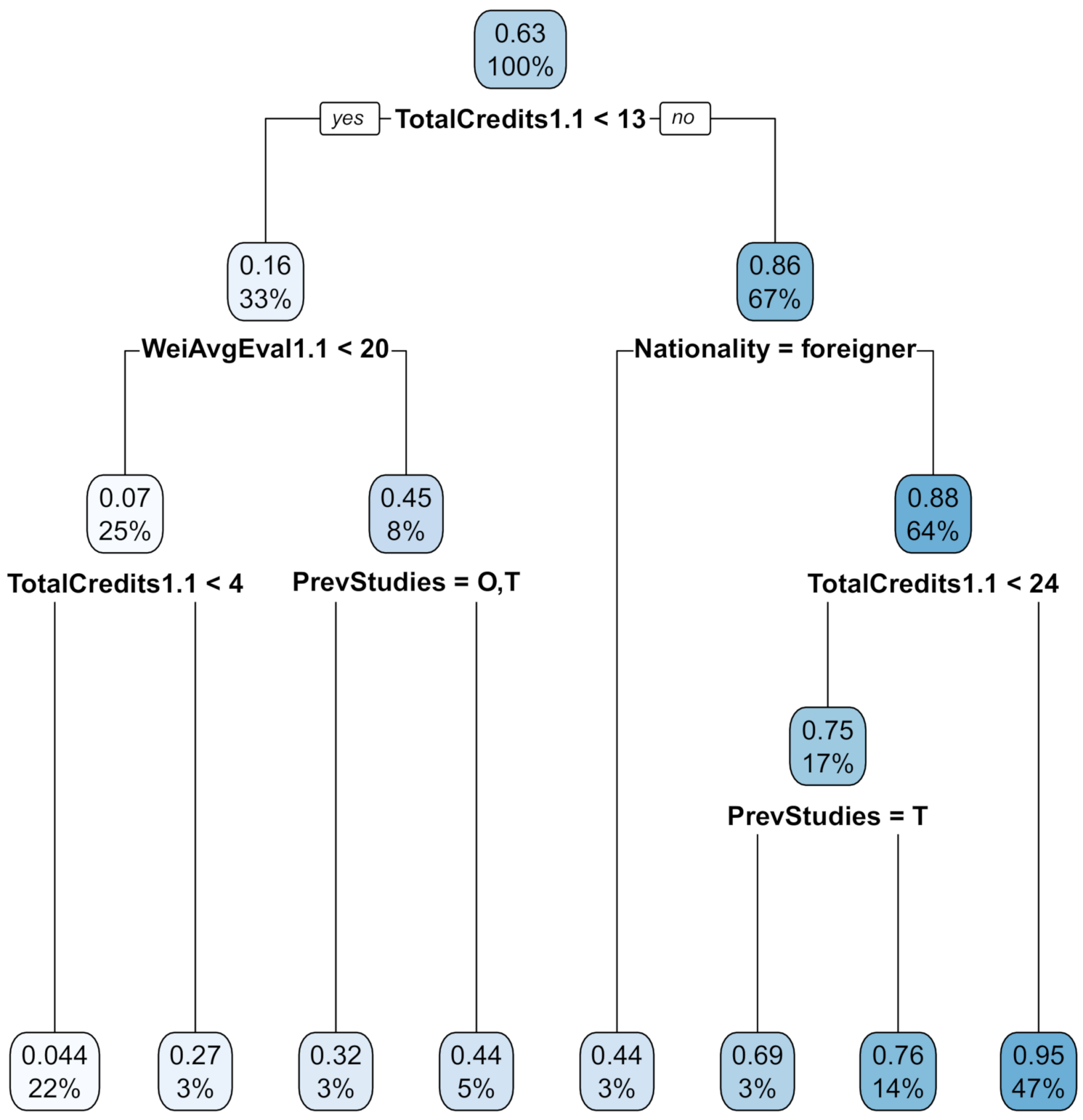
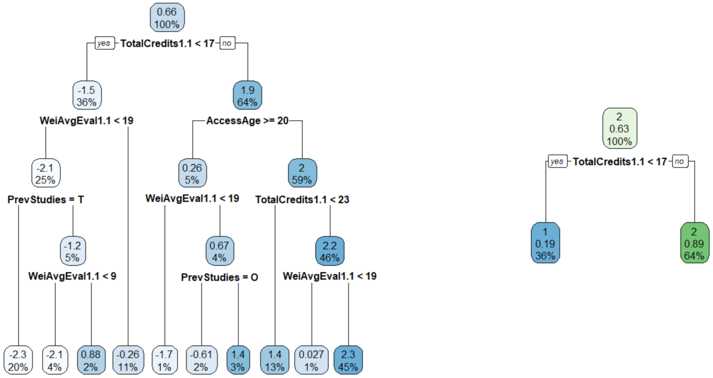
While growing the tree, we fixed to 10 the maximum depth parameter and to 20 the minimum number of observations necessary to attempt a split. Figure 2 shows the estimated mixed-effects tree for the probability of graduation. Every internal node had a corresponding condition that split it into two children: if the condition was true, observations were sent down the tree through the left child; if the condition was false, through the right child. In addition, all nodes reported two values: the estimated probability of graduation and the percentage of observations in the node over the total training set. We remind the reader that variable PreviousStudies has been coded as a three-level factor with levels S (Liceo Scientifico), T (Istituto Tecnico) and O (other high school studies). The number of ECTS obtained in the first semester of the first year was used as the first split: students who obtained less than 13 ECTS were associated with lower success probability (0.16 versus 0.86). Then, students were further classified using other explanatory variables: we can see that Italian students who obtained more than 24 ECTS had the highest predicted success probability (0.95). Other variables actually used to split smaller internal nodes were Nationality and PreviousStudies: in these nodes, students who attended Istituto Tecnico and foreign students had lower predicted success than the others. Through this model, it was possible to find out significant interactions among the covariates: for example, variable Nationality was used to split the group of students that obtained at least 13 ECTS, but this same variable did not appear in the complementary branch of the tree. Finally, covariates Sex, AdmissionScore and AvgAttempts1.1 were not compared in the trees, so they do not appear to have strong influences on how one’s studies end.

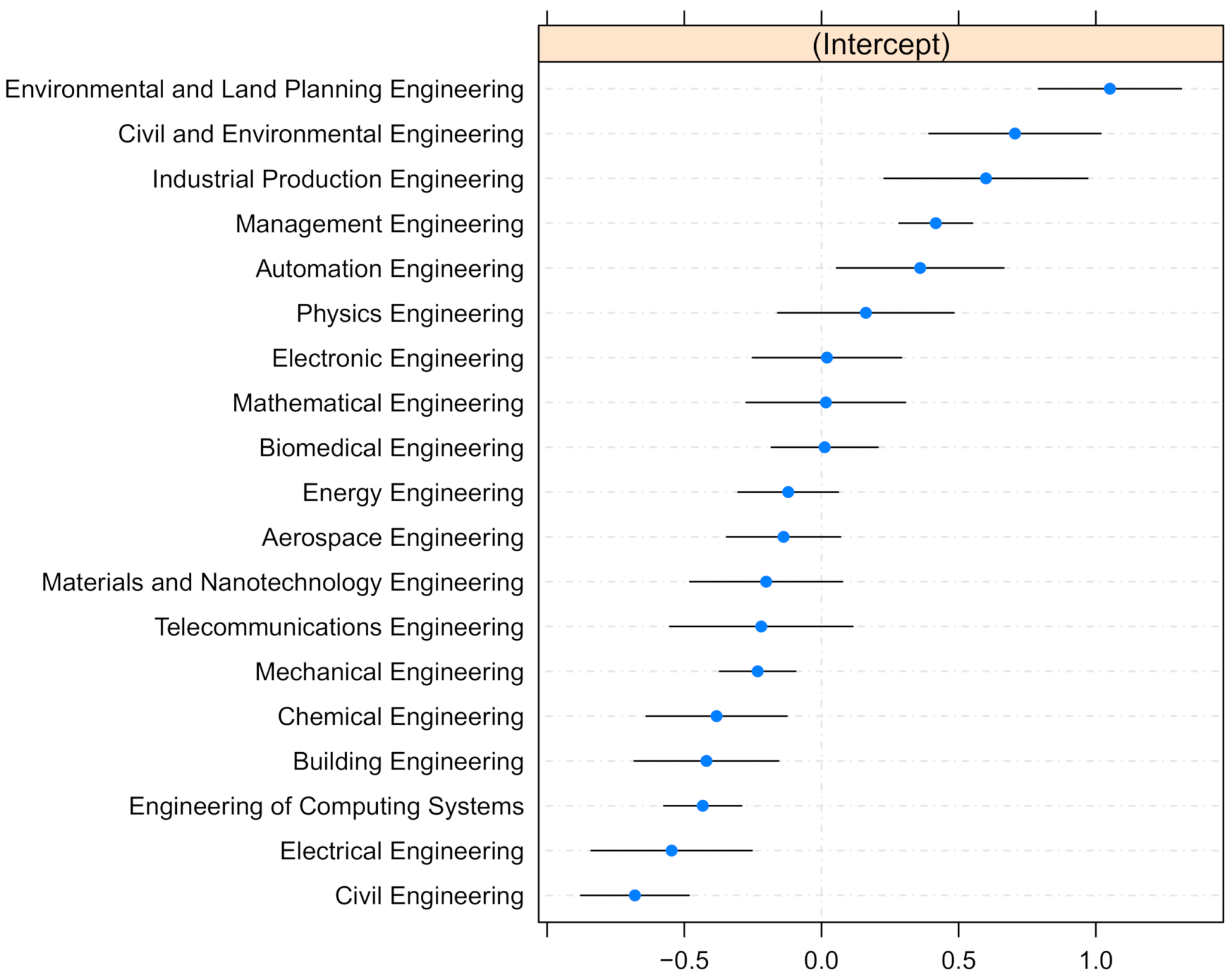
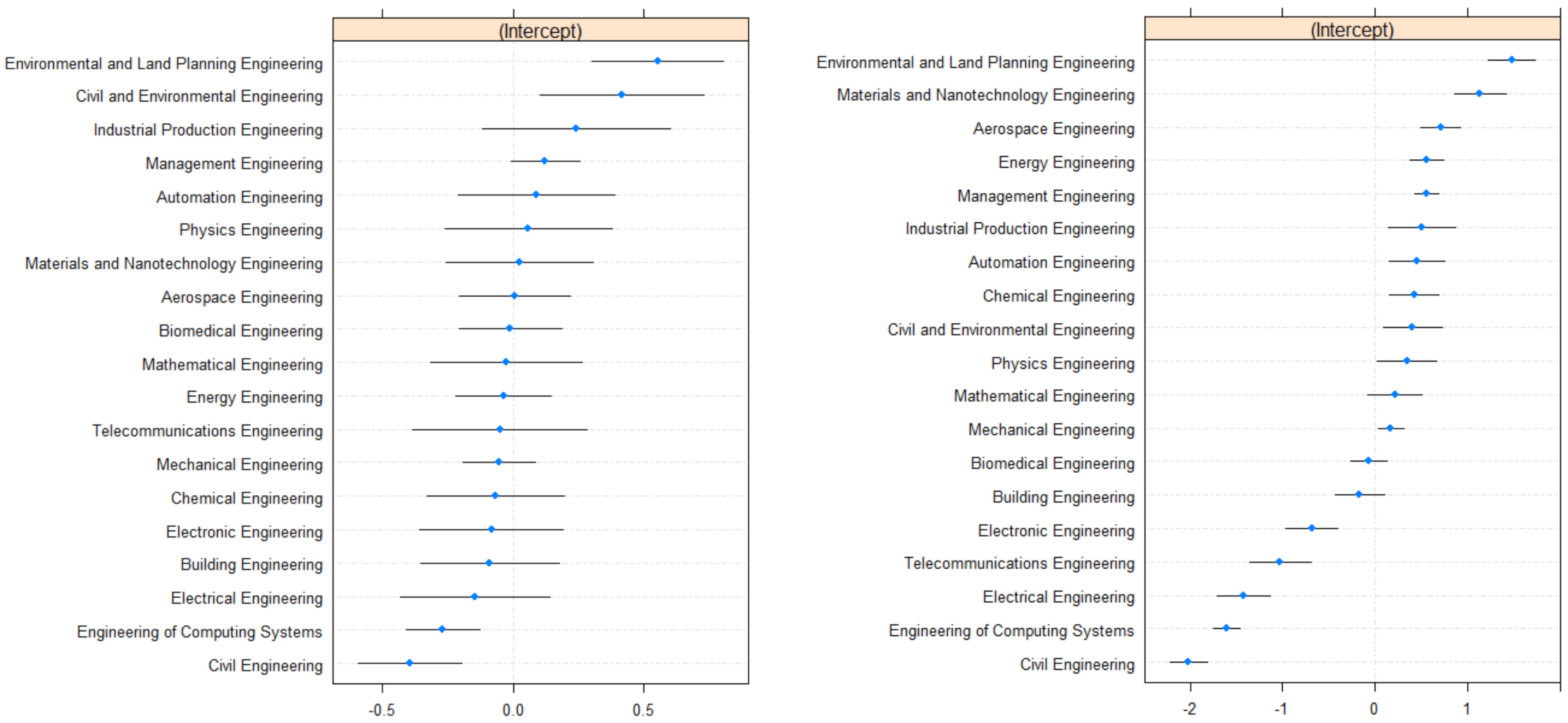
Using the tree structure in Figure 2, we could get population-level predictions for new observations that did not include the effect of the programme. However, if we also specified the level of the random effect covariate, our model was able to adjust this prediction to account for the effect and make a group-specific prediction. Indeed, we extracted coefficients ${\widehat{b}}_i$ from the full estimated mixed model (3) and provide different predictions for different programmes within each leaf of the tree structure. Figure 3 shows the ranking of the 19 estimated random-effects intercepts, one for each degree program. Light blue points correspond to the point estimates ${\widehat{b}}_i$, for $i=1,\dots ,19$, and the horizontal black lines represent the $95\%$ confidence intervals of the estimates. When the $95\%$ confidence interval does not overlap with 0 (identified by the dashed vertical line), we have evidence to assert that the degree program’s effect was significantly different from zero, i.e., from the average. For many groups, the 95% confidence interval does not overlap with the vertical line at zero, underlining substantial differences between the groups. If we use this model to estimate the probability of graduation, many degree programs will give results significantly different from the average. In particular, degree programs whose confidence intervals are entirely higher (lower) than zero are associated with higher (lower) dropout likelihood with respect to the average, all else being equal. After fixing all other covariates, Environmental and Land Planning Engineering and Civil and Environmental Engineering had large positive effects on the intercept: one student from one of those programmes improves the log odds by $1.051$ or $0.705$, respectively. On the contrary, studying either Civil Engineering or Electrical Engineering penalises the log odds by $0.680$ and $0.546$ respectively.

Since we were using a multilevel model, we were able to account for the interdependence of observations by partitioning the total variance into different components due to the clustered data structure in model (3). The variance partition coefficient (VPC) is a possible measure of intraclass correlation: it is equal to the percentage of variation that is found at the higher level of hierarchy over the total variance [39]. The idea of VPC was extended using the latent variable approach, to define a method to partition the total variance in the case of a binary response and the group-specific intercept for the random-effects structure [40]. In this case, the variance partition coefficient was constant across all individuals, and it can be estimated as:

$$\begin{array}{c}\hfill \mathrm{VPC}=\frac{\widehat{\psi }}{\widehat{\psi }+{\sigma }_{lat}^2}=\frac{0.2988}{0.2988+{\pi }^2/3}=0.0612\end{array}$$

where $\widehat{\psi }$ is the estimated variance of the random intercept and ${\sigma }_{lat}^2$ is the residual variability that can be explained by neither fixed effects, nor the group features that are represented by the random intercept. In this case, it is equal to the variance of the standard logistic distribution. This VPC value means that $6.12\%$ of variation in the response is attributable to the classification by degree type. This value underlines the need to use a mixed model.

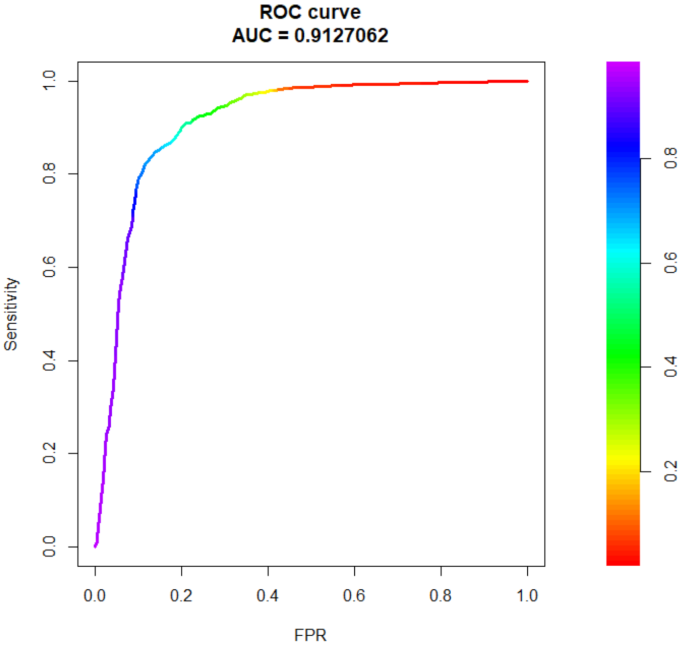
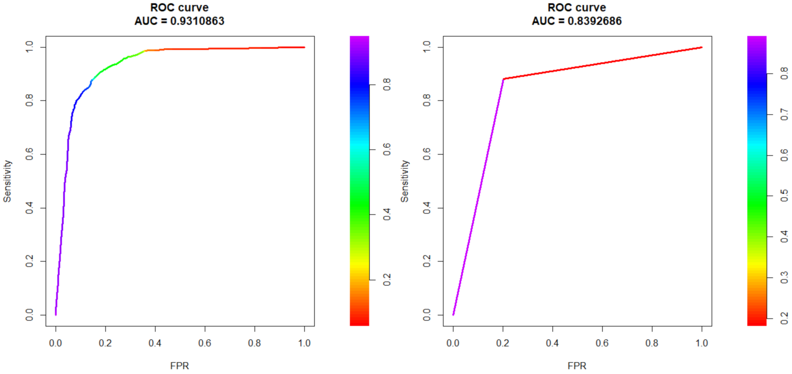
We can now evaluate the performance of the model and its predictive quality using the area under the ROC curve (AUC) and other performance indexes: accuracy, sensitivity and specificity. For each test observation, we were given a full set of covariates; therefore, we were able to compute an estimate $\widehat{p}$ of the probability of successfully concluding a BSc and getting a degree. We used this estimate to define a binary classifier based on model (3): we chose $p_0=0.6$ as the optimal cutoff value through ROC curve analysis, as shown in Figure 4. For 20 iterations, we randomly split the observations into training and test sets. We fit a GMET model with the training set, and we classified test observations using the optimal threshold value. Finally, we computed the average accuracy, sensitivity and specificity values and their standard deviations, which are reported in

Table 5. Performance indexes of the classifier based on the mixed-effects tree of model (3).

Index	Mean	Std Deviation
Accuracy	0.860	0.006
Sensitivity	0.816	0.012
Specificity	0.886	0.008

. High values of accuracy, sensitivity and specificity indicate a good model. The model’s performance was robust, as highlighted by the low standard deviations of the mean performance indexes and the high AUC, equal to $0.9127$ (Figure 4). In addition,

Table 6. Performance indexes of the classifier based on the mixed-effects tree of model (3), computed for each degree program.

Degree Program	Accuracy Mean (sd)	Sensitivity Mean (sd)	Specificity Mean (sd)
Aerospace Engineering	$0.880$ ($0.028$)	$0.845$ ($0.038$)	$0.897$ ($0.034$)
Automation Engineering	$0.880$ ($0.053$)	$0.798$ ($0.098$)	$0.925$ ($0.045$)
Biomedical Engineering	$0.894$ ($0.019$)	$0.860$ ($0.042$)	$0.912$ ($0.024$)
Building Engineering	$0.856$ ($0.042$)	$0.860$ ($0.080$)	$0.852$ ($0.050$)
Chemical Engineering	$0.877$ ($0.036$)	$0.889$ ($0.056$)	$0.873$ ($0.049$)
Civil and Environmental Engineering	$0.879$ ($0.038$)	$0.841$ ($0.081$)	$0.907$ ($0.052$)
Civil Engineering	$0.718$ ($0.041$)	$0.650$ ($0.044$)	$0.837$ ($0.060$)
Electrical Engineering	$0.849$ ($0.040$)	$0.840$ ($0.056$)	$0.867$ ($0.058$)
Electronic Engineering	$0.854$ ($0.037$)	$0.806$ ($0.078$)	$0.886$ ($0.053$)
Energy Engineering	$0.898$ ($0.023$)	$0.884$ ($0.059$)	$0.903$ ($0.022$)
Engineering of Computing Systems	$0.823$ ($0.022$)	$0.846$ ($0.029$)	$0.805$ ($0.030$)
Environmental and Land Planning Engineering	$0.851$ ($0.034$)	$0.782$ ($0.100$)	$0.878$ ($0.052$)
Industrial Production Engineering	$0.822$ ($0.091$)	$0.692$ ($0.164$)	$0.916$ ($0.068$)
Management Engineering	$0.873$ ($0.014$)	$0.765$ ($0.040$)	$0.931$ ($0.015$)
Materials and Nanotechnology Engineering	$0.907$ ($0.034$)	$0.867$ ($0.088$)	$0.918$ ($0.031$)
Mathematical Engineering	$0.893$ ($0.031$)	$0.851$ ($0.058$)	$0.908$ ($0.040$)
Mechanical Engineering	$0.863$ ($0.023$)	$0.841$ ($0.032$)	$0.875$ ($0.028$)
Physics Engineering	$0.902$ ($0.031$)	$0.852$ ($0.062$)	$0.930$ ($0.041$)
Telecommunications Engineering	$0.853$ ($0.058$)	$0.845$ ($0.087$)	$0.858$ ($0.061$)

reports the means and standard deviations of accuracy, sensitivity and specificity, computed separately for each degree program.

It is interesting to compare these average performance indexes against those obtained using different methods. Our approach had similar accuracy to a standard classification tree (0.878 versus 0.879), but its accuracy showed less variability across the iterations. For example, its standard deviation of accuracy was 0.5%; compare that to 2.8% for the classification tree. Since we were interested in the detection of dropout careers, we compared mean sensitivity using different models. Using mixed-effects trees, we attained higher sensitivity than using standard classification trees (0.835 versus 0.800). Thus, the choice of a mixed-effects model seemed appropriate: the degree programme is a meaningful covariate for the prediction of status. The mixed-effects tree was slightly less sensitive than a classifier built through a GLMM (0.835 versus 0.850), suggesting that a tree-like structure for fixed effects might not be as suitable as the GLMM one. However, it has other advantages, such as offering an easily interpretable model that could be graphically displayed and understood. Overall, the good performance of GMET in this application was due to two reasons. The first is that the variability at the highest level of grouping, i.e., degree programs, was not negligible, and therefore, taking it into account improved the predictive performance of the models. The second is that the good performance of the GLMM suggests that the association between the most important covariate, i.e., TotaleCredits1.1 (the most relevant variable in the tree of Figure 2), and the response can be well approximated by a linear function. Therefore, ${\widehat{\mu }}_{ij}$, estimated at step 2 of the GMET algorithm and used as the input for the tree built at step 3, was very precise and representative of the real dynamics, helping the GMET algorithm to fit the data well.

Appendix A reports the results of the application of GMERT and BiMM algorithms to the PoliMi case study and a comparison with GMET results presented in this section.

5. Conclusions

We proposed a multilevel tree-based model for a non-Gaussian response (GMET algorithm), showed a simulation study and applied the GMET algorithm to the PoliMi careers dataset as a tool to find student-level variables to discriminate between two different student profiles (graduate and dropout) and to estimate the degree programme’s effect on the predicted success probability.

The GMET model can deal with a grouped data structure, while providing easily interpretable models that can outline complex interactions among the input variables. In the simulation study, the performance of the proposed mixed-effects tree method was a marked improvement over the CART model when the data generating process (DGP) included random effects, even if they were of small magnitude. In addition, the performance of the GMET model was similar to that of the benchmark logistic model that was fitted assuming the whole specification of the DGP. GMET’s performance was comparable to that of other existing tree-based mixed-effects models, outperforming them when data had a linear structure, and it had a clear advantage in convergence time. Although our study focused on the binary response case, the mixed-effects tree approach could be extended to other types of response variables. Using a suitable link function, we could study if the method is appropriate to model different outcomes, such as count data or a multinomial factor response. Overall, the main advantages of the GMET algorithm are its flexibility and interpretability [41]. By relaxing the linear assumption of the fixed-effects part, the method could model more complex functional forms, easily treating potential interactions among covariates. This complexity is then summarised in a tree structure, which is easy to interpret and communicate. At the same time, when data present a hierarchy, the method is able to take into account the dependence structure within observations and to model it. In the educational data mining context, this aspect is essential in order to better understand students and the settings in which they learn. On the other hand, GMET, as CARTs, suffers from high variance. This means that if we split the training data into two parts at random, and fit a decision tree to both halves, the results could be quite different. Ensemble methods which use a mixed-effects tree as a base learner together with a random forest approach may be developed.

In our case study, the effectiveness of the GMET model in dropout prediction was comparable to the effectiveness of more established classification methods. A GMET model with high accuracy and sensitivity was obtained by considering information available at the time of the admission and the results of the first semester of studies. In addition, our work identifies a significant effect of the engineering programme on dropout probability. The estimated student success probability might be used as a tool to conduct policy experiments at the institutional level, aimed at identifying the best practices to help and retain at-risk students. In this setting, PoliMi started an experimental early intervening program that invites at-risk students (identified by the GMET algorithm) to attend dedicated tutorship to support them during the beginning of their studies at PoliMi.

In the context of the SPEET project, a future development could be the extension of our analysis to the other project partners in order to compare the programme effect at the country level. This would allow us to relate this effect to programme-level variables, and we could establish whether the same profiles of students at risk of dropout arise at country level. Moreover, in accordance with the validity and the potential of the GMET method when applied to modelling student dropout prediction, our future perspective goes in the direction of major applications in the learning analytics area. This method, when applied to educational data, can be a useful tool to support the definition of best practices and new tutoring programmes aimed at enhancing student performances and reducing student dropout. A worthwhile consideration is also the approach that teachers and students have with respect to its results. Indeed, this method is also valuable from the perspective of recommendation systems, since, if its results are interpreted and communicated in the right way, they can be used to drive students in their career choices.

References

- SPEETproject. SPEET, Proposal for Strategic Partnerships (Proposal Narrative). 2017. Available online: https://www.speet-project.com/the-project (accessed on 5 May 2020).
- Barbu, M.; Vilanova, R.; Lopez Vicario, J.; Pereira, M.J.; Alves, P.; Podpdora, M.; Ángel Prada, M.; Morán, A.; Torreburno, A.; Marin, S.; et al. Data mining tool for academic data exploitation: Literature review and first architecture proposal. In Projecto SPEET-Student Profile for Enhancing Engineering Tutoring; IEEE Access: Piscataway, NJ, USA, 2017. [Google Scholar]
- Romero, C.; Ventura, S. Educational data mining: A review of the state of the art. IEEE Trans. Syst. Man Cybern. Part C Appl. Rev. 2010, 40, 601–618. [Google Scholar] [CrossRef]
- Bock, R.D. Multilevel Analysis of Educational Data; Elsevier: London, UK, 2014. [Google Scholar]
- Goldstein, H. Multilevel Statistical Models; John Wiley & Sons: lWest Sussex, UK, 2011; Volume 922. [Google Scholar]
- Agresti, A. An Introduction to Categorical Data Analysis; Wiley: Hoboken, NJ, USA, 2018. [Google Scholar]
- Breiman, L.; Friedman, J.H.; Olshen, R.A.; Stone, C.J. Classification and Regression Trees, The Wadsworth Statistics and Probability Series; Wadsworth International Group: Belmont, CA, USA, 1984; p. 356. [Google Scholar]
- Sela, R.J.; Simonoff, J.S. RE-EM trees: A data mining approach for longitudinal and clustered data. Mach. Learn. 2012, 86, 169–207. [Google Scholar] [CrossRef] [Green Version]
- Hajjem, A.; Bellavance, F.; Larocque, D. Mixed effects regression trees for clustered data. Stat. Probab. Lett. 2011, 81, 451–459. [Google Scholar] [CrossRef]
- Hajjem, A.; Larocque, D.; Bellavance, F. Generalized mixed effects regression trees. Stat. Probab. Lett. 2017, 126, 114–118. [Google Scholar] [CrossRef]
- Fokkema, M.; Smits, N.; Zeileis, A.; Hothorn, T.; Kelderman, H. Detecting treatment-subgroup interactions in clustered data with generalized linear mixed-effects model trees. Behav. Res. Methods 2018, 50, 2016–2034. [Google Scholar] [CrossRef]
- Speiser, J.L.; Wolf, B.J.; Chung, D.; Karvellas, C.J.; Koch, D.G.; Durkalski, V.L. BiMM tree: A decision tree method for modeling clustered and longitudinal binary outcomes. In Communications in Statistics-Simulation and Computation; Taylor & Francis: Boca Raton, FL, USA, 2020; Volume 49, pp. 1–20. [Google Scholar]
- Zeileis, A.; Hothorn, T.; Hornik, K. Model-based recursive partitioning. J. Comput. Graph. Stat. 2008, 17, 492–514. [Google Scholar] [CrossRef] [Green Version]
- Cabrera, A.F.; Stampen, J.O.; Hansen, W.L. Exploring the effects of ability to pay on persistence in college. Rev. High. Educ. 1990, 13, 303–336. [Google Scholar] [CrossRef]
- John, E.P.S.; Paulsen, M.B.; Starkey, J.B. The nexus between college choice and persistence. Res. High. Educ. 1996, 37, 175–220. [Google Scholar] [CrossRef]
- Pascarella, E.T.; Terenzini, P.T. Predicting freshman persistence and voluntary dropout decisions from a theoretical model. J. High. Educ. 1980, 51, 60–75. [Google Scholar] [CrossRef]
- Spady, W.G. Dropouts from higher education: An interdisciplinary review and synthesis. Interchange 1970, 1, 64–85. [Google Scholar] [CrossRef]
- Tinto, V. Dropout from higher education: A theoretical synthesis of recent research. Rev. Educ. Res. 1975, 45, 89–125. [Google Scholar] [CrossRef]
- Korhonen, V.; Rautopuro, J. Identifying problematic study progression and “at-risk” students in higher education in Finland. Scand. J. Educ. Res. 2019, 63, 1056–1069. [Google Scholar] [CrossRef]
- Seidel, E.; Kutieleh, S. Using predictive analytics to target and improve first year student attrition. Aust. J. Educ. 2017, 61, 200–218. [Google Scholar] [CrossRef]
- Sothan, S. The determinants of academic performance: Evidence from a Cambodian university. Stud. High. Educ. 2019, 44, 2096–2111. [Google Scholar] [CrossRef]
- Saa, A.A.; Al-Emran, M.; Shaalan, K. Factors affecting students’ performance in higher education: A systematic review of predictive data mining techniques. Technol. Knowl. Learn. 2019, 24, 567–598. [Google Scholar]
- Wook, M.; Yusof, Z.M.; Zakree, M.; Nazri, A. Educational data mining acceptance among undergraduate students. Educ. Inf. Technol. 2017, 22, 1195. [Google Scholar] [CrossRef]
- Tampakas, V.; Livieris, I.E.; Pintelas, E.; Karacapilidis, N.; Pintelas, P. Prediction of students’ graduation time using a two-level classification algorithm. In Proceedings of the International Conference on Technology and Innovation in Learning, Teaching and Education, Thessaloniki, Greece, 20–22 June 2018; Springer: Berlin/Heidelberg, Germany, 2018; pp. 553–565. [Google Scholar]
- Sanyal, D.; Bosch, N.; Paquette, L. Feature Selection Metrics: Similarities, Differences, and Characteristics of the Selected Models. In International Educational Data Mining Society; ERIC, 2020. [Google Scholar]
- Sivakumar, S.; Venkataraman, S.; Selvaraj, R. Predictive modeling of student dropout indicators in educational data mining using improved decision tree. Indian J. Sci. Technol. 2016, 9, 1–5. [Google Scholar] [CrossRef] [Green Version]
- Yasmin, D. Application of the classification tree model in predicting learner dropout behaviour in open and distance learning. Distance Educ. 2013, 34, 218–231. [Google Scholar] [CrossRef]
- Abu-Oda, G.S.; El-Halees, A.M. Data mining in higher education: University student dropout case study. Int. J. Data Min. Knowl. Manag. Process 2015, 5. [Google Scholar] [CrossRef]
- Meedech, P.; Iam-On, N.; Boongoen, T. Prediction of student dropout using personal profile and data mining approach. In Intelligent and Evolutionary Systems; Springer: Berlin/Heidelberg, Germany, 2016; pp. 143–155. [Google Scholar]
- Team, R.C. R: A Language and Environment for Statistical Computing; R Foundation for Statistical Computing: Vienna, Austria, 2014. [Google Scholar]
- Searle, S.R.; McCulloch, C.E. Generalized, Linear, and Mixed Models; Wiley: Hoboken, NJ, USA, 2001. [Google Scholar]
- McCullagh, P.; Nelder, J. Generalized Linear Models; Taylor & Francis Group: Boca Raton, FL, USA, 2019. [Google Scholar]
- Friedman, J.; Hastie, T.; Tibshirani, R. The Elements of Statistical Learning; Springer Series in Statistics; Springer: New York, NY, USA, 2001; Volume 1. [Google Scholar]
- Therneau, T.; Atkinson, B.; Ripley, B. Rpart: Recursive Partitioning and Regression Trees (R Package). 2015. Available online: cran.ma.ic.ac.uk/web/packages/rpart/rpart.pdf (accessed on 20 April 2016).
- Bates, D.; Mächler, M.; Bolker, B.; Walker, S. Fitting linear mixed-effects models using lme4. arXiv 2014, arXiv:1406.5823. [Google Scholar]
- Gueorguieva, R. A multivariate generalized linear mixed model for joint modelling of clustered outcomes in the exponential family. Stat. Model. 2001, 1, 177–193. [Google Scholar] [CrossRef]
- Handayani, D.; Notodiputro, K.A.; Sadik, K.; Kurnia, A. A comparative study of approximation methods for maximum likelihood estimation in generalized linear mixed models (GLMM). In Proceedings of the AIP Conference, Jawa Barat, Indonesia, 27–28 September 2016; AIP Publishing LLC: Melville, NY, USA, 2017; Volume 1827, p. 020033. [Google Scholar]
- Pinheiro, J.; Bates, D. Mixed-Effects Models in S and S-PLUS; Springer Science & Business Media: New York, USA, 2006. [Google Scholar]
- Goldstein, H.; Browne, W.; Rasbash, J. Partitioning variation in multilevel models. Underst. Stat. Stat. Issues Psychol. Educ. Soc. Sci. 2002, 1, 223–231. [Google Scholar] [CrossRef]
- Browne, W.J.; Subramanian, S.V.; Jones, K.; Goldstein, H. Variance partitioning in multilevel logistic models that exhibit overdispersion. J. R. Stat. Soc. Ser. A Stat. Soc. 2005, 168, 599–613. [Google Scholar] [CrossRef]
- Pintelas, E.; Livieris, I.E.; Pintelas, P. A grey-box ensemble model exploiting black-box accuracy and white-box intrinsic interpretability. Algorithms 2020, 13, 17. [Google Scholar] [CrossRef] [Green Version]
Figure 1.
Mixed-effects tree structure used to generate the conditional probability of success in the simulation study.
Figure 2.
The estimated mixed-effects tree of model (3) for the probability of graduation. Each node reports the percentage of observations belonging to the node (second line of the node) and the estimated probability that responses relative to these observations are equal to 1 (first line of the node). Regarding the splitting criteria, left branches correspond to the case in which the condition is satisfied, and right branches correspond to the complementary case.
Figure 3.
Estimated random intercept for each degree programme in model (3). For each engineering programme, the blue dot and the horizontal line mark the estimate and the 95% confidence interval of the corresponding random intercept.
Figure 4.
ROC curve computed on the PoliMi test set. Standing on this evidence, we chose as the optimal value of to be used in the prediction as the threshold value for classification.