
Machine-Learning-Based Prediction of Corrosion Behavior in Additively Manufactured Inconel 718

1
Department of Engineering Design, Indian Institute of Technology Madras, Chennai 600036, India
2
Department of Metallurgical & Materials Engineering, Indian Institute of Technology Madras, Chennai 600036, India
3
Gas Turbine Research Establishment Research and Development Organization, Bengaluru 560093, India
*
Author to whom correspondence should be addressed.
Data 2021, 6(8), 80; https://0-doi-org.brum.beds.ac.uk/10.3390/data6080080
Submission received: 19 May 2021
/
Revised: 16 June 2021
/
Accepted: 8 July 2021
/
Published: 26 July 2021
(This article belongs to the Section Chemoinformatics)
Abstract
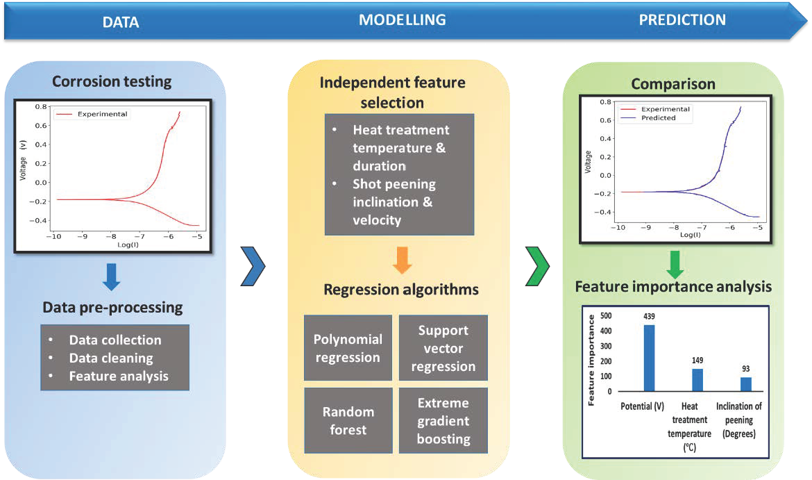
:This research work focuses on machine-learning-assisted prediction of the corrosion behavior of laser-powder-bed-fused (LPBF) and postprocessed Inconel 718. Corrosion testing data of these specimens were collected and fit into the following machine learning algorithms: polynomial regression, support vector regression, decision tree, and extreme gradient boosting. The model performance, after hyperparameter optimization, was evaluated using a set of established metrics: R2, mean absolute error, and root mean square error. Among the algorithms, the extreme gradient boosting algorithm performed best in predicting the corrosion behavior, closely followed by other algorithms. Feature importance analysis was executed in order to determine the postprocessing parameters that influenced the most the corrosion behavior in Inconel 718 manufactured by LPBF.

1. Summary
Inconel 718, a prominent member of the nickel-based superalloy family, is known for its strength, fatigue life, structural stability at elevated temperatures, and corrosion resistance [1,2,3,4,5]. Consequently, it is widely adopted in the aerospace and oil and gas industries [6,7,8,9,10]. This material meets the demands of the manufacturing industry by being amenable to casting, welding, and forming but continues to pose challenges during machining. As investigated by Amigo et al., In718 produces smoother finished parts when using oil-based emulsion rather than cryogenic cooling [11]. Apart from the traditional manufacturing methods, selective laser melting has become a popular additive manufacturing technology by which geometrically complex parts of this material are produced [12,13,14,15,16]. As a demonstration of this fact, replicative octahedral structures of different sizes have been manufactured using the LPBF technique by Ochoa et al. [17]. Further, this printed part has been tested for compressive loads using FEM simulation and validated using experimental testing for the purpose of aerospace light weighting. Laser powder bed fusion (LPBF) involves the layer-by-layer melting of metallic powder that consolidates to form the required solid present in the design [18,19,20,21]. After the printing process is completed, surface and heat treatments are carried out in order to smoothen the part and enhance microstructural homogeneity [22,23,24,25,26]. As this manufacturing technique allows better geometric freedom than the subtractive and mass-containing techniques, it is used for the fabrication of equipment used in oil and gas processing industries. A few examples are mud motor modules, subsurface valve components, and pump manifolds. Since the drilling and extraction environment contains high-pressure and high-temperature chlorides and contaminants, the material tends to disintegrate due to corrosion. Corrosion testing plays a vital role in the quality assessment of these parts [27,28,29]. A persistent challenge in this domain is to design corrosion testing techniques that produce accurate, industry-relevant results and thereby aid in lifetime extension. Electrochemical corrosion measurement is one of the established methods that performs testing under a simulated environment consisting of the tested material and the environment [30,31,32,33]. Potentiodynamic polarization (PD) measures the electrochemical activity in the cell, indicating the corrosion activity present in the material–environment combination [34,35,36]. The evolution of the corrosion potential is an important indicator in the understanding of long-term corrosion of the metallic alloy. Electrochemical impedance spectroscopy (EIS) analysis measures the stability of the passive layer formed when a material is exposed to an aggressive environment [37,38,39]. These two testing methods, put together, give us a picture of the rate at which the material is likely to corrode and the nature of the protective layer formed over the surface of materials upon reacting with the environment.
The data collected from the above experiments can be utilized to build machine learning (ML) models that predict the corrosion behavior of this material in the tested environment [40,41]. Machine learning algorithms are capable of performing multiple tasks, such as regression, classification, clustering, and dimensionality reduction, each finding its own application in the field of materials science [42,43,44,45]. Model development consists of three important steps: data preprocessing, algorithm adoption, and model testing and verification [46,47]. Data preprocessing refers to steps involving collection, cleaning, and organizing raw data. Algorithm adoption involves choosing the right type of algorithm based on the type of output required. Model testing and verification is the final step wherein the predictive capability of the model is tested and modified based on the errors arising. Many researchers are beginning to explore the adoption of ML models for accelerated material property prediction. Using the support vector regression algorithm (SVM) and back propagation neural network (BPNN), Wen et al. [48] predicted the rate of corrosion in steel alloy exposed to a seawater environment. Particle swarm optimization is used for parametric tuning in the SVM algorithm, and it has consistently outperformed the BPNN algorithm. LOOCV (leave-one-out cross validation) was adopted to validate the efficiency of the model. Kamrunnahar et al. [49] predicted the corrosion behavior of metallic glasses using polarization curves, carbon steel using weight loss data, and titanium alloy using crevice corrosion data, all collected from available literature. The BPNN network was able to capture the polarization behavior for a series of metallic glasses from the data of a single-member alloy. Compositional element details were used to model the corrosion rates in plain carbon steel and steel alloy. A good agreement was found between the experimental and estimated results. In another attempt to model the electrochemical behavior of an alloy system, Gong et al. [50] built machine learning models using several algorithms, such as k-nearest neighbor, decision tree, random forest, SVM, and gradient boosting decision tree algorithms. These models were then tested using corrosion data obtained for copper in a repository environment. The random forest algorithm produced the model closest to the experimental data. Feature importance analysis showed that sulfide concentration influenced the corrosion potential the most, and temperature influenced the impedance behavior the most. A more recent set of machine learning models for EIS analysis was built by Zhu et al. [51]. Literature data available for the electrical equivalent circuit (EEC) model for EIS analysis was adopted in the SVM algorithm. After the model “trained”, it was satisfactorily able to produce an EEC model upon providing the impedance data. This greatly reduces the human effort required in modelling the EEC. As the literature survey suggests, machine learning has the potential to grow into a beneficial tool that can expedite material behavior prediction. Most of these ML approaches are confined to cast or wrought material and have not been, to the authors’ knowledge, extended to selective-laser-melted material. Further, when compared with prior research, this study focuses on a unique form of corrosion data, the results of an electrochemical testing environment. The motivation for conducting this study is to develop a predictive model that can predict the corrosion behavior of an LPBF component and mathematically compute the contribution arising from each postprocessing treatment in the additive processing cycle. Currently, as LPBF is being optimized for wide-scale industrial adoption, understanding the role of postprocessing could facilitate the improvement of the product quality. Although this method of manufacturing has multiple advantages, it is, presently, expensive [52]. When machine learning is brought in to complete the prediction, the process becomes expedient, convenient, and cost-efficient.
In this work, machine learning algorithms were used to predict the electrochemical behavior of Inconel 718 produced via the additive route. For the purpose of model development, data were collected from one of our earlier experiments. Four machine learning models, decision tree (RF), extreme gradient boosting (XGB), support vector machine (SVM), and polynomial regression (PR) algorithms, were built using the collected data. The independent features considered were heat treatment temperature and duration, shot peening inclination and velocity, and individual input electrical parameter for each test. The performances of the ML models were evaluated, and the best-performing algorithm was employed to carry out feature importance analysis. Feature importance analysis performs the function of ranking the independent features for each of the electrochemical tests. This analysis is essential for determining the postprocessing parameters that largely influence the corrosion behavior of LPBF-processed Inconel 718.
2. Data Description
In order to collect data for building the machine learning model, corrosion experiments were conducted on selective-laser-melted and postprocessed Inconel 718 samples. These samples were divided into four categories: as built (AB), heat treated (HT), shot peened (SP), and heat treated with shot peening (HTSP). A detailed description of the experiment has been reported elsewhere [53]. A brief description of the printing process reported earlier in our work is provided below (https://0-www-mdpi-com.brum.beds.ac.uk/2075-4701/10/12/1562 (accessed on 5 May 2021).
The Inconel 718 specimens were printed vertically in small rectangular blocks with dimensions of 15 mm × 5 mm × 15 mm in an EOS M280 machine. The printer was equipped with a 200 W YB optical fiber laser with a beam diameter of 100 µm. Using a layer thickness of 20 µm and a scanning speed of 7 m/s, the blocks were printed with the 5 mm side as the base side. The printing chamber was enclosed in an argon atmosphere in order to prevent reactions between IN718 powder and the atmosphere. The powder supply to the printing region is enabled by the upward movement of the powder delivery system. When the requisite amount of powder is available, the recoater blade spreads the metallic powder on the build platform. In the equipment utilized for the current experiments, the recoater blade moved at a speed of 50 mm/s. The laser beam moved along the programmed path in order to melt the powder in the designed contour. After the current layer was completed, the next layer was spread again, and this procedure repeated until the object was printed completely. After the completion of the printing procedure, the build plate was removed, and the blocks were cut from the plate using a wire-cut electrodischarging machine.
A summary of the experimental conditions is presented in Table 1.
The postprocessing conditions are summarized in Table 2.
The specimens, thus printed, postprocessed, and categorized, were tested for general corrosion using an electrochemical method. The data from these tests represented the overall corroding tendency and passivation strength of the specimen. After running the tests four times to ensure reproducibility, data pertaining to PD and EIS analysis were collected in all four specimen conditions. Two of the electrochemical parameters that represented the corrosion activity in the PD test were Icorr and Epit. A lower Icorr represented lesser corrosion, and a higher Epit value represented improved passivating behavior. This trend was reflected by the HTSP specimen, with Icorr and Epit values of 0.04 µA/cm2 and 570 mV, respectively. The as-built specimen, offering the least corrosion resistance, possessed an Icorr value of 0.21 µA/cm2 and an Epit value of 220 mV. In the EIS testing, the passivation strength of the protective film was measured using the impedance of the film. It was found to be the least in the as-built specimen at 235 kΩ and the highest in the HTSP specimen at 682.2 kΩ. Heat treatment and shot peening, both forms of postprocessing, contributed to the enhancement of corrosion resistance of the selective-laser-melted Inconel 718. The laves phase distribution was reduced by the heat treatment process, thereby reducing the chromium depletion in the matrix. The high surface roughness of the samples, usually found in selective-laser-melted parts, was greatly reduced due to the shot peening process that consequently reduced the pitting tendency of the material.
2.1. Model Building
Database
The experimental electrochemical results thus obtained from the tests were categorized as Tafel plot, Bode plot, and Nyquist plot. The curves pertaining to these plots consisted of individual data points. For each individual input data point, a corresponding output data point was generated. In this manner, datasets formed for each sample condition was created. These datasets were utilized for model generation and corrosion behavior prediction.
2.2. Feature Selection
While building a predictive model, it is important to select the input features that contribute to the target variable the most [54,55,56]. All the present variables might not influence the outcome, and hence, the most causative parameters need to be carefully picked to improve the predictive capability of the model. In the current model, the postprocessing parameters and input parameters for each test were taken as independent variables. The target parameters also varied for each test, and these parameters are presented in Table 3, Table 4 and Table 5.
2.3. Model Development
A series of models were built for the four specimen conditions, namely, AB, HT, SP, and HTSP, for the three electrochemical plots in four different algorithms. The train, validation, and test data split adopted are as follows: train data set = 70% (to train the model behavior), validation data set = 15% (for hyperparameter tuning), test data set = 15% (for unbiased evaluation of the model performance). The number of data points used for model building was 29,100. Scikit-learn library was used for algorithm adoption, and the programming was carried out in Python language. A brief mathematical basis of each algorithm is provided in the following section.
2.3.1. Polynomial Regression
Polynomial regression (PR) [57,58] is a special case of linear regression where a polynomial equation is fitted on the data with a curvilinear relationship between the target variable and the independent variables. The features consist of all polynomial combinations of the features with a degree less than or equal to the specified degree.
where ε is the error. Similar to linear regression, the objective is to minimize the ordinary least squares sum.
Yi = θ0 + θ1xi + θ2xi2 + θ3xi3 + … + θnxin + ε
Minimizing the function:
{½*Σi(Y − Σjθjxij)2}
2.3.2. Support Vector Regression
Support vector regression (SVR) is a supervised regression algorithm with the advantage of controlling the deviation between the actual and predicted values to find an appropriate hyperplane to fit the data [59]. Unlike linear regression, SVR minimizes the squared sum of coefficients of the model.
Minimizing the function:
Constraining,
where ε is the maximum deviation or the margin length, |ζ| is the absolute deviation from the margin, and C is the regularization parameter. To capture the nonlinear relationship, the RBF kernel is employed. If the original feature space is represented by the vector, X = [x1,x2,x3,...,xn], then for any two datapoints A and B, the transformed feature space, ϕ(X), follows the condition,
where ||.||2 is the L2 norm and γ is the scaling parameter. The RBF kernel decreases with distance and ranges between zero (when ||A − B||2 tends towards infinity) and one (when A = B), which gives a ready interpretation as a similarity measure. Because of the nonlinearity introduced by the RBF kernel, the curve is linear in the ϕ(X) feature space.
|Y − Σθixi| < ε + |ζi|
ϕT(A)ϕ(B) = exp(−γ||A − B||22)
2.3.3. Decision Tree
Decision tree regression (DT) is a supervised regression algorithm that learns the set of decision rules for segmenting the features [60]. After segmenting the feature space, a constant piecewise approximation, such as the local average, is used for the prediction. The decision tree is built by recursive partitioning, with the root node (as the first parent) as the complete training dataset and the split data as the child nodes. These child nodes can be further split, considering them as new parent nodes. The node splitting is performed based on the mean squared error minimization. When a node S is split into A and B, the split value is determined as follows.
Minimizing the function:
where
The split value is obtained by minimizing the total mean squared loss of child nodes A and B, with the prediction in each of the child nodes as the sample mean of the respective node.
2.3.4. Extreme Gradient Boosting
Extreme gradient boosting (XGB) is a tree-based boosting ensemble method [61]. It is an evolved form of the boosting algorithm [62] formulated for enhanced predictive performance through optimization [63]. The objective function is given by the sum of loss function and regularization term as expressed using Equation (9).
where, l = loss function representing the difference between actual value (yi) and predicted (pi) value, and the regularization term Ω (fk) is given by
where T is the number of trees, w is the leaf weight, γ is the pruning index, and λ is the scaling factor of the weights.
Ω (fk) = γT + (0.5) ((λ) (w2))
If pi is the prediction at the t-th instance, we add an additional function ft (xi) in order to minimize the objective function. The objective function at the t-th iteration now becomes
The first and second orders derivative of the Taylor approximation function is used to solve Equation (6) and given as Equation (12).
Eliminating the constants, the equation now becomes
As can be seen from Equation (8), the objective function is dependent on the g and h values and hence becomes the optimization goal for the subsequent tree. In this manner, every loss function thus becomes optimized. The g and h values are calculated for each tree and placed in the corresponding leaf, and the values are added together by using the formula to identify a good tree.
2.4. Hyperparameter Optimization
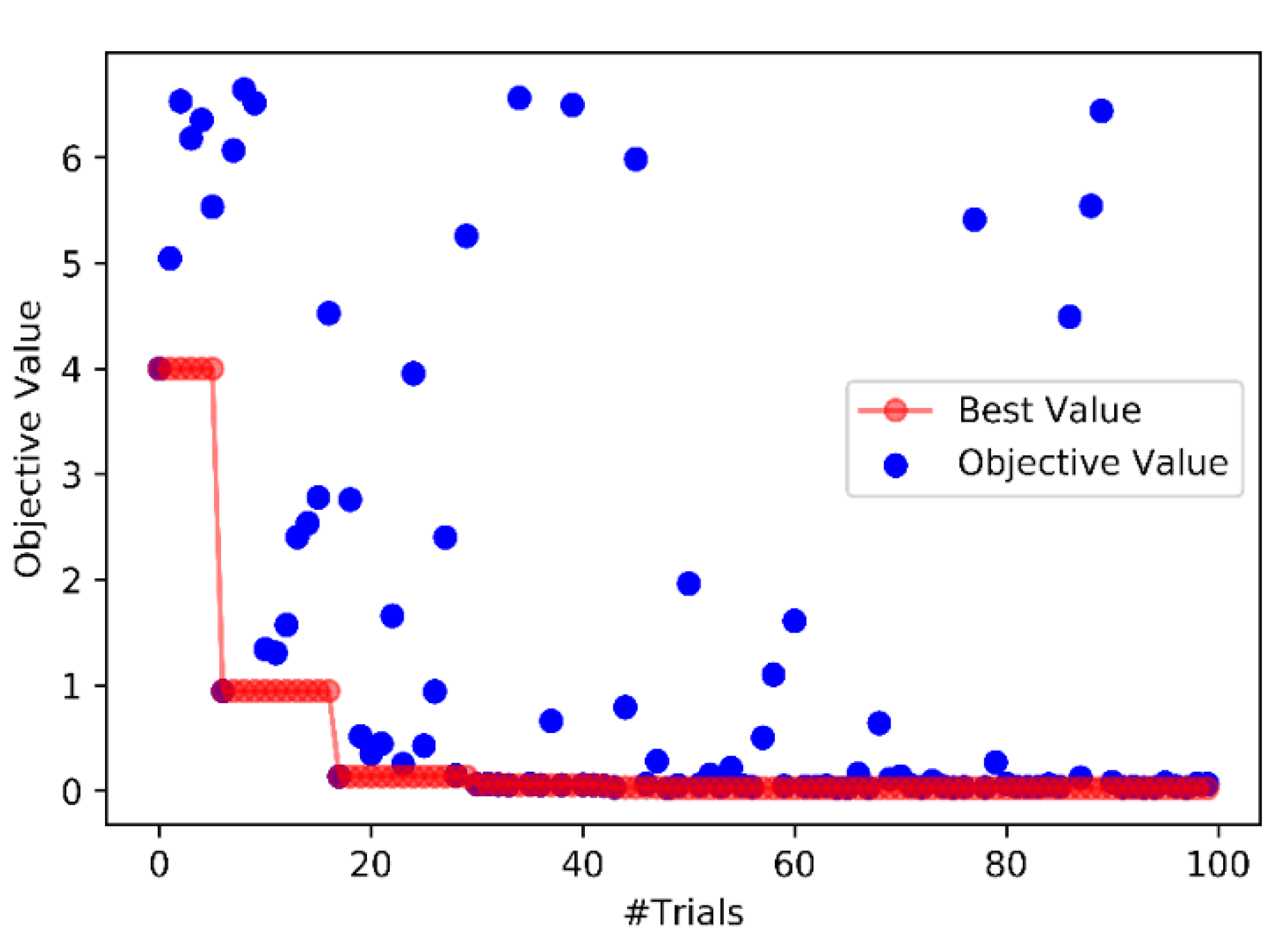
In order to obtain the best set of parameters that predicts the corrosion behavior closest to the experimental values, Bayesian optimization is performed over the hyperparameter space to minimize the root mean square error. Let H represent the overall hyperparameter space to be searched and h be a vector from the {H} space. Let O be the objective function to be minimized (i.e., root mean square error (RMSE)). In the Bayesian approach, P(O|h) is used for hyperparameter sampling and updated iteratively to get h* (best set of hyperparameters). In the probabilistic view, to calculate the improvement in performance between two consecutive iterations, the expected improvement metric (EI) is used:
where O* is the threshold value or the current best value of the objective function.
According to Bayes rule,
p(O|h) = p(h|O) ∗ (p(O)/p(h))
Here, p (h|O) is the probability of the hyperparameters given the score on the objective function, which is represented as follows:
p( h|O) = l(h) ifO < O*
On applying this expression, we can infer that EI is directly proportional to l(h)/g(h). Hence, to maximize EI, more samples need to be drawn from l(h) than g(h). As l(h) corresponds to O < O*, the objective function is bound to decrease. This algorithm is called the tree-structured Parzen estimator (TPE). To run this algorithm in a parallel manner, the asynchronous successive halving algorithm (ASHA) is used for pruning in every iteration. The least RMSE was obtained by the XGBoost algorithm for the PD, Nyquist, and Bode plots, and the hyperparameters were optimized using the Optuna package.
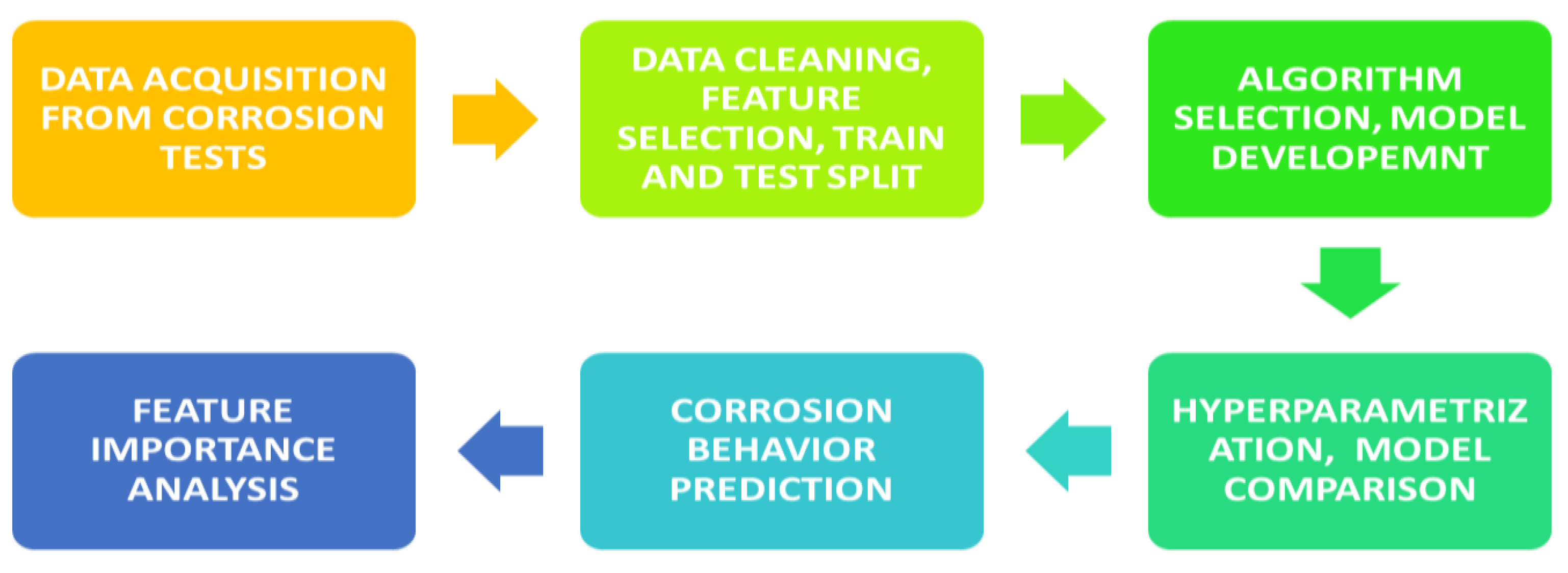
Figure 1 represents the optimization process graphically, adopted for the PD modelling. As can be seen, the objective value approaches the best value more closely as the number of trials keeps increasing. The individual parameters after the optimization are listed in Table 6. The model development process flow is presented in Figure 2.
3. Methods
3.1. Model Validation
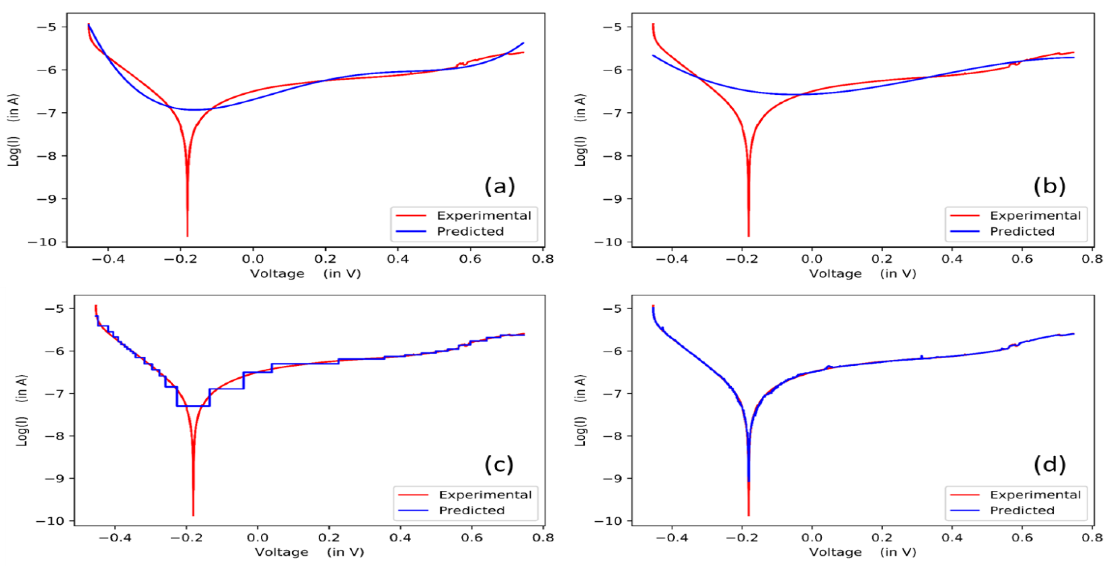
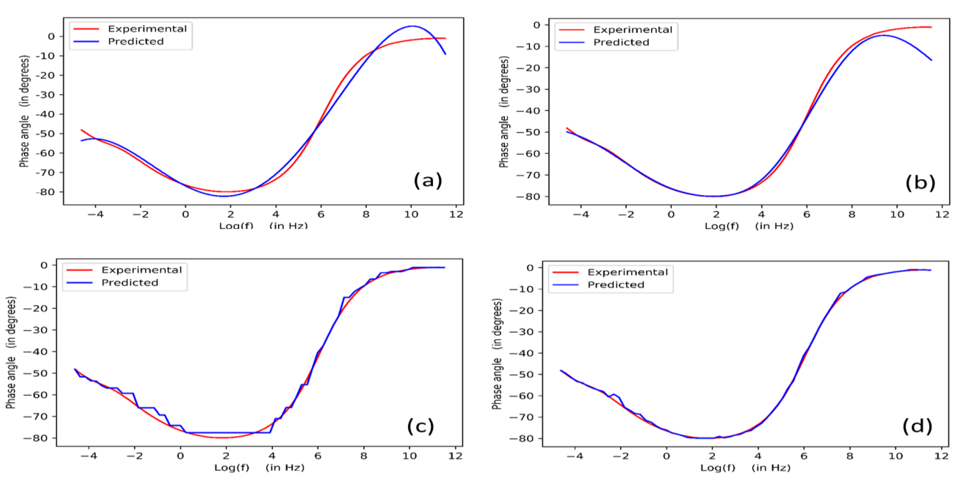
Once the models are developed using the different ML algorithms, the predicted results are compared with the experimental results. For this purpose, the experimental and predicted curves are drawn together to assess the deviation occurring in each model. The closer the curves are, the stronger is the predicting ability of the model. As discussing the results of each model in all the four experimental conditions is beyond the scope of this paper, the result of the HTSP condition, the specimen condition that contained the highest corrosion resistance, is being presented. Models of the other experimental conditions, namely, AB, HT, and SP, may be found at the following URL: https://github.com/rohithsrinivaas/Corrosion_Informatics (accessed on 21 May 2021) The experimental and predicted results of the PD and EIS plots are shown in Figure 3, Figure 4 and Figure 5. In Figure 2, all the models are able to perform prediction fairly closely in both the cathodic and anodic regions. The deviations are more apparent in the region where it dips towards the Ecorr value. As can be seen in Figure 3d, the XGB model curve remains closest to the experimental data. The curve fitting of the other models, PR, SVM, and DT, are unable to capture the polarization behavior accurately. This is because these algorithms are unable to predict the data region where the shift towards the Ecorr value occurs. In the PR model, as shown in Figure 3a, as the data are modelled as a smooth polynomial function, the trend change in the Tafel curve becomes difficult to predict. Similarly in the SVM model shown in Figure 3d, the kernel used is a continuous and smooth transformation of the input feature space, and the prediction curve is more of a gradual dip as against the pointed dip in experimental data. The DT model has slightly better accuracy in capturing the data trend in regions surrounding the Ecorr value, as depicted in Figure 3c. Though the accuracy is higher, the predicted curve is a stepwise combination of straight line segments rather than a smooth curve. This is because the DT algorithm is driven by piecewise constant approximation. The XGB model is able to predict the data shift region accurately, with a prediction curve almost the same as the experimental curve. The effect of this can be observed in the prediction of the Bode and Nyquist plots, as shown in Figure 4c and Figure 5c. The experimental curves are approximated more as flat lines in this model. In the EIS analysis as well, in both the Bode and Nyquist plots, the XGB model is able to predict the data more accurately when compared with the other algorithms. This is due to error minimization that occurs in every step of model building, otherwise known as the regularization term. This algorithm “learns” the error or deviation of the previous right and corrects it in the subsequent step. It also has the additional advantages of parallel tree building and parametric tuning that optimizes the tree depth and nodes.
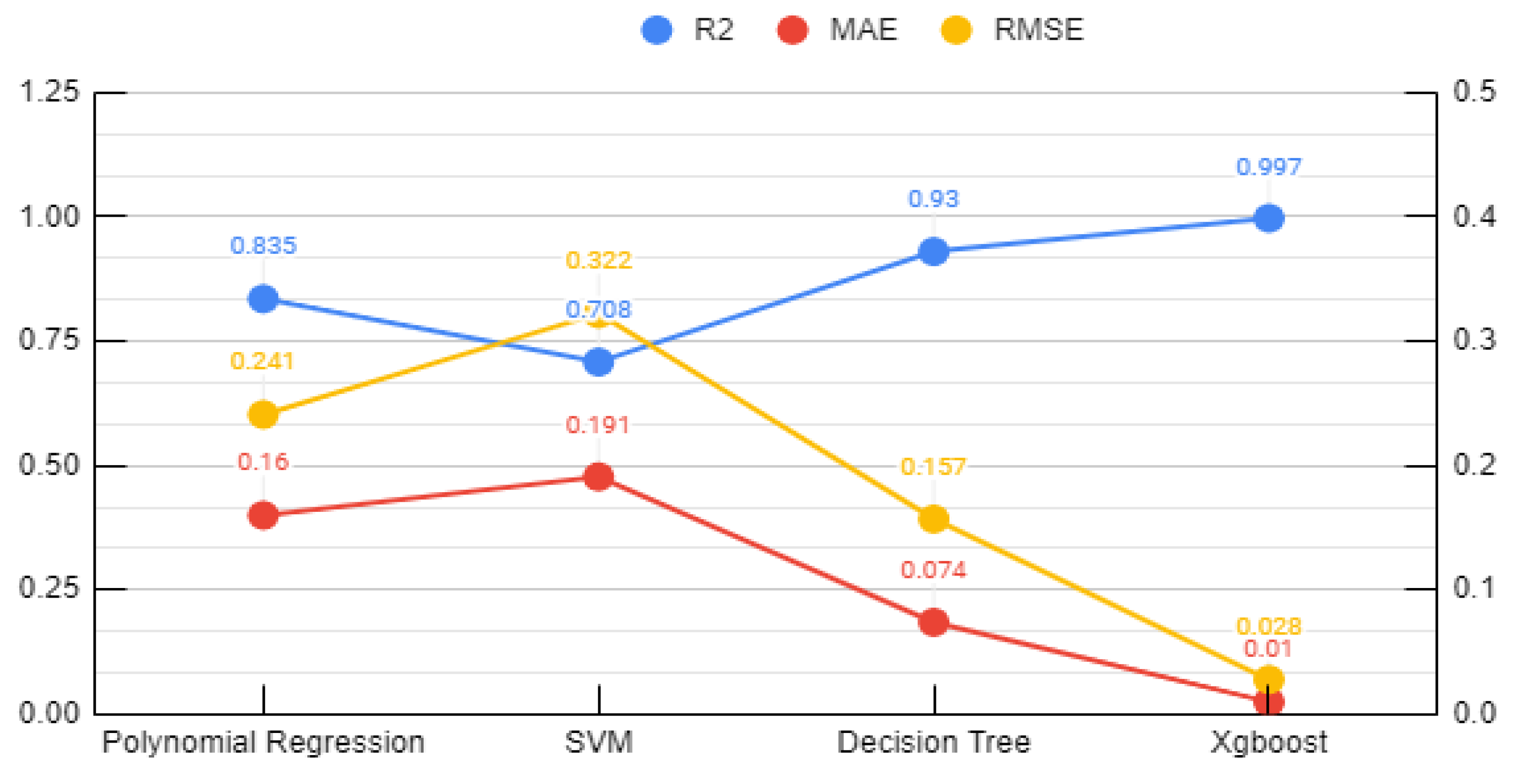
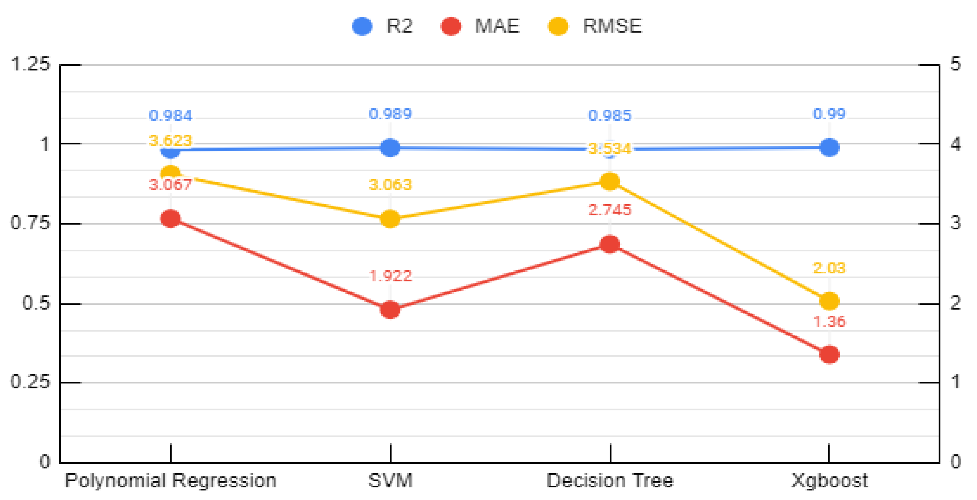
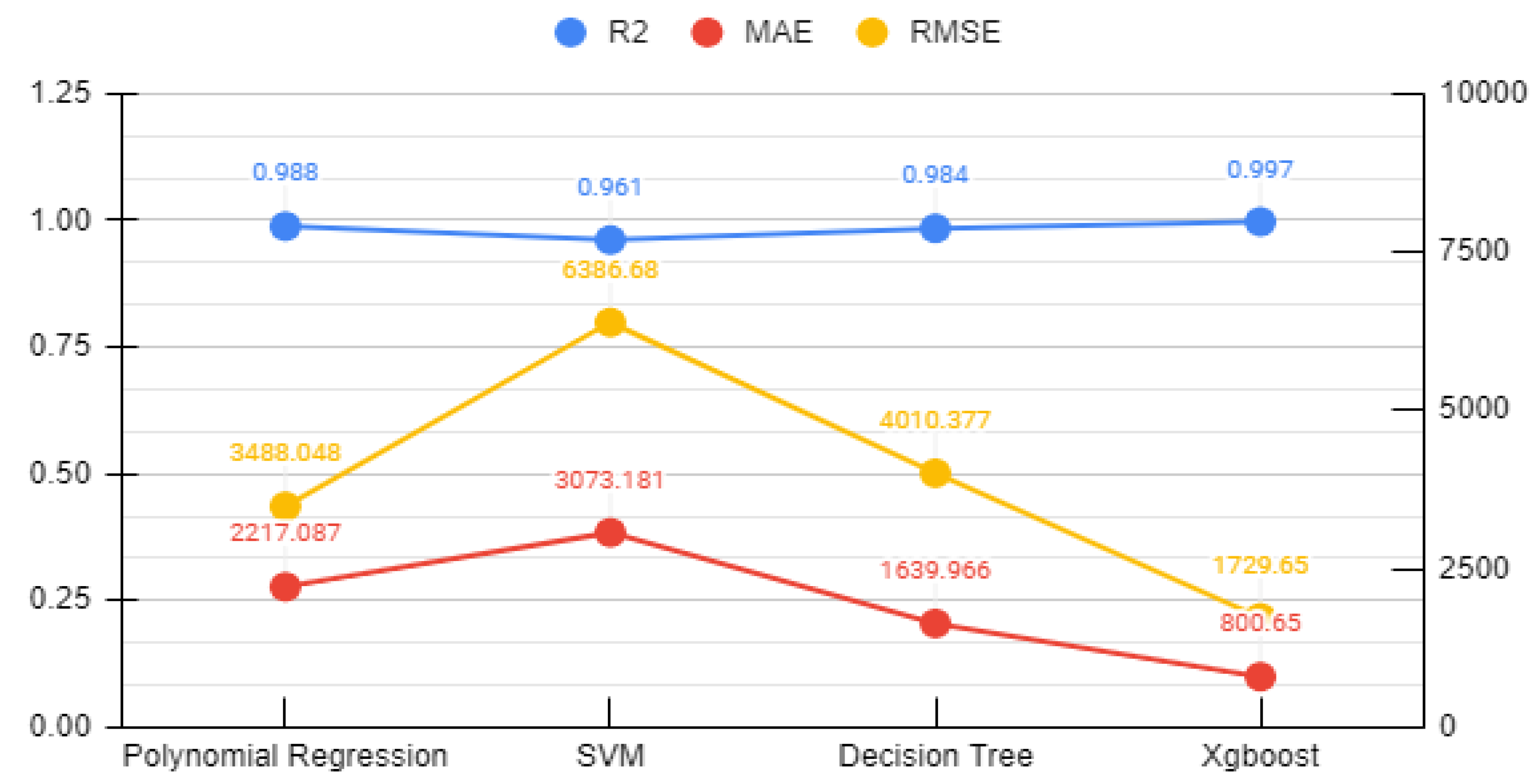
The model accuracy is determined by certain established metrics, such as R2, MAE (mean absolute error), and RMSE (root mean square error). In the potentiodynamic polarization testing, it can be seen that R2 is the highest for the XGB model at 0.954. It is distinctively higher than the other algorithms. The DT algorithm performs the second best at 0.93. The SVM model has the lowest value at 0.708, representing a poor prediction capability. This shows that this model cannot satisfactorily calculate the variations occurring during the electrochemical reaction of corrosion. This is in line with the results of the experimental versus predicted graph depicted for SVM. In the EIS analysis, the Bode plot prediction has all the algorithms performing almost at the same level, with PR at 0.984, SVM at 0.989, DT at 0.0.985, and XGB at 0.99. Though the differences are minor, it can be seen that XGB outperformed the other models. In the prediction for the Nyquist plot too, it is observed that XGB has the highest R2 score of 0.997 and SVM performs the poorest at 0.961.
The metrics MAE and RMSE are considered to be better when they are lower. When comparing these metrics for the PD plot, as shown in Figure 6, SVM has the highest MAE value of 0.191 and RMSE value of 0.322. Other algorithms performed better with PR at a MAE value of 0.16 and RMSE value of 0.241. Decision tree has a slightly better score of 0.074 than XGB at 0.077. This is the only metric in which DT outclassed the XGB algorithm. In the Bode plot prediction, the lowest MAE (1.98) belongs to SVM, closely followed by XGB at 2.16, as can be seen in Figure 7. The least RMSE score of 2.9 is given by XGB. In the Nyquist plot prediction as well, the errors of least value was given out by XGB, as presented in Figure 8. Overall, it is clear that the experimental plots were best matched by the XGB algorithm, its prediction efficiency reflected in both the comparisons and error analysis.
3.2. Feature Importance Analysis
Feature importance analysis is carried out to determine the independent features that influence the outcome the most. As the XGB model performed best in prediction, this model is used for feature importance analysis in the PD and EIS experiments. This result is presented in Figure 9. The potentiodynamic polarization testing relates the material’s sensitivity to the corrosion process. The results, as can be seen in Figure 9a, show that the input potential value is the most significant parameter that influences the outcome. As the polarization current is primarily controlled by the input potential, the corrosion activity is also dependent on it. The second most influential parameter is the heat treatment temperature. The temperature of heat treatment plays a dominant role in deciding the microstructure, which in turn influences the corrosion behavior of the material. As Inconel 718 is a precipitation-strengthened alloy, the distribution and formation of the phases, such as γ’, γ”, and δ, determine how strong it can remain in an aggressive environment. The precipitation of laves phase occurring during the melting process tends to deplete the γ matrix of the chromium content. As discussed in our previous work, the network of laves phase is reduced due to the heat treatment, and this helps in increasing the chromium content in the main matrix. This is one of the main reasons heat-treated samples show an improved corrosion resistance when compared with the as-built sample. A similar improvement was reported by Luo et al. [64]. Additively manufactured Inconel 718 samples were subjected to different heat treatments, from 940 to 1020 ℃, with double ageing. It was found that an increase in the heat-treating temperature led to a decreased tendency of the laves phase to micro-segregate, and this resulted in a noticeable improvement in the passive layer formation. The passive layer that formed in the as-built specimen quickly disintegrated, while the heat-treated specimens formed a more strongly adherent layer, exhibited by the higher Epit values. Li et al. [65] additionally inferred that the fine δ phase pinning effect on the grain boundary is caused by heat-treating selective-laser-melted Inconel 718. This effect leads to more electrochemical homogeneity, thereby bringing down the Icorr value when these samples were tested in a NaCl environment. In other metal additive manufacturing techniques too, analogous results were found. When heat-treating electron-beam-smelted samples of Inconel 718, You et al. [14] found that a temperature of 1150 °C increased the pitting resistance due to the higher precipitation of γ’ and γ”. An increase in the solution-treating temperature also led to a more uniform distribution of γ’ particles. A judicious conclusion can hence be arrived that heat treatment helps in establishing a higher corrosion resistance in SLMed material of this alloy.
When analyzing the feature importance plot for the EIS experiments, it is seen that, here also, the input electrical parameter influences the outcome the maximum, as can be seen in Figure 9b,c. Apart from that, it can be seen that the inclination of shot peening is the second dominant factor. Shot peening is a commonly adopted procedure to introduce beneficial compressive stresses and reduce the surface irregularities and consequently crack initiation [66]. The favorable topographical changes introduced in the surface is also an added advantage of this technique. As EIS testing relates to the strength of the passive layer, it is highly possible to suggest that a smoother surface, with reduced irregularities, remains stronger. One shot peening parameter that is directly connected to the resulting surface level changes is the inclination at which the spherical balls hit the material. It determines the angle of contact between the peening and work material, area of contact, and friction levels. If the contact angle is too acute, too much material could be removed, resulting in dimensional alterations. If the contact angle is too obtuse, it might not be very effective in smoothening the target material. Hence, an optimum angle of 45° is chosen for the shot peening process. The importance of the angle of inclination in the strength of the passive layer was correctly identified by the built model in the EIS plots. Hence, it can be said that the machine learning model not only is capable of predicting the experimental results accurately but also identified the influential independent parameters appropriately.
4. Conclusions
The present work adopted machine learning to predict the corrosion behavior of Inconel 718 manufactured by LPBF in both as-built and postprocessed conditions. Data were collected from the PD and EIS tests for all the experimental conditions and implemented in different ML algorithms. The following are the key conclusions of this work:
- Based on experimental data, the relationship between postprocessing techniques and corrosion resistance was explored using a machine learning approach. The feasibility of such an approach was demonstrated using four different ML algorithm namely, Polynomial regression, Support vector regression, Random forest and Extreme gradient boosting.
- In the development of ML-based models, the XGB algorithm led to the corrosion rate prediction of the alloy with the highest accuracy at an R2 value of 0.954 in PD testing and 0.997 in EIS testing.
- In the feature importance analysis, apart from the electrical parameters, heat treatment temperature and shot peening inclination were found to be the most influential parameters in determining the corrosion resistance of Inconel 718.
Since the optimization of processing and postprocessing parameters is still in the nascent stage in metal additive manufacturing, data-driven models can help in establishing the appropriate set of input variables. An effective property predictive model can improve the understanding of the complex dynamics of electrochemical mechanisms fordeveloping corrosion-resistant materials in various structural applications.
Author Contributions
Conceptualization—M.O.V.; methodology—M.O.V. and R.S.M.; software—R.S.M.; validation—R.S.M.; formal analysis—M.O.V. and R.S.M.; investigation—M.O.V.; resources—A.K.T.; data curation—M.O.V. and A.K.T.; writing—original draft preparation—M.O.V. and R.S.M.; writing—review and editing—J.R.; visualization—M.O.V. and J.R.; supervision—J.R.; project administration—J.R.; All authors have read and agreed to the published version of the manuscript.
Funding
Not supported by any funding agency.
Institutional Review Board Statement
Is not applicable for this study as it did not involve any human or animal subject.
Data Availability Statement
Conflicts of Interest
The authors declare no conflict of interest.
References
- Davis, J.R. ASM specialty handbook: Nickel, cobalt, and their alloys. Choice Rev. Online 2001, 38, 38–6206. [Google Scholar] [CrossRef]
- Pint, B.; Unocic, K.; Dryepondt, S. Oxidation of Superalloys in Extreme Environments. In Proceedings of the 7th International Symposium on Superalloy 718 and Derivatives (2010), Pittsburgh, PA, USA, 10–12 October 2010; pp. 861–875. [Google Scholar]
- Park, M. ASM Handbook Corrosion: Materials; American society of materials: Almere, The Netherlands, 2005. [Google Scholar]
- Akca, E.; Gürsel, A. A Review on Superalloys and IN718 Nickel-Based INCONEL Superalloy. Period. Eng. Nat. Sci. (PEN) 2017, 3. [Google Scholar] [CrossRef]
- Thomas, A.; El-Wahabi, M.; Cabrera, J.M.; Prado, J. High temperature deformation of Inconel 718. J. Mater. Process. Technol. 2006, 177, 469–472. [Google Scholar] [CrossRef]
- Mishra, A. Performance of Corrosion-Resistant Alloys in Concentrated Acids. Acta Met. Sin. Engl. Lett. 2017, 30, 306–318. [Google Scholar] [CrossRef] [Green Version]
- Soc, S.G.J.E. Corrosion of Steels and Nickel Alloys in Superheated Steam Corrosion of Steels and Nickel Alloys in Superheated Steam. J. Electrochem. Soc. 1964, 111, 1116. [Google Scholar]
- Delabrouille, F.; Legras, L.; Vaillant, F.; Scott, P.; Viguier, B.; Andrieu, E. Effect of the Chromium Content and Strain on the Corrosion of Nickel Based Alloys in Primary Water of Pressurized Water. In Proceedings of the 12th International Conference on Environmental Degradation of Materials in Nuclear Power System–Water Reactors, Salt Lake City, UT, USA, 14–18 August 2005. [Google Scholar]
- Mishra, A.K.; Shoesmith, D.W. Effect of Alloying Elements on Crevice Corrosion Inhibition of Nickel-Chromium-Molybdenum-Tungsten Alloys Under Aggressive Conditions: An Electrochemical Study. Corrosion 2014, 70, 721–730. [Google Scholar] [CrossRef]
- Cwalina, K.L.; Demarest, C.; Gerard, A.; Scully, J. Revisiting the effects of molybdenum and tungsten alloying on corrosion behavior of nickel-chromium alloys in aqueous corrosion. Curr. Opin. Solid State Mater. Sci. 2019, 23, 129–141. [Google Scholar] [CrossRef]
- Amigo, F.J.; Urbikain, G.; Pereira, O.; Fernández-Lucio, P.; Fernández-Valdivielso, A.; de Lacalle, L.L. Combination of high feed turning with cryogenic cooling on Haynes 263 and Inconel 718 superalloys. J. Manuf. Process. 2020, 58, 208–222. [Google Scholar] [CrossRef]
- Choi, J.-P.; Shin, G.-H.; Yang, S.; Yang, D.-Y.; Lee, J.-S.; Brochu, M.; Yu, J.-H. Densification and microstructural investigation of Inconel 718 parts fabricated by selective laser melting. Powder Technol. 2017, 310, 60–66. [Google Scholar] [CrossRef]
- Du, D.; Dong, A.; Shu, D.; Zhu, G.; Sun, B.; Li, X.; Lavernia, E. Influence of build orientation on microstructure, mechanical and corrosion behavior of Inconel 718 processed by selective laser melting. Mater. Sci. Eng. A 2019, 760, 469–480. [Google Scholar] [CrossRef]
- Baicheng, Z.; Xiaohua, L.; Jiaming, B.; Junfeng, G.; Pan, W.; Chen-Nan, S.; Muiling, N.; Guojun, Q.; Jun, W. Study of selective laser melting (SLM) Inconel 718 part surface improvement by electrochemical polishing. Mater. Des. 2017, 116, 531–537. [Google Scholar] [CrossRef]
- Li, H.; Feng, S.; Li, J.; Gong, J. Effect of heat treatment on the δ phase distribution and corrosion resistance of selective laser melting manufactured Inconel 718 superalloy. Mater. Corros. 2018, 69, 1350–1354. [Google Scholar] [CrossRef]
- Luo, S.; Huang, W.; Yang, H.; Yang, J.; Wang, Z.; Zeng, X. Microstructural evolution and corrosion behaviors of Inconel 718 alloy produced by selective laser melting following different heat treatments. Addit. Manuf. 2019, 30, 100875. [Google Scholar] [CrossRef]
- Calleja-Ochoa, A.; Gonzalez-Barrio, H.; de Lacalle, N.L.; Martínez, S.; Albizuri, J.; Lamikiz, A. A New Approach in the Design of Microstructured Ultralight Components to Achieve Maximum Functional Performance. Materials 2021, 14, 1588. [Google Scholar] [CrossRef]
- Almangour, B. Additive manufacturing of emerging materials. Addit. Manuf. Emerg. Mater. 2018, 1–355. [Google Scholar] [CrossRef]
- Debroy, T.; Wei, H.L.; Zuback, J.S.; Mukherjee, T.; Elmer, J.W.; Milewski, J.O.; Beese, A.M.; Wilson-Heid, A.D.; De, A.; Zhang, W. Additive manufacturing of metallic components–Process, structure and properties. Prog. Mater. Sci. 2018, 92, 112–224. [Google Scholar] [CrossRef]
- Kumar, S.; Pityana, S. Laser-Based Additive Manufacturing of Metals. Adv. Mater. Res. 2011, 227, 92–95. [Google Scholar] [CrossRef]
- Yap, C.Y.; Chua, C.K.; Dong, Z.; Liu, Z.H.; Zhang, D.Q.; Loh, L.E.; Sing, S.L. Review of selective laser melting: Materials and applications. Appl. Phys. Rev. 2015, 2, 041101. [Google Scholar] [CrossRef]
- Kaynak, Y.; Tascioglu, E. Post-processing effects on the surface characteristics of Inconel 718 alloy fabricated by selective laser melting additive manufacturing. Prog. Addit. Manuf. 2020, 5, 221–234. [Google Scholar] [CrossRef]
- Raghavan, S.; Zhang, B.; Wang, P.; Sun, C.-N.; Nai, M.L.S.; Li, T.; Wei, J. Effect of different heat treatments on the microstructure and mechanical properties in selective laser melted INCONEL 718 alloy. Mater. Manuf. Process. 2017, 32, 1588–1595. [Google Scholar] [CrossRef]
- Chen, L.; Sun, Y.; Li, L.; Ren, X. Microstructural evolution and mechanical properties of selective laser melted a nickel-based superalloy after post treatment. Mater. Sci. Eng. A 2020, 792, 139649. [Google Scholar] [CrossRef]
- Zhao, Y.; Guo, Q.; Ma, Z.; Yu, L. Comparative study on the microstructure evolution of selective laser melted and wrought IN718 superalloy during subsequent heat treatment process and its effect on mechanical properties. Mater. Sci. Eng. A 2020, 791, 139735. [Google Scholar] [CrossRef]
- Kermani, M.; Harrop, D. The Impact of Corrosion on Oil and Gas Industry. SPE Prod. Facil. 1996, 11, 186–190. [Google Scholar] [CrossRef] [Green Version]
- Finšgar, M.; Jackson, J. Application of corrosion inhibitors for steels in acidic media for the oil and gas industry: A review. Corros. Sci. 2014, 86, 17–41. [Google Scholar] [CrossRef] [Green Version]
- Tiu, B.D.; Advincula, R.C. Polymeric corrosion inhibitors for the oil and gas industry: Design principles and mechanism. React. Funct. Polym. 2015, 95, 25–45. [Google Scholar] [CrossRef]
- Groysman, A. Corrosion for Everybody; Springer: Berlin/Heidelberg, Germany, 2010; pp. 189–190. [Google Scholar] [CrossRef]
- Meade, C.L. Accelerated corrosion testing. Metal Finish. 2000, 98, 540–545. [Google Scholar] [CrossRef]
- Lorenz, W.J. Determination of corrosion rates by electrochemical DC and AC methods. Corros. Sci. 1981, 21, 647–672. [Google Scholar] [CrossRef]
- Mansfeld, S.F.; Tsai, I. Weight Studies of Atmospheric Corrosion—Loss and Electrochemical Measurements. Corros. Sci. 1980, 20, 1–3. [Google Scholar] [CrossRef]
- Sjding, A.B.J. Corrosion testing by potentiodynamic polarization in various electrolytes. Corros. Sci. 1992, 241–245. [Google Scholar]
- Mansfeld, F. Tafel slopes and corrosion rates obtained in the pre-Tafel region of polarization curves. Corros. Sci. 2005, 47, 3178–3186. [Google Scholar] [CrossRef]
- McCafferty, E. Validation of corrosion rates measured by the Tafel extrapolation method. Corros. Sci. 2005, 47, 3202–3215. [Google Scholar] [CrossRef]
- Chang, B.-Y.; Park, S.-M. Electrochemical Impedance Spectroscopy. Annu. Rev. Anal. Chem. 2006, 3, 207–229. [Google Scholar] [CrossRef]
- Agarwal, P.; Orazem, M.E.; Garcia-Rubio, L.H. Measurement models for electrochemical impedance spectroscopy: I. Demonstration of applicability. J. Electrochem. Soc. 1992, 139, 1917. [Google Scholar] [CrossRef]
- Park, S. With impedance data, a complete description of an electrochemical system is possible. Anal. Chem. 2003, 75, 455–461. [Google Scholar]
- Yu, X. Machine learning application in the life time of materials. arXiv 2017, arXiv:1707.04826. [Google Scholar]
- Irani, M.; Chalaturnyk, R.; Hajiloo, M. Application of data mining techniques in building predictive models for oil and gas problems: A case study on casing corrosion prediction. Int. J. Oil Gas Coal Technol. 2014, 8, 369–398. [Google Scholar] [CrossRef]
- Liu, Y.; Zhao, T.; Ju, W.; Shi, S. Materials discovery and design using machine learning. J. Mater. 2017, 3, 159–177. [Google Scholar] [CrossRef]
- Butler, K.T.; Davies, D.W.; Cartwright, H.; Isayev, O.; Walsh, A. Machine learning for molecular and materials science. Nat. Cell Biol. 2018, 559, 547–555. [Google Scholar] [CrossRef]
- Roh, Y.; Heo, G.; Whang, S.E. A Survey on Data Collection for Machine Learning. IEEE Trans. Knowl. Data Eng. 2019, 4347, 1–20. [Google Scholar] [CrossRef] [Green Version]
- Schmidt, J.; Marques, M.R.G.; Botti, S.; Marques, M.A.L. Recent advances and applications of machine learning in solid-state materials science. NPJ Comput. Mater. 2019, 5. [Google Scholar] [CrossRef]
- Yang, Q.; Liu, Y.; Chen, T.; Tong, Y. Federated Machine Learning: Concept and Applications. ACM Trans. Intell. Syst. Technol. 2019, 10, 1–19. [Google Scholar] [CrossRef]
- Sutton, C.; Boley, M.; Ghiringhelli, L.M.; Rupp, M.; Vreeken, J.; Scheffler, M. Identifying domains of applicability of machine learning models for materials science. Nat. Commun. 2020, 11, 1–9. [Google Scholar] [CrossRef] [PubMed]
- Kailkhura, B.; Gallagher, B.; Kim, S.; Hiszpanski, A.; Han, T.Y.-J. Reliable and explainable machine-learning methods for accelerated material discovery. NPJ Comput. Mater. 2019, 5, 1–9. [Google Scholar] [CrossRef]
- Wen, Y.; Cai, C.; Liu, X.; Pei, J.; Zhu, X.; Xiao, T. Corrosion rate prediction of 3C steel under different seawater environment by using support vector regression. Corros. Sci. 2009, 51, 349–355. [Google Scholar] [CrossRef]
- Kamrunnahar, M.; Urquidi-Macdonald, M. Prediction of corrosion behavior using neural network as a data mining tool. Corros. Sci. 2010, 52, 669–677. [Google Scholar] [CrossRef]
- Gong, X.; Dong, C.; Xu, J.; Wang, L.; Li, X. Machine learning assistance for electrochemical curve simulation of corrosion and its application. Mater. Corros. 2019, 71, 474–484. [Google Scholar] [CrossRef]
- Zhu, S.; Sun, X.; Gao, X.; Wang, J.; Zhao, N.; Sha, J. Equivalent circuit model recognition of electrochemical impedance spectroscopy via machine learning. J. Electroanal. Chem. 2019, 855, 113627. [Google Scholar] [CrossRef] [Green Version]
- Watson, J.; Taminger, K. A decision-support model for selecting additive manufacturing versus subtractive manufacturing based on energy consumption. J. Clean. Prod. 2018, 176, 1316–1322. [Google Scholar] [CrossRef]
- Mythreyi, O.V.; Raja, A.; Nagesha, B.K.; Jayaganthan, R. Corrosion Study of Selective Laser Melted IN718 Alloy upon Post Heat Treatment and Shot Peening. Metals 2020, 10, 1562. [Google Scholar] [CrossRef]
- Cai, J.; Luo, J.; Wang, S.; Yang, S. Feature selection in machine learning: A new perspective. Neurocomputing 2018, 300, 70–79. [Google Scholar] [CrossRef]
- Vafaie, H.; De Jong, K. Genetic Algorithms as a Tool for Feature Selection in Machine Learning. In Proceedings of the IEEE International Conference on Tools with Artificial Intelligence, Arlington, VA, USA, 10–11 November 1992. [Google Scholar]
- Ostertagová, E. Modelling using Polynomial Regression. Procedia Eng. 2012, 48, 500–506. [Google Scholar] [CrossRef] [Green Version]
- Smola, A.J.; Schölkopf, B. A tutorial on support vector regression. Stat. Comput. 2004, 14, 199–222. [Google Scholar] [CrossRef] [Green Version]
- Czajkowski, M.; Kretowski, M. The role of decision tree representation in regression problems—An evolutionary perspective. Appl. Soft Comput. 2016, 48, 458–475. [Google Scholar] [CrossRef]
- Guttenberg, N. Learning to generate classifiers. arXiv 2018, arXiv:1803.11373. [Google Scholar]
- Zemel, R.S. A Gradient-Based Boosting Algorithm for Regression Problems. In Proceedings of the 13th International Conference on Neural Information Processing Systems, Hong Kong, China, 3–6 October 2006. [Google Scholar]
- Chen, T. XGBoost: A Scalable Tree Boosting System. In Proceedings of the 22nd Acm Sigkdd International Conference on Knowledge Discovery and Data Mining, San Francisco, CA, USA, 13–17 August 2016. [Google Scholar]
- You, X.; Tan, Y.; Zhao, L.; You, Q.; Wang, Y.; Ye, F.; Li, J. Effect of solution heat treatment on microstructure and electrochemical behavior of electron beam smelted Inconel 718 superalloy. J. Alloys Compd. 2018, 741, 792–803. [Google Scholar] [CrossRef]
- Mylonas, G.; Labeas, G. Numerical modelling of shot peening process and corresponding products: Residual stress, surface roughness and cold work prediction. Surf. Coat. Technol. 2011, 205, 4480–4494. [Google Scholar] [CrossRef]
- Bagherifard, S.; Ghelichi, R.; Guagliano, M. Numerical and experimental analysis of surface roughness generated by shot peening. Appl. Surf. Sci. 2012, 258, 6831–6840. [Google Scholar] [CrossRef]
- Walter, R.; Kannan, M.B. Influence of surface roughness on the corrosion behaviour of magnesium alloy. Mater. Des. 2011, 32, 2350–2354. [Google Scholar] [CrossRef]
- Kovacı, H.; Bozkurt, Y.; Yetim, A.; Aslan, M.; Çelik, A. The effect of surface plastic deformation produced by shot peening on corrosion behavior of a low-alloy steel. Surf. Coat. Technol. 2019, 360, 78–86. [Google Scholar] [CrossRef]
Figure 1.
Optimization history plot.

Figure 2.
Model development process flowchart.

Figure 3.
Comparison of PD results of models built in (a) PR, (b) SVM, (c) DT, and (d) XGB.

Figure 4.
Comparison of Bode results of models built in (a) PR, (b) SVM, (c) DT, and (d) XGB.

Figure 5.
Comparison of Nyquist results of models built in (a) PR, (b) SVM, (c) DT, and (d) XGB.

Figure 6.
Comparison of results among the algorithms in the PD plot.

Figure 7.
Comparison of results among the algorithms in the Bode plot.

Figure 8.
Comparison of results among the algorithms in the Nyquist plot.

Figure 9.
Feature importance ranking for the (a) PD plot, (b) Bode plot, (c) Nyquist plot.


Table 1.
Experimental conditions.
| Specimen Conditions | AB, HT, SP, HTSP |
|---|---|
| Corrosion testing methods used | Potentiodynamic polarization, electrochemical impedance spectroscopy |
| Postprocessing used | Heat treatment, shot peening |
| Testing environment | 3.5 wt% NaCl environment |
| Mode of corrosion tested | Aqueous, general corrosion |
| Data source | Gamry 600+, electrochemical workstation software |
| Corrosion plots used | PD, Bode, Nyquist |
Table 2.
Postprocessing conditions.
| Parameter | Value |
|---|---|
| Heat treatment temperature | 980 °C |
| Heat treatment duration | 15 min |
| Shot peening inclination | 45° |
| Shot peening velocity | 70 m/s |
Table 3.
Independent features for the PD plot.
| Independent Parameters for the Tafel Plot | |||||
|---|---|---|---|---|---|
| Sample Condition | Heat Treatment Temperature (°C) | Heat Treatment Duration (Min) | Shot Peening Velocity (m/s) | Shot Peening Inclination (Degrees) | Voltage (Volts) |
| AB | 0 | 0 | 0 | 0 | −4.77 × 10⁻¹ |
| HT | 980 | 15 | 0 | 0 | −4.74 × 10⁻¹ |
| SP | 0 | 0 | 70 | 45 | −4.27 × 10⁻¹ |
| HTSP | 980 | 15 | 70 | 45 | −4.71 × 10⁻¹ |
Dependent parameter—current (amps).
Table 4.
Independent features for the Bode plot.
| Independent Parameters for the Bode Plot | |||||
|---|---|---|---|---|---|
| Sample Condition | Heat Treatment Temperature (°C) | Heat Treatment Duration (min) | Shot Peening Velocity (m/s) | Shot Peening Inclination (Degrees) | Frequency (Hz) |
| AB | 0 | 0 | 0 | 0 | 79,450 |
| HT | 980 | 15 | 0 | 0 | 63,140 |
| SP | 0 | 0 | 70 | 45 | 50,200 |
| HTSP | 980 | 15 | 70 | 45 | 39,890 |
Dependent parameter—phase angle (degrees).
Table 5.
Independent features for the Nyquist plot.
| Independent Parameters for the Nyquist Plot | |||||
|---|---|---|---|---|---|
| Sample Condition | Heat Treatment Temperature (°C) | Heat Treatment Duration (min) | Shot Peening Velocity (m/s) | Shot Peening Inclination (Degrees) | Impedance {Real} (Ohm) |
| AB | 0 | 0 | 0 | 0 | 27.59 |
| HT | 980 | 15 | 0 | 0 | 31.05 |
| SP | 0 | 0 | 70 | 45 | 26.97 |
| HTSP | 980 | 15 | 70 | 45 | 27.42 |
Dependent parameter—impedance {imaginary} (ohm).
Table 6.
Optimized parameters.
| Algorithm | Parameters | Range |
|---|---|---|
| XGB | booster | [‘gbtree’, ‘gblinear’, ‘dart’] |
| reg_lambda | [1 × 10⁻⁴, 1.0] | |
| reg_alpha | [1 × 10⁻⁴, 1.0] | |
| n_estimators | [10, 100] | |
| learning_rate | [1 × 10⁻⁴, 1.0] | |
| max_depth | [1, 6] | |
| DT | splitter | [“best”, “random”] |
| criterion | [“mse”, ”mape”] | |
| Max_features | [“auto”, “sqrt”, “log2”] | |
| min_samples_leaf | [10, 1000] | |
| max_depth | [1, 6] | |
| SVR | kernel | [linear’, ‘poly’, ‘rbf’] |
| C | [1.0, 100.0] | |
| gamma | [‘scale’, ‘auto’] | |
| epsilon | [0.1, 1] | |
| PR | degree | [1–6] |
Publisher’s Note: MDPI stays neutral with regard to jurisdictional claims in published maps and institutional affiliations. |
© 2021 by the authors. Licensee MDPI, Basel, Switzerland. This article is an open access article distributed under the terms and conditions of the Creative Commons Attribution (CC BY) license (https://creativecommons.org/licenses/by/4.0/).
Share and Cite
MDPI and ACS Style
Mythreyi, O.V.; Srinivaas, M.R.; Amit Kumar, T.; Jayaganthan, R. Machine-Learning-Based Prediction of Corrosion Behavior in Additively Manufactured Inconel 718. Data 2021, 6, 80. https://0-doi-org.brum.beds.ac.uk/10.3390/data6080080
AMA Style
Mythreyi OV, Srinivaas MR, Amit Kumar T, Jayaganthan R. Machine-Learning-Based Prediction of Corrosion Behavior in Additively Manufactured Inconel 718. Data. 2021; 6(8):80. https://0-doi-org.brum.beds.ac.uk/10.3390/data6080080
Chicago/Turabian StyleMythreyi, O. V., M. Rohith Srinivaas, Tigga Amit Kumar, and R. Jayaganthan. 2021. "Machine-Learning-Based Prediction of Corrosion Behavior in Additively Manufactured Inconel 718" Data 6, no. 8: 80. https://0-doi-org.brum.beds.ac.uk/10.3390/data6080080