VHR-REA_IT Dataset: Very High Resolution Dynamical Downscaling of ERA5 Reanalysis over Italy by COSMO-CLM

Abstract

This work presents a new dataset for recent climate developed within the Highlander project by dynamically downscaling ERA5 reanalysis, originally available at ≃31 km horizontal resolution, to ≃2.2 km resolution (i.e., convection permitting scale). Dynamical downscaling was conducted through the COSMO Regional Climate Model (RCM). The temporal resolution of output is hourly (like for ERA5). Runs cover the whole Italian territory (and neighboring areas according to the necessary computation boundary) to provide a very detailed (in terms of space–time resolution) and comprehensive (in terms of meteorological fields) dataset of climatological data for at least the last 30 years (01/1989-12/2020). These types of datasets can be used for (applied) research and downstream services (e.g., for decision support systems).

Dataset:https://0-doi-org.brum.beds.ac.uk/10.25424/cmcc/era5-2km_italy.

Dataset License: Data are protected by copyright. Distribution and communication of the data to the public are not allowed without the Fondazione CMCC’s written authorization. Access to, consultation with, and reproduction of the data, in whole or in part, for personal use or institutional and research purposes is permitted, but not for commercial purposes and not with the intent to distribute, communicate, or to make them available to the public. CINECA, through the Highlander platforms, and CMCC are the only institutions with permission to distribute, communicate, or make the data available to the public.

Adapting and transforming the data to create derivative works based on them, exclusively for personal, institutional, and research purposes is permitted, but not for commercial purposes, on the condition that:

An adequate mention of paternity is recognized through the citation of this paper to provide a link to the dataset doi (https://0-doi-org.brum.beds.ac.uk/10.25424/cmcc/era5-2km_italy);

It is indicated whether any changes have been made;

In allowing for the creation of derivative works, their use for commercial purposes is never permitted.

CMCC Foundation submits their data to adequate verification activities, however, CMCC Foundation does not assume responsibility for any inaccuracy or omission in them. CMCC Foundation is not responsible for the data and news published when processed by third parties and for the contents provided by any other site starting from such data. CMCC Foundation does not assume responsibility for any decision based on such data, which remains the sole responsibility of the user, nor for any loss or damage, direct or indirect, that may arise from their use.

1. Summary

The development of convection-permitting regional climate models (CP-RCMs, spatial resolution <4 km) is returning a step change in the ability to understand past climate and future climate change at local scales, supporting the characterization of extreme weather events that most impact society [1]. Some European initiatives (e.g., H2020 EUCP, CORDEX-FPS convection), as well as an increasing number of scientific works [2,3,4,5,6,7,8,9,10,11], have provided encouraging evidence for the improvement of CP-RCMs for the representation of hourly precipitation characteristics (i.e., diurnal cycle, spatial structure of precipitation, intensity distribution, and extremes [12]) towards dynamics matching reality. In addition, they have also brought out the capacity of CP-RCMs to detect surface heterogeneities (e.g., mountains, coastal regions, and urban areas; [2,7,13]), and a better feature of land–atmosphere feedback [14], which is necessary to preserve/amplify other extremes such as droughts or summer heat waves [15]. These improvements can also have a knock-on effect on other variables (e.g., energy fluxes such as latent heat and sensible heat, and soil moisture), usually scarcely monitored but of considerable interest for different types of applications. This is one of the major strengths of developing climate analyses on limited areas (e.g., specific countries) to support existing monitoring networks.

In this view, climate reanalysis represents a solution to ensure homogeneity and continuity of data for past and current climate, providing a comprehensive set of variables (in addition to traditional precipitation and temperature). Climate reanalysis “delivers a complete and consistent picture of the past weather” (https://climate.copernicus.eu/climate-reanalysis, accessed on 4 August 2021), relying on a numerical weather prediction model to assimilate historical observations (e.g., from satellite, in situ, multiple variables) that are not homogeneously distributed around the globe. Recently, the European Centre for Medium Range Weather Forecast (ECMWF) released the ERA5 reanalysis, currently representing the most plausible description for climate [16]. It has a global coverage with a native spatial resolution of 0.28° (≃31 km) and provides outputs at an hourly scale from 1950 to the present (with a latency of five days). Such features make ERA5 suitable for a wide range of applications, e.g., monitoring climate change, research, education, policy making and business, and in sectors such as renewable energy and agriculture [17].

A step forward is to bring the potential of ERA5 to the convection permitting (CP) scale with the aim of synergistically exploiting CP-RCM features and ERA5 reliability and creating new very-high resolution (VHR) climate dataset for past climate, using a model setup specific for areas of interest. This is the rationale adopted in the framework of the HIGHLANDER project (https://highlanderproject.eu/, accessed on 4 August 2021) to create a new additional gridded dataset over Italy, labelled as VHR-REA_IT (Very High Resolution REAnalysis for ITaly), derived from the dynamical downscaling of ERA5 reanalysis from their native resolution (≃31 km) to a resolution of ≃2.2 km for the period 1989–2020.

The downscaling activity was performed by the Centro euro-Mediterraneo sui Cambiamenti Climatici (CMCC) Foundation exploiting the Consorzio Interuniversitario del Nord-Est per il Calcolo Automatico (CINECA) supercomputer cluster GALILEO. The outputs have been stored as NetCDF [18] files at CMCC Supercomputing Center facilities and they have been integrated into the CMCC data delivery system (DDS) (http://dds.cmcc.it, accessed on 4 August 2021). Through the DDS web user interface (UI), users can easily build queries related to the VHR-REA_IT dataset, choosing from a list of available variables, selecting the geographical area of interest or a location, and/or the time period, and then, according to the selected criteria, users can retrieve data by using the DDS Python client (https://anaconda.org/Fondazione-CMCC/ddsapi, accessed on 4 August 2021). Data is also available on the Highlander platform (https://highlanderproject.eu/data, accessed on 4 August 2021) and can be accessed in a similar manner.

The present work reports a general description of VHR-REA_IT dataset, explaining the data production steps and outputs included in the dataset and providing some insights about a comparison performed with respect to state of the art datasets available over Italy (i.e., E-OBS gridded observations [19], and ERA5 parent reanalysis) to give a reference for potential users.

2. Data Description

2.1. Data Production

Data are produced by dynamical downscaling of ERA5 reanalysis at the convection permitting scale (horizontal grid spacing 0.02°, ≃2.2 km) over the domain covering the Italian Peninsula (Lon = 5° W–20° E; Lat = 36° N–48° N) for the period from January 1989 to December 2020; the first year, 1988, is assumed to be a spin up. The downscaling activity is performed with the regional climate model COSMO model in CLimate Mode (COSCOSMO-CLM) [20] switching on the module TERRA-URB [21] to account for the urban parameterizations.

COSMO-CLM [20] is a non-hydrostatic, limited-area model designed for climate simulations at different horizontal resolutions varying from the meso-β scale (~20–200 km) to the meso-γ one (~2–20 km). Such a model exploits finite difference methods to solve the fully compressible governing equations of fluid dynamics on a structured grid. TERRA-URB [21] is a bulk scheme tailored for properly parameterizing urban physics in COSMO-CLM. Such a scheme makes use of a tile approach to discern for each grid cell between urban canopy and natural land cover and computes adjusted soil and water fluxes considering urban environment features.

Figure 1 displays the computational domain used for the downscaling activity while

Table 1. Experiment configuration for VHR-REA_IT data production [10].

Boundary Forcing	ERA5-Reanalysis
Horizontal resolution	0.02° (≃2.2 km)
Time step	20 s
N° grid cells	585 × 730
N° vertical levels	50 (top model level elevation = 22 km)
Output frequency	1 h
Lateral sponge zone	25 grid cells (on each horizontal boundary layer)
Radiation scheme	Ritter and Geleyn [22]
Convection scheme	Shallow convection based on Tiedtke [23]
Microphysics scheme	Doms et al. [24]; Baldauf and Schulz [25]
Land surface scheme	TERRA-ML [20] with TERRA-URB [21] parametrization
Land use	GLC2000 [26]
Planetary boundary layer scheme	Mellor and Yamada [27]
Lateral Boundary Condition (LBC) update frequency	3 h
Soil initializations	Temperature and moisture obtained by interpolation from ERA5-Reanalysis

reports the main features of the experimental configuration.

The configuration derives from the COSMO-DE setup used by the Deutscher Wetterdienst (DWD) for numerical weather prediction application. It has also been adopted by several institutes acting in the Climate Limited-area Modelling-Community as a reference for climate mode experiments in the frame of the Coordinated Downscaling Experiment (CORDEX) [28,29] of the World Climate Research Programme (WCRP) for the Flagship Pilot Study (FPS) on convection [4]. Such an FPS focuses on the investigation of convective-scale events in a few key regions of Europe and the Mediterranean basin with convection-permitting regional climate models. To produce the VHR-REA_IT dataset, the configuration has been properly configured by performing a series of sensitivity tests.

Formally, the default COSMO convective parameterization is the Tiedtke mass-flux scheme with moisture convergence closure [23]. Such a scheme distinguishes between shallow, deep, and midlevel convection. In the convection-resolving setup (i.e., that used for ERA5@2km), only the shallow convection part of the scheme is active, while for deeper clouds the scheme is turned off.

The setup was borrowed from the ERA5 evaluation downscaling experiments performed by Raffa et al. [10] over part of central Europe, including urban areas such as Cologne (Germany) and Paris (France). These experiments were performed to identify the most reliable nesting strategy to be adopted for localizing ERA5 climate signal at a convection permitting scale (≃2.2 km) with COSMO-CLM. These sensitivity tests highlighted the advantages of direct nesting into ERA5 against the adoption of intermediate simulations.

2.2. Computing Resources

The climate run was performed by CMCC on the GALILEO supercomputer of CINECA, the Italian computing centre. CINECA, coordinator of the Highlander project, designed, set up, and made available all the necessary HPC and CLOUD infrastructure required. The hpc is equipped with 1022 36-core compute nodes. Each one contains two 18-core Intel Xeon E5-2697 v4 (Broadwell) at 2.30 GHz. All the compute nodes have 128 GB of memory.

The long-term run was performed using 60 nodes, corresponding to 2160 cores, and employed about 61 h to perform a 1-year simulation. The long-term simulation produced a large amount of data, ≃8 TB of output data and greater than ≃ 70 TB of forcing data, including the 3-dimensional boundary data needed for the downscaling.

2.3. Data Records

Hourly data from the downscaling at the very fine resolution of ERA5 reanalysis over Italy are on a rotated grid (≃2.2 km, irregular/rotated pole grid). Their temporal coverage is 01/01/1989 00:00 to 31/12/2020 23:00. These data are provided in NetCDF format (dimensions = time, longitude, latitude, single vertical level) and generally on single levels (i.e., 2 or 10 m from surface depending on the selected variables) except soil moisture, which is available at seven soil levels (i.e., depth = 1, 3, 9, 27, 81, 243, or 729 cm from surface). The reference coordinate system is WGS84 (EPSG 4326). This information is summarized in

Table 2. Overview of key characteristics of the VHR-REA_IT dataset.

Dataset Title	VHR-REA_IT: Downscaling at Very Fine Resolution of ERA5 Reanalysis over Italy by COSMO-CLM for 1989–2020
Data type	Model-generated data (numerical)—Re-analysis downscaling
Dataset owner/provider	Fondazione Centro Euro-Mediterraneo sui Cambiamenti Climatici (CMCC)
Dimensions	time, longitude, latitude, single vertical level
Data input format	NetCDF (Climate and Forecast (CF) Metadata Convention; http://cfconventions.org/, accessed on 4 August 2021) both for input and output format. Exceptions under CF are however compliant with the UNIDATA Common Data Model (CDM) to codify the Coordinate Reference System (https://www.unidata.ucar.edu/software/netcdf-java/v4.6/CDM/index.html, accessed on 4 August 2021)
Data spatial structure	Rotated grid
Temporal coverage	01/01/1989 00:00 to 31/12/2020 23:00 (the 1 year spin up period 1988 is excluded)
Temporal resolution	1 h
Spatial extent (Horizontal coverage)	Latitude range: 36° N–48° N Longitude range: 5° W–20° E
Coordinate System	WGS84 EPSG 4326
Spatial resolution (Horizontal resolution)	≈2.2 km × 2.2 km (irregular/rotated pole grid)
Vertical coverage	Surface, 2 or 10 m from surface, or 1, 3, 9, 27, 81, 243, or 729 cm depth depending on the variable
Vertical Resolution	All output variables are on single levels except soil moisture provided for 7 soil levels

.

In addition,

Table 3. Overview and description of variables.

Long Name	Short Name	Units	Description
2 m temperature	T_2M	K	Temperature of air at 2 m above surface
2 m dew point temperature	TD_2M	K	Temperature to which the air, at 2 m above surface, would have to be cooled for saturation to occur
Total precipitation	TOT_PREC	kg m−2	Accumulated liquid and frozen water, comprising rain and snow, that falls to the surface
U-component of 10 m wind	U_10M	m s−1	Eastward component of the 10 m wind
V-component of 10 m wind	V_10M	m s−1	Northward component of the 10 m wind
2 m maximum temperature	TMAX_2M	K	Maximum temperature of air at 2 m above surface
2 m minimum temperature	TMIN_2M	K	Minimum temperature of air at 2 m above surface
mean sea level pressure	PMSL	Pa	The pressure (force per unit area) of the atmosphere at the surface
specific humidity	QV_2M	kg kg−1	The mass fraction of water vapor in (moist) air
total cloud cover	CLCT	1	Proportion of a grid box covered by cloud; cloud fractions vary from 0 to 1
Surface Evaporation	AEVAP_S	kg m−2	Accumulated amount of water that has evaporated from the surface
Averaged surface net downward shortwave radiation	ASOB_S	W m−2	Amount of solar radiation (also known as shortwave radiation) that reaches a horizontal plane at the surface (both direct and diffuse) minus the amount reflected by the surface (which is governed by the albedo)
Averaged surface net downward longwave radiation	ATHB_S	W m−2	Thermal radiation (also known as longwave or terrestrial radiation) refers to radiation emitted by the atmosphere, clouds and the surface. This parameter is the difference between downward and upward thermal radiation at the surface
Surface snow amount	W_SNOW	m	Liquid water equivalent thickness of surface snow amount
Soil (multi levels) water content	W_SO	m	Liquid water equivalent thickness of moisture content of soil layer

lists the variables provided by this dataset with a short description to support the users and interpret the convention of the meteorological fields. Such variables were selected for specific use cases to be conducted in the HIGHLANDER project, in which the time series of climate data will be further post-processed (e.g., spatio-temporal aggregation, combination into indices) and used, for instance as indicators and/or impact models concerning animal and human wellbeing, crop water requirements, land suitability for forests and crops, surface water availability and variability, and soil erosion (advancing what done in [30]).

3. Methods

3.1. Notes on the Comparison of VHR-REA_IT against Gridded Observations and Other Reanalysis

In this section, the VHR-REA_IT dataset is compared with a reference gridded observational dataset available over Europe, acknowledged as E-OBS [19,31], and with the parent ERA5 reanalysis [16]. Such a comparison is conducted in terms of precipitation and temperature at a daily scale for the period 1989–2020, for mean tendencies and extremes.

In brief, E-OBS represents a daily gridded European land-only observational dataset at a horizontal resolution of 0.1° (~11 km) relying on the “blended” time series from the station network of the European Climate Assessment & Dataset (ECA&D) project. It contains data for precipitation amount, mean/maximum/minimum temperature, relative humidity, sea level pressure, and surface shortwave downwelling radiation. Its latest version (Volume 23), delivered by Copernicus Climate Data Store, covers the period 1950–2020.

While E-OBS represents a valuable resource for climate research in Europe, some limitations in the dataset exist and taking it as reference does not mean it represents the reality but rather a useful independent product for comparison purposes [32]. Indeed, E-OBS data are affected by the same constraints and limitations [9,33] that are typical of observational gridded datasets. Concerning precipitation, an averaging effect in precipitation magnitude (i.e., the lower the spatial resolution, the larger the smoothing effect) could occur, as well as underestimations at high elevation due to the precipitation lapse rate not being properly accounted for or induced by stations sparseness. For E-OBS, these limitations are recognized as underestimation (typically 10–20%) at high intensities (smoothing effect) and overestimation at low intensities (moist extension into dry areas), while systematic errors are more substantial for convective rainfall [33]. Moreover, by inspecting the spatial distribution of stations for Italy as reported in Cornes et al. [19], we can note how north Italy and the Po’ Valley are well covered by stations for precipitation while the rest of the territory is characterized by a scarcity of measurements; such a scarcity is amplified in terms of stations for temperature measurements.

As a spatial reference, the Nomenclature of Territorial Units for Statistics (NUTS) classification is used to subdivide Italy into specific areas. Two levels of NUTS are considered: the former represents the whole Italian territory; the latter divides the Italian territory into five sub-areas (i.e., Northwest Italy, Northeast Italy, Central Italy, South Italy, and Insular Italy), identified in Figure 1b.

Specifically, the following issues are analyzed:

• 2 m temperature and total precipitation; this provides a general overview about the reliability of the new produced data in terms of mean patterns;
• a set of climate indicators related to extremes derived from a core set of extreme indices for temperature and precipitation provided by the experts of the CCl/CLIVAR/JCOMM Team on Climate Change Detection and Indices (ETCCDI), along with some relevant percentiles (see

  Table 4. List of considered indicators related to precipitation.

  Label	Description	Units
  CDD	Maximum number of consecutive dry days (<1 mm)	days year−1
  CWD	Maximum number of consecutive wet days (≥1 mm)	days year−1
  Rx1day	Maximum of daily precipitation	mm day−1
  Rx5day	Maximum of 5-day accumulated precipitation	mm 5 days−1
  90p	90th percentile of daily precipitation considering only the wet days (>1 mm)	mm day−1
  99p	99th percentile of daily precipitation considering only the wet days (>1 mm)	mm day−1
  R10	Number of days with precipitation ≥10 mm day−1	days year−1
  R20	Number of days with precipitation ≥20 mm day−1	days year−1

  for indicators related to precipitation and

  Table 5. List of considered indicators related to temperature.

  Label	Description	Units
  ID	Ice days—annual count of days when the daily Tmax ≤ 0 °C	days year−1
  SU	Summer days—annual count of days when the daily Tmax ≥ 25 °C	days year−1
  FD	Frost days—annual count of days when the daily Tmin ≤ 0 °C	days year−1
  TR	Tropical nights—annual count of days when the daily Tmin ≥ 20 °C	days year−1
  TXx	Annual maximum value of daily Tmax	°C
  90p tmax	90th percentile of daily Tmax	°C
  10p tmin	10th percentile of daily Tmin	°C
  TNn	Annual minimum value of daily Tmin	°C

  for indicators related to temperature); these indicators turn data produced by climate models into significant information for impact studies, highlighting various characteristics of extremes, including frequency, amplitude, and persistence.

Operatively, 2 m temperature and total precipitation are investigated at a seasonal scale, while the ETCCDI indices are calculated on a yearly basis. For these variables, data are first computed on a yearly basis and then averaged to obtain a climatological mean. Conversely, percentiles are obtained from the distribution representing the whole period.

3.1.1. Temperature

Figure 2 shows the seasonal spatial distribution of 2 m temperature computed for the period 1989–2020 with E-OBS, ERA5, and VHR-REA_IT (the first three columns) on their relative native grids. The same figure also depicts the seasonal spatial distribution of 2 m temperature bias with ERA5, and VHR-REA_IT (the last two columns), assuming E-OBS as a reference. For bias representation, data have been interpolated onto a coarser grid (i.e., the one of ERA5) considering a constant lapse rate of −6.5 K·km⁻¹ to account for differences in the elevation of grid cells.

To provide a more comprehensive overview,

Table 6. Seasonal 2 m temperature analysis for the period 1989–2020 provided by E-OBS, ERA5, and VHR-REA_IT. Data are aggregated over Italy and consider the five subareas identified in Figure 1b. For E-OBS, reference values are reported in italic and bold (units = °C); for ERA5 and VHR-REA_IT, bias (mod–obs) and ratio between the standard deviations (σ_mod/σ_obs) are reported. The colors are used to classify differences.

		Bias (°C)				σmod/σobs
		DJF	MAM	JJA	SON	DJF	MAM	JJA	SON
Italy	E-OBS	5.3	11.7	21.4	13.9	4.1	3.6	3.8	4.1
	ERA5	−0.5	0.0	0.1	−0.1	1.1	1.0	1.0	1.0
	VHR-REA_IT	−0.7	0.6	1.9	0.5	1.0	1.2	1.2	1.1
Northwest Italy	E-OBS	1.8	9.1	18.4	10.3	0.8	1.1	1.2	0.9
	ERA5	−1.8	−0.7	−0.3	−0.7	1.8	1.3	1.1	1.3
	VHR-REA_IT	−0.8	0.1	1.7	0.4	1.3	1.2	1.2	1.3
Northeast Italy	E-OBS	1.6	9.7	19.4	10.8	0.6	1.0	1.0	0.8
	ERA5	−0.5	0.1	0.2	0.0	1.6	1.0	1.0	1.0
	VHR-REA_IT	−0.1	0.7	2.1	0.9	1.6	1.3	1.3	1.5
Central Italy	E-OBS	6.3	12.4	22.1	14.7	0.6	0.6	0.6	0.6
	ERA5	−0.2	−0.1	0.0	−0.1	1.2	1.1	0.9	1.1
	VHR-REA_IT	−0.8	0.6	1.8	0.5	0.9	1.1	1.1	1.1
South Italy	E-OBS	7.5	12.7	22.7	15.9	0.8	0.8	0.8	0.8
	ERA5	−0.2	0.0	−0.1	−0.2	1.0	1.0	1.0	0.9
	VHR-REA_IT	−1.0	0.5	1.5	0.1	1.1	1.2	1.1	1.1
Insular Italy	E-OBS	10.4	14.3	23.7	18.3	0.5	0.5	0.4	0.5
	ERA5	−0.4	−0.1	0.2	−0.3	1.1	0.9	0.9	1.0
	VHR-REA_IT	−1.0	0.4	1.2	−0.3	1.4	1.4	1.3	1.3
Bias (°C)
σmod/σobs

provides a summary of results for different areas, indicating how the spatial patterns of simulated data are related to observations. Similarity between observed and simulated spatial fields are summarized by assessing model ability to reproduce the spatial mean value (overall bias), and the spatial variability (ratio between the standard deviation of RCM data and observations σ σ_mod/σ_obs).

From a spatial viewpoint, the spatial distribution of temperatures for all the seasons returns a relatively cool climate for the inland northern areas of Italy and a typical Mediterranean tendency for the other areas. Specifically, mean observed temperatures across Italy are 5.3 °C for DJF, 11.7 °C for MAM, 21.4 °C for JJA, and 13.9 °C for SON. VHR-REA_IT amplifies these values in spring, summer, and autumn, especially in some specific hotspot areas of Italy such as the Po Valley (see Figure 2 during summer).

By looking at the summarized statistics reported in Table 6, ERA5 returns a slight bias against observations except for the winter season where a cold bias (−0.5 °C) arises. It is interesting to note how such a cold bias is emphasized in areas characterized by a complex orography (e.g., Northwest Italy and Northeast Italy where the Alpine region represents most of the area). On the contrary, VHR-REA_IT provides a cold bias (−0.7 °C) during winter, while such an underestimation is negligible in north-eastern Italy (−0.1 °C) and most relevant in other areas, in particular in southern Italy and the insular area (−1 °C); on the other side, VHR-REA_IT amplifies temperature during summer resulting in a warm bias (+1.9 °C), with a maximum bias in Northeast Italy (+2.1 °C) and a minimum in Insular Italy (+1.2 °C). The transitional seasons (autumn and spring) show a slight warm bias; such a bias is because of temperatures during early autumn and late spring.

In general, VHR-REA_IT benefits—with respect to ERA5—from the use of CPS, mainly for the refinement of the orography (as is noticeable from an analysis of the temperature in northern Italy, especially if the northwest or winter are considered). Further investigations will be performed in this sense. Finally, in terms of spatial variability, the analysis of standard deviation returns a good agreement with observations. This is expected, as temperature represents quite a homogeneous field.

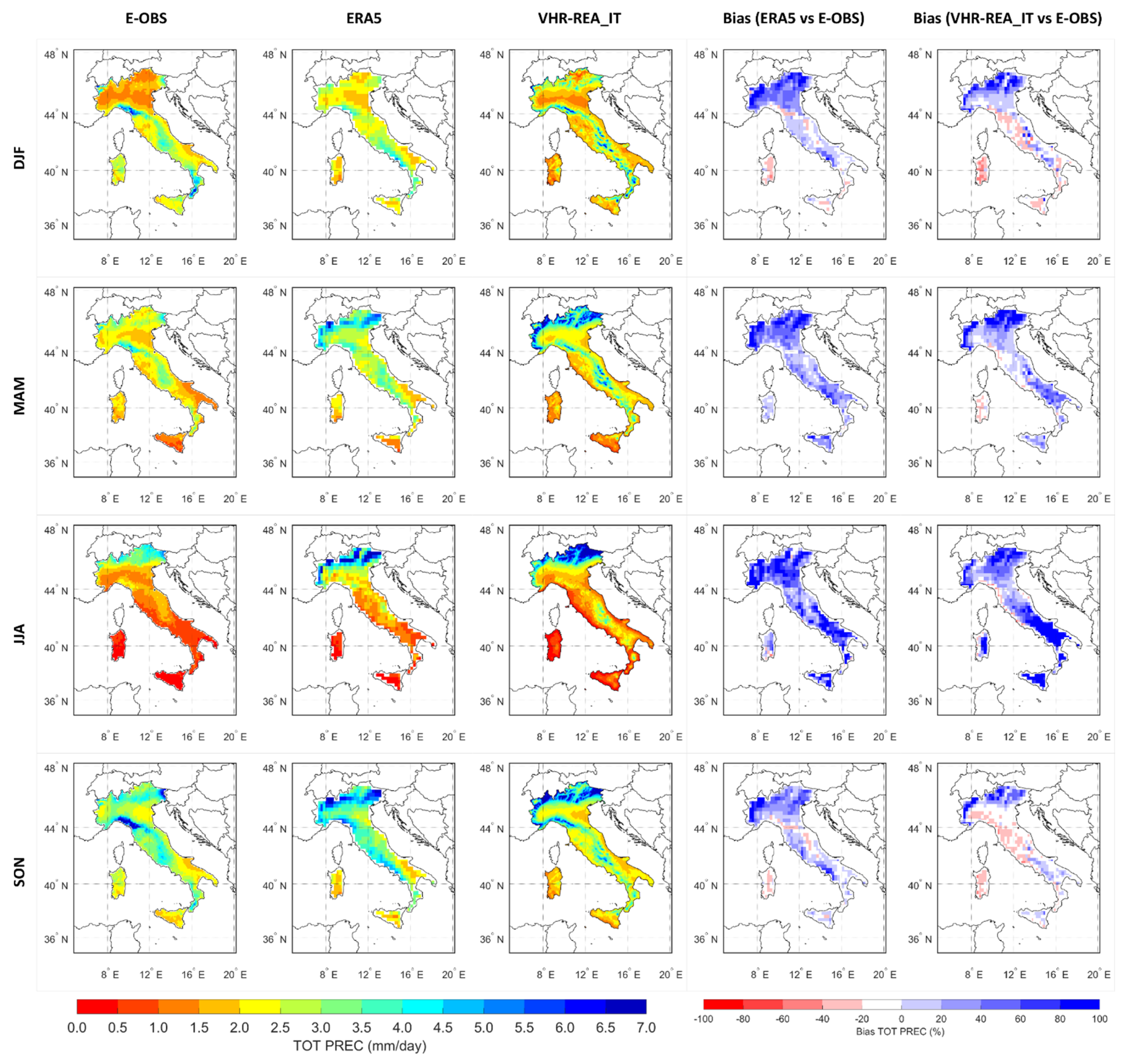
3.1.2. Precipitation

Figure 3 depicts the seasonal spatial distribution of daily precipitation computed for the period 1989–2020 with E-OBS, ERA5, and VHR-REA_IT (the first three columns) on their relative native grids. The same Figure also shows the seasonal spatial distribution of 2 m temperature bias with ERA5 and VHR-REA_IT (the last two columns) assuming E-OBS as a reference. In this case, no correction for elevation has been applied.

Additionally, in this case, to support the validation activity and provide a more comprehensive overview, a summary of results for different areas is reported in

Table 7. Seasonal mean precipitation analysis for the period 1989–2020 provided by E-OBS, ERA5, and VHR-REA_IT. Data are aggregated over Italy and consider the five subareas identified in Figure 1b. For E-OBS, reference values are reported in italic and bold (units = mm/day); for ERA5 and VHR-REA_IT, percent bias (100 * (mod–obs)/obs) and ratio between the standard deviation (σ_mod/σ_obs) are reported. The colors are used to classify differences.

		Bias (%)				σmod/σobs
		DJF	MAM	JJA	SON	DJF	MAM	JJA	SON
Italy	E-OBS	2.27	2.15	1.44	3.02	0.88	0.70	1.09	0.97
	ERA5	12%	33%	50%	17%	0.7	1.5	1.7	1.3
	VHR-REA_IT	0%	24%	42%	−2%	1.1	1.9	1.6	1.4
Northwest Italy	E-OBS	1.91	2.42	2.15	3.40	0.39	0.22	0.18	0.37
	ERA5	30%	51%	70%	31%	0.5	1.4	2.9	1.2
	VHR-REA_IT	29%	51%	42%	22%	0.7	1.6	1.5	0.9
Northeast Italy	E-OBS	1.78	2.37	2.52	3.27	0.38	0.26	0.21	0.50
	ERA5	30%	39%	42%	20%	0.6	1.2	3.1	0.9
	VHR-REA_IT	27%	44%	43%	9%	1.1	1.5	2.0	0.9
Central Italy	E-OBS	2.97	2.56	1.24	3.86	0.24	0.16	0.08	0.27
	ERA5	1%	11%	16%	3%	0.8	1.2	1.8	1.0
	VHR-REA_IT	−15%	−4%	11%	−24%	1.1	1.6	2.7	0.7
South Italy	E-OBS	3.01	2.06	0.77	2.83	0.30	0.17	0.09	0.19
	ERA5	−1%	23%	61%	6%	0.9	1.2	1.9	2.0
	VHR-REA_IT	−9%	17%	86%	−9%	1.3	2.0	3.0	1.5
Insular Italy	E-OBS	2.39	1.47	0.33	2.21	0.12	0.09	0.02	0.08
	ERA5	−10%	15%	29%	−5%	1.0	1.2	3.7	1.8
	VHR-REA_IT	−28%	−12%	42%	−22%	2.5	1.7	6.2	2.2
Bias (%)
σmod/σobs

.

Mean precipitation observations are in general reduced during summer (1.44 mm/day) and relevant during autumn (3.02 mm/day). By looking at Table 7, these values are different in the various areas; specifically, the northern part also exhibits high precipitation during summer while the southern part, as well as the insular area, are rather dry. In comparison with observations, ERA5 tends to increase precipitation across Italy, especially during spring and summer; conversely, the spatial refinement of ERA5 at 2.2 km reduces this wet bias providing values in line with observations, with some exceptions in central, southern, and insular Italy. It is of interest to show how VHR-REA_IT increases summer precipitation against ERA as expected for CP models excepting for Northwest Italy and Central Italy. This is evident, especially in Southern Italy (bias = +86%). Moreover, in terms of spatial variability, the ratio between the standard deviation of RCM data and observations increases, moving from ERA5 to VHR-REA_IT as the refinement of spatial resolution reduces the smoothing of precipitation.

3.1.3. Climate Indicators Evaluation

This section provides an overview about extremes considering climate indicators listed in Table 4 and Table 5. Specifically, these indicators are computed with E-OBS, ERA5, and VHR-REA_IT for each grid cell considering datasets in their native resolution and then aggregated at different spatial units (i.e., over Italy and for the five subareas reported in Figure 1b). The results are reported in

Table 8. List of considered indicators related to temperature.

		ID (Days/Year)	SU (Days/Year)	FD (Days/Year)	TR (Days/Year)	TXx (°C)	90p tmax (°C)	10p tmin (°C)	TNn (°C)
Italy	E-OBS	8	89	41	25	33.6	28.2	1.1	−4.9
	ERA5	10	75	42	32	32.4	27.3	1.0	−5.5
	VHR-REA_IT	12	106	34	54	36.6	30.5	1.7	−4.9
Northwest Italy	E-OBS	21	59	90	7	30.1	25.3	−3.3	−9.6
	ERA5	33	39	99	11	28.6	23.8	−4.8	−12.5
	VHR-REA_IT	35	71	79	35	32.4	27.1	−2.6	−9.3
Northeast Italy	E-OBS	20	72	91	11	31.7	26.5	−3.5	−10.3
	ERA5	24	57	86	20	30.9	25.7	−3.8	−11.4
	VHR-REA_IT	27	84	69	43	34.3	28.7	−2.2	−9.1
Central Italy	E-OBS	2	94	31	13	34.4	29.4	0.9	−5.2
	ERA5	1	75	29	22	32.4	27.9	1.5	−5.1
	VHR-REA_IT	4	110	23	49	37.0	31.5	1.8	−5.3
South Italy	E-OBS	1	96	20	29	34.9	29.3	2.5	−3.3
	ERA5	1	79	21	36	33.0	27.9	2.9	−3.5
	VHR-REA_IT	4	110	18	60	37.5	31.2	3.0	−3.8
Insular Italy	E-OBS	0	108	1	45	34.9	29.6	5.7	0.8
	ERA5	0	102	5	52	34.5	29.3	5.7	0.8
	VHR-REA_IT	0	126	4	73	38.6	31.9	6.0	0.1

for indicators derived from temperature and

Table 9. List of considered indicators related to precipitation.

		CDD (Days/Year)	CWD (Days/Year)	Rx1day (mm/Day)	Rx5day (mm/5 Days)	90p (mm/Day)	99p (mm/Day)	R10 (Days/Year)	R20 (Days/Year)
Italy	E-OBS	47	8	47.3	93.5	19.4	44.0	26	8
	ERA5	32	10	48.7	94.6	16.9	40.5	28	9
	VHR-REA_IT	42	7	64.0	106.4	22.7	56.9	27	11
Northwest Italy	E-OBS	34	8	53.5	109.8	21.2	48.8	30	10
	ERA5	21	12	64.8	132.1	20.5	51.2	38	15
	VHR-REA_IT	30	8	77.1	144.7	27.0	65.5	37	17
Northeast Italy	E-OBS	32	8	48.3	98.1	20.2	43.3	30	10
	ERA5	22	11	53.7	106.0	19.0	43.2	37	13
	VHR-REA_IT	28	8	64.3	115.2	24.0	54.7	38	16
Central Italy	E-OBS	36	8	56.7	110.9	22.7	50.7	33	12
	ERA5	25	10	50.8	99.4	18.8	42.4	33	11
	VHR-REA_IT	37	6	60.1	98.7	22.5	52.9	27	11
South Italy	E-OBS	45	8	46.3	92.8	18.9	43.3	26	8
	ERA5	29	9	48.3	93.7	16.1	39.6	26	8
	VHR-REA_IT	38	6	68.9	110.4	22.8	60.0	25	10
Insular Italy	E-OBS	71	7	42.9	79.3	17.7	41.5	19	5
	ERA5	52	7	37.8	68.9	13.9	33.9	16	4
	VHR-REA_IT	67	5	53.0	79.5	19.4	52.3	14	5

for indicators derived from precipitation.

In general, the analysis of extreme climate indicators reflects the tendency of VHR-REA_IT to amplify climate dynamics due to the spatial resolution refinement.

4. User Notes

The dataset VHR-REA_IT aims to provide a set of unprecedented high-quality and very high-resolution historical climate data. It allows users to assess recent trends in average and extreme climatic conditions that led to numerous cascading hazards over the land surface and connected sectors. Typical use of this dataset is research and downstream services, e.g., for decision support systems in different sectors highly affected by changes in climate trends, variability, and extreme events, as in the case of Italy. For example, starting from the time series of climate data, process-based hydrological modelling can be applied to simulate water cycle components, like evapotranspiration, soil moisture, and runoff up to discharge, and to produce indicators of meteorological–hydrological–agricultural drought attributes, i.e., frequency, magnitude, duration, and timing. The same time series can drive crop or forest growth models assessing vegetation productivity through reproduction of carbon, water, and energy exchanges, as well as feed fire hazard indicators and fire behavior simulations. Last but not least, diurnal, seasonal to interannual variability of extreme conditions can help in assessing changes to dangerous conditions for people and animals, allowing us to discriminate between rural and urban environments thanks to the high spatial resolution implemented.

The VHR-REA_IT dataset features some limitations that must be properly considered for correct use. Although it is obtained by dynamically downscaling a reanalysis (i.e., ERA5), some biases may be noticed due to the absence of a data assimilation procedure, which, considering the resolution of this new dataset, is hard to include over all domains with the same characteristic.

In this sense, it is also important to stress how the use of an urban parameterization such as TERRA-URB correctly leads to an increasing of temperature over urban centers. Such an increase is hard to detect by ERA5 reanalysis or E-OBS observations due to their resolution (at least five times lower for E-OBS and 15 times lower for ERA5). It could be evaluated against observations provided by urban meteorological stations. However, these measurements are hard to retrieve as synoptic stations are often used.

To sum up, some biases may be encountered; they should be evaluated with punctual observations and appropriately removed through bias correction procedures to correctly feed impact models.

References

1. Kendon, E.J.; Prein, A.F.; Senior, C.A.; Stirling, A. Challenges and outlook for convection-permitting climate modelling. Philos. Trans. R. Soc. 2021, 379, 20190547. [Google Scholar] [CrossRef] [PubMed]
2. Ban, N.; Schmidli, J.; Schär, C. Evaluation of the new convective-resolving regional climate modelling approach in decade-long simulations. J. Geophys. Res. Atmos. 2014, 119, 7889–7907. [Google Scholar] [CrossRef]
3. Berthou, S.; Kendon, E.J.; Chan, S.C.; Ban, N.; Leutwyler, D.; Schär, C.; Fosser, G. Pan-European climate at convec-tion-permitting scale: A model intercomparison study. Clim. Dyn. 2018, 5, 1–25. [Google Scholar] [CrossRef] [Green Version]
4. Coppola, E.; Sobolowski, S.; Pichelli, E.; Raffaele, F.; Ahrens, B.; Anders, I.; Ban, N.; Bastin, S.; Belda, M.; Belušić, D.; et al. A first-of-its-kind multi-model convection permitting ensemble for investigating convective phenomena over Europe and the Mediterranean. Clim. Dyn. 2020, 55, 3–34. [Google Scholar] [CrossRef]
5. Fumière, Q.; Déqué, M.; Nuissier, O.; Somot, S.; Alias, A.; Caillaud, C.; Laurantin, O.; Seity, Y. Extreme rainfall in Mediterra-nean France during the fall: Added-value of the CNRM-AROME convection permitting regional climate model. Clim. Dyn. 2020, 55, 77–91. [Google Scholar] [CrossRef] [Green Version]
6. Fosser, G.; Khodayar, S.; Berg, P. Benefit of convection permitting climate model simulations in the representation of convective precipitation. Clim. Dyn. 2015, 44, 45–60. [Google Scholar] [CrossRef] [Green Version]
7. Prein, A.F.; Langhans, W.; Fosser, G.; Ferrone, A.; Ban, N.; Goergen, K.; Keller, M.; Toelle, M.; Gutjahr, O.; Feser, F.; et al. A review on regional convection-permitting climate modeling: Demonstrations, prospects, and challenges. Rev. Geophys. 2015, 53, 323–361. [Google Scholar] [CrossRef] [Green Version]
8. Piazza, M.; Prein, A.F.; Truhetz, H.; Csaki, A. On the sensitivity of precipitation in convection-permitting climate simulations in the Eastern Alpine region. Meteorol. Z. 2019, 28, 323–346. [Google Scholar] [CrossRef]
9. Adinolfi, M.; Raffa, M.; Reder, A.; Mercogliano, P. Evaluation and Expected Changes of Summer Precipitation at Convection Permitting Scale with COSMO-CLM over Alpine Space. Atmosphere 2020, 12, 54. [Google Scholar] [CrossRef]
10. Raffa, M.; Reder, A.; Adinolfi, M.; Mercogliano, P. A Comparison between One-Step and Two-Step Nesting Strategy in the Dynamical Downscaling of Regional Climate Model COSMO-CLM at 2.2 km Driven by ERA5 Reanalysis. Atmosphere 2021, 12, 260. [Google Scholar] [CrossRef]
11. Ban, N.; Caillaud, C.; Coppola, E.; Pichelli, E.; Sobolowski, S.; Adinolfi, M.; Ahrens, B.; Alias, A.; Anders, I.; Bastin, S.; et al. The first multi-model ensemble of regional climate simulations at kilometer-scale resolution, part I: Evaluation of precipitation. Clim. Dyn. 2021, 57, 275–302. [Google Scholar] [CrossRef]
12. Fowler, H.J.; Wasko, C.; Prein, A.F. Intensification of short-duration rainfall extremes and implications for flood risk: Current state of the art and future directions. Philos. Trans. R. Soc. A: Math. Phys. Eng. Sci. 2021, 379, 20190541. [Google Scholar] [CrossRef]
13. Reder, A.; Raffa, M.; Montesarchio, M.; Mercogliano, P. Performance evaluation of regional climate model simulations at different spatial and temporal scales over the complex orography area of the Alpine region. Nat. Hazards 2020, 102, 151–177. [Google Scholar] [CrossRef]
14. Taylor, C.; Birch, C.E.; Parker, D.; Dixon, N.; Guichard, F.; Nikulin, G.; Lister, G.M.S. Modeling soil moisture-precipitation feedback in the Sahel: Importance of spatial scale versus convective parameterization. Geophys. Res. Lett. 2013, 40, 6213–6218. [Google Scholar] [CrossRef] [Green Version]
15. Trusilova, K.; Früh, B.; Brienen, S.; Walter, A.; Masson, V.; Pigeon, G.; Becker, P. Implementation of an Urban Parameterization Scheme into the Regional Climate Model COSMO-CLM. J. Appl. Meteorol. Climatol. 2013, 52, 2296–2311. [Google Scholar] [CrossRef]
16. Hersbach, H.; Bell, B.; Berrisford, P.; Hirahara, S.; Horanyi, A.; Muñoz-Sabater, J.; Nicolas, J.; Peubey, C.; Radu, R.; Schepers, D.; et al. The ERA5 global reanalysis. Q. J. R. Meteorol. Soc. 2020, 146, 1999–2049. [Google Scholar] [CrossRef]
17. Buontempo, C.; Hutjes, R.; Beavis, P.; Berckmans, J.; Cagnazzo, C.; Vamborg, F.; Thépaut, J.-N.; Bergeron, C.; Almond, S.; Amici, A.; et al. Fostering the development of climate services through Copernicus Climate Change Service (C3S) for agriculture applications. Weather. Clim. Extremes 2020, 27, 100226. [Google Scholar] [CrossRef]
18. UCAR/Unidata Program Center. Unidata, Network Common Data Form (NetCDF), V4.8.0; UCAR/Unidata Program Center: Boulder, CO, USA, 2019. [Google Scholar]
19. Cornes, R.C.; Van Der Schrier, G.; Besselaar, E.V.D.; Jones, P.D. An Ensemble Version of the E-OBS Temperature and Precipitation Data Sets. J. Geophys. Res. Atmos. 2018, 123, 9391–9409. [Google Scholar] [CrossRef] [Green Version]
20. Rockel, B.; Will, A.; Hense, A. The Regional Climate Model COSMO-CLM (CCLM). Meteorol. Z. 2008, 17, 347–348. [Google Scholar] [CrossRef]
21. Wouters, H.; Demuzere, M.; Blahak, U.; Fortuniak, K.; Maiheu, B.; Camps, J.; Tielemans, D.; van Lipzig, N.P.M. The efficient urban canopy dependency parametrization (SURY) v1.0 for atmospheric modelling: Description and application with the COSMO-CLM model for a Belgian summer. Geosci. Model. Dev. 2016, 9, 3027–3054. [Google Scholar] [CrossRef] [Green Version]
22. Ritter, B.; Geleyn, J.F. A comprehensive radiation scheme for numerical weather prediction models with potential applications in climate simulations. Mon. Weather Rev. 1992, 120, 303–325. [Google Scholar] [CrossRef] [Green Version]
23. Tiedtke, M. A comprehensive mass flux scheme for cumulus parameterization in large-scale models. Mon. Weather Rev. 1989, 117, 1779–1800. [Google Scholar] [CrossRef] [Green Version]
24. Doms, G.; Forstner, J.; Heise, E.; Herzog, H.J.; Mironov, D.; Raschendorfer, T.; Reinhardt, T.; Ritter, B.; Schrodin, R.; Schulz, J.P.; et al. A Description of the Non-Hydrostatic Regional COSMO Model. Part-II: Physical Parameterization. 2011. Available online: https://klimanavigator.eu/imperia/md/content/csc/klimanavigator/cosmophysparamtr.pdf (accessed on 23 December 2020).
25. Baldauf, M.; Schulz, J.P. Prognostic precipitation in the lokal modell (LM) of DWD. COSMO Newsletter No. 4.; Deutscher Wetterdienst: Offenbach am Main, Germany, 2004; pp. 177–180. [Google Scholar]
26. Bartholomé, E.; Belward, A.S. GLC2000: A new approach to global land cover mapping from Earth observation data. Int. J. Remote. Sens. 2005, 26, 1959–1977. [Google Scholar] [CrossRef]
27. Mellor, G.L.; Yamada, T. A hierarchy of turbulence closure models for planetary boundary layers. J. Atmos. Sci. 1974, 31, 1791–1806. [Google Scholar] [CrossRef] [Green Version]
28. Giorgi, F.; Gutowski, W.J. Regional Dynamical Downscaling and the CORDEX Initiative. Annu. Rev. Environ. Resour. 2015, 40, 467–490. [Google Scholar] [CrossRef]
29. Jacob, D.; Petersen, J.; Eggert, B.; Alias, A.; Christensen, O.B.; Bouwer, L.M.; Braun, A.; Colette, A.; Déqué, M.; Georgievski, G.; et al. EURO-CORDEX: New high-resolution climate change projections for European impact research. Reg. Environ. Chang. 2014, 14, 563–578. [Google Scholar] [CrossRef]
30. Padulano, R.; Rianna, G.; Santini, M. Datasets and approaches for the estimation of rainfall erosivity over Italy: A comprehensive comparison study and a new method. J. Hydrol. Reg. Stud. 2021, 34, 100788. [Google Scholar] [CrossRef]
31. Haylock, M.R.; Hofstra, N.; Tank, A.K.; Klok, E.J.; Jones, P.; New, M. A European daily high-resolution gridded data set of surface temperature and precipitation for 1950–2006. J. Geophys. Res. Space Phys. 2008, 113. [Google Scholar] [CrossRef] [Green Version]
32. Prein, A.F.; Gobiet, A. Impacts of uncertainties in European gridded precipitation observations on regional climate analysis. Int. J. Clim. 2017, 37, 305–327. [Google Scholar] [CrossRef]
33. Isotta, F.A.; Frei, C.; Weilguni, V.; Tadić, M.P.; Lassègues, P.; Rudolf, B.; Pavan, V.; Cacciamani, C.; Antolini, G.; Ratto, S.M.; et al. The climate of daily precipitation in the Alps: Development and analysis of a high-resolution grid dataset from pan-Alpine rain-gauge data. Int. J. Clim. 2013, 34, 1657–1675. [Google Scholar] [CrossRef]
Figure 1. (a) Surface height (m a.s.l.); (b) area considered for technical validation, defined according to the first level of Nomenclature of Territorial Units for Statistics (NUTS 1) for Italy.
Data 06 00088 g001
Figure 2. The first three columns: Seasonal (in row) spatial distribution of 2 m temperature for the period 1989–2020 provided by E-OBS, ERA5, and VHR-REA_IT (in column); the last two columns: Seasonal (in row) spatial distribution of 2 m temperature bias for the period 1989–2020 provided by ERA5 and VHR-REA_IT (in column) assuming E-OBS as a reference.
Data 06 00088 g002
Figure 3. The first three columns: Seasonal (in row) spatial distribution of daily precipitation for the period 1989–2020 provided by E-OBS, ERA5, and VHR-REA_IT (in column); the last two columns: Seasonal (in row) spatial distribution of daily precipitation bias for the period 1989–2020 provided by ERA5 and VHR-REA_IT (in column), assuming E-OBS as a reference.
Data 06 00088 g003