1. Summary
The dataset is a collection of seismic envelopes computed from the seismograms of 280 earthquakes occurred in the Gargano area (Southern Italy) and recorded by both the OTRIONS (OT) and INGV (IV) seismic networks. The selected earthquakes belong to two bulletins: the first refers to earthquakes that occurred from June to September 2013; the second refers to earthquakes that occurred from July 2015 to August 2018. All of these earthquakes belong to a seismic database that was recently released and described [
1,
2,
3] together with the seismic bulletins, station locations, velocity model [
3], and seismograms.
Seismic attenuation estimates are calculated from the decay of coda waves that constitute the end of the seismic recording for local and regional events. The coda waves start after the S waves and are composed of incoherent waves scattered by inhomogeneities. The amplitude of coda waves is thought to decrease because of the seismic attenuation (both intrinsic and scattering) and because of the geometrical spreading of the wave front. Aki and Chouet [
4] showed that, assuming that coda waves are single-scattered S waves, at short source–receiver distances, the coda amplitude decay
is given by:
that is a linearly decreasing function of the time
elapsed from the origin time of the earthquake for a given central frequency
. Therefore,
can be estimated by the slope of the linear regression in Equation (1) in a selected time window called a lapse time window
. On the seismogram
, the seismic coda decay
can be evaluated by the seismic envelope calculated using the Hilbert transform
, as follows:
The dependence of
on
is obtained by band-pass filtering the signal
around
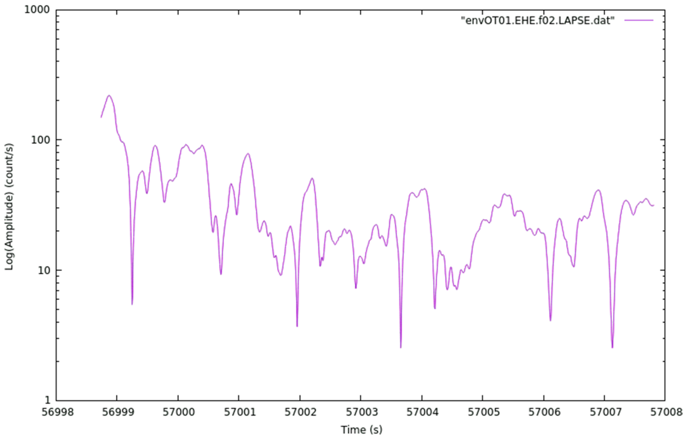
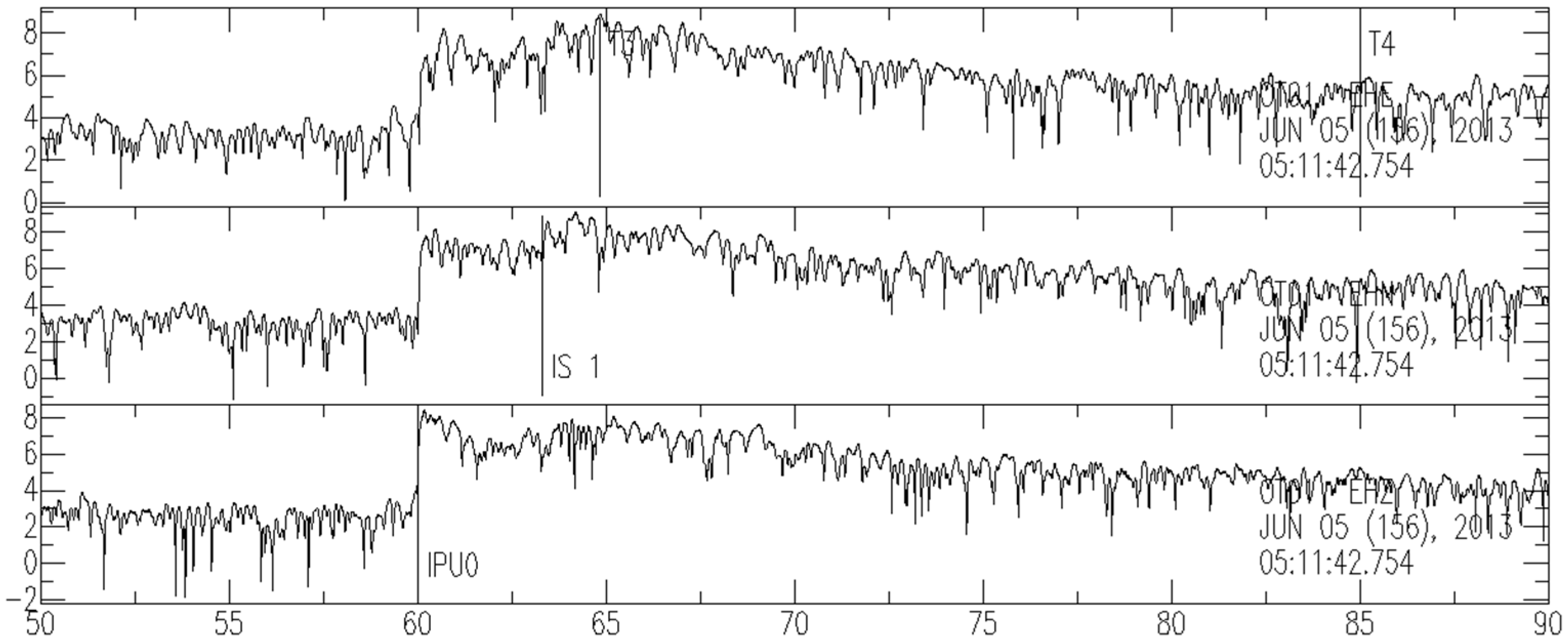
In this work, we release the seismic envelopes
cut between the time T3, marked on the seismogram after the S-wave arrival time, until time T4, marked on the seismogram before an energy bump or an irregularity of the coda decay or when the coda waves are indistinguishable from the noise content. All released envelopes are band-pass filtered with a two-pole Butterworth filter, considering 11 values of
Hz and a band-width
, following Bianco et al. [
5]. Times T3 and T4 were manually marked on seismogram envelopes filtered with central frequency
= 6 Hz and band-width [4.2; 8.5] Hz.
The first dataset of envelopes (
http://0-dx-doi-org.brum.beds.ac.uk/10.17632/w9hsj2whzm.1#folder-7a917d26-6be4-4014-8103-a8760541264a, accessed on 5 September 2021), which consists of the recordings of the period from June to September 2013, was already used for the first 2D
study [
6] of the Gargano Promontory (Southern Italy). It consists of the recordings of 89 microearthquakes, with magnitudes ranging between 0.8 and 1.8, that were recently used to study the Gargano stress field [
7] and the rheology of the Gargano crust [
8].
The manual work behind the time markers recognizing procedure is very expensive in terms of time costs. Nevertheless, we think that with this manual time marking procedure we obtained a very robust dataset of time envelopes with respect to an automatic time cut of seismic recordings. The released datasets of seismic envelopes can be very useful for seismological studies of intrinsic and scattering attenuation of Southern Italy, the Adriatic Sea, and other surrounding regions at different time lapse windows .
3. Methods
The two datasets described in
Section 2.1 and
Section 2.2 were collected by using the SAC (Seismic Analysis Code) software [
11,
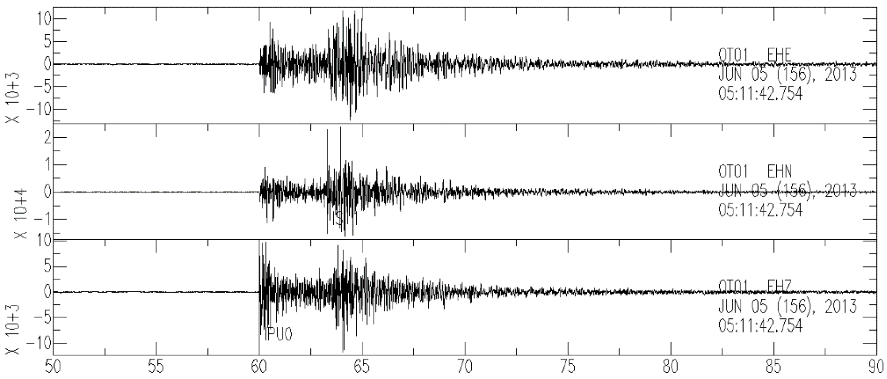
12]. Starting from the original seismogram in
Figure 3, a filtering procedure is applied by using a two-pole Butterworth filter considering a central frequency
Hz and a band-width
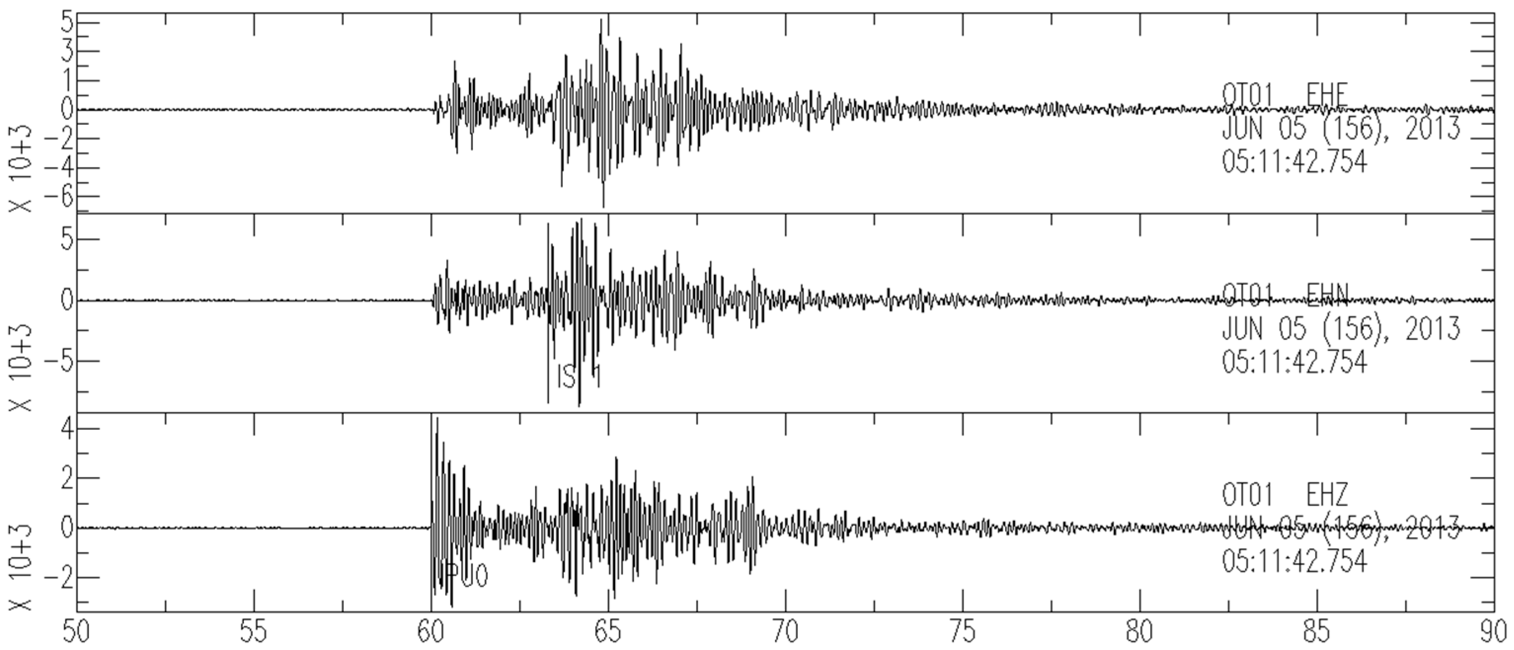
, thereby obtaining 11 new files for each seismogram component (for an example, see
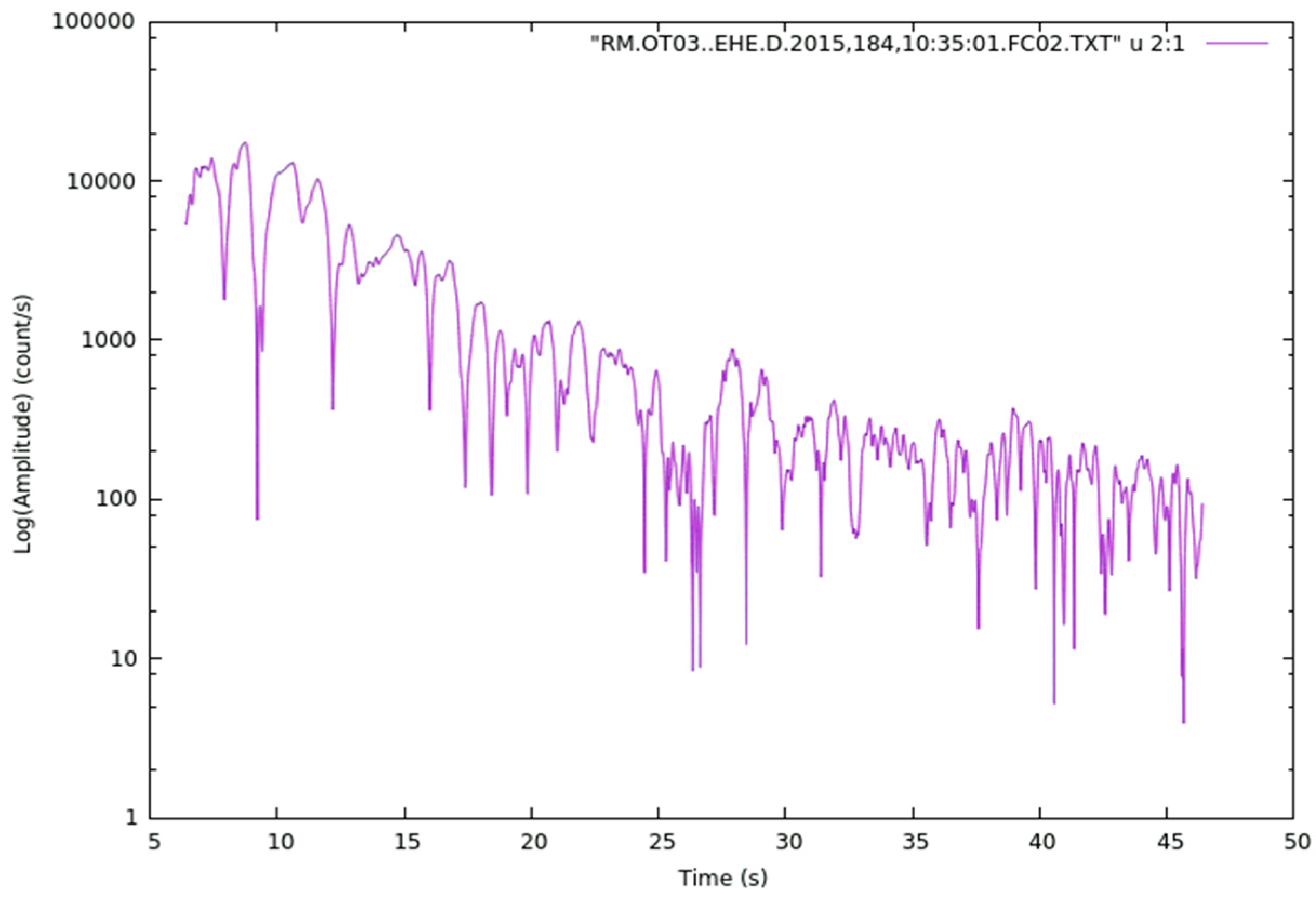
Figure 4). To each filtered seismogram, the SAC function “ENVELOPE” was applied, which computes the envelope function using a Hilbert transform using Equation (2) (for an example, see
Figure 5). The released datasets are the envelopes cut inside the [T3, T4] time window, as shown in
Figure 1. To these files, a linear regression in Equation (1) was applied to retrieve the
value at each frequency [
6]. A discussion about errors and uncertainties can be found in [
9].


