
An Estimated-Travel-Time Data Scraping and Analysis Framework for Time-Dependent Route Planning †


Department of Computer Science, Faculty of Information and Communication Technology, Universiti Tunku Abdul Rahman, Kampar Campus, Perak 31900, Malaysia
*
Author to whom correspondence should be addressed.
†
This paper is an extended version of “Tee, H.L.; Liew, S.Y.; Wong, C.S.; Ooi, B.Y. Cost-effective scraping and processing of real-time traffic data for route planning. In Proceedings of the 2021 International Conference on Computer & Information Sciences (ICCOINS), Kuching, Malaysia, 13–15 July 2021; IEEE: Piscataway, NJ, USA, 2021; pp. 264–269”.
Data 2022, 7(5), 54; https://0-doi-org.brum.beds.ac.uk/10.3390/data7050054
Submission received: 25 November 2021
/
Revised: 15 February 2022
/
Accepted: 19 April 2022
/
Published: 27 April 2022
(This article belongs to the Special Issue Knowledge Extraction from Data Using Machine Learning)
Abstract
:Generally, a courier company needs to employ a fleet of vehicles to travel through a number of locations in order to provide efficient parcel delivery services. The route planning of these vehicles can be formulated as a vehicle routing problem (VRP). Most existing VRP algorithms assume that the traveling durations between locations are time invariant; thus, they normally use only a set of estimated travel times (ETTs) to plan the vehicles’ routes; however, this is not realistic because the traffic pattern in a city varies over time. One solution to tackle the problem is to use different sets of ETTs for route planning in different time periods, and these data are collectively called the time-dependent estimated travel times (TD-ETTs). This paper focuses on a low-cost and robust solution to effectively scrape, process, clean, and analyze the TD-ETT data from free web-mapping services in order to gain the knowledge of the traffic pattern in a city in different time periods. To achieve the abovementioned goal, our proposed framework contains four phases, namely, (i) Full Data Scraping, (ii) Data Pre-Processing and Analysis, (iii) Fast Data Scraping, and (iv) Data Patching and Maintenance. In our experiment, we used the above framework to obtain the TD-ETT data across 68 locations in Penang, Malaysia, for six months. We then fed the data to a VRP algorithm for evaluation. We found that the performance of our low-cost approach is comparable with that of using the expensive paid data.
1. Introduction
The number of vehicles travelling on the roads in a city varies over time, and the resulting traffic pattern is actually an important factor that logistics companies, such as those providing courier services, need to consider when planning routes for their vehicles. Generally, a courier company owns multiple outlets in a city for senders to submit their parcels. Then, the vehicles of the company have to travel to all the outlets to collect these parcels, send them for sorting, and deliver them to the respective recipients. The travelling routes of the vehicles between the outlets and the sorting center can be formulated as a Vehicle Routing Problem (VRP).
In order to improve the efficiency of parcel collection and delivery services, the courier company needs accurate traffic data in order to plan the routes of the vehicles; however, most of the existing algorithms solve the VRP by assuming that the travelling durations between locations are time invariant, and thus, they normally use only a set of travel input data to plan the vehicles’ routes all of the time. This may not be realistic because the traffic pattern in a city is variable depending on the period of the day, and this causes the travelling duration between two specific locations to change from time to time. In other words, the travel time from a location to another location is actually time dependent. Neglecting the time dependency can introduce significant errors to route planning.
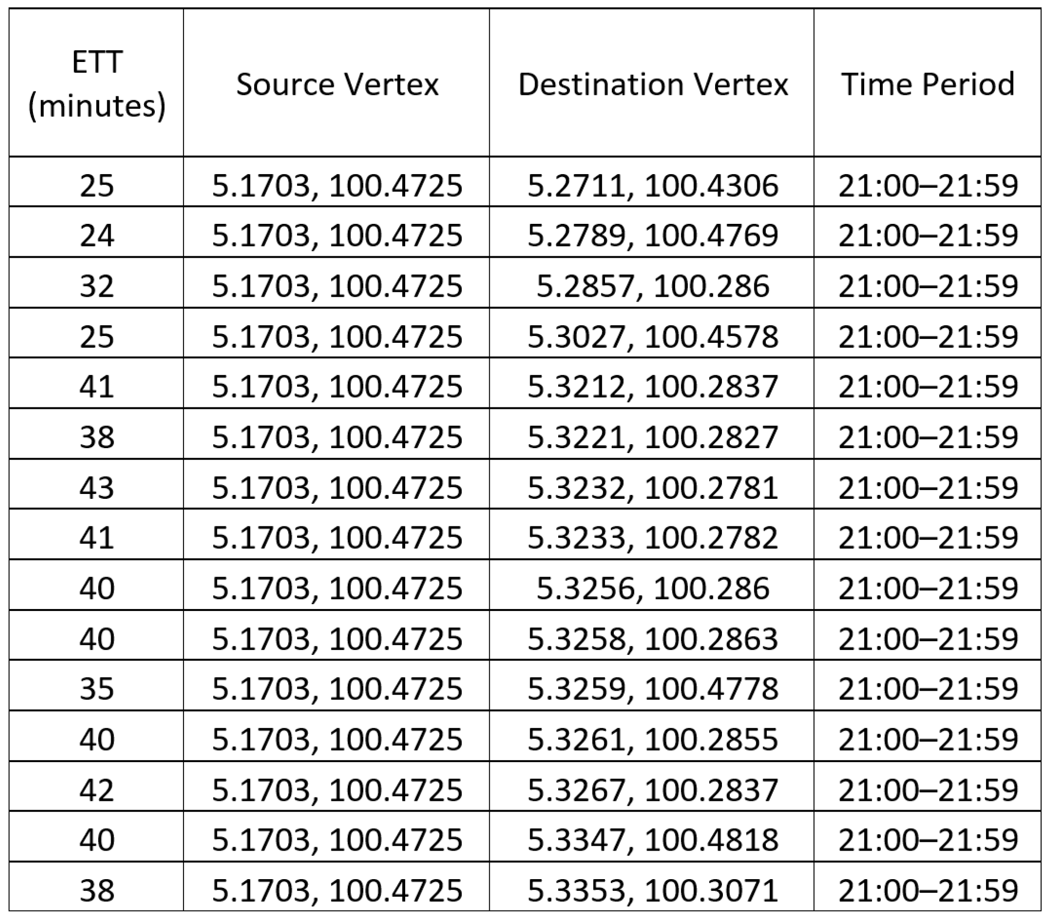
One solution to tackle the problem is to use different sets of estimated travel times (ETTs) for route planning in different time periods. Collectively, these different sets of ETTs are called the time-dependent estimated travel times (TD-ETTs). The TD-ETT is a four-dimensional data set, and each entry includes (1) the estimated travel time from (2) a source vertex to (3) a destination vertex in (4) a particular time period as shown in Figure 1, where the vertices represent the geographical locations denoted by their respective longitude-latitude coordinates in the region.
Such TD-ETT data can actually be bought from the web-mapping companies; however, depending on the number of outlets and the sets of ETT data required, the acquisition of a full set of TD-ETT data is normally very expensive and not affordable to most courier companies.
Other than paying for web-mapping data, the courier company can also install the Global Positioning System (GPS) in their fleet of vehicles and subscribe the relevant services from a GPS service provider [1]. This enables the courier company to keep track of the travel times spent by the vehicles to travel between their outlets accurately; however, it is impossible for the fleet of vehicles to collect all TD-ETT data between outlets because the size of the fleet is limited and thus not all sets of traveling paths in different time periods can be covered.
Another possible solution is that the courier company can capture the past traffic data, so that it can learn and analyze the past data in order to estimate the future travel times between outlets accurately. With the estimation, the routes for vehicles can be properly planned even before they depart. For this approach, however, sufficient data must be collected first so that they can be pre-processed, cleaned, and analyzed in order to produce accurate TD-ETT values for the route optimization process.
In this research, we study a low-cost and robust framework that is able to scrape, process, clean, and analyze the TD-ETT data for a set of pre-determined outlet locations in a city. The proposed framework is at a low cost because the data collection is done through scraping the data from the free web-mapping services; it is also robust because the data maintenance strategy is derived from the processing and analysis of the scraped data.
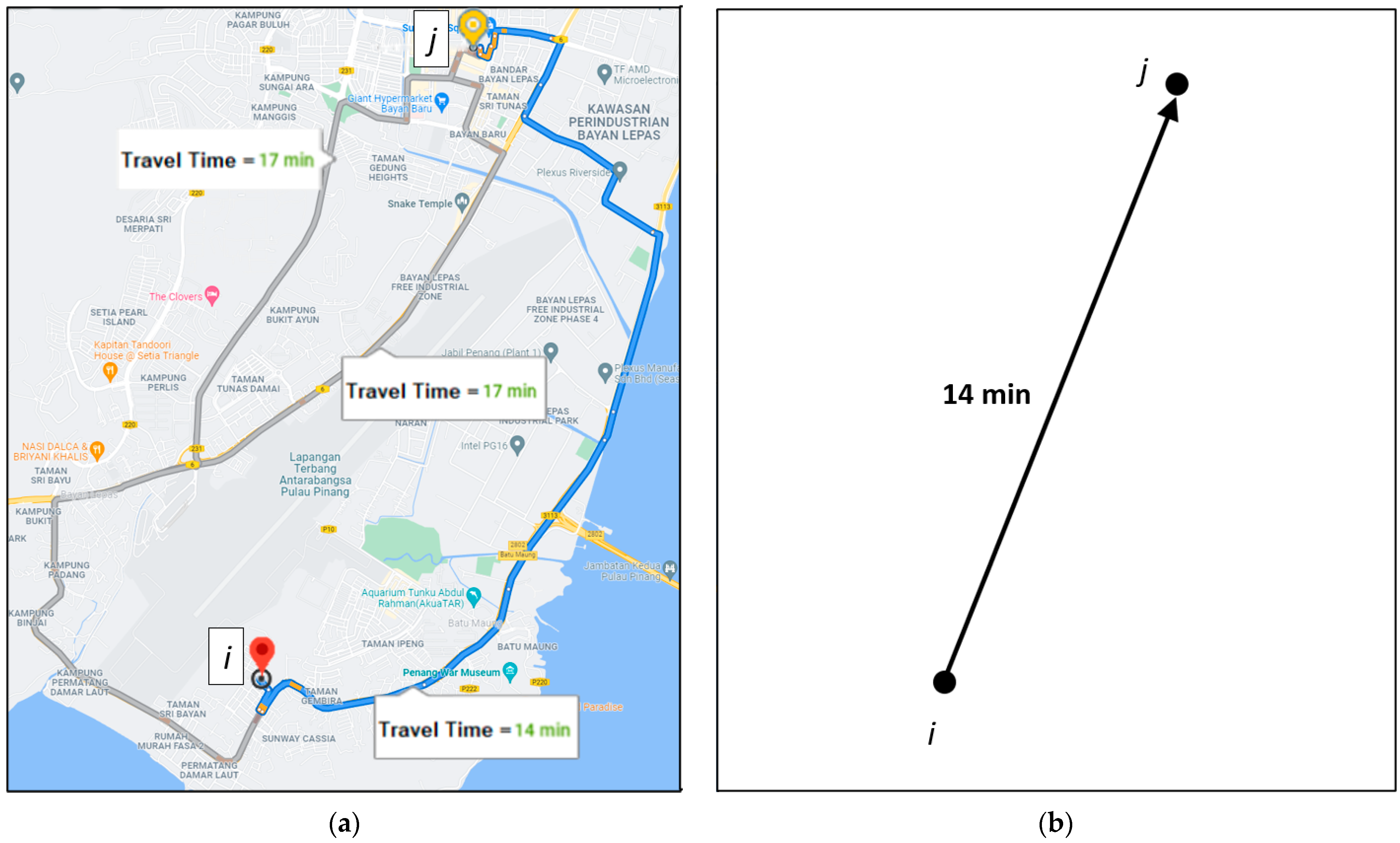
In general, the points of interest in a geographical region can be represented by a set of vertices, V, in a directed graph, G. The arc from vertex i to vertex j exists if, and only if, there is a possible route from point i to point j in the real map. In a city with a good road network, the representing graph G should be a fully connected directed graph because there must be at least a route from any point of interest to another. Note that the route from i to j may not be the same as the route from j to i, depending on the real road condition in the geographical region. For a particular time period, we can further label each arc in G with the ETT of the best route as the weight of the arc. An example of traveling from one point to another on a geographical map and its representation in a directed graph is shown in Figure 2.
Through our experiment, we found that the ETT data provided by the web-mapping company may not be always optimum, regardless of whether the data are paid or free of charge. It is because the ETT data returned from the web-mapping services are highly dependent on the route selections of the backend routing algorithm. Owing to the limitation of the backend routing algorithm, not only that the selected routes may be non-optimum, but there can also be illogicality among some routes. For instance, the ETT from vertex i to vertex j is larger than the sum of the ETTs from vertex i to vertex k and then from vertex k to vertex j, which violates the triangle inequality principle. Such illogicality is actually not uncommon with the ETTs obtained from the web-mapping services. If we directly use the ETTs returned from the web-mapping services as the weights of the arcs, then the existence of the illogicalities will affect the effectiveness and correctness of the route planning algorithms.
Therefore, a data pre-processing phase is also introduced in our framework to identify and patch the arcs with illogical scraped ETT values in order to improve the correctness of the data. Such a pre-processing phase is also important to the subsequent data scraping process because the arcs that consistently contain illogical scraped ETT values can be removed from being scraped in the future cycle, because even in the absence of the scraped data, the weights can just be patched by alternative routes with better combined ETTs. In doing so, time required to scrape ETT data in a cycle can also be reduced, and thus more cycles can be completed in a given time in order to increase the time-dependent fineness of the data.
To achieve the abovementioned goal, our proposed approach can be divided into four phases, namely, (i) Full Data Scraping, (ii) Data Pre-Processing and Analysis, (iii) Fast Data Scraping, and (iv) Data Patching and Maintenance. Their objectives are described as follows.
In the (i) Full Data Scraping phase, the full set of ETTs in a particular time period will be scraped. It should be noted that since the entire set of ETTs need to be scraped, the interval of the scraping cycle is rather long, and thus the number of cycles is limited. This phase will continue for weeks in order to collect enough ETT data.
In the (ii) Data Pre-Processing and Analysis phase, the illogical ETT values will be identified by applying the inequality principle shown in Theorem 1 in Section 3. If for a particular arc, the illogicality happens frequently up to a certain threshold, the corresponding ETT value can then be safely replaced by the alternative shorter ETT by taking another route with a transit point. Such a relationship will also be learned in this phase.
In the (iii) Fast Data Scraping phase, all the illogical arcs will be removed from the scraping process. This will shorten the scraping cycle and more cycles can be completed in a given time. As a result, the number of ETT data sets in a given time can be increased, and thus more accurate ETT data in the time period can be obtained. This process will continue until there is a need for another full data scraping.
Since the arcs with the consistently illogical scraped ETTs have been removed from the previous phase, the missing ETT values have to be patched before the entire set of TD-ETTs can be fed to the route planning algorithm; therefore, in the (iv) Data Patching and Maintenance phase, the first objective is to patch the missing ETT values with the relationships (equations) learned in phase (ii). Moreover, although we continue to use the reduced graph for data scraping in (iii), after a certain number of cycles, a new round of full data scraping needs to be executed again in order to verify and maintain the data.
The work presented in this paper is actually an extension of our previous work in [2]. In our previous work, we only performed the first phase, (i) Full Data Scraping, and we partially performed the second phase in the proposed framework; however, the entire data cleaning process was not formulated in [2] and the full cycle of the scraping process also takes a long time, which affects the fineness of the collected data.
The novelty of this paper lies in the following three aspects: (1) the overall concept of data cleaning for the practical implementation of VRP algorithms for route planning; (2) the analysis of the full set of TD-ETT data with the aim to reduce the amount of data to be subsequently scraped; (3) a framework that collects TD-ETT data with shortened cycles to get finer data, while maintaining the validity and accuracy of the data. This is done by introducing (ii) Data Pre-Processing and Analysis (full phase), the (iii) Fast Data Scraping phase and the (iv) Data Patching and Maintenance phase. We have also expanded our scope of research to study the relationship between the scraping efficiency and accuracy of data collection. We believe that the outcomes of this study could offer practical insights that could be useful to logistics industry.
In our experiment, we scraped, processed, cleaned, analyzed, and maintained the TD-ETT data across 68 outlets of a courier company in Penang, a state of Malaysia, for six months; we then fed the data produced by our approach to some VRP algorithms, such as the Traveling Salesman Problem algorithm, and found that the performance of our low-cost approach is comparable with that of using the full set of paid data.
The remainder of the paper is organized as follows. Section 2 discusses the related works in the literature. In Section 3, we elaborate the methodology of this research. Experiment setting, results and possible extended works will be presented in Section 4. Finally, the conclusions are discussed in Section 5.
2. Related Work
In traditional route planning approaches, the travelling duration between two points is assumed to be known and fixed prior to the planning stage; however, it is not applicable in real world situations as real traffic varies over time; therefore, the approaches without considering time-dependent traffic conditions will result in poor planning even though the algorithms are robust [3,4,5]. Thus, to generate a more reasonable travel time estimation, past traffic data have to be studied in order to extract the information and find out a realistic estimation for inputs for the route planning algorithms.
2.1. Data Collection
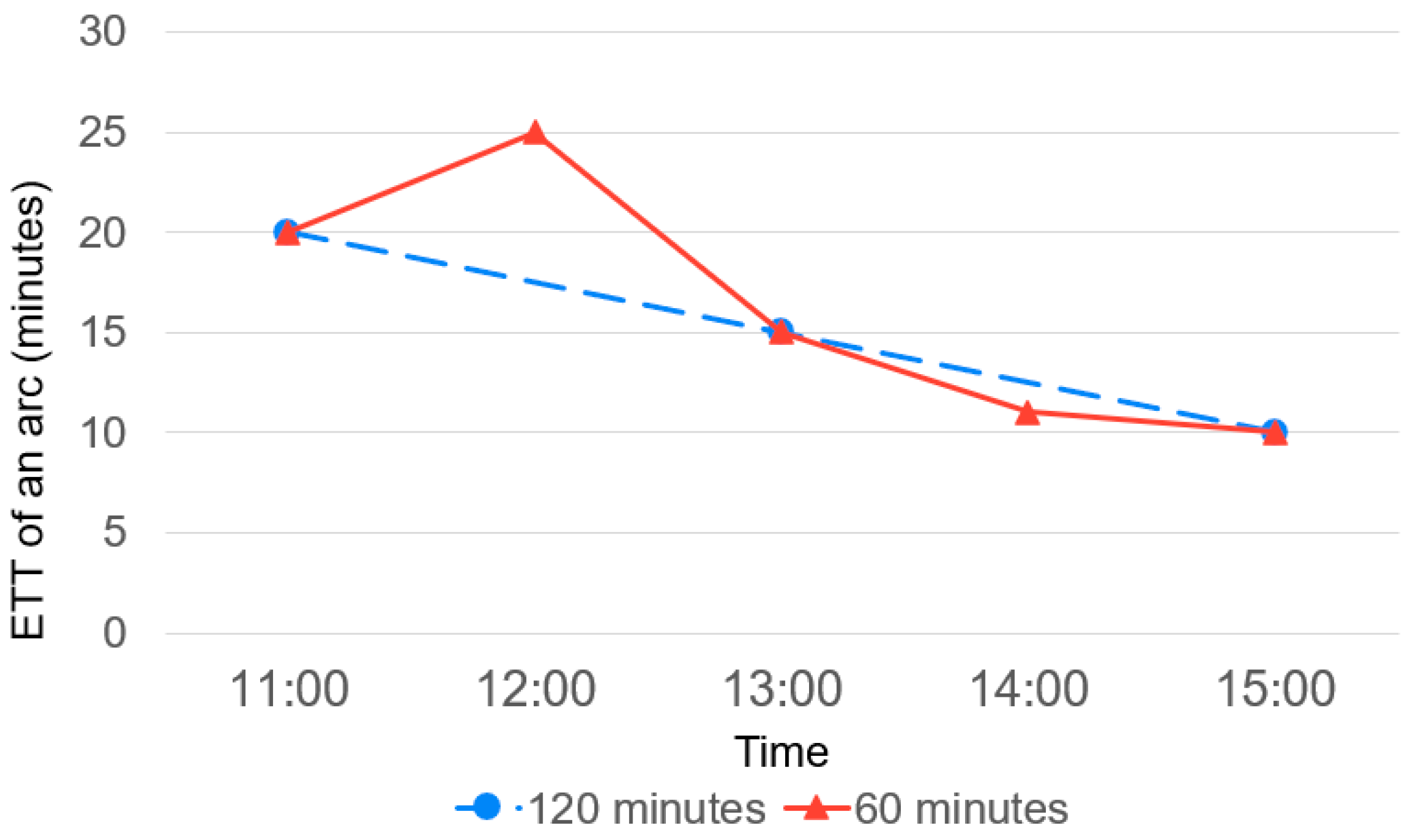
There are a few approaches for data collection on historical traffic data, namely, (i) web scraping, (ii) distance matrix API, and (iii) GPS. To find out the most feasible methods for data collection, these three methods are compared in terms of monetary costs and accuracy as follows. It is crucial to collect the ETT data as frequently as possible to obtain more samples and information about the changes of traffic data. In general, the shorter the interval between two samples, the better the accuracy of ETT for route planning algorithms. An example of benefits to have a faster data collection cycle is shown in Figure 3.
Figure 3 shows the scraped data of the ETTs between two geographical points with two different interval settings, i.e., 60 min and 120 min. For the 120 min scraping interval, interpolation will be needed to make an estimation of the travel time between two scraped samples, and it can be obtained by taking the average value of the two samples; however, this might result in the inaccuracy of data, as shown in Figure 3. In this example, the 120 min scrapping interval fails to capture the peak at 12:00. In general, the shorter the interval, the finer the time-dependent data. In order to increase the accuracy, the fineness of data is therefore an important factor to be considered in any time-dependent data maintenance framework.
The research in [6] considers using GPS to collect actual-time traffic data, and it is highlighted in [6] that GPS traffic data further helps to create dynamic routes with the real-time traffic data input; however, this approach is rather costly. For example, one of the local GPS service providers in Malaysia [7] is charging around USD 17.06 per month to track a vehicle. Assume that there are 50 vehicles of a courier company that employ the GPS service. Choosing the Lite plan costs roughly USD 853 per month. Another issue is, even though the GPS service is more likely to provide a higher accuracy of the travelling duration between two points as it captures the data in real-time as the vehicle travels, the fleet of vehicles will not be able to collect all required traffic data over a geographical area at all possible times because the travelling paths of these vehicles are limited. This results in the incompleteness of data when finding optimal routes in different time periods.
Kim et al. [8] collected past traffic data from Michigan Intelligent Transportation System Center; however, the outcome of route planning using the given past traffic data may not be feasible. This is because the collected data had an age of 5 years when the research was being carried out, and thus the data might not have fully reflected the changes of the road layouts and the increasing number of vehicles on roads. This directly affects the accuracy of route planning with the given data.
Google Maps Distance Matrix API is used by [9] to collect real-time ETT data. According to the pricing reference from Google Developer [10], at the time of writing, it costs USD 0.008 per API call. The pricing is considered costly if the ETT data among many locations is required for the route planning. For instance, in our research scenario, there are 68 vertices, which consists of 4556 arcs, that construct a fully connected directed graph. Assume that the Google Distance Matrix API is used as a tool for data collection, and 24 iterations of API calling are required to get the ETT data of these 4556 arcs per day. This will result in 109,344 API calls daily, that cost USD 874 per day, or USD 26,242 per month. Although it provides real-time ETT data almost instantly, the monetary cost is nevertheless very high, especially when the number of arcs to be collected is very large.
In order to collect ETT data, web scraping on the web mapping websites is one of the viable approaches. There are multiple kinds of framework for web scraping. Reference [11] used Scrapy to extract the data from websites to perform analysis, whereas Beautiful Soup is used by [12] for web scraping; however, the method that [11] used is actually applying an API provided by Reddit to analyze the data from Reddit. This method is not valid for websites that do not provide API. The data scraped by Upadhyay et al. in [12] consists of multiple web links; however, the scraped data consists of multiple web links that are composed of different HTML structures. Moreover, pre-processing the scraped data might be very time consuming as different HTML structures from websites store their attributes in different ways. In short, there are multiple ways, as stated above, to develop a web scraper, and they show a high flexibility of web scraping that allows specific data to be collected.
The abovementioned approaches are compared in Table 1 to find out the most feasible method for courier companies to collect ETT data for time-dependent route planning.
With the comparison shown in Table 1, the best method in terms of monetary cost is to develop a web scraper to collect the TD-ETT data, and this is also the focus of this paper. That is, a web scraper is developed in this project to scrape the ETT data autonomously and continuously over different time periods from the free web-mapping websites.
Developing a web scraper is challenging as the efficiency of the web scraper is vital to scrape the ETT data. The increasing number of vertices will increase the number of arcs exponentially, leading to a longer time to finish an iteration of web scraping. In addition, it is necessary to complete an iteration of web scraping as fast as possible so the next iteration of scraping can be started as soon as possible. In doing so, finer time dependent data can be produced to improve the accuracy of route planning.
The web performance and security company Cloudflare stated that there is a strategy to tackle web scraping on websites, which is called “rate limiting” [13]. “Rate limiting” is implemented to limit the network traffic by capping repetitive actions within a certain timeframe from a given IP address. This disallowed a high frequency of web scraping from the same IP address. There are two solutions to overcome the “rate limiting” imposed on a specific IP address used for web scraping. One of them is to reduce the web scraping frequency on the appointed website. This method requires multiple tunings to find out the optimum number of requests to be made towards the website without experiencing rate limiting; therefore, this method can only maximize the frequency of using an IP address, hence the number of requests is still limited.
The second solution is to subscribe proxy service providers for proxy services. AVG Technologies described the proxy server as a gateway between browsers and the internet [14]. It acts as an intermediary to prevent direct contact from clients with the websites. Thus, using proxy services will prevent similar IP address from requesting on the website and this prevents rate limiting from happening; however, subscribing to proxy service providers is expensive in terms of monetary cost. For instance, the Oxylabs proxy service subscription [15] costs USD 300 per month for 20 GB of traffic regardless of the country or region chosen; therefore, the proxy service is not considered in this research as the monetary cost is too high. Instead, a multithreaded web scraper is developed and tuned to scrape the real-time traffic data with multiple tabs to increase the efficiency of web scraping and prevent rate limiting from happening.
2.2. Predictive Analysis
After the data collection phase, it is essential to pre-process the data so that the knowledge extracted from the data can be studied and the traffic pattern can be found. Narayanan et al. reported that the Support Vector Regression (SVR) model could improve the travel time prediction accuracy by predicting future travel times based on current travel speed data and historical trends [16]; however, travel time measurement is done over a sequence of locations for a fixed route.
Yang et al. partitioned a geographical area into regions based on the GPS data to predict the number of passengers at different times [17]. They showed that there is a pattern of demand of passengers across different regions; however, this paper did not investigate the travel time of each passenger.
Park et al. proved that they are able to predict the existence of accident on the road using logistic regression and traffic data collected from vehicle detection sensor (VDS), which consists of speed of cars and number of cars on the road [18]; however, the monetary cost is very high if VDS is installed on every single road in a city.
Yuan and Li [19] summarized the problems of traffic prediction including on the preprocessed spatio-temporal data, which is traffic classification, traffic generation and traffic forecasting. Traffic classification mainly consists of traditional learning and deep learning to classify the spatio-temporal data. Traffic generation is used to simulate the actual scenarios according to past observations. Then, traffic forecasting is used to predict the traffic states. They partitioned into six different states namely Origin-Destination travel time, path travel time, travel demand, regional flow, network flow, and traffic speed. Path travel time is our focus as its purpose is to predict TD-ETT data for a given path/route.
Noussan et al. [20] considered two datasets that is related to the flow of vehicles of main roads from the sensors and bike sharing system utilization related data, in order to support transport modeling.
Although many approaches are summarized, the methods to collect spatio-temporal data have not received much attention in these existing works. Moreover, there is no ground truth to prove the accuracy of the predictive model stated.
2.3. Route Planning
After collecting, preprocessing, analyzing, and maintaining the TD-ETT data, it has to be fed into a route planning algorithm for an optimum route traversing plan around vertices. By mapping the TD-ETT data into a route planning algorithm, traffic pattern can be found, and this is the knowledge extracted from the raw data. Route planning algorithms were first discovered in 1959 by Dantzig and Ramser [21], and the term was generalized into a Traveling-Salesman Problem (TSP). It is the simplest form of VRP as it only consists of a route and a vehicle that traverses through every vertex. For VRP, there are many conditions to be considered such as number of vehicles, time-window, and the capacity of vehicles, which are more realistic as these conditions occurred in real life routing problem. To solve VRP, there are also multiple approaches with different algorithms. Ge et al. [22] proposed a hybrid tabu search and scatter search algorithm framework to solve the vehicle routing problem with a soft time window. Novoa and Storer [23] used a dynamic programming approach to the solve vehicle routing problem with stochastic demands. Baker and Ayechew [24] used a genetic algorithm to solve the vehicle routing problem. Experimentation from [22,23,24] had shown good results during the simulation; however, those input data are actually simulated data. By proving the robustness of the algorithm from the simulation, it does not guarantee that the algorithm can work well in a real situation.
For a practical logistic problem, a vehicle traveling cost that reflects the real-world traffic is important as the real-world traffic is dynamic, and the traveling cost varies according to different time periods. As VRP is a model for real-world situations, it should be solved with the real-world data in order to provide a practical solution for the corresponding logistic problem; hence, real-world traffic data is very important to act as an input, and to fit into the routing algorithm to prove that the solution from the routing algorithm works properly.
3. Methodology
With reference to Table 2, consider a geographical region, G, with a set of points of interest, V, which are connected by a set of arcs, A. Assuming that the total number of points of interest is , then we have the vertex set V = {v1, v2, …, vn} and arc set A = {(vi, vj)|vi, vj ∈V, vi ≠ vj}. Note that each arc (vi, vj) refers to a route in the real map; and we can further label the arc with a weight , which represents the shortest travel time from i to j, as shown in the example in Figure 2.
Definition 1.
We defineas the route from i to j that is with the shortest travel time, and the shortest travel time is denoted by .
Note that it is not necessary for to equal ; on the other hand, by definition. With the above definition, we have the following theorem.
Theorem 1.
For all, the following inequality must always be true
Proof.
We will prove this by contradiction as follows.
Assume that there exists in such a way that their optimum routes , , and have the shortest travel times, , , and , respectively, that fulfil the following inequality
Consider another route , which has a total travel time from i to j as .
If (2) is true, then is smaller than , and route has a smaller travel time compared with , which contradicts the definition that is the route with the shortest travel time. Thus, Inequality (2) cannot be true, and therefore Inequality (1) must be true. □
The above theorem can actually be derived from the triangle inequality principle. That is, if the shortest-travelling-time route from i to j, , does not pass by another point k, then ; on the other hand, if passes by point k, then .
For a legitimate graph, all of the shortest travel time routes must fulfill Theorem 1; however, it is very difficult to acquire the correct value for . That is why data scraping needs to be performed in order to use the scraped ETT to substitute the value of . However, when the scraped ETT is used to substitute the value of , we observe that there are some routes which do not fulfil Theorem 1. These routes then need to be identified and their ETT values need to be rectified.
To ensure an optimal route can be found with a route planning algorithm in the time-dependent traffic condition, the framework starts at a selected time by scraping the ETT of every arc. Note that in a fully connected directed graph, the number of arcs is given by:
where a is the number of arcs whereas n the number of vertices.
a = n (n − 1)
As mentioned in the previous section, there are multiple ways of data collection to find out the ETT of each arc. One of them is to buy the data from the web-mapping company; however, such approach is monetarily expensive; therefore, in this project, the TD-ETTs of all arcs are collected using a web scraper continuously for weeks. Then, the scraped data will be pre-processed to identify the illogical arcs and record their alternative routes that consists of shorter ETTs between two vertices in that time period.
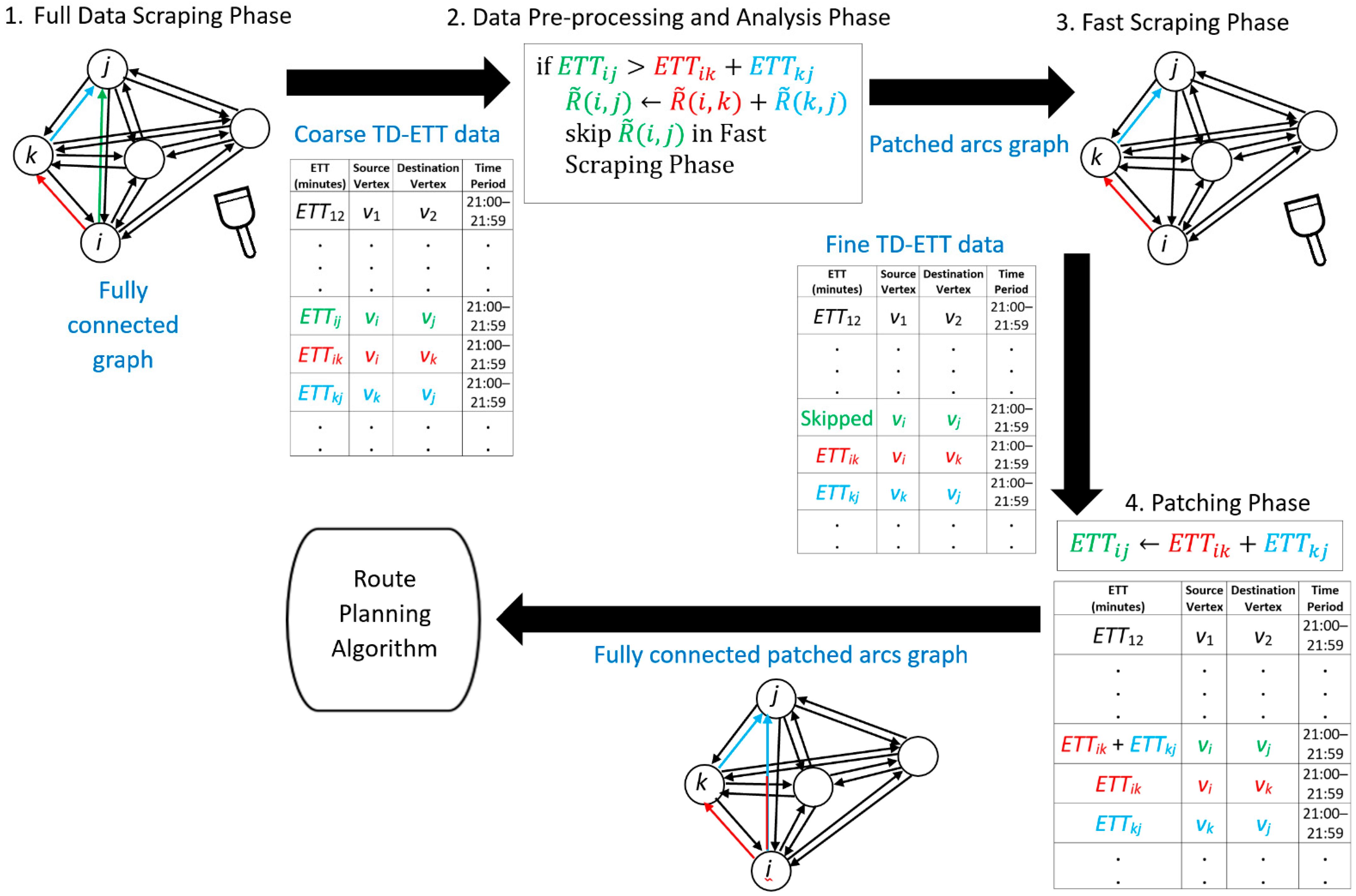
To remove the illogicality and redundancy of the directed graph, there are four phases of the framework that need to be carried out as shown in Figure 4. These phases are demonstrated and discussed with a case study in the following subsections.
3.1. Full Data Scraping Phase
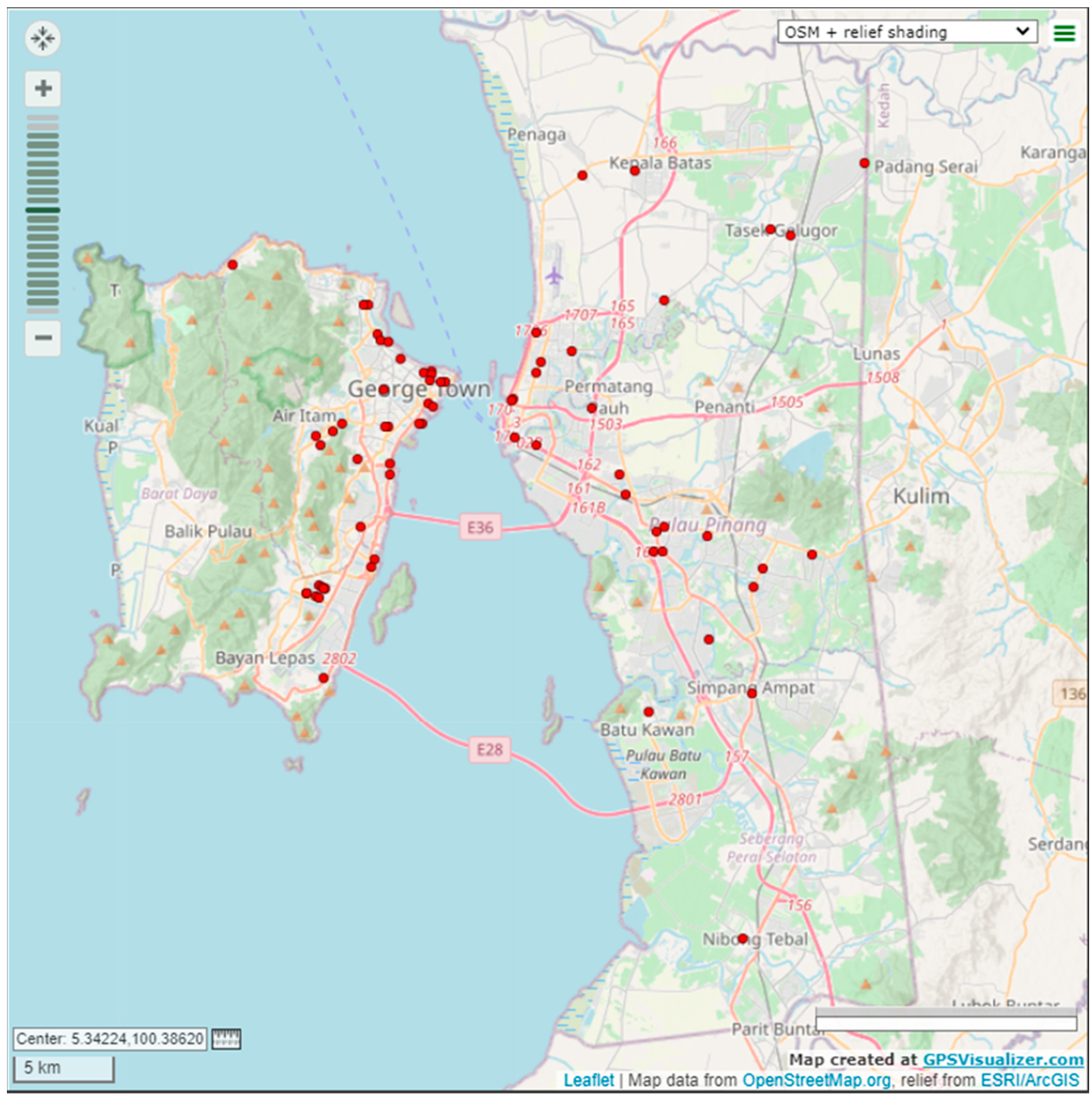
In this research, 68 vertices, each representing a logistic company outlet is considered, as shown at Figure 5.
It consists of 4556 arcs that construct a fully connected arcs graph. For the Full Data Scraping phase, all possible ETTs are collected continuously using the developed web scraper on web mapping websites. The objective of this phase is to collect complete initial data for analysis. All possible ETTs have to be scraped in order to provide every possible route to route planning algorithms for finding the optimal route; however, the time needed to complete an iteration of scraping is fairly long. Based on the results from 765 iterations of collected data, an average of 54.87 min is needed to complete an iteration of scraping a fully connected arc graph. Thus, fully scraping is not suitable for collecting data which requires a finer iteration in terms of time setting. This phase will last for weeks to collect as many iterations of data as possible, and these data will be fed into the next phase for preprocessing and analysis.
3.2. Data Pre-Processing and Analysis Phase
After scraping the full set of ETTs over different time periods for weeks, in the Data Pre-processing and Analysis Phase, the illogicality of the scraped ETT data in each time period will be detected and the alternative paths that consists of the combination of arcs with a shorter total ETT will be identified. The objective of this phase is two-fold. Firstly, the identified arcs with consistently illogical ETTs in each time period will be removed in the Fast Data Scraping phase so that the system can perform an iteration of scraping much faster in order to get a finer time-dependent data; secondly, arc-patching graphs can also be constructed in each time period so that the missing ETTs of the removed arcs can be patched with the ETTs of their respective alternative paths later.
During the examination on the scraped data, we found that the web mapping websites will not always provide the shortest arc between two vertices in a single iteration of scraped data because it does not fulfil Theorem 1. Thus, these illogical arcs need to be detected and their ETT values need to be rectified.
Algorithm 1 briefly outlines the pseudocode for detecting and patching illogical arcs.
In order to detect the illogicality, all scraped data are divided into different time periods, where each period has a duration of an hour. For the scraped data in a particular time period, they will be further split into a training set and a testing set.
In our approach, 85% of hourly data are categorized into the training set. Within this training set, if more than 70% of the data show that an arc consistently violates the inequality principle given in Theorem 1, then we will classify the scraped data of this arc as invalid, and thus the data needs to be removed and be patched later. Furthermore, the ETT of this arc will not be scraped in the future in order to shorten the scraping cycle; however, the unscraped ETT can still be patched with the alternative route that provides a shorter ETT route.
For the remaining 15% of the data, they are categorized as the testing set. The arcs that violated the inequality principle in Theorem 1 in the training set are patched with the corresponding alternative paths in the testing set, and they (the patched arcs), together with other unpatched arcs, form a full set of Partially-Patched ETT data. In order to verify the correctness and validity of the set of Partially-Patched ETT data, it needs to be benchmarked with the full set of original, unpatched data, which is called the Fully-Unpatched ETT data. The benchmarking is done through feeding both sets of data, respectively, to the TSP algorithm to find the optimal route by traversing around every vertex.
| Algorithm 1 Pseudocode for detecting and patching illogical arcs |
| 1. 2. 3. 4. do 5. do 6. do 7. 8. 9. 10. end for 11. end for 12. end for |
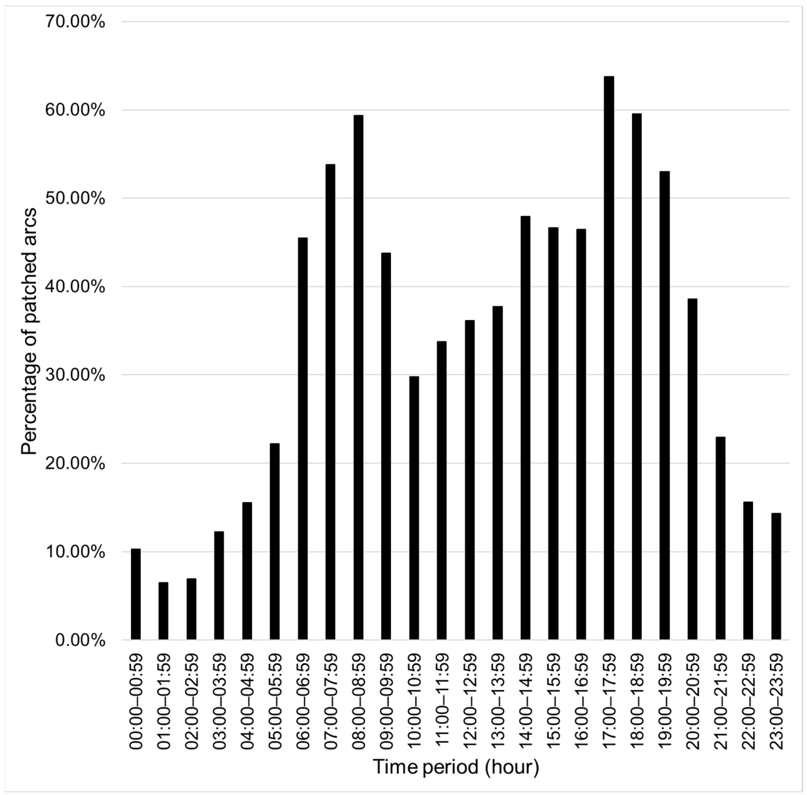
Based on the training data, an average of 34.26% (with a maximum of 63.78% and minimum of 6.50%) of arcs can be patched with shorter alternative routes in different periods from 00:00 to 23:59. The percentage of patched arcs of each hourly period is shown in Figure 6.
To verify the validity of the graph with patched arcs, the Simulated Annealing (SA) algorithm is used for benchmarking by solving the TSP with the derived Partially-Patched graph and the original Fully-Unpatched graph, respectively.
Initially, for each time period, T (say 12:00–12:59) on each day (say a specific Monday), the ETT data of the Partially-Patched graph are fed into the SA algorithm 10 times, and only the best resulted route (with shortest TSP travel time) among the iterations is stored.
This step will be done for the same time period, T (i.e., 12:00–12:59), over different days (say all weekdays with the scraped data), and then the average TSP travel time in this time period over all weekdays by using the relevant Partially-Patched graphs will be calculated, which is denoted by CP(T).
The similar process can be applied to the Fully-Unpatched graphs in the same time period, T (i.e., 12:00–12:59) over different days (i.e., all weekdays with the scraped data), and then the average TSP travel time by using the Fully-Unpatched graphs can also be calculated, which is denoted by Co(T).
Note that by comparing CP(T) against Co(T), we will be able to compare the results of the Partially-Patched graphs against that of the Fully-Unpatched graphs. Let the percentage of TSP travel time reduction be calculated as (4).
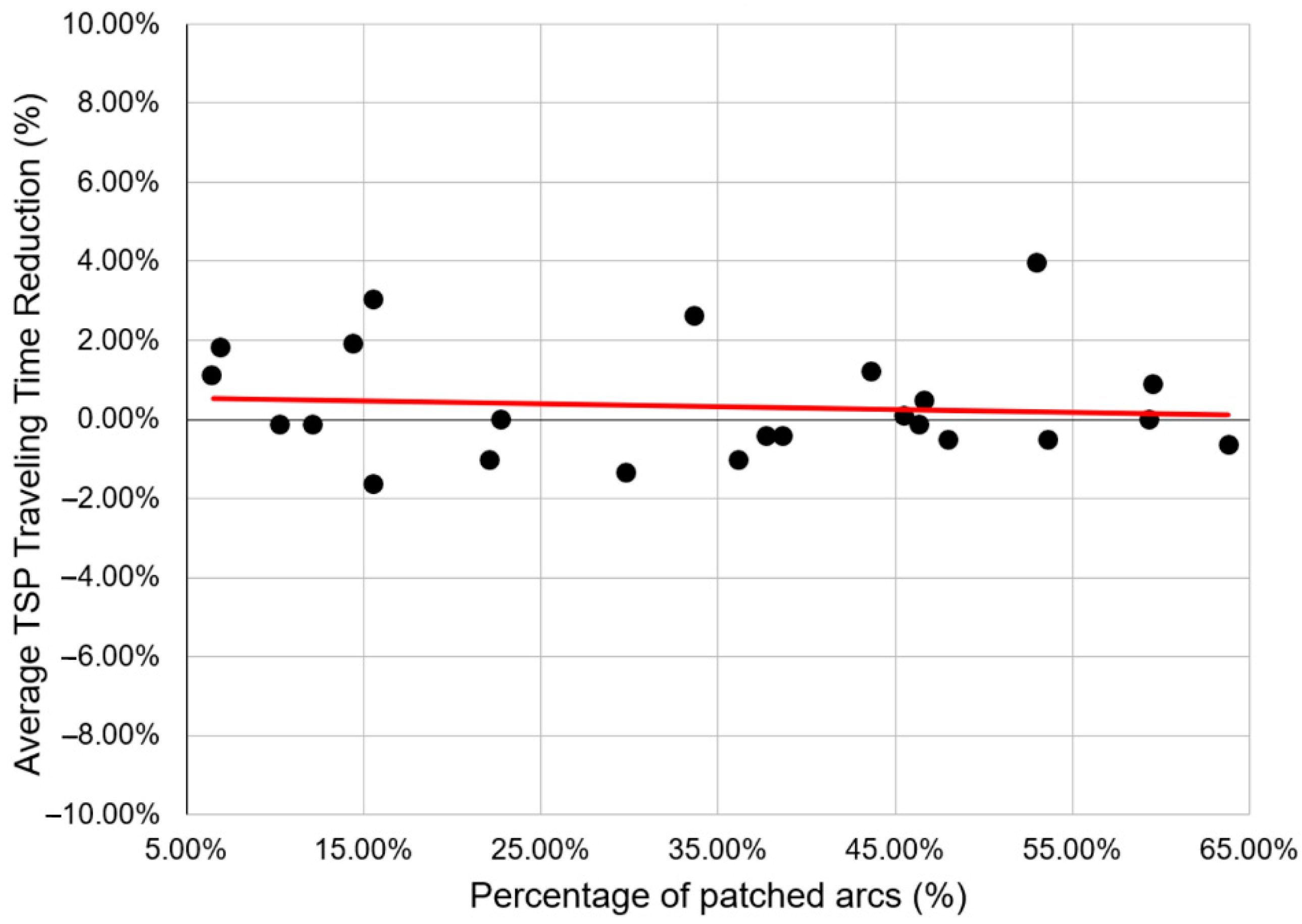
The percentage of TSP travel time reduction obtained from our experiment is plotted in Figure 7.
Figure 7 shows the percentage difference between the routing results generated with the Partially-Patched ETT data and the corresponding Fully-Unpatched ETT data. It can be noted that the difference is insignificant, that is, it is only in the range of −2% to 4%. The linear regression shows that majority of the patched graph data has positive difference. This also proves that the Partially-Patched graph is more likely to provide a shorter route than the original Fully-Unpatched graph, showing that the latter can actually be replaced by the former; therefore, arcs that violate the inequality principle of Theorem 1 can be skipped from web scraping in the future as there are alternative routes to patch them. This also improves the efficiency of web scraping as an average of 34.26% of arcs can be skipped from scraping.
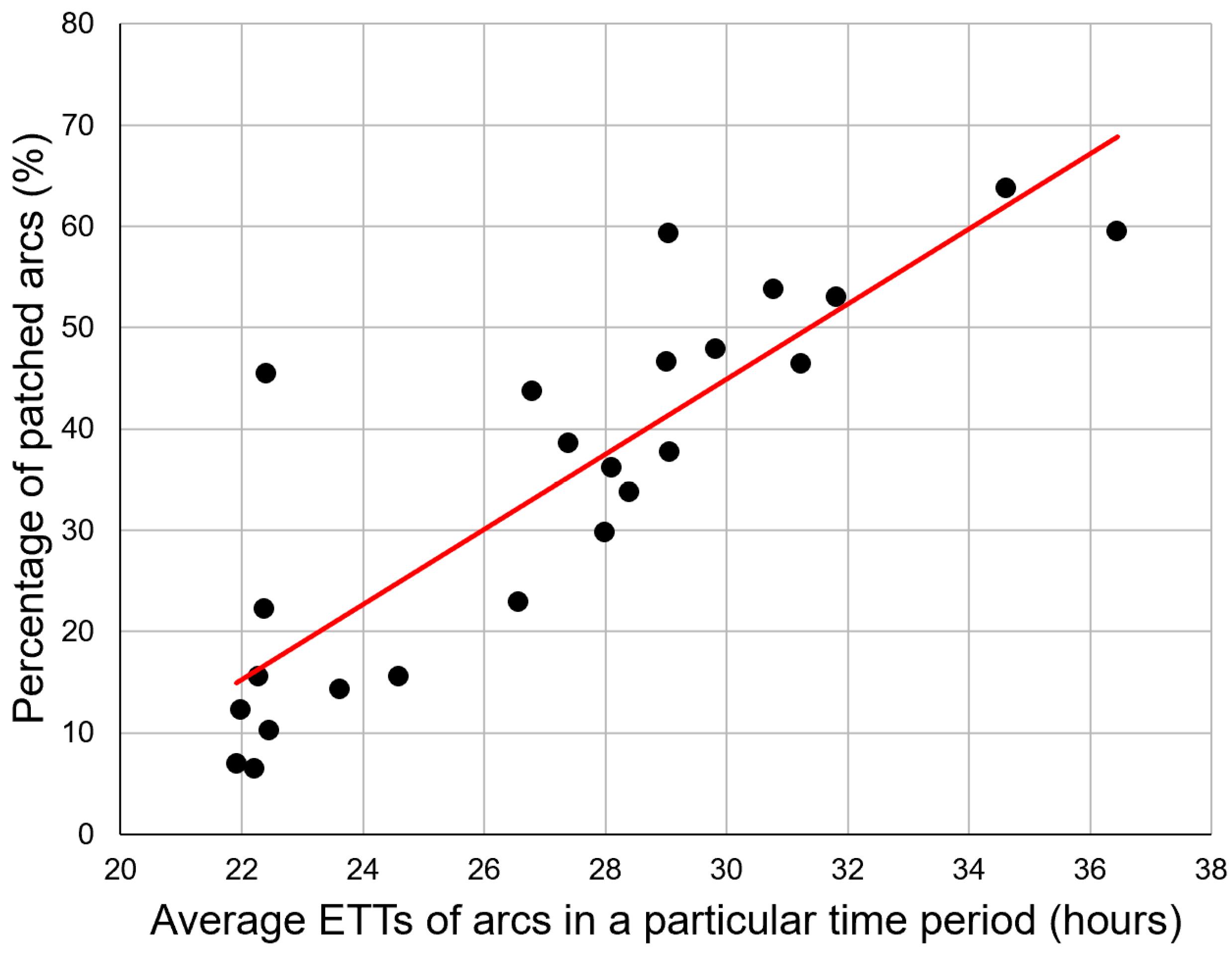
Moreover, the correlation score between percentage of patched arcs and average ETT of each subsequent hour is 0.8567, proving that the percentage of patched arcs is directly proportional to average TSP travel time. This is shown in Figure 8.
In actuality, the average ETT of each subsequent hour can be interpreted as the traffic condition. A higher average ETT indicates a heavier traffic condition. Moreover, the percentage of patched arcs indicates the correctness of the web mapping website to provide a shorter travel time arc. A higher percentage of patched arcs shows that a higher frequency of the ETT provided by the web mapping website is not optimal. As the average ETT increases, the percentage of patched arcs increases, proving the web mapping website is not likely to provide an optimal path when the traffic condition is heavier. This shows the importance of scraping traffic data efficiently and effectively by skipping arcs that will not be used frequently.
3.3. Fast Data Scraping Phase
After verifying the usability of the Partially Patched graph, in the Fast Data Scraping Phase, those arcs that can be patched (i.e., likely to have illogical ETT values) will be removed from being scraped, and thus the cycle of scraping can be shortened. The iteration time of the Fast Data Scraping Phase is much shorter than the Full Data Scraping Phase. Hence, more iterations of web scraping can be made, and a higher accuracy of traffic data can be obtained with finer details. This process will last for weeks to continuously scrape for ETT data.
3.4. Patching Phase
After the reduced scraping phase, the scraped data has to be patched during the patching phase, as an average 34.26% of arcs from the fully connected arcs graph are not scraped in the reduced scraping phase; therefore, these arcs have to be patched with the input of shortest ETT paths that consists of multiple arcs before solving TSP with route planning algorithms.
4. Experimentation and Results
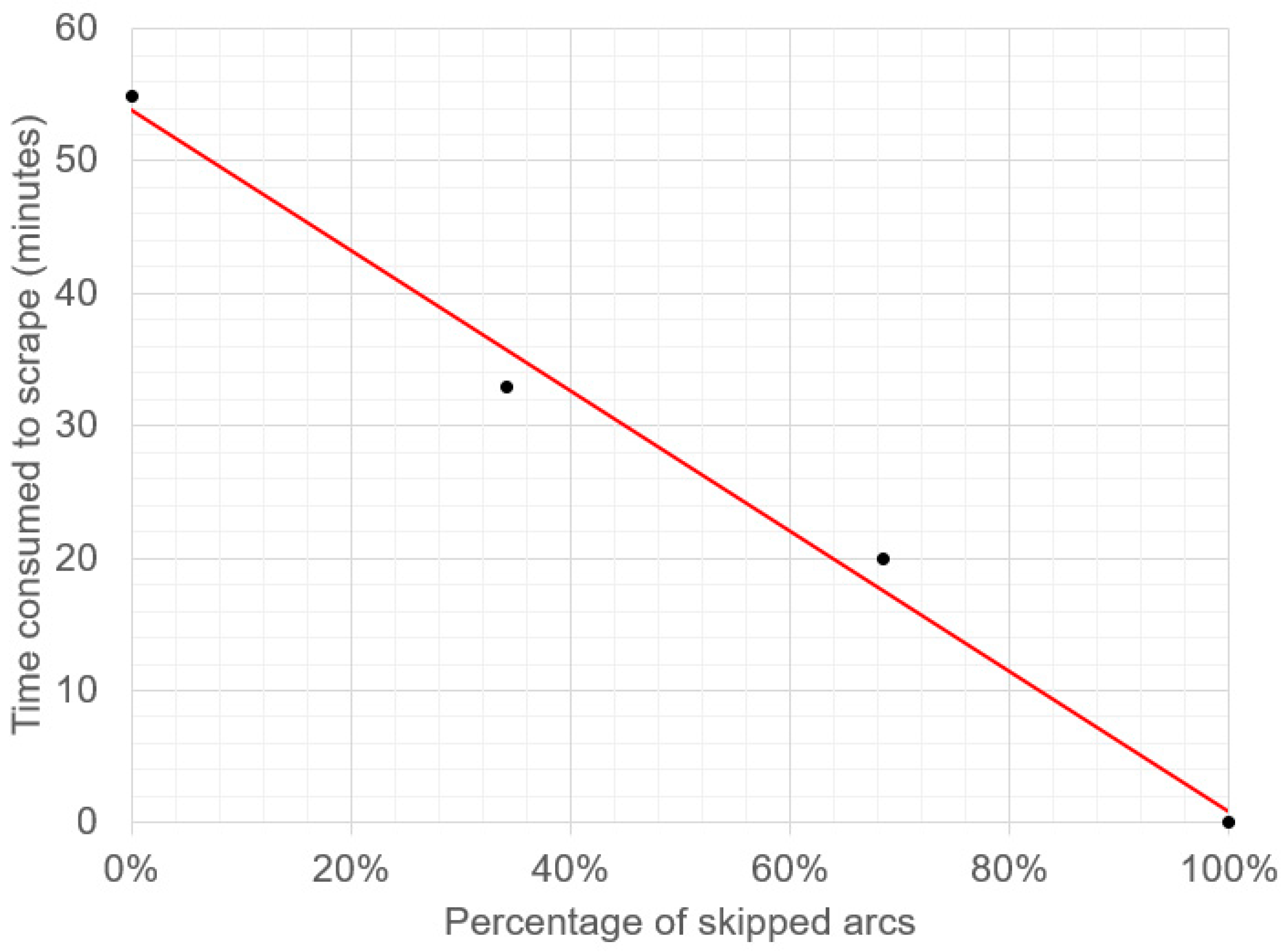
According to the scraped data from the Full Data Scraping Phase, an average of 54.87 min is spent to finish an iteration of web scraping. After skipping the 34.26% of illogical arcs in the Fast Data Scraping Phase, it only takes an average of 32.97 min to complete an iteration of web scraping, which is 40% faster than the Full Data Scraping Phase. Figure 9 shows the correlation between the percentage of skipped arcs and the time consumed to finish an iteration of web scraping. It shows the trade-off between the percentage of skipped arcs and the scraping duration, where one could choose to reduce the time consumption by skipping more arcs.
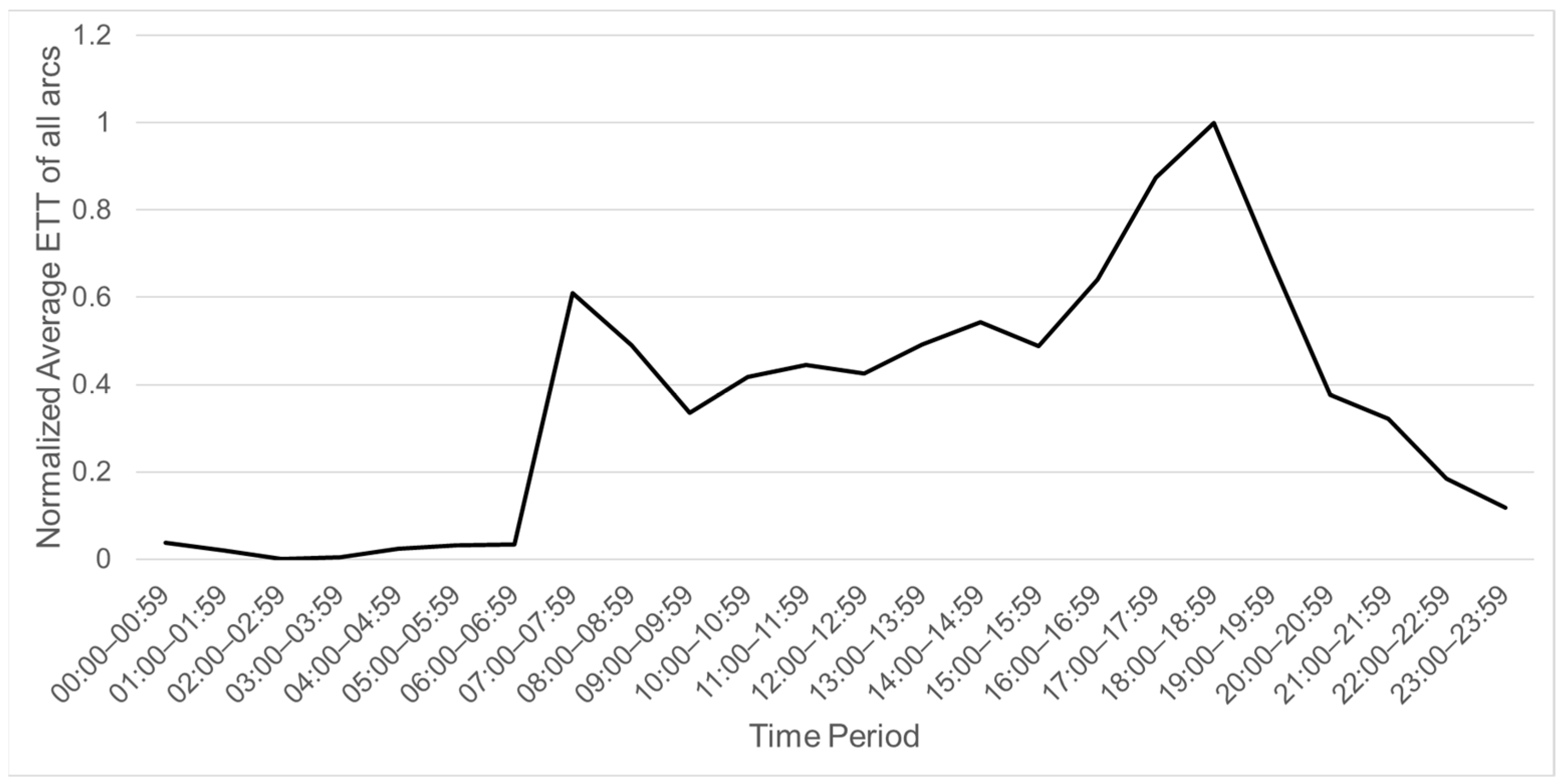
Based on scraped data, the traffic pattern can be classified according to different time ranges based on the normalized average ETT of all arcs, as shown in Figure 10.
According to Figure 10, the time from 07:00 to 08:59 and from 15:00 to 18:59 can be classified as the Peak period because the average traffic condition is much heavier compared with other times. Moreover, the time from 09:00 to 12:59 can be classified as the Normal period. Finally, other time ranges which are not within the Peak or Normal periods can be classified as the Traffic-free period.
As the arcs of traffic data in an iteration are not possible to be concurrently scraped, causing a time gap of an average 32.97 min between the first and the last arc, a ground truth is needed to justify the correctness of scraped data with the patched arcs graph. In this case, the ETT from the Google Distance Matrix API is used as our benchmark for comparison. This is because Google Distance Matrix API can collect an ETT of every arc within 1 min. The average TSP travel time during the Peak period and the Normal period are chosen for a comparison with the scraped data, as shown in Figure 11.
According to Figure 11, most of the average travel time to complete TSP from the Google matrix is higher than the scraped data, with an average of 6.17%. To ensure that the TSP route provided from scraped ETTs is applicable, the Google matrix’s ETTs are fitted into the route given by the scraped ETTs. Since the route is not optimal because of the fixed route from scraped ETTs, the average travel time of “Yellow” is 1.3% higher than “Blue”, with ranges between 1.5–7.0%. This shows the TSP route provided from scraped ETTs is applicable as there is only a 1.3% travel time difference compared to “Blue”, which is derived from the ETTs by using the Google Distance Matrix API. Without paying a huge monetary cost for the Google Distance Matrix API, even though the traffic data could not be instantaneously scraped using a web scraper, the TSP route provided from scraped ETTs does not bring much difference of the output of TSP travel time. This also verifies that our low-cost approach can be used to generate almost similar route planning results that can be generated by the data obtained from the paid Google Distance Matrix API.
One of the limitations of our proposed solution is that we only collected data within a city in Malaysia. In the future, data in other cities may need to be collected to test the model for further improvement. On the other hand, the interface or layout of the Google Map web page may change in the future; however, the data of interest will still be similar; therefore, we can use the same principle for data scraping but with a rearranged scraping position to reflect the changes in the web page layout. In addition, we only used one TSP algorithm to measure the cost of the route. In the future, we may fit the ETT data set into other VRP algorithms and simulation models [25].
Finally, the data scraped by our framework could be extended to include not only the ETT data, but also the sequence of roads in the recommended route. Such a sequence of roads actually forms a string. Thus, if we can compare the string data (i.e., recommended road sequences) of two arcs, then we can examine the similarity/dissimilarity between these two recommended routes using a string comparison framework, such as the one proposed by Cauteruccio et al. in [26]. Such information will be useful to improve our framework in the future.
5. Conclusions
In this paper, we have proposed a new cost-effective framework to effectively scrape, process, clean, and analyze TD-ETT data from free web-mapping services in order to gain knowledge of the traffic pattern in a city in different time periods. After scraping traffic data from free web-mapping websites, the collected data is then processed to detect arcs that violated the triangle inequality principle, from which we derived a theorem to pre-process, clean, and patch the TD-ETT values of these illogical arcs. In our experiment, we used the above framework to obtain the TD-ETT data over 68 locations in Penang, Malaysia, for six months. We then fed the data into a TSP algorithm for evaluation. We found that the performance of our low-cost approach is comparable with using the expensive paid data. By applying the framework proposed in this research in a real world scenario that consists of real-time traffic, a logistics company will be able to maintain the time-dependent estimated-travel-time data among locations of interest at a low cost, so that it can better plan the routes of its vehicles.
Author Contributions
Conceptualization, S.-Y.L., C.-S.W. and B.-Y.O.; methodology, H.-L.T. and S.-Y.L.; software, H.-L.T.; validation, S.-Y.L. and H.-L.T.; formal analysis, H.-L.T.; investigation, H.-L.T. and S.-Y.L.; resources, B.-Y.O.; data curation, H.-L.T.; writing—original draft preparation, H.-L.T.; writing—review and editing, S.-Y.L., C.-S.W. and B.-Y.O.; visualization, H.-L.T.; supervision, S.-Y.L., C.-S.W. and B.-Y.O.; project administration, C.-S.W.; funding acquisition, C.-S.W., S.-Y.L. and B.-Y.O. All authors have read and agreed to the published version of the manuscript.
Funding
This research was supported in part by the Malaysian Ministry of Higher Education under Fundamental Research Grant Scheme (FRGS) (FRGS/1/2018/ICT03/UTAR/03/1).
Institutional Review Board Statement
Not applicable.
Informed Consent Statement
Not applicable.
Data Availability Statement
Not applicable.
Acknowledgments
The authors would like to thank EasyParcel Sdn. Bhd. (1028666-H) and Exabytes Network Sdn. Bhd. (576092-T) for providing us data and resources to carry out our research.
Conflicts of Interest
The authors declare no conflict of interest.
References
- Watts, J. How Much Does GPS Fleet Tracking Cost? The Ultimate Guide. 2021. Available online: https://www.expertmarket.com/fleet-management/costs (accessed on 28 October 2021).
- Tee, H.L.; Liew, S.Y.; Wong, C.S.; Ooi, B.Y. Cost-effective scraping and processing of real-time traffic data for route planning. In Proceedings of the 2021 International Conference on Computer & Information Sciences (ICCOINS), Kuching, Malaysia, 13–15 July 2021; IEEE: Piscataway, NJ, USA, 2021; pp. 264–269. [Google Scholar]
- Ibrahim, A.A.; Lo, N.; Abdulaziz, R.O.; Ishaya, J. Capacitated vehicle routing problem. Int. J. Res. 2019, 7, 310–327. [Google Scholar]
- Qi, Y.; Cai, Y. Hybrid chaotic discrete bat algorithm with variable neighborhood search for vehicle routing problem in complex supply chain. Appl. Sci. 2021, 11, 10101. [Google Scholar] [CrossRef]
- Peng, P. Hybrid tabu search algorithm for fleet size and mixed vehicle routing problem with three-dimensional loading constraints. In Proceedings of the 11th International Symposium on Computational Intelligence and Design (ISCID), Hangzhou, China, 8–9 December 2018; pp. 293–297. [Google Scholar]
- Okhrin, I.; Richter, K. The real-time vehicle routing problem. In Proceedings of the International Conference of the German Operations Research Society (GOR), Saarbrücken, Germany, 5–7 September 2007; pp. 141–146. [Google Scholar]
- iFleet Plans & Pricing. Available online: https://ifleet.my/ifleet-gps-tracker-pricing (accessed on 16 September 2021).
- Kim, S.; Lewis, M.; White, C. Optimal vehicle routing with real-time traffic information. IEEE Trans. Intell. Transp. Syst. 2005, 6, 178–188. [Google Scholar] [CrossRef]
- Rathore, N.; Jain, P.K.; Parida, M. A routing model for emergency vehicles using the real time traffic data. In Proceedings of the 2018 IEEE International Conference on Service Operations and Logistics, and Informatics (SOLI), Singapore, 31 July–2 August 2018; IEEE: Piscataway, NJ, USA, 2018; pp. 175–179. [Google Scholar]
- Distance Matrix API Usage and Billing. Available online: https://developers.google.com/maps/documentation/distance-matrix/usage-and-billing?hl=en (accessed on 16 September 2021).
- Thomas, D.M.; Mathur, S. Data analysis by web scraping using Python. In Proceedings of the 3rd International Conference on Electronics, Communication and Aerospace Technology (ICECA), Coimbatore, India, 12–14 June 2019; IEEE: Piscataway, NJ, USA, 2019; pp. 450–454. [Google Scholar]
- Upadhyay, S.; Pant, V.; Bhasin, S.; Pattanshetti, M.K. Articulating the construction of a web scraper for massive data extraction. In Proceedings of the Second International Conference on Electrical, Computer and Communication Technologies (ICECCT), Coimbatore, India, 22–24 February 2017; IEEE: Piscataway, NJ, USA, 2017; pp. 1–4. [Google Scholar]
- What is Rate Limiting? | Rate Limiting and Bots. Available online: https://www.cloudflare.com/learning/bots/what-is-rate-limiting (accessed on 16 September 2021).
- Ghimiray, D. What is a Proxy Server and How Does It Work. Available online: https://www.avg.com/en/signal/proxy-server-definition (accessed on 16 September 2021).
- Residential Proxies Pricing. Available online: https://oxylabs.io/pricing/residential-proxy-pool (accessed on 16 September 2021).
- Narayanan, A.; Mitrovic, N.; Asif, M.T.; Dauwels, J.; Jaillet, P. Travel time estimation using speed predictions. In Proceedings of the 2015 IEEE 18th International Conference on Intelligent Transportation Systems, Gran Canaria, Spain, 15–18 September 2015; IEEE: Piscataway, NJ, USA, 2015; pp. 2256–2261. [Google Scholar]
- Yang, Q.; Gao, Z.; Kong, X.; Rahim, A.; Wang, J.; Xia, F. Taxi operation optimization based on big traffic data. In Proceedings of the IEEE 12th International Conference on Ubiquitous Intelligence and Computing and IEEE 12th International Conference on Autonomic and Trusted Computing and IEEE 15th International Conference on Scalable Computing and Communications and Its Associated Workshops (UIC-ATC-ScalCom), Beijing, China, 10–14 August 2015; IEEE: Piscataway, NJ, USA, 2015; pp. 127–134. [Google Scholar]
- Park, S.H.; Kim, S.M.; Ha, Y.G. Highway traffic accident prediction using VDS big data analysis. J. Supercomput. 2016, 72, 2815–2831. [Google Scholar] [CrossRef]
- Yuan, H.; Li, G. A survey of traffic prediction: From spatio-temporal data to intelligent transportation. Data Sci. Eng. 2021, 6, 63–85. [Google Scholar] [CrossRef]
- Noussan, M.; Carioni, G.; Sanvito, F.D.; Colombo, E. Urban mobility demand profiles: Time series for cars and bike-sharing use as a resource for transport and energy modeling. Data 2019, 4, 108. [Google Scholar] [CrossRef] [Green Version]
- Dantzig, G.; Ramser, J. The truck dispatching problem. Manag. Sci. 1959, 6, 80–91. [Google Scholar] [CrossRef]
- Ge, J.; Liu, X.; Liang, G. Research on vehicle routing problem with soft time windows based on hybrid tabu search and scatter search algorithm. Comput. Mater. Contin. 2020, 64, 1945–1958. [Google Scholar] [CrossRef]
- Novoa, C.; Storer, R. An approximate dynamic programming approach for the vehicle routing problem with stochastic demands. Eur. J. Oper. Res. 2009, 196, 509–515. [Google Scholar] [CrossRef]
- Baker, B.M.; Ayechew, M.A. A genetic algorithm for the vehicle routing problem. Comput. Oper. Res. 2003, 30, 787–800. [Google Scholar] [CrossRef]
- Kostrzewski, M. Implementation of distribution model of an international company with use of simulation method. Procedia Eng. 2017, 192, 445–450. [Google Scholar] [CrossRef]
- Cauteruccio, F.; Terracina, G.; Ursino, D. Generalizing identity-based string comparison metrics: Framework and techniques. Knowl. Based Syst. 2020, 187, 104820. [Google Scholar] [CrossRef]
Figure 1.
Example of four-dimensional data set.

Figure 2.
(a) An example showing there are three possible routes to travel from point i to point j on a geographical map; (b) the representation in a directed graph where the weight of the arc from vertex i to vertex j is the ETT of the best route from point i to point j on a geographical map.
Figure 2.
(a) An example showing there are three possible routes to travel from point i to point j on a geographical map; (b) the representation in a directed graph where the weight of the arc from vertex i to vertex j is the ETT of the best route from point i to point j on a geographical map.

Figure 3.
Travelling duration of an arc to time.

Figure 4.
Diagram illustrating the pipeline of proposed framework.

Figure 5.
Location of 68 outlets of a logistic company.

Figure 6.
Percentage of patched arcs in each time period [2].
Figure 6.
Percentage of patched arcs in each time period [2].

Figure 7.
Average TSP travel time reduction versus the percentage of patched arcs in the graph [2].
Figure 7.
Average TSP travel time reduction versus the percentage of patched arcs in the graph [2].

Figure 8.
Correlation between average ETTs of arcs in a particular time period and the percentage of patched arcs [2].
Figure 8.
Correlation between average ETTs of arcs in a particular time period and the percentage of patched arcs [2].

Figure 9.
Correlation between percentage of skipped arcs and the time consumed to finish an iteration of web scraping.
Figure 9.
Correlation between percentage of skipped arcs and the time consumed to finish an iteration of web scraping.

Figure 10.
Correlation between time period and the normalized average ETT of all arcs [2].
Figure 10.
Correlation between time period and the normalized average ETT of all arcs [2].

Figure 11.
Average travel time needed to complete TSP during Peak and Normal periods.


Table 1.
Comparison between different approaches for traffic data collection, adapted from [2].
Table 1.
Comparison between different approaches for traffic data collection, adapted from [2].
| Google Distance Matrix API [10] | Local GPS Service Provider [7] | Web Scraper | |
|---|---|---|---|
| Estimated cost per month (USD) | 26,242 (68 nodes) | 853.24 (50 vehicles) | Free |
| Flexibility | Low | Low | High |
| Implementation | Easy | Easy (Data incomplete) | Hard |
Table 2.
Notations/Abbreviations and Definitions.
| Notation/Abbreviation | Definition |
|---|---|
| A geographical region consists of vertex set V and arc set A | |
| V = {v1, v2, … vn} | The set of n points of interest in G |
| A = {(vi, vj)|vi, vj ∈ V, vi ≠ vj} | The set of arcs where each arc (vi, vj) refers to a route connecting point i to j in the real map |
| The route from point i to j with the shortest travel time | |
| The weight of arc (vi, vj), which represents the shortest travel time from i to j in the real map | |
| a = |A| | The number of arcs in the directed graph G |
| ETT | Estimated travel time |
| TD-ETT | Time-dependent estimated travel times |
Publisher’s Note: MDPI stays neutral with regard to jurisdictional claims in published maps and institutional affiliations. |
© 2022 by the authors. Licensee MDPI, Basel, Switzerland. This article is an open access article distributed under the terms and conditions of the Creative Commons Attribution (CC BY) license (https://creativecommons.org/licenses/by/4.0/).
Share and Cite
MDPI and ACS Style
Tee, H.-L.; Liew, S.-Y.; Wong, C.-S.; Ooi, B.-Y. An Estimated-Travel-Time Data Scraping and Analysis Framework for Time-Dependent Route Planning. Data 2022, 7, 54. https://0-doi-org.brum.beds.ac.uk/10.3390/data7050054
AMA Style
Tee H-L, Liew S-Y, Wong C-S, Ooi B-Y. An Estimated-Travel-Time Data Scraping and Analysis Framework for Time-Dependent Route Planning. Data. 2022; 7(5):54. https://0-doi-org.brum.beds.ac.uk/10.3390/data7050054
Chicago/Turabian StyleTee, Hong-Le, Soung-Yue Liew, Chee-Siang Wong, and Boon-Yaik Ooi. 2022. "An Estimated-Travel-Time Data Scraping and Analysis Framework for Time-Dependent Route Planning" Data 7, no. 5: 54. https://0-doi-org.brum.beds.ac.uk/10.3390/data7050054