1. Introduction
Computational Fluid Dynamics (CFD) is the simulation of transport phenomena, reacting systems, heat transfer, etc., using modelling, i.e., mathematical physical problem formulation and numerical solution, which include discretization methods, solvers, numerical parameters and mesh generation. The efficient and thorough development, implementation and evaluation of a suitable curriculum, which incorporates both the theoretical and practical aspects of CFD, for undergraduate students as an extension of their knowledge in the thermo-fluids area is warranted and necessary in modern engineering programmes. Numerical methods have an advantage over analytical methods of solution in that analytical methods tend to be restrictive by commonly requiring simple geometries, unrealistic assumptions and until lately assumed linearity, whereas real engineering problems usually have quite complex geometries and highly non-linear phenomena. However, despite the advantages of numerical methods, the latter may miss some finer aspects of fluid dynamics which, from the equations of analytical methods, may be more transparent, for example the question of uniqueness of weak solutions to Navier-Stokes equations in three dimensions. Analytical methods also often task a student to consider the treatment of any nonlinear terms found in partial differential equations, hence encouraging a student’s interest in this important topic.
Many areas of engineering education already use mathematical modelling as a teaching tool, for example, for diesel engine studies [
1], in fluid mechanics and heat transfer [
2,
3,
4] and in chemical reactions [
5]. It is important when introducing a complex topic such as CFD to have educational user-friendly interfaces, usually in the form of dialogue graphical user interfaces (GUIs), and some work has already been done on this [
6,
7], where the general aspects of the three main processes of CFD, i.e., building the problem using a pre-processor, solving the problem, and displaying the results using a post-processor were considered. However, although the education benefits associated with integrating computer-assisted learning and simulation technology into undergraduate engineering course are great [
8], and, computational fluid dynamics has revolutionized approaches to research and design, its incorporation into the teaching of undergraduate transport phenomena has still difficulties. One of these difficulties, and the one addressed in this paper, is to efficiently and thoroughly combine a sufficient understanding of the theoretical aspects of CFD with its practical use. Another is to engender a critical understanding of obtained results.
To help with an initial understanding of the process of solving Navier-Stokes and related transport equations the symbolic software,
Mathematica [
9] was employed to demonstrate the mathematical aspects of some of the basic steps involved, for example meshing, discretization, application of boundary conditions and the development of a simple solution algorithm. Two-dimensional incompressible flows were calculated for simplicity and the Navier-Stokes, at this stage of the course, were recast in an alternative form, i.e., in terms of streamfunction and vorticity. In many applications, the vorticity-streamfunction form of the Navier-Stokes equations provides a better insight into the physical mechanisms driving the flow than the “primitive variable” formulation which is in terms of the mean velocities
and pressure,
. The streamfunction and vorticity formulation is also useful for numerical work, since it avoids some problems resulting from discretization of the continuity equation.
The second part of this work outlines how to best introduce the practical aspects and emphasizes concerns which must be remembered when using CFD. Issues arise when introducing simulation into a curriculum, including learning vs. research objectives, usability vs. predetermined objectives and student demographics. A proper balance must be sought for between these competing objectives; for example, it is just as important that students are taught the systematic and practical ways of using a CFD package in a general sense, as well as achieving a specific result. There is evidence from previous studies that using simulation enhances the curriculum [
4]; there is increased learning efficiency and understanding [
10,
11]; there is effectiveness of hands-on learning methods [
12]; and, it is effective to use a combination of physical and simulation laboratories [
7].
Other concerns when introducing CFD to students are, for example, when to introduce during the programme, how much to introduce and how much mathematical and thermo-fluid backgrounds are necessary [
13]? When a student first commences studying CFD a lot of new knowledge and required skills descend on them from several different curriculum areas, which must be married together hence rendering a steep learning curve. If careful planning is not carried out, this curve may become overwhelming for many of the students. It is also important to ensure that the CFD GUIs are not treated as ‘black boxes’, without knowledge of what is going on inside the computer software. This is especially true as many commercial codes now provide the opportunity of attaching in-house coding to the main core of the software hence providing a gateway for enhanced research and code development [
14]. Without knowledge of CFD fundamentals and the core coding, code development would not be possible. It is important that students maintain a ‘feeling’ for physical phenomena, remember the necessary assumptions made for the mathematical modelling, and, very importantly, know of the need to verify and validate the calculated results [
15]. It has been observed that successful implementation of CFD often requires a re-focus of course objectives and skills taught, and a re-structuring of the course curriculum [
16]. An important practical consideration is to engender into the students a healthy skepticism concerning the calculated results and a willingness to be critical of their results until validated [
17].
In this paper the mathematical aspects of CFD are first introduced, with a particular emphasize on how to discretize equations. This is followed by a discussion of practical details such as closure of the Navier-Stokes equations using turbulence modelling, appropriate meshing within the computation domain, various boundary condition, properties of fluids, and the important methods for determining that a convergence solution has been reached. An overall description of the course is then given. The paper finishes with conclusions drawn and possible work needed for future development.
2. Numerical Elements of Computational Fluid Dynamics (CFD) Teaching
2.1. Introduction
In this part of the course, which lasted for four weeks, the purpose was to develop the basic steps involved in solving Navier-Stokes equations using a finite-volume approach for incompressible steady-state flow. The students can actually see the development of the mathematical description linked to a programming environment solution process, so often hidden in commercial code used for training CFD students. The students start with discretization of the governing equations, write their own coding to generate a mesh, apply boundary conditions, provide a suitable solution algorithm and to generate contour and x-y plots.
The students had already successfully completed courses on matrix algebra, vector calculus, ordinary and partial differential equations, with the latter solved using a variety of numerical methods, as well as preliminary courses on fluid mechanics and heat transfer. The students also have reasonable experience of using
Mathematica, which is a necessary prerequisite [
18]. Required reading for the course included LeVeque [
19] and Ferziger and Peric [
20].
In the following sections the theory taught to the students in preparation for them writing appropriate coding is summarized.
2.2. Navier-Stokes Equations
The governing equations for modelling fluid flow are the Navier-Stokes equations and the continuity equation. These laws of motion are valid for all phases including liquids, gases and solids, but there is a fundamental difference between fluids and solids in that fluids have no limit to their distortion. The analysis of fluid flow needs to take into account such distortions. The Navier-Stokes equations can be derived by the consideration of the dynamic equilibrium of a small fluid element and they state that surface and body forces are in equilibrium with inertial forces acting on the fluid element. On consideration of incompressible flow, where the density is constant, the Navier-Stokes equations for three-dimensional flow are as shown in Equations (1)–(4). Here body forces have not been included.
where
are the velocity components in the
directions,
is the fluid density,
is the pressure and
is the kinematic viscosity.
Most flows encountered in engineering problems are turbulent because it is mostly impossible to stop transition from laminar to turbulent flow, or, by intention, as turbulence may aid the engineering application. For turbulent flows however, the variation of the quantities to be calculated with time is often so rapid and with a high degree of randomness that this variation is of little engineering relevance. Hence the quantities are averaged and most often the Reynolds-averaged Navier-Stokes equations as shown in Equations (5)–(8) are used.
As can be observed, the instantaneous quantities are replaced by their corresponding time-averaged quantities. Extra terms appear due to the averaging process, e.g., and these behave like stress terms, often called Reynolds stresses, which need further equations if the system of equations is to be closed. There have, over this last 60–70 years, been many suggestions as to the best way for equation closure, none of which as yet are completely satisfactory.
2.3. Vorticity-Streamfunction Governing Equations
For this work, the Navier-Stokes equations are caste into the vorticity-streamfunction form, where the streamfunction is defined as
and where the integral has to be evaluated along a curve
from the arbitrary but fixed point
to point
,
is the velocity vector, and
is the unit normal on the curve from
to
. The streamfunction is regarded as a function of the spatial coordinates only. Streamlines are lines that are everywhere tangential to the velocity field, and hence
is constant along the streamlines. Invoking the integral incompressibility constraint for an infinitesimally small triangle shows that
is related to the two Cartesian velocity components
and
via
Flows that are specified by a streamfunction automatically satisfy the continuity equation since
For two-dimensional flows, the vorticity vector
only has one non-zero component (in the
direction; i.e.,
where
Using the definition of the velocities in terms of the streamfunction shows that
The Navier-Stokes equations for incompressible steady-state flow in vorticity-streamfunction form are
where
is the Reynolds number.
It should be mentioned that the above formulation is only valid in two-dimensions and some alternation is needed when three-dimensional flow is considered.
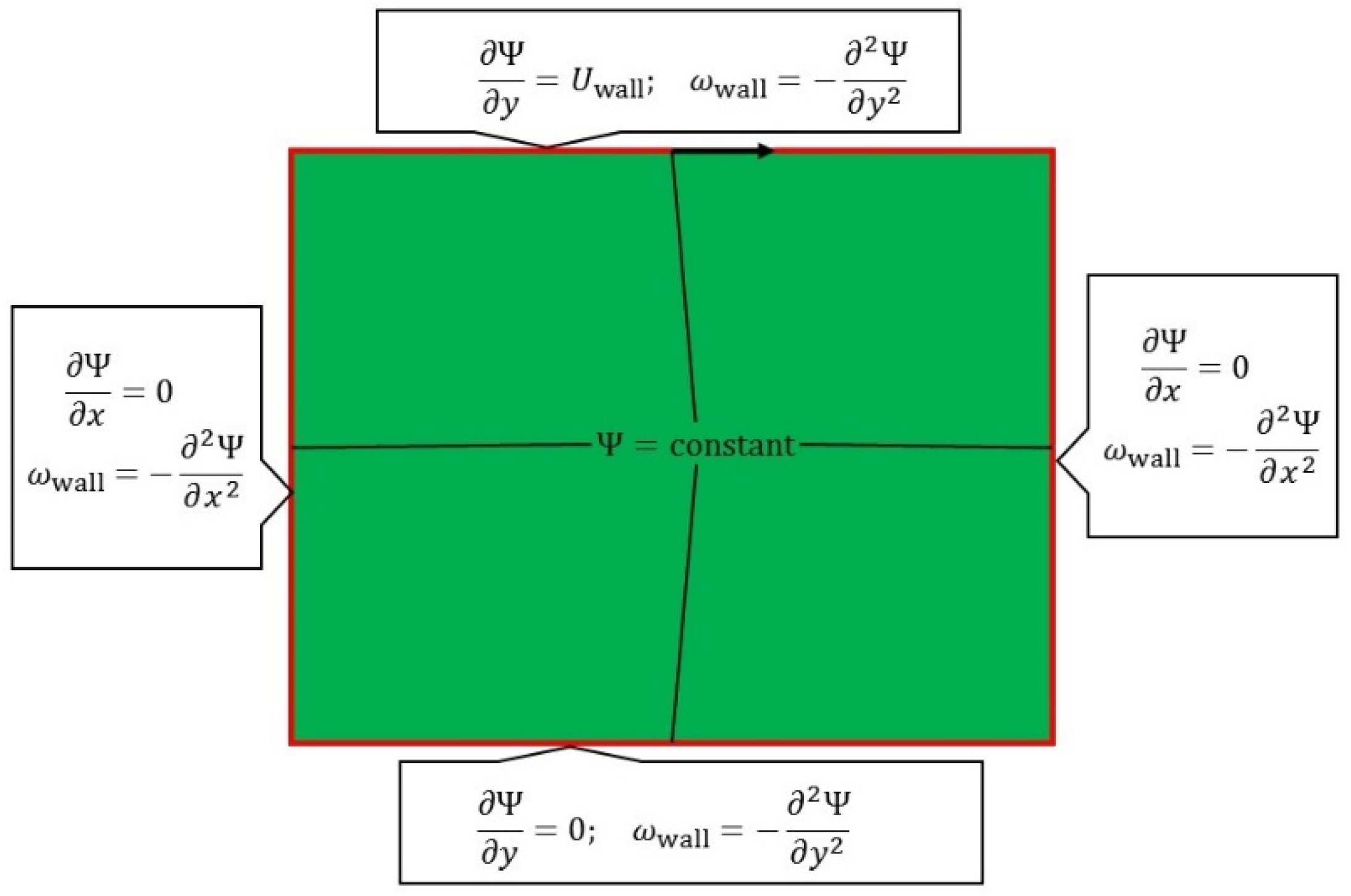
2.4. Boundary Conditions
The boundary conditions needed to solve Equations (14) and (15) for the classical computational fluid dynamics case, namely the lid-cavity flow [
21], are shown on
Figure 1.
A rectangular box, where the lid is allowed to move in the horizontal plane from left to right, is simulated with the moving lid driving the fluid within the box. In
Figure 1 the boundary conditions needed for solution are summarized in terms of vorticity and streamfunction. The streamfunction is constant at the walls, as its gradient is velocity, which is zero relative to a given wall (the no-slip condition). The vorticity boundary condition for each wall is also shown in each of the outer boxes and are derived from the streamfunction.
2.5. Discretization of Transport Equations
Before describing the discretization of the governing equations, it is important to note that for convenience Equations (14) and (15) together with the boundary conditions were non-dimensionalized using
where
and
are the height and width of the cavity, respectively, and
is a reference velocity. The resultant governing equations in vorticity-streamfunction format become
defined in the domain
.
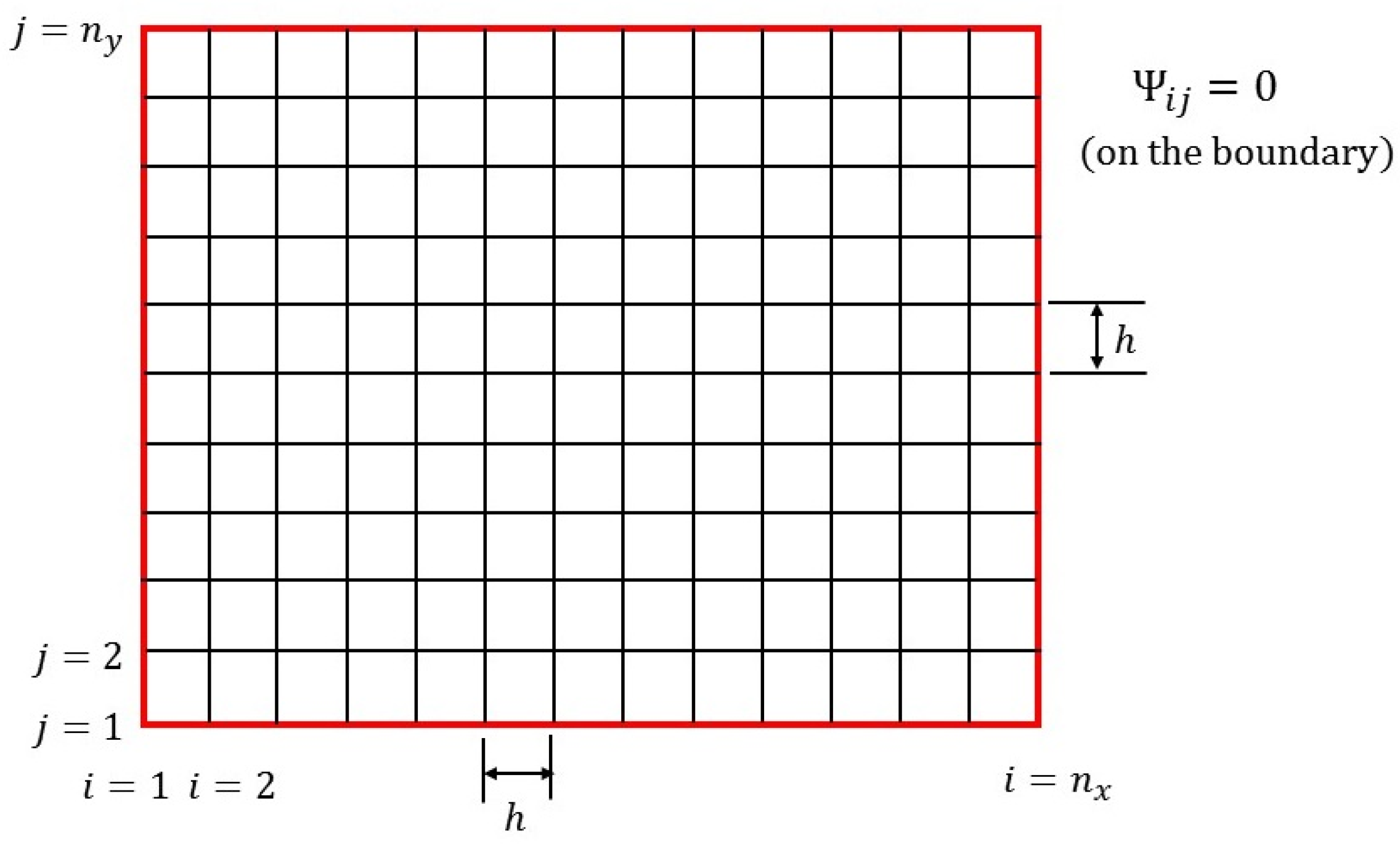
So as to include the boundary nodes of the cavity, central differencing is used to discretize Equations (16) and (17) with the number of nodes in the
and
directions set at
and
, respectively. The mesh is a regular Castesian grid with the nodes equally spaced at a distance
, as illustrated on
Figure 2.
To discretize Equations (16) and (17) the following central-difference approximations were introduced for spatial dimensions, obtained by adding or subtracting one Taylor series from another and invoking the intermediate value theorem. As can be seen from Equation (18), the order of accuracy for both the first and second derivatives is
Using the approximations from Equation (18), the discretized advection-diffusion equation (Equation (16)) at the
node is
The elliptic equation (Equation (17)) at the
node is
The equations are applied at the internal nodes of the Cartesian mesh; i.e., and .
2.6. Solution Algorithm
The iterative solution used here is based on Burggraf’s proposal [
23]. The solution method uses residual functions; i.e., if the values of
and
are exact on the nodes spanned by the residual functions
and
, then
where
The following fixed-point iterative procedure, based on the Gauss-Seidel scheme (see
Appendix A for a short general explanation), is then constructed
where
is a relaxation parameter lying in the range
, and
and
refer to the respective iterations. The use of this relaxation parameter is to improve the stability of a particular computation, particularly when solving steady-state problems.
The boundary conditions now need to be determined. For the streamfunction
For vorticity, the following needs to be considered for, say, the left wall of the cavity with one node outside the computational domain.
The value of
can be accounted for by using the no-slip boundary condition on the cavity wall, i.e.,
Using central differencing, this condition can be written as
where again the order of accuracy is
.
This finding, together with
gives
Similarly, for the other walls of the cavity the boundary conditions for vorticity can be deduced from
to give
It should be noted that the final boundary condition shown in Equation (30) is for the moving lid, and the extra term is due to the tangential velocity being non-zero.
3. Practical Elements of CFD Teaching
3.1. Introduction
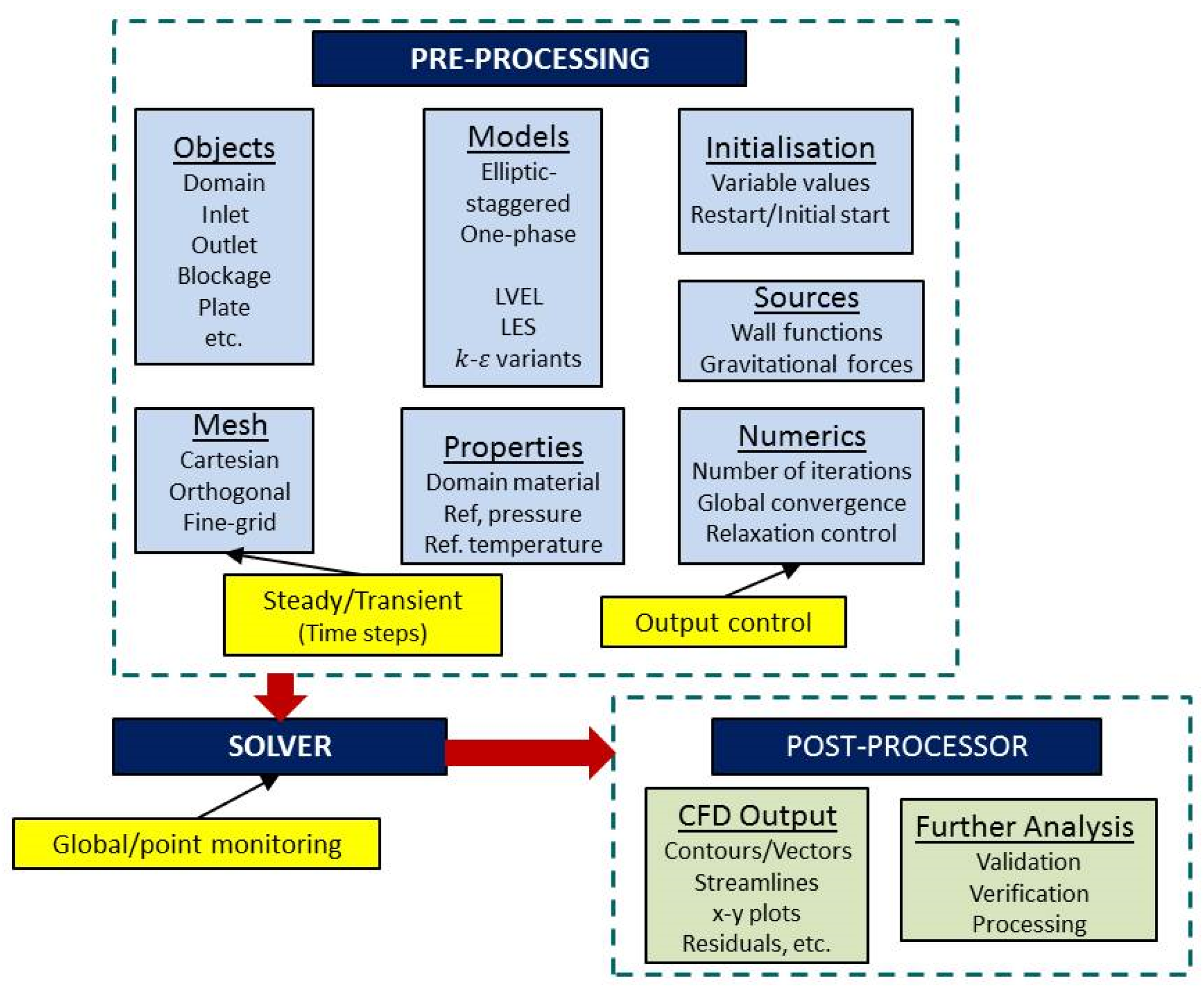
For Computational Fluid Dynamics laboratories, each student had a desktop computer on which was loaded software which provides the interface as a ‘three-dimensional’ fully interactive environment. The interface uses the concept of ‘virtual reality’ and allows a student to simulate a flow, including geometry, properties, boundary conditions, closure of equations, numerics, etc, from beginning to end without having to resort to specialized codes, or code writing. The code used can be used for professional engineering consultancy, so giving students useful skills and experience which contribute to their preparation for the workplace. The virtual reality (VR) environment is designed as a general purpose CFD interface, which can handle such problems as fluid flow, heat transfer, reacting flows, or a combination of all, and consists of the VR-Editor (pre-processor), the VR-Viewer (post-processor) and the solver module which performs the actual calculations. The VR-Editor allows a student to set the overall computational domain size, define the position, size and properties of object introduced into the domain, specify the material properties which occupy the domain, specify inlet and outlet boundary conditions, specify initial conditions, select turbulence models (if necessary), specify the fineness and type of computational mesh, and set the numerics by choosing a suitable solution algorithm and which influence the speed of calculation to obtain a convergence solution. Once the student is satisfied with problem set-up in the pre-processor, calculations are made using the solver module and the progress of the calculations is clearly monitored on-screen until convergence is reached. The results of the flow simulation are then displayed on the VR-Viewer graphically or they can be analysed from the raw numerical data. The post-processing graphical capabilities are vector plots, contour plots, iso-surfaces, streamlines and x-y plots.
3.2. Interface Design Features
The Computational Fluid Dynamics laboratory is designed in a user-friendly way, the computational features are easy to access and implement. It is important to keep parameter settings at the top level, and not to use multi-levels, as much as possible, as the setting of vital parameters necessary to the success of a particular simulation may well get hidden or even forgotten about, thus frustrating the student with strange results. Also it is important to show students that CFD methodology needs to be systematic and rigorous, as the laboratory must reflect what is found in engineering practice.
The CFD interface was designed, as shown on
Figure 3, so that the features systematically inform, it is vocationally sound and is easy to use.
Each simulation process reflected the situation in engineering practice with students systematically setting up the problem, solving and finally analysing the results. The students interact with the software using mouse and keyboard input with no requirement for the distraction of computer language coding so enabling them to concentrate on the CFD methodology and procedures and how close to reality their results are. An important feature of the CFD interface is that it is stand-alone, by which is meant that the problem-building, solving and post-processing are all combined in the same virtual reality environment. Also important is that all the data representing the results can be moved to the familiar Microsoft Office environment for further processing and reporting. The CFD software package operates on the Windows OS platform using PCs with relatively low computer power, and so the solvers have to be reasonably fast because the students have limited guided time in the laboratories, and also to keep their level of interest heightened, calculated results should come back reasonably quickly. In addition to producing contour plots, vector plots, etc., the post-processor could also produce animation for transient flows.
3.3. Example to illustrate use of the Interface
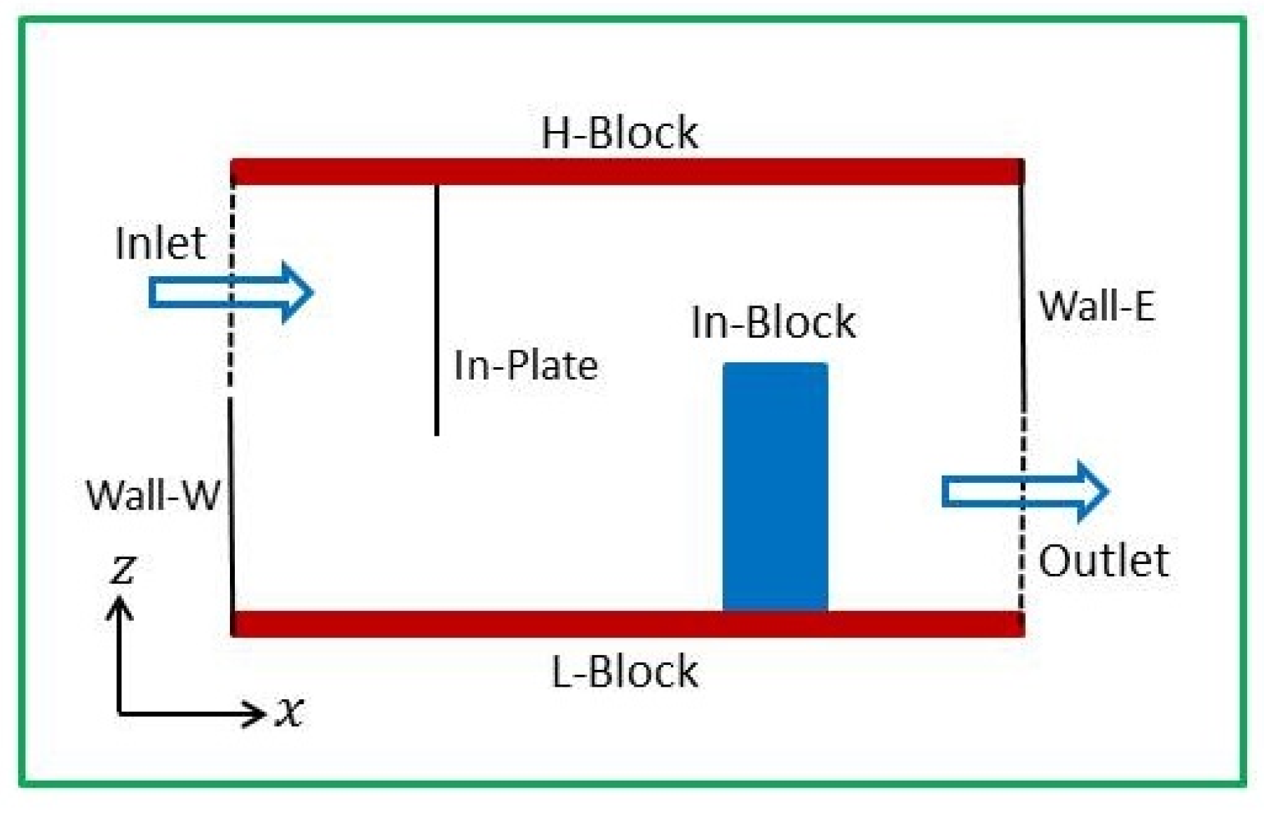
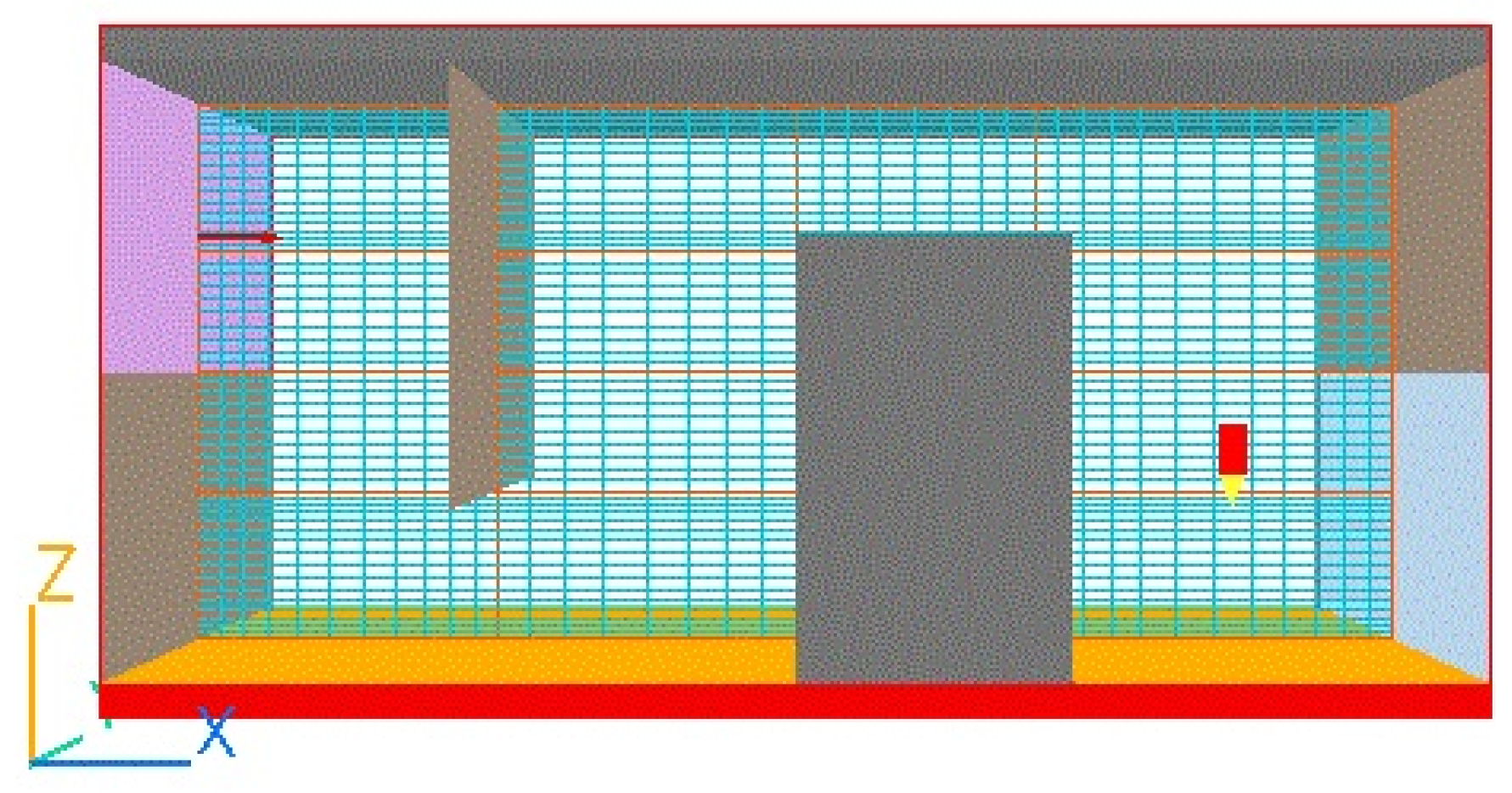
An example of flow through a labyrinth with heat exchange is given to illustrate the simplicity of the interface. The geometry is 2D with dimensions and the content of the computation domain is summarized on
Figure 4.
Initially the pre-processing virtual reality GUI is opened and the case title immediately entered. With reference to
Figure 3, under ‘Objects’ the x-domain size is changed to 2.0 m and under ‘Mesh’ a Cartesian grid is chosen. Under ‘Properties’, the user now checks that the default properties for this case are chosen, i.e., ‘Air at 20 °C, 1 atm’, the ambient air is set at 20 °C, and the ambient pressure is set at 0 Pa relative to 1 atm.
Under ‘Models’ the ‘solution for velocities and pressure’ is left ON, the ‘energy equation’ is clicked and ‘Temperature’ is selected. The turbulence model selection is left as the KE variant ‘KECHEN’.
Under ‘Objects’ each of the objects within the domain are selected, sized and positioned and where necessary given the relevant attributes. The objects introduced in order are, the H-BLOCK whose attribute is ‘ALUMINIUM at 27 °C. the L-BLOCK whose attribute is ‘ALUMINIUM and which is a HEAT SOURCE of 100 W’, the WALL-E which is a plate, the WALL-W which is a plate, the IN-PLATE, the IN-BLOCK whose attribute is ‘COPPER’, the INLET whose attribute is velocity in the x-direction at 0.5 m/s and whose temperature is ‘AMBIENT’, the OUTLET which has ‘PRESSURE’ as its attribute.
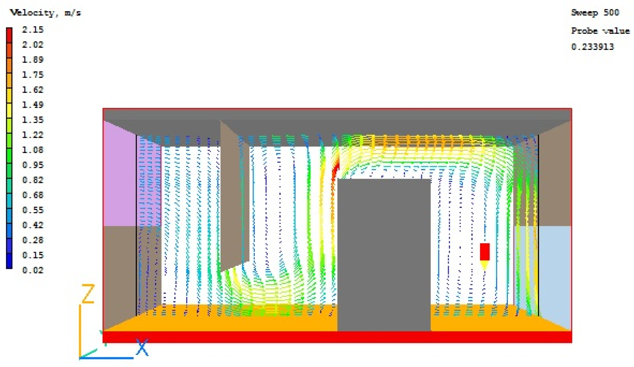
Once the basic geometry is in place, a computational grid is automatically suggested and can be inspected by the ‘MESH’ toggle, which for the present case, generates a picture as shown on
Figure 5. The grid can be customized to the user’s wishes simply by clicking on ‘Grid Mesh Setting’ and adjusting the default numbers.
In this example, ‘Initialisation’ and ‘Sources’ are taken as the defaults, and so only ‘Numerics’ is left to inspect and adjust. Here the number of iterations is set and the convergence tolerances are left at default. Importantly the probe used as one measure of convergence is appropriately positioned, i.e., not too close to the inlet or not placed in an anticipated region of recirculation.
The solver is now activated to perform the simulation. The progress of the calculations is displayed in relation to convergence, number of sweeps of the computation domain completed and the estimated time left to complete the simulation.
Once the solver has closed, the GUI post-processor can now be opened to view the results. Toggles are available to view ‘Vectors’, ‘Contours’, ‘Streamlines’, Iso-surfaces’, and further toggles are available to select which calculated variable is of interest. The results can be viewed on any plane or at any angle by the use of direction and rotation buttons respectively. A typical result is shown on
Figure 6 for a vector plot.
The students are shown how to save their work, and how to transfer results suitable for reports and further analysis.
3.4. Implementation of the CFD Laboratories
The Computational Fluid Dynamics laboratories were introduced using a combination of short-lectures on back-ground theory, demonstrations, student group work and discussion, and assisted hands-on computer usage over an intensive four week period. Gradually, as time passed, the students became more confident and were able to navigate their way around the software efficiently and with assurance. The format of the demonstrations was that the instructor built simple simulations while students, watching a large overhead screen, did the same operations on their own computer. Group work was also used where perhaps a group of four students were given an exercise and asked to build a simulation. This proved a very effective and efficient way of learning. Gradually the method of delivering instruction changed over the four weeks, from demonstrations, to the use of detailed instruction sheets fully supported by faculty and teaching assistant intervention, to the distribution of descriptions of problems without instructions or hints and only the occasional help from support staff. There was never any restriction in seeking help from other students (again something which happens in engineering practice).
The main learning outcomes during this part of the course were to become familiar with the equations that govern steady and transient fluid flow and heat transport (conservation of mass, momentum, heat, species and energy) and be able to apply these equations to a range of practical problems in the areas of fluid flow, heat transfer and species transport. Seminars were given to inform students of what was expected during the CFD laboratory. It was stressed that the students should not compartmentalize theory, experiments and computational fluid dynamics but rather view them as mutually complimentary. The main bulk of these seminars was the introduction of the students to standard CFD methodology and procedures and the splitting of the CFD process into three distinct procedures, i.e., pre-processing, solving and post-processing.
During this four week section of the course, theoretical fundamental topics covered included:
Getting started;
CFD notation;
CFD equations-continuity, momentum, energy, concentration of species;
Finite differencing;
The finite-volume method;
Boundary conditions;
Accounting for the pressure term;
Closure of averaged equations;
Time-stepping techniques; and,
Properties of numerical methods.
This section of the course included discussions on CFD good practices and importantly the students were taught to be critical of their results and how to examine if what they got as results is what they might have expected. During the hands-on sessions, the following areas listed in
Table 1 were emphasized.
4. Discussion
4.1. Overall Course Description
The main learning outcomes of this course are to understand how to apply the equations of transport governing conservation of mass, momentum and energy in an open and transparent way, and to be able to apply them correctly to a range of practical projects, including
predicting drag forces on bluff, streamline bodies and flat plates;
analyzing the flow in pipe systems;
analyzing performance of radial flow pumps and turbines; and,
matching pumps and turbines for particular applications.
The overall course last twelve weeks and was conducted during the fifth semester for students of mechanical and aerospace engineering, with 38 students taking the course. The first four weeks were used to teach the numerical aspects of computational fluid dynamics using close integration between theoretical lectures and hand-on computer laboratories, using as already described, mainly Mathematica, although some exercises using the versatile Python computer language were also introduced. The course during the second four weeks still had theoretical aspects within it, mainly in the form of turbulence modelling, but tended to concentrate on giving the students skills so as to solve real, though simple practical problems. The last four weeks of the course involved the students carrying out the series of projects outlined above, either individually or in small groups, which at first were supplemented with guidance and hints from the instructors on how to solve, but gradually this moved to problem description only, and it was left entirely to the student or students on how to enact a solution. In addition to set class time during these four weeks, the laboratory was open to students at any time, and discussion between the students was actively encouraged.
Assessment of students was by a series of bi-weekly quizzes and by assignment. No final examination was used.
4.2. Use of Mathematica
Based on the governing equations and boundary conditions established in
Section 2, the students had to individually write coding using the symbolic software,
Mathematica [
9], to solve the problem of a lid-cavity flow [
21]. The students had to write coding which set-up the required geometry, the mesh parameters and initial and boundary conditions. Next came coding for Eqns. [
14] and [
15], i.e., for
and
followed by coding for the iterative algorithm.
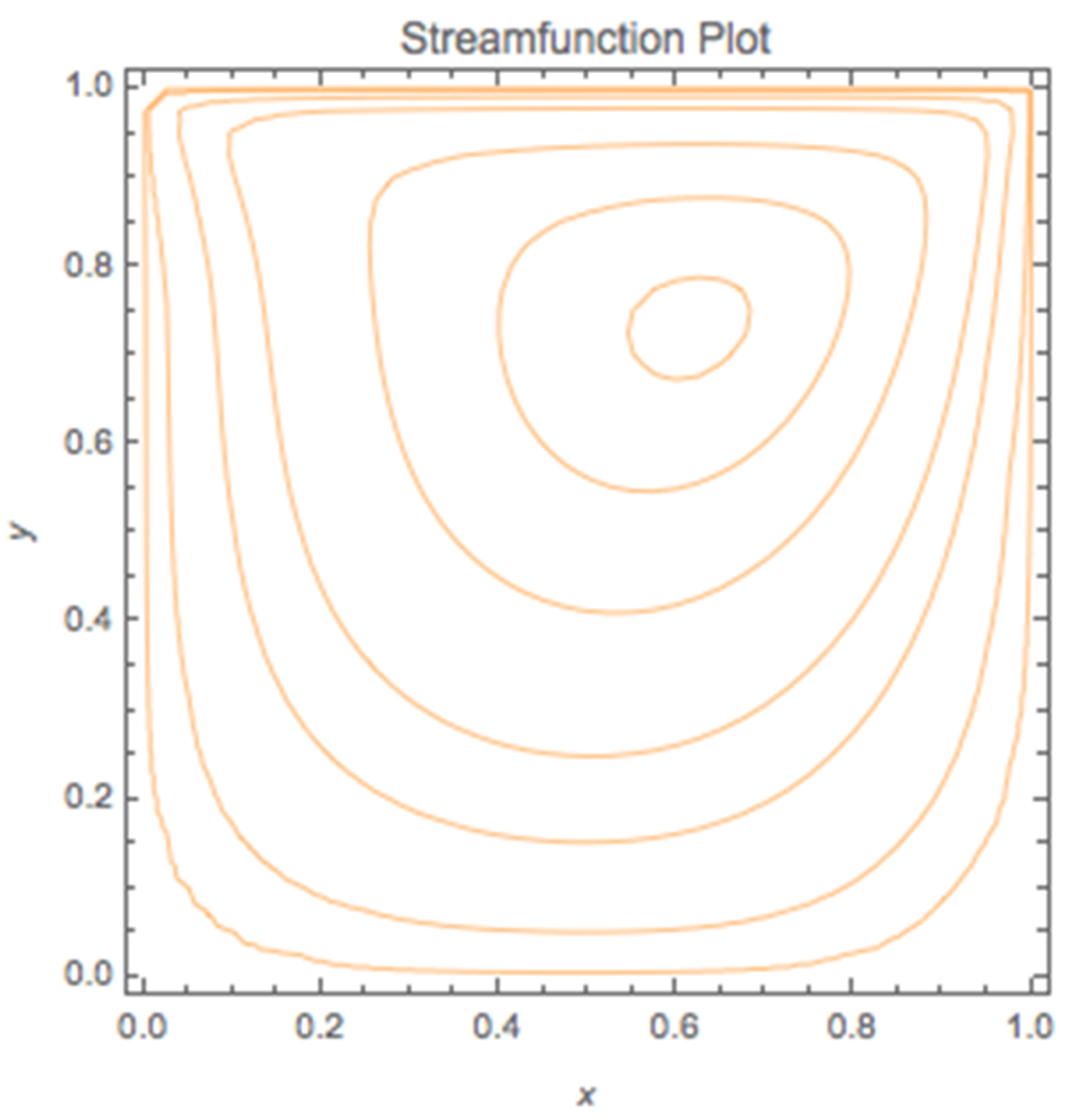
The mesh size for this problem and grid spacing had to be defined, and initially and were set to zero for all nodes, except the top wall, where the vorticity is non-zero. The Reynolds number was set to 100, the relaxation parameter, to 1 and the aspect ratio to 1. The students also had to set an appropriate residual value and carefully nest the loops used to execute the iterative algorithm. At every iteration step , if the maximum value of the absolute value of is less than , then the calculations are halted. The iterative loops were wrapped with the Mathematica function Timing to give an estimate of the time taken to do the calculations.
Following completion of the calculations, students had to then write coding to display contour and vector plots of their results. An example of a contour plot obtained for the streamfunction is given on
Figure 7.
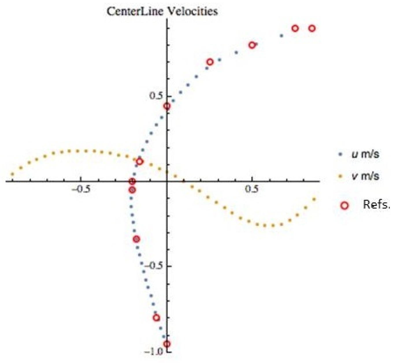
Extraction of the centerline velocities was also instructive for the students in that first, students were given more experience of viewing velocity profiles, and second there are ample calculations and measurements of the lid-cavity flow for comparison with their results [
25,
26,
27]. The centerline velocities
(in the
direction) and
(in the
direction) were derived from the streamfunction values using the equations
The velocity distributions for
and
in
Figure 8 are drawn along the vertical and horizontal centerlines, respectively.
Importantly, the students were made aware that the profiles they calculated must be compared, preferably with experimental measurements, to test the validity of their calculations. As can be seen from
Figure 8, the calculations for the horizontal centerline velocities compare very favourably with those reported by [
25,
27] for
. Finally, the students were asked to produce coding which displayed the formation of the streamfunction contour plot with time.
4.3. Computational Fluid Dynamics methodology
In the second third of the course, the students moved on to the skills involved when using CFD in a professional consultancy capacity, while still learning necessary underpinning theory. The idea of fluid mechanics theory, experimental work and the current CFD skills and knowledge being acquired as complementary was reinforced. CFD now has well established methodology coupled with good practice and procedures, and it was emphasized that following these carefully would produce results much more efficiently and with a better degree of confidence. The students were taught how to use CFD judicially and appropriately, and to check their work against experimentation where possible. The idea of breaking the CFD process into three distinct tasks was again reinforced, i.e., using the pre-processor to build the problem, using the solver to obtain a converged solution and the use of the post-processor to obtain informative results. The numerical process of discretization was especially reinforced, as was how to activate the acquired conservation equations, geometrical aspects, fluid and solid properties, activation of sources, especially the gravity or body force, numerical details, which included initialization, the iterative process and how to use under-relaxation when necessary. Setting of the boundary conditions correctly was taught as was how to close the conservation equations by using an appropriate turbulence model [
28,
29]. When results were achieved it was extremely important that students could interpret what they had got in light of, say, geometric considerations, and also to be open-minded and critical.
During the demonstrations on how to use the GUI interface it was felt important that students could have ‘hand-on’ experience rather than just watching. Several simple three-dimensional flows were used as exemplars to give an over-arching view of the CFD process and the virtual reality environment which facilitates the VR-Editor (pre-processor), the VR-Viewer (post-processor) and the solver module which performs the calculations was introduced.
It was demonstrated how the VR-Editor is used to set the size of the computational domain, define the position, size and properties of objects introduced into the domain, specify the materials which occupy the domain, specify inlet(s) and outlet(s) and other boundary conditions, specify chosen initial conditions, select a turbulence model (when appropriate), specify the fineness of the computational grid and set parameters which define convergence and also influence the speed of convergence of the solution procedure. Viewing movement controls were also discussed which zoom, rotate, and allow for vertical and horizontal translations. It was emphasized how to systematically create a new environment for a particular simulation and finally set an appropriate number for the maximum number of iterations, set the position of the monitor for convergence. Finally, the students were encouraged to review the computational domain, especially in regard to position and attributes of the objects and the refinement of the grid close to solid surfaces, which at this stage of the demonstration would not be appropriate.
The convergence to a solution was monitored in two ways. First a point in the computation domain was chosen and values of the variables updated after each successive sweep. Once the values became constant it was assumed a converged solution was obtained. This was backed up by calculating the ‘global errors’ or changes between successive sweeps through the computation domain for each variable and when these errors were deemed sufficiently small, convergence was declared.
Once a converged solution was obtained, the simulation results were viewed by way of the post-processor facilities which displayed vector plots, contour plots, iso-surfaces, streamlines and x-y plots. The students were encouraged to find the optimum way of presenting their results and were also instructed on how to print the results. Very importantly, they were taught to always save and catalogue all input and output files.
4.4. Individual and Group Projects
For the last four weeks of the course the students were given a series of assignments which got progressively more difficult. The projects were wide ranging and covered important topics, such as the use of orthogonal grids, fine-grid embedding, cut-cell techniques, further exploration of turbulence models and how appropriate they are, the volume of fluid technique and two-phase flows (solid/gas and liquid/gas). Several projects covered how to import complicated geometries, built using a computer-aided drawing (CAD) package. In addition to problems involving purely fluid flow, projects were included which expanded to flow combined with heat transfer, the modelling of species transport and gaseous combustion. Use was made of the non-premixed combustion model where a natural gas combustion problem was set and solved using the non-premixed combustion model for the reaction chemistry. A project was also included which modelled an evaporating liquid spray where several discrete-phase models, including wall surface reactions were included.
During this part of the course the teaching model used emphasized active and collaborative learning in addition to students and instructors discovering and constructing knowledge and techniques together. Outside of assignments set for grading, the students were encouraged to collaborate and cooperate as much as they though appropriate.
4.5. Online Questionnaire
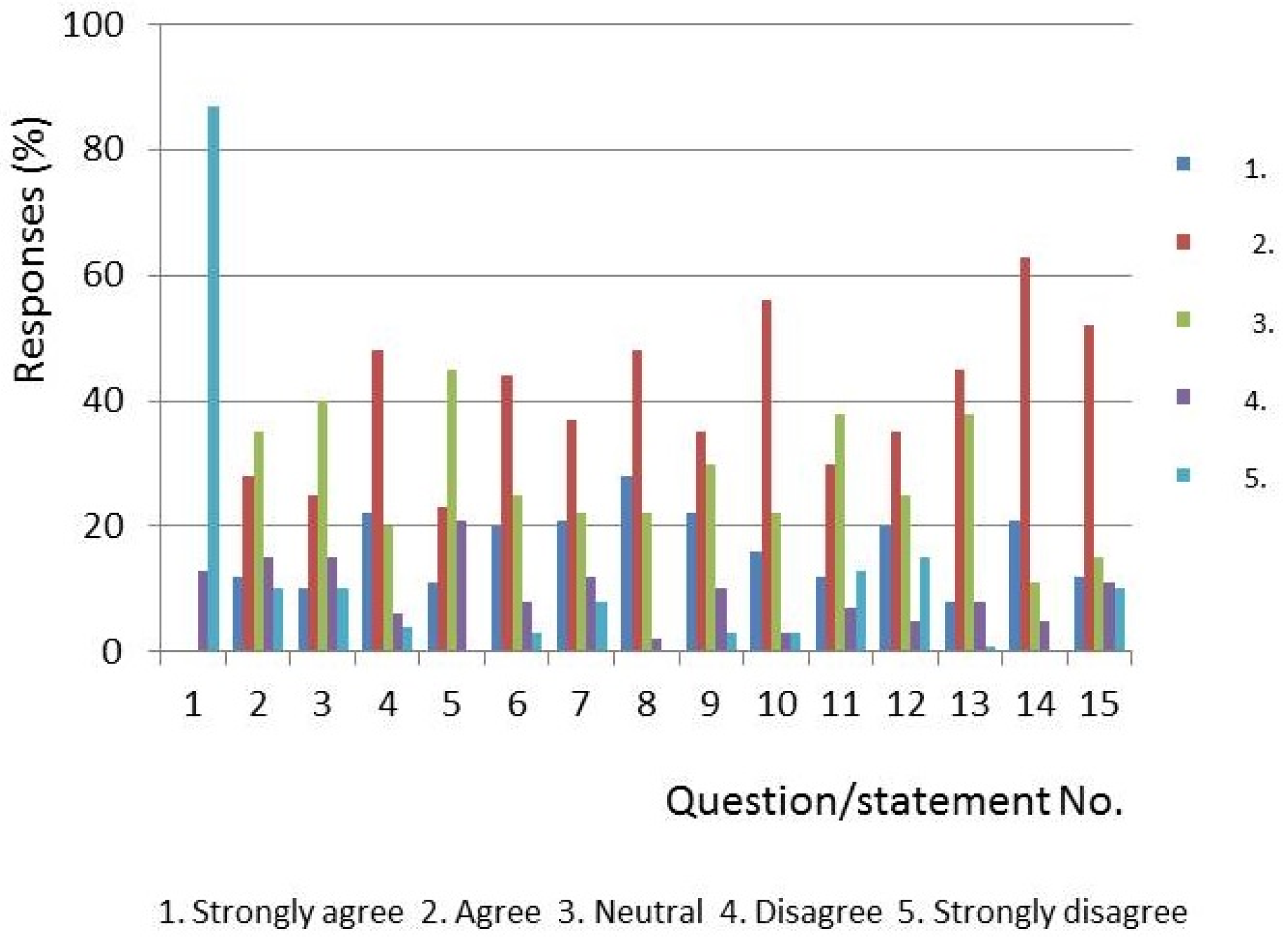
An anonymous online survey was conducted before students who had taken the course were given their final grades for the course to help with its formative evaluation. The fifteen questions/statements listed in
Table 2 were used during the survey, with each student requested to mark as they thought appropriate, on a five-point Likert scale, whether they: strongly agree, agree, neutral, disagree, strongly disagree with the question/statement. There was also a column to mark if they had no opinion, and a space to make short comments for qualitative feedback.
Generally, student feedback surveys have a very low response rate [
30,
31]. However the response rate here was relatively high (77%) and overall the results of the survey showed a positive attitude of the students towards the course. The numerical responses to the survey are shown on
Figure 9 and indicate that students felt they had benefited from their exposure to this CFD course. In additional comments made by the students the view was expressed that the amount of material introduce was about right, although some felt that some of the exercises were unnecessarily long. Students did not seem to worry about the concept of streamfunction being used but some did express concern about their understanding of vorticity in a physical sense. The students were generally appreciative that they could easily visualize flow using contour and vector plots and generally agreed that the combination of basic theory combined with computer coding gave them more confidence and understanding. Student showed some enthusiasm about learning more about CFD and in particular how they could incorporate CFD into projects from other subjects and capstone projects.
It was noted that the students liked the hands-on and self-discover approach, although at times some frustration was also noted, and they were fairly neutral on working in groups as opposed to working on their own. In fact it was very noticeable that students took pride in performing the simulations by themselves with a real sense of achievement ensuing.
Several points should also be made: the traditional view of CFD is that it has a steep learning gradient, but it has been shown here that with proper interfaces and a limited depth of flow difficulty that this gradient can be brought to an acceptable level. Also, it should be pointed out that for the practical software used no mention of code development was made to the students, as the learning outcome was to become proficient in the use of the existing coding. This would need to be remedied by a later course which involves ways of interacting with the existing, quite complicated core coding.
Evaluation of the course will continue in the future and hence be developed according to results. Only student views have been collected up to now but it is intended to take into account both student and instructor views in the future. It is felt more attention to how interest is aroused in general concerning the use of CFD is needed in future surveys as is the promotion of the use of CFD as a research tool during say capstone projects and post-graduate work. There will also be an attempt to elicit feedback from students who are at the ‘beyond-completion’ stage of the course.
5. Conclusions
In this paper the approach to delivering understanding of the numerical and practical aspects of the use of Navier-Stokes equations to solve fluid mechanics problems is outlined. For the numerical understanding, a well-defined sequence of steps needed to solve the Navier-Stokes equation cast in vorticity-streamfunction form was outlined. The sequence was integrated with the software package Mathematica at appropriate stages to take care of tedious computations, and hence allowed the students to concentrate on the overall details of the solution process. In addition, it is now important generally to integrate computer technology so as to complete and compliment lectures and theory. This has the advantages of helping with the computations, aiding presentation for reports and the ability to continue with further analysis as well as motivation for the students. Incorporating Mathematica also takes away the ‘black-box’ approach so often encountered by students with full CFD commercial codes, which give no real understanding of the numerical mathematics involved.
In addition to teaching the students some of the numerical aspects of CFD, this course also allowed for an introduction to the type of CFD carried out in professional offices, and taught additional topics like turbulence modelling, the idea of obtaining a grid independent solution and how critical it is to validate results obtained by the CFD approach. One of the main reasons for the inclusion of the second part of this course was to give the students practical skills and it was found that the simplified interface design does provide students with hands-on experience, gained through an interactive and user-friendly environment, and encourages student self-learning. It was noted from a survey that students liked getting hands-on experience and the self-discovery approach, although at times some frustration was noted when setting a problem up.


