Dynamics of an Ellipse-Shaped Meniscus on a Substrate-Supported Drop under an Electric Field

Department of Mathematical Sciences, New Jersey Institute of Technology, Newark, NJ 07102, USA
*
Author to whom correspondence should be addressed.
Fluids 2019, 4(4), 200; https://0-doi-org.brum.beds.ac.uk/10.3390/fluids4040200
Submission received: 1 October 2019
/
Revised: 12 November 2019
/
Accepted: 26 November 2019
/
Published: 29 November 2019
(This article belongs to the Special Issue Drop, Bubble and Particle Dynamics in Complex Fluids
)
Abstract
:The behavior of a conducting droplet and a dielectric droplet placed under an electric potential is analyzed. Expressions for drop height based on electrode separation and the applied voltage are found, and problem parameters associated with breakup and droplet ejection are classified. Similar to previous theoretical work, the droplet interface is restricted to an ellipse shape. However, contrary to previous work, the added complexity of the boundary condition at the electrode is taken into account. To gain insight into this problem, a two-dimensional droplet is addressed. This allows for conformal maps to be used to solve for the potential surrounding the drop, which gives the total upward electrical force on the drop that is then balanced by surface tension and gravitational forces. For the conducting case, the maximum droplet height is attained when the distance between the electrode and the drop becomes sufficiently large, in which case, the droplet can stably grow to about 2.31 times its initial height before instabilities occur. In the dielectric case, hysteresis can occur for certain values of electrode separation and relative permittivity.
1. Introduction
Electrified fluids appear in a wide variety of applications, such as inkjet printing [1,2,3], electrospray ionization/mass spectrometry [4,5], electrospinning [6,7], focused ion beam (FIB) technology [8,9], and nanotechnology [10]. However, an early motivation for Rayleigh and Taylor to study the behavior of droplets in electric fields came from nature, as electrified fluids play an important role in producing thunderstorms [11,12]. Many early theoretical papers by Taylor [11], and others, primarily focused on droplets suspended in uniform fields [13,14]. To analyze this problem, Taylor assumed that the interface was an ellipsoidal shape, derived a two-point approximation satisfying the Young-Laplace’s equation at the poles and equator of the ellipsoid, which resulted in an expression relating droplet height to the strength of the surrounding field. After Taylor’s original work on conducting drops in uniform fields, Miksis [15] extended Taylor’s approach to dielectric drops, and also performed numerical work which showed that hysteresis or bistability could occur for certain values of relative permittivity.
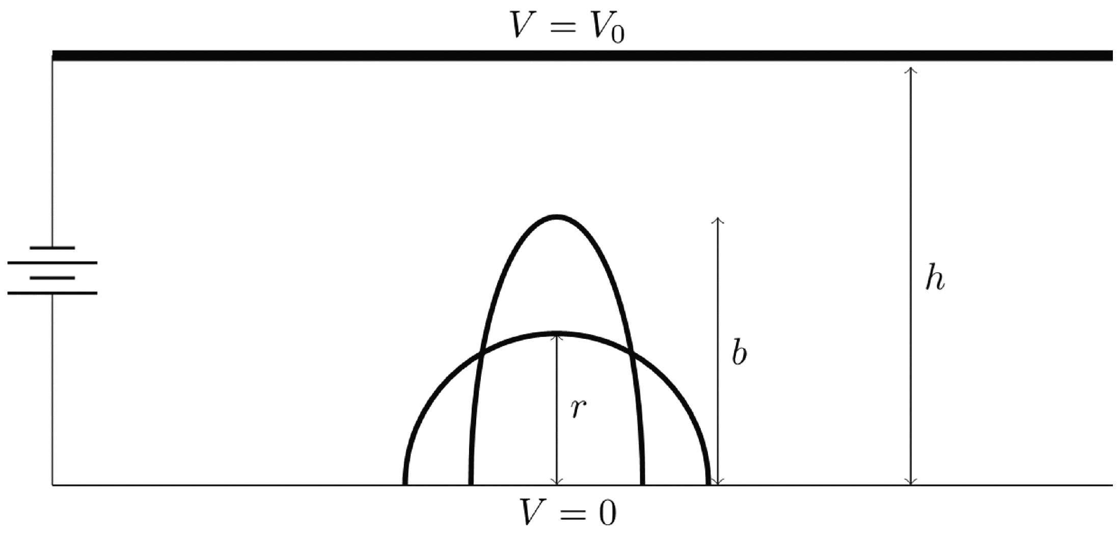
However, in many applications and experiments, an electric potential is placed directly above the droplet, and the electric field surrounding the drop is not uniform. This creates a new problem, which is sketched in Figure 1. Taylor and McEwan theoretically analyzed this problem, but instead of assuming an ellipsoidal shape and solving for the surrounding potential, they assumed that the interface was horizontal at its poles and guessed a potential that satisfied the upper boundary condition at the electrode [16]. Since then, Corson et al. [17,18] theoretically analyzed a conducting drop in the limiting case where the distance between the substrate and the electrode was large, and obtained asymptotic results which predicted drop height for small surrounding electric fields.
When a sessile drop on a substrate is placed under an electric potential difference between the substrate and an electrode above the drop, for sufficiently large potentials (where ellipsoidal shapes are no longer stable), the drop forms a conical shape known as the Taylor cone [11]. In [6], Yarin et al. showed that the Taylor cone which is a specific self-similar solution is not unique and that there could also exist nonself-similar solutions that do not admit a Taylor cone. The theory and numerical simulations of the jetting of the Taylor cone has been described in some recent papers, e.g., [19,20,21]. Recently, a study conducted by Elele et al. [22] sparked new interests in this problem, as it experimentally analyzed a dynamic Taylor cone and found three possible modes that the droplet could form depending on the applied voltage. The first mode happened for small voltages when the droplet took on an ellipsoidal shape and steadily rose as the applied voltage increased. Another mode happened for the largest applied voltages where strong instabilities such as droplet ejection arose. An intermediate mode happened for moderate voltages where the droplet would form a pointed protrusion and periodically rose to touch the electrode, and in this mode, a universal self symmetry independent of the applied voltage was observed [22]. This work served as an early motivation for us to study the behavior of an electrified droplet.
In this paper, we analyze a perfectly conducting drop and a dielectric drop to mathematically understand why droplet behavior in both cases is similar for large values of permittivity but drastically different for small values of permittivity, and why bistability only happens for in-between values of permittivity. We take the boundary condition at the electrode into account and derive formulas that signify when instabilities such as droplet ejection or droplet beak-up occur. To achieve this, we address the two-dimensional version of this problem. We assume that the droplet takes on an ellipse shape, which allows us to approximate the potential surrounding the droplet and obtain the total upward electrical force on the droplet that is then balanced by surface tension and gravitational forces. These assumptions describe a problem that is different from the one that has been experimentally studied in [12,17,22,23], and thus, our exact values for droplet height and applied voltage that are associated with droplet stability deviate slightly from those observed in experiments. However, our approach reasonably predicts the overall behavior of the drop and gives further insight into how droplet behavior changes as a function of the permittivity.
2. Conducting Drop
For the case of a perfectly conducting drop, we have that the potential surrounding the drop satisfying the Laplace’s equation,
with a Dirichlet boundary condition at the electrode,
a homogeneous Dirichlet boundary condition at the droplet interface, which we parameterize by t,
a homogeneous Neumann boundary condition far away from the interface,
and finally, we take advantage of the symmetry about the major axis of the ellipse and only analyze the part of the interface which corresponds to , which gives one extra homogeneous Neumann boundary condition on the y-axis,
To solve for , we use the conformal map defined by,
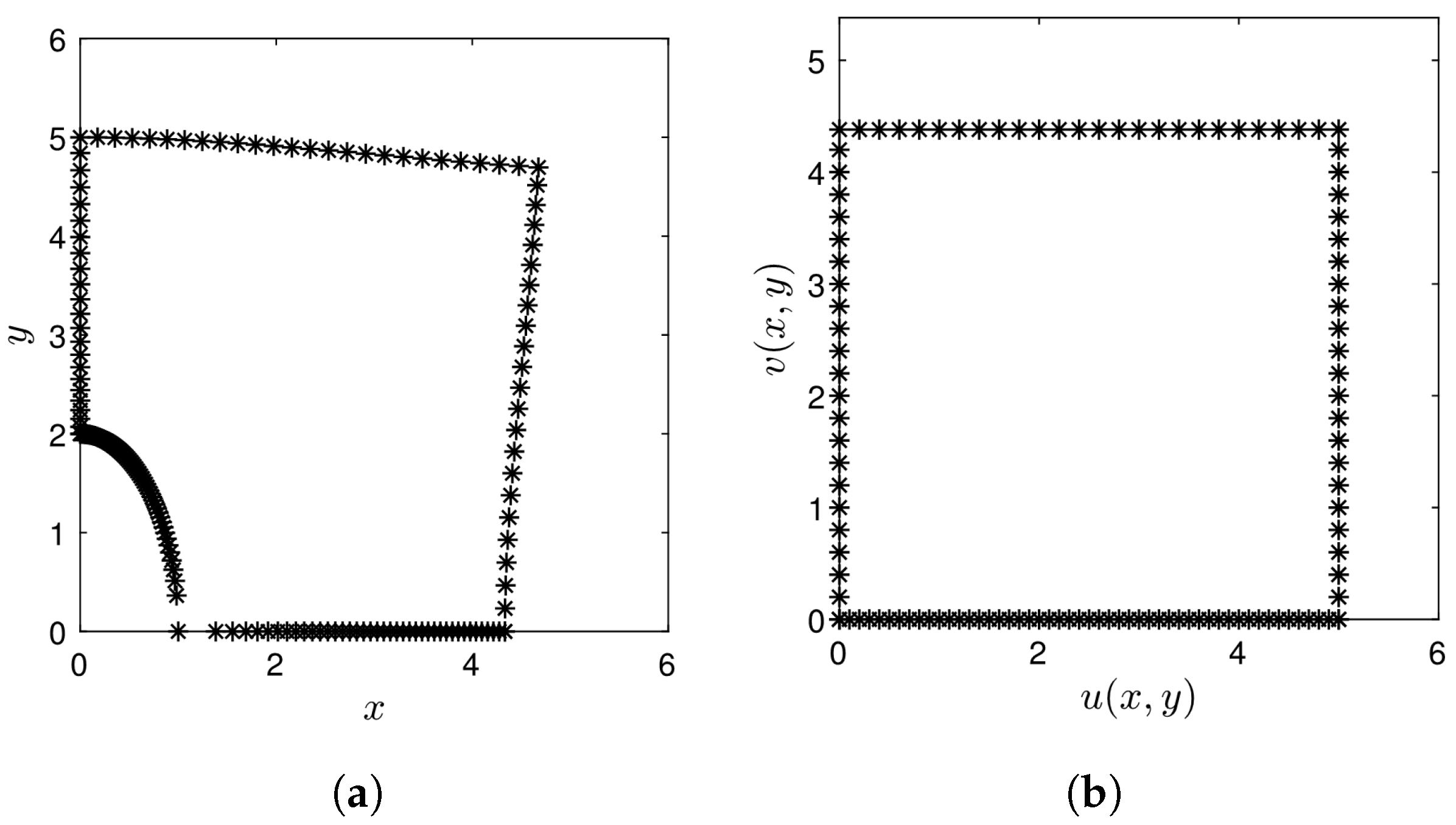
which maps a rectangle with height to a region that approximates the domain that we are working on (i.e., it maps the region on the right in Figure 2 to the region on the left), where
Thus, we have that the inverse of this map defined by,
will map a region which approximates our domain into a simple rectangle with height , which gives us the approximate surrounding potential,
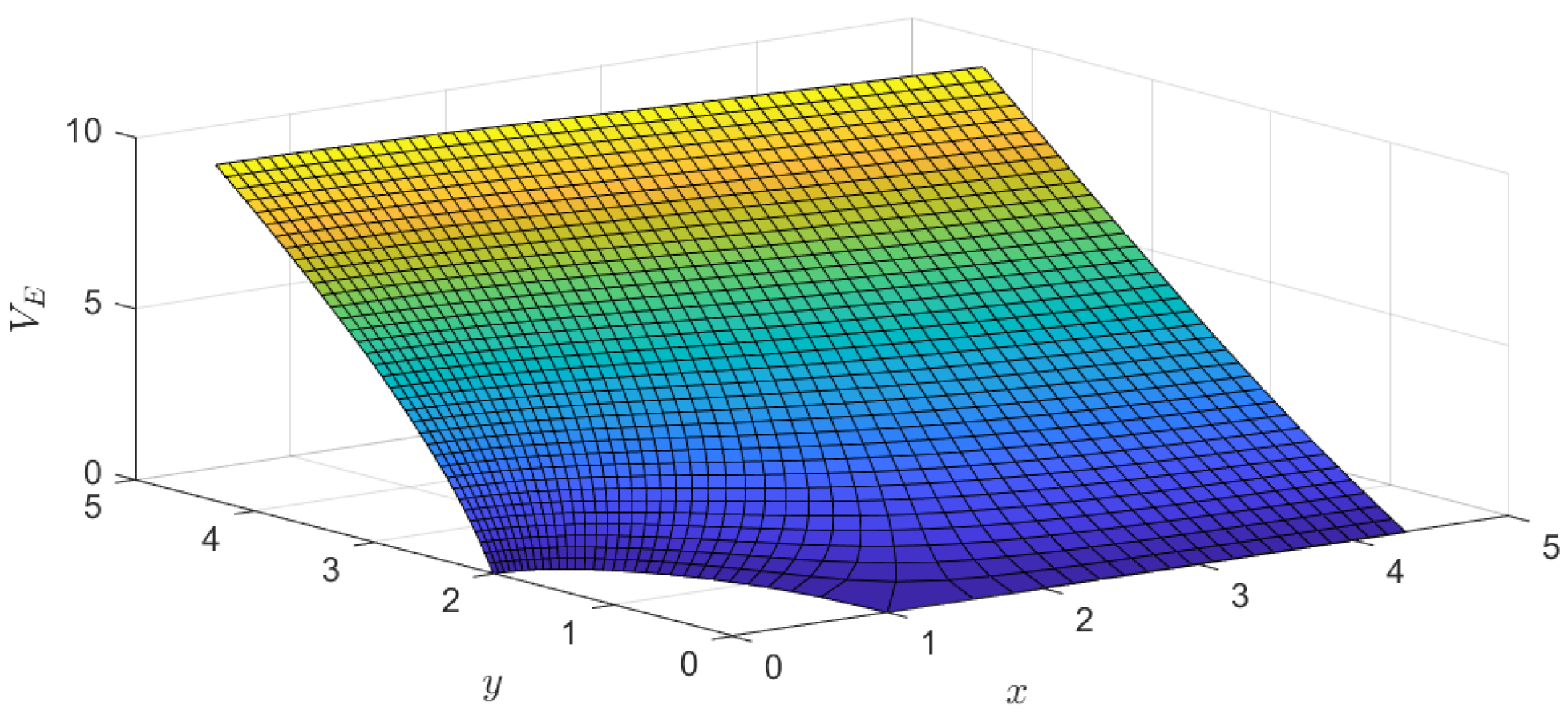
This gives the potential field shown in Figure 3 that is zero at the interface, and approximately linear far away from the interface.
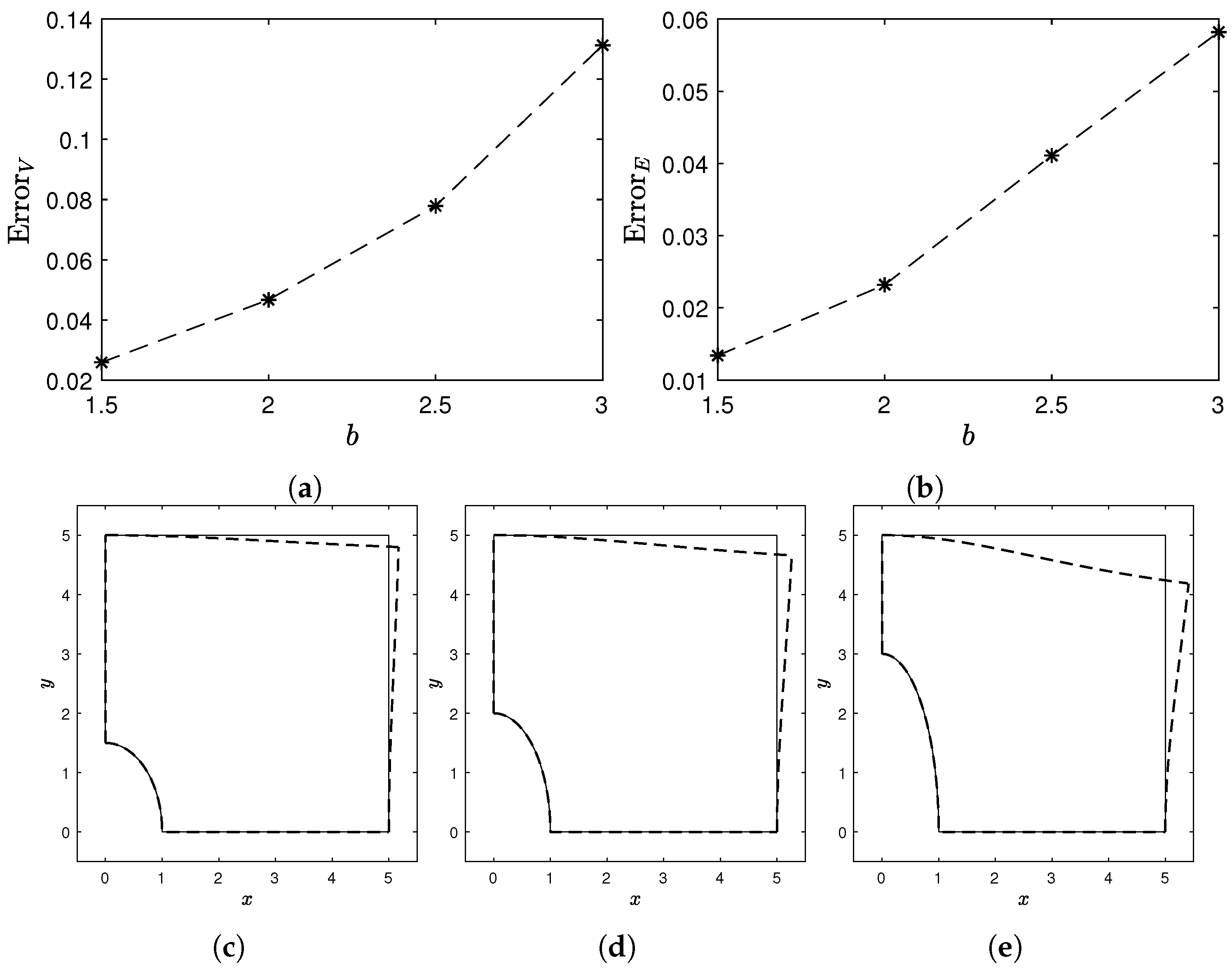
While the potential given above is not an exact solution to Equation (1) with the corresponding boundary conditions, as the boundary condition at the electrode is slightly warped, for most values of b and h the relative error at the interface is small. For instance, Figure 4a plots ErrorV for varying values of b where ErrorV is defined as
Here stands for a numerical finite element solution to Laplace’s equation on the exact domain, and the -norm is approximated by the function values at the grid points of the scheme. Furthermore, the error in the electric field at the interface which we define as
is plotted in Figure 4b for varying values of b (where stands for evaluated the interface). Both Figure 4a,b indicate that our analytical solution breaks down as b approaches h, as in this regime the top and right boundaries of our conformal mapped domain deviate from that of straight lines (see Figure 4c–e).
3. Total Force on the Conducting Drop
This gives a total electrical force per-unit area that is normal to the interface with magnitude given by,
where stands for evaluated at the interface, and is the permittivity of the medium surrounding the droplet [24,25]. In our case, this medium is air which means that . Setting and , we evaluate Equation (15) at the interface to get that
which gives the force distribution shown in Figure 5.
Integrating the expression given in Equation (16) and accounting for surface tension, pressure (we neglect the effect that the non-constant curvature of the ellipse has on the Laplace pressure and assume that the internal pressure is constant as in [11]), and gravitational forces dictates that the total upward force per-unit length on our cylindrical drop is,
Here r is the radius of the semi-circular drop, is the density of the fluid, is the surface tension constant, and g is the acceleration due to gravity. Assuming incompressibility of the liquid gives us , which allows us to express the total upward force per-unit length on the drop in terms of b.
Finally, we pick our characteristic length scale to be r and nondimensionalize Equation (17) to get that
where our new variables are
and
Our problem parameters are,
and
4. Results
Setting the total upward force on the droplet given in Equation (18) equal to zero gives us in terms of , R, and B. For simplicity, we set , and plot in terms of B for various values of electrode separation R. Similar to earlier analytical results by Taylor [11] and Miksis [15] for droplets in uniform fields and numerical results for the full three dimensional problem in [15,26,27], our method gives one stable branch of fixed points (solid line) and one unstable branch (dotted line). From Figure 6 which plots vs for varying values of R, we can see that our formula for two-dimensional drops, which takes into account electrode separation allows for larger drop heights and applied voltages than previous theoretical results for ellipsoidal drops by Miksis [15]. However, in Figure 6 we can also see that for small voltages our two dimensional approximation and Miksis’s [15] three dimensional approximation seem to agree well. Furthermore, from Figure 6, we have that for each value of R there is a certain threshold value of and a corresponding value of B which identifies the maximum stable height that the droplet can grow to. These threshold values are plotted in Figure 7, showing that a two-dimensional drop can only grow to its initial height before instabilities arise and that this maximum height happens when , and in the limiting case where or identically . This maximum value of deviates from Taylor’s analytical results in three dimensions which predict a maximum value of [11], and Taylor’s experiential results with thin films which predict a maximum value of [12]. However, our results are in agreement with experimental values in [22,23]. For instance, experiments by Macky [23] show that a free-falling drop in an electric field can grow to anywhere between and its original length before instabilities occur. Experiments done by Inculet and Kromann [28] on water droplets doped with alcohol and suspended in oil show that the droplet can stably grow to its initial height. Most recently, experiments done by Elele et al. [22] on electrified droplets on the International Space Station show that a droplet can stably grow to its original length. However, it is also important to note that in many of these experiments, the curvature at the tip of the droplet may be starting to deviate from that of an ellipse. Furthermore, this deviation from an ellipse shape might also be the reason why experiments give a voltage threshold that is higher than the one given by our method. For example, experiments carried out by Elele et al. [22] on a drop of slightly conducting water on Earth gravity with and an electrode separation of , found that the maximum voltage that could be applied before spontaneous shoot-up occurred was . However, our method predicts that for these problem parameters, the maximum voltage that can be applied before an ellipse is no longer a stable solution is . Nevertheless, in this case, gravitational forces are strong in comparison to the electrical forces, and because of this, electrode separation is quite small which means that the error in our calculated potential could also be having an effect.
5. Dielectric Drop
For the case of a dielectric drop, the boundary condition at the interface changes; instead of a Dirichlet boundary condition, we have a Neumann boundary condition at the interface, which specifies the jump in permittivity and is given by
Here is the unit normal vector of the interface, is the permittivity of the fluid, is the electric potential outside the droplet, and is the electric potential inside the droplet. Note that this boundary condition assumes that the fluid is a perfect dielectric and that no free charges build up at the interface [25].
Because we consider the potential inside the droplet, we cannot use the map given in Equation (8), so instead we use the map given by
which maps the rectangle with width and height to the region enclosed by the quarter of an Ellipse with major axis b and minor axis a. Furthermore, the horizontal line segment given by,
where , and
gets mapped to the region enclosed by the quarter of an ellipse with major axis h and minor axis (see Figure 8). From here, we can see that for most values of b, the width of this outer ellipse will be much bigger than a.
Thus, the inverse of this map, given by
will allow us to solve the desired equations on an elliptical annulus; however, this requires us to define a boundary condition on the outer ellipse. To ensure that this boundary condition is physically relevant and approximates the boundary condition at the electrode, we define on this outer ellipse to be equal to our conducting potential given in Equation (9). This turns out to be a good approximation for the boundary condition at the electrode, as we find that the error for our potential in the dielectric case is bounded by the error in the conducting case (results not show here).
Because we are only working in the first quadrant, we can define a branch of that is analytic everywhere on the elliptical annulus except at the point , . This branch of is defined by the branch of given by,
Using the fact that conformal maps preserve both the Laplace’s equation and homogeneous Neumann boundary conditions, we arrive at,
and,
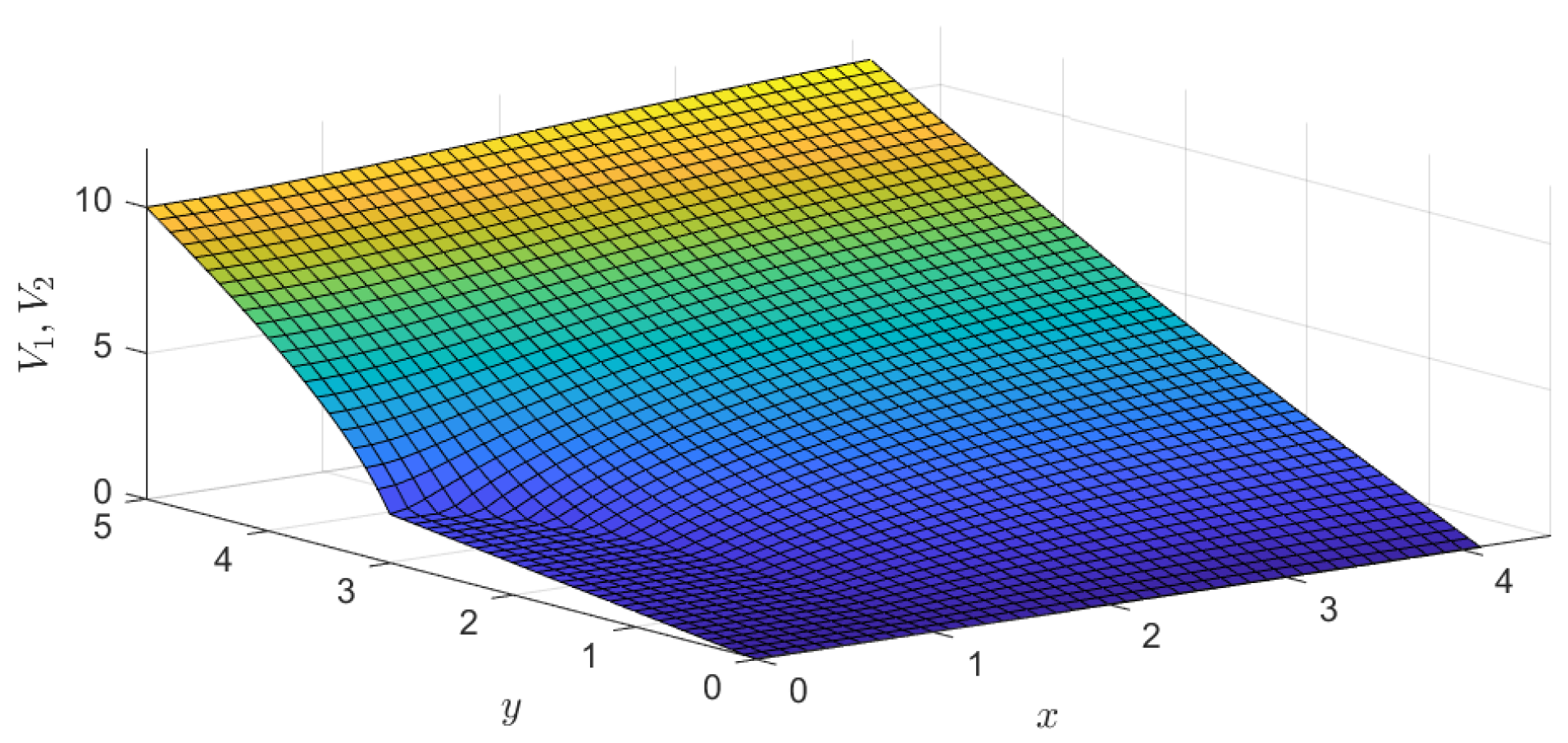
where X and Y are given by a branch of the inverse transformation. Here we notice that the potential inside the droplet is linear, which implies that the field in that region is uniform, and we can also see that the potential inside the droplet approaches zero as , which implies that in the limiting case where the permittivity of the drop goes to infinity goes to zero and goes to (the potential surrounding the conducting drop). Additionally, the example plot (Figure 9 ) of the potential given in Equations (30) and (31) shows that while the potential inside the droplet is linear, the potential directly outside the drop is nonlinear and approaches a linear function for values of x, and y that are large.
6. Total Force on the Dielectric Drop
Equation (30) gives the vertical electric field inside the droplet, defined by,
Equation (31) gives an electric field outside of the drop that has an x-component of,
and a y-component of,
This allows to calculate the total force exerted at interface, yielding
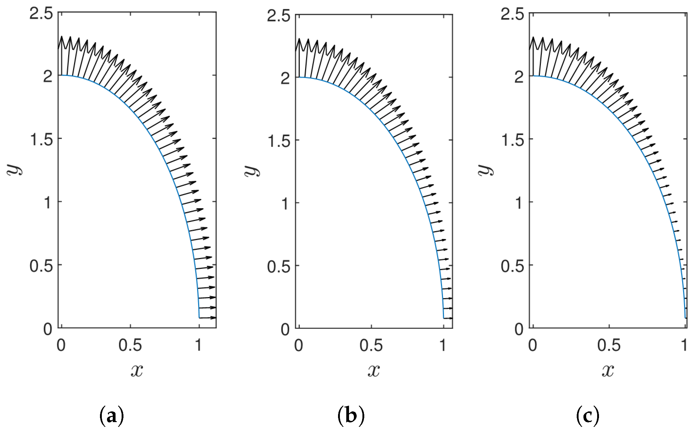
where is the normal electrical force per-unit area at the interface (note that since there are no free charges, the electrical force will be in the interface normal direction), and stands for the jump in at the interface [24,25]. The expression in Equation (35) gives the force distribution shown in Figure 10. From here, we observe that the electrical force distribution is almost uniform for small values of relative permittivity.
By integrating Equation (35) from 0 to , accounting for surface tension and gravitational forces, and non-dimensionalizing, we get that the total dimensionless force (see Equation (19)) on the droplet is,
where,
and
Equation (36), therefore, gives the total upward force on the droplet in terms of three non-dimensional parameters , , and R that are identical to that of the conducting case, and one new parameter
7. Results
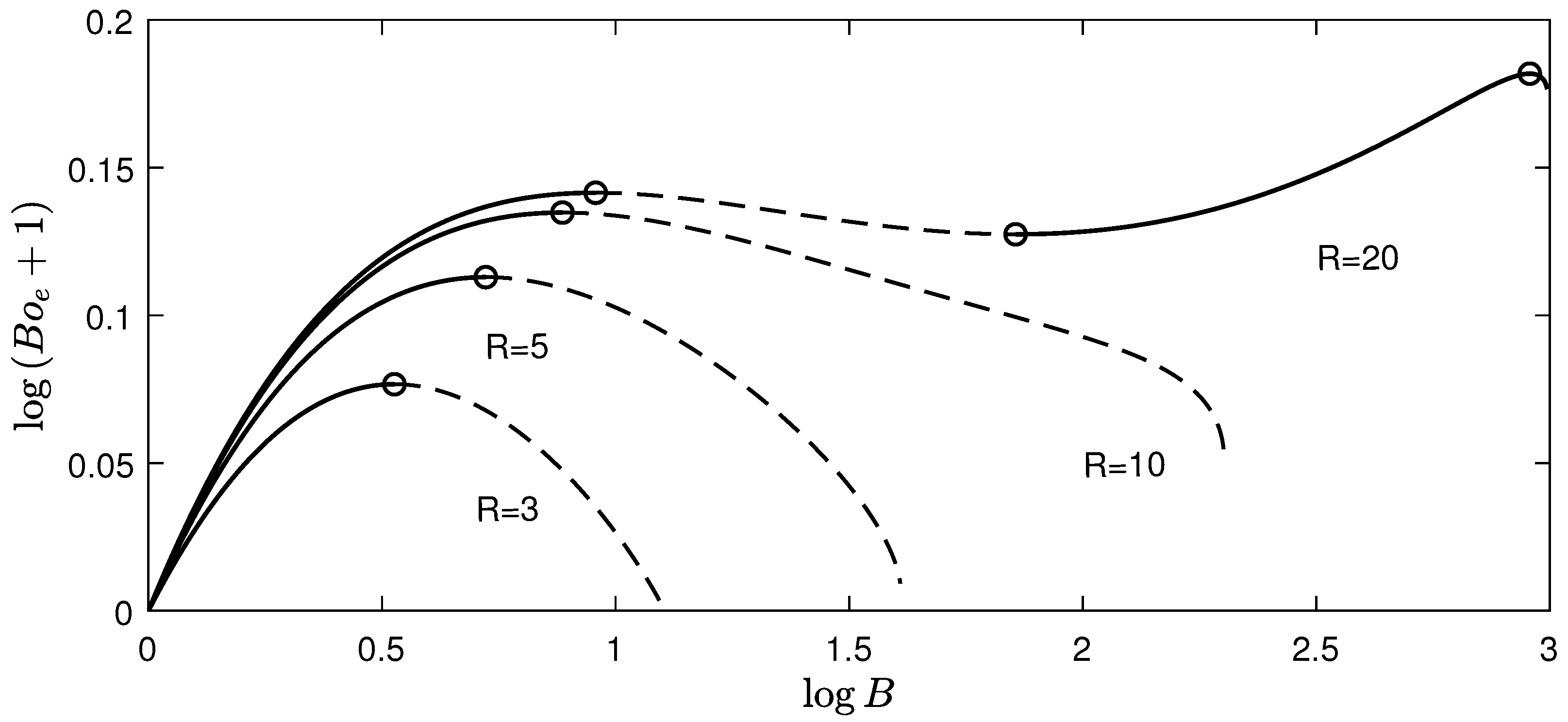
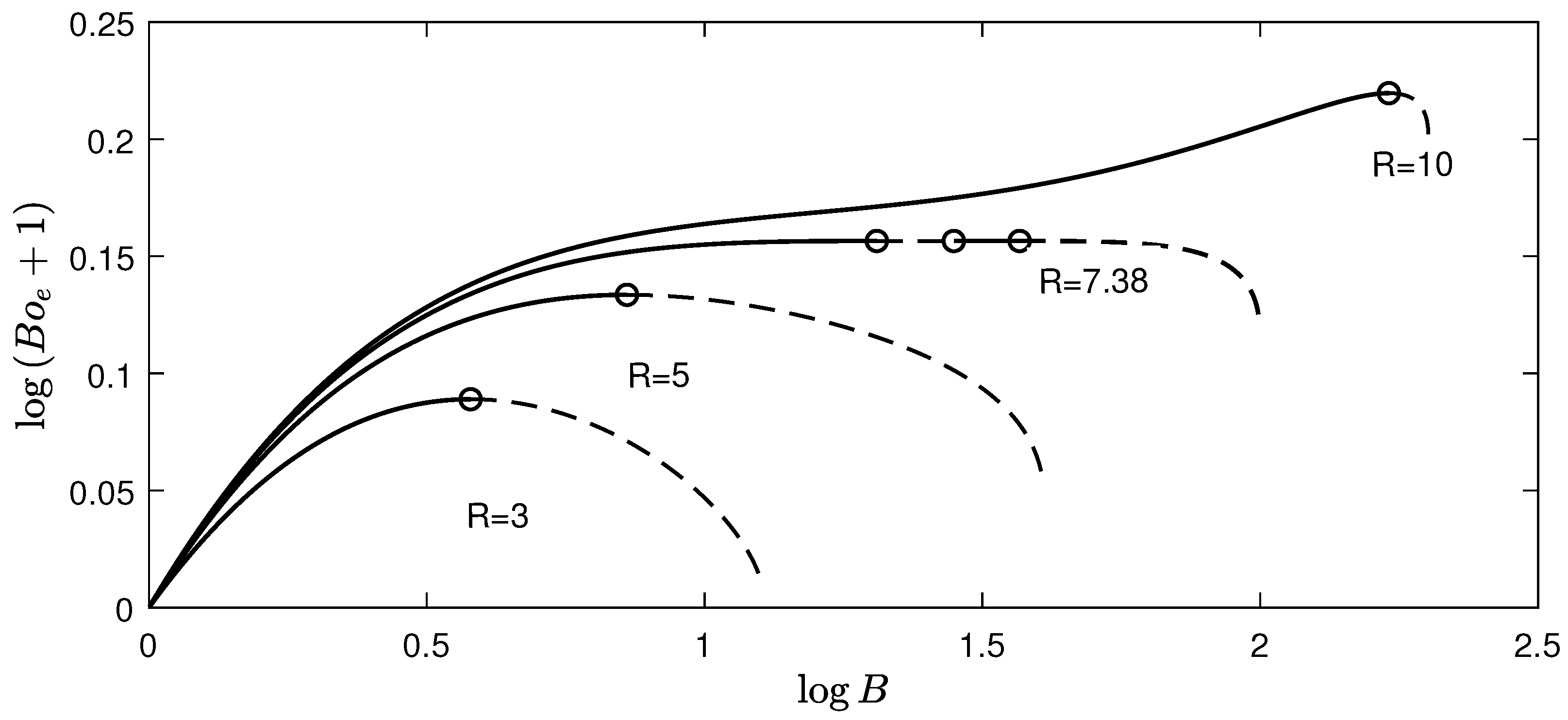
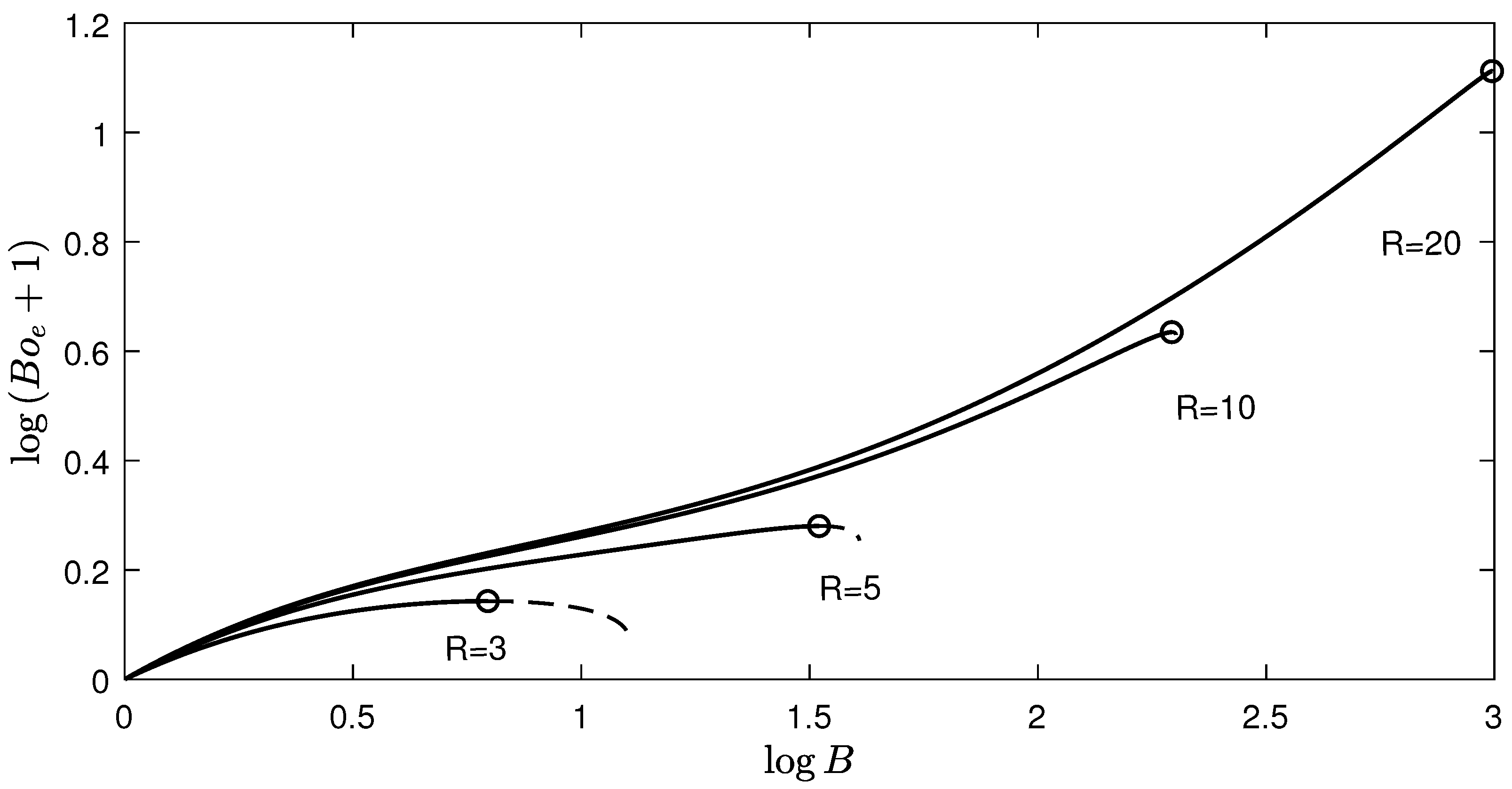
As before, we set the expression for total force given in Equation (36) equal to zero, which allows us to express in terms of B. This gives three different types of behavior based on the values of . In case one, where , and R is fixed we predict that the droplet behaves similarly to the conducting drop (see Figure 11). In case two, where we have that hysteresis or the presents of two stable branches of fixpoints can occur for certain values of R (see Figure 12). Finally, in the third case, where , a wide range of stable fixed points exists, which extends to just below the electrode (see Figure 13). The existence of two stable branches of fixed points for certain values of agrees well with numerical results for the three dimensional problem, as Ramos and Castellanos [27] and Wohlhuter and Basaran [26] predict a similar behavior, however, their minimum value for which hysteresis can occur is as opposed to our prediction of for the two dimensional problem.
8. Conclusions
Conformal maps are used to analyze the behavior of a substrate supported two-dimensional droplet that is placed under an electric potential. In both the conducting case and the dielectric case, the behavior of a two-dimensional droplet is similar to that of a three dimensional one. In the case of a conducting drop, we find that the maximum stable high for an ellipse shape droplet is , which has a corresponding voltage value of . In the dielectric case, we find that when problem parameters are fixed and permittivity is large, the potential surrounding a dielectric drop approaches the potential that surrounds a conducting drop, and thus a dielectric drop behaves similar to a conducting drop. However, in the intermediate range where the permittivity of the drop is above 29 but also not too large, we have that hysteresis can occur for certain values of electrode separation. Finally, when the permittivity of the drop is below 29 we have that the behavior of a dielectric drop is far different than that of a conducting drop, as a wide range of stable fixed points that rise to just below the electrode exists. In the future, we hope to apply this conformal map approach to address droplets with varying contact angles, and general droplets with interfaces that are not restricted to an ellipse.
Author Contributions
Formal analysis, P.Z.; methodology, S.A.; supervision, S.A.; visualization, P.Z.; writing—original draft, P.Z.; writing—review and editing, S.A.
Funding
This research received no external funding.
Acknowledgments
We acknowledge the partial support by the Petroleum Research Fund PRF-59641-ND and the NJIT Provost’s Summer Research Award.
Conflicts of Interest
The authors declare no conflict of interest.
References
- Jiang, H.; Tan, H. One dimensional Model for droplet ejection process in inkjet devices. Fluids 2018, 3, 28. [Google Scholar] [CrossRef]
- Bos, A.V.; Meulen, M.V.; Driessen, T.; Berg, M.; Reinten, H.; Wijshoff, H.; Versluis, M.; Lohse, D. Velocity profile inside piezoacoustic inkjet droplets in flight: Comparison between experiment and numerical simulation. Phys. Rev. Appl. 2014, 1, 014004. [Google Scholar]
- Eggers, J.; Villermaux, E. Physics of liquid jets. Rep. Prog. Phys. 2008, 71, 036601. [Google Scholar] [CrossRef]
- Gaskell, S.J. Electrospray: Principles and practice. J. Mass Spectrom. 1997, 32, 677–688. [Google Scholar] [CrossRef]
- Wilm, M.; Shevchenko, A.; Houthaeve, T.; Breit, S.; Schweigerer, L.; Fotsis, T.; Mann, M. Femtomole sequencing of proteins from polyacrylamide gels by nano electrospray mass spectrometry. Nature 1996, 379, 466–469. [Google Scholar] [CrossRef] [PubMed]
- Yarin, A.L.; Koombhongse, S.; Reneker, D.H. Taylor cone and jetting from liquid droplets in electrospinning of nanofibers. J. Appl. Phys. 2001, 90, 4836–4846. [Google Scholar] [CrossRef]
- Bhardwaj, N.; Kundu, S.C. Electrospinning: A fascinating fiber fabrication technique. Biotechnol. Adv. 2010, 28, 325–347. [Google Scholar] [CrossRef]
- Gierak, J. Focused ion beam technology and ultimate applications. Semicond. Sci. Tech. 2009, 24, 043001. [Google Scholar] [CrossRef]
- Matsui, S.; Ochiai, Y. Focused ion beam applications to solid state devices. Nanotechnology 1996, 7, 247–258. [Google Scholar] [CrossRef]
- Xie, J.; Lim, L.K.; Phua, Y.; Hua, J.; Wang, C. Electrohydrodynamic atomization for biodegradable polymeric particle production. J. Colloid Interface Sci. 2006, 302, 103–112. [Google Scholar] [CrossRef]
- Taylor, G.I. Disintegration of water drops in an electric field. Proc. R. Soc. A 1964, 280, 383–397. [Google Scholar]
- Wilson, C.T.R.; Taylor, G.I. The bursting of soap-bubbles in a uniform electric field. Math. Proc. Camb. Philos. Soc. 1925, 22, 728–730. [Google Scholar] [CrossRef]
- Cheng, K.J.; Chaddock, J.B. Deformation and stability of drops and bubbles in an electric field. Phys. Lett. A 1984, 106, 51–53. [Google Scholar] [CrossRef]
- Cheng, K.J.; Miksis, M.J. Shape and stability of a drop on a conducting plane in an electric Field. PhysicoChem. Hydrodynam. 1989, 11, 9–20. [Google Scholar]
- Miksis, M.J. Shape of a drop in an eletric field. Phys. Fluids 1981, 24, 1967–1972. [Google Scholar] [CrossRef]
- Taylor, G.I.; McEwan, A.D. The stability of a horizontal fluid interface in a vertical electric field. J. Fluid Mech. 1965, 22, 1–15. [Google Scholar] [CrossRef]
- Corson, L.T.; Tsakonas, C.; Duffy, B.R.; Mottram, N.J.; Sage, I.C.; Brown, C.V.; Wilson, S.K. Deformation of a nearly hemispherical conducting drop due to an electric field: Theory and experiment. Phys. Fluids 2014, 26, 122106. [Google Scholar] [CrossRef]
- Tsakonas, C.; Corson, L.T.; Sage, I.C.; Brown, C.V. Electric field induced deformation of hemispherical sessile droplets of ionic liquid. J. Electrostat. 2014, 72, 437–440. [Google Scholar] [CrossRef]
- Ganan-Calvo, A.M. On the theory of electrohydrodynamically driven capillary jets. J. Fluid Mech. 1997, 335, 165–188. [Google Scholar] [CrossRef]
- Lastow, O.; Balachandran, W. Numerical simulation of electrohydrodynamic (EHD) atomization. J. Electrostat. 2006, 64, 850–859. [Google Scholar] [CrossRef]
- Lauricella, M.; Melchionna, S.; Montessori, A.; Pisignano, D.; Pontrelli, G.; Succi, S. Entropic lattice boltzmann model for charged leaky dielectric multiphase fluids in electrified jets. Phys. Rev. E 2018, 97, 033308. [Google Scholar] [CrossRef]
- Elele, E.O.; Shen, Y.; Pettit, D.R.; Khusid, B. Detection of a dynamic cone-shaped meniscus on the surface of fluids in electric fields. Phys. Rev. Lett. 2015, 114, 054501. [Google Scholar] [CrossRef]
- Macky, W.A. Some investigations on the deformation and breaking of water drops in strong electric fields. Proc. R. Soc. A 1931, 133, 565–587. [Google Scholar] [CrossRef]
- Castellanos, A.; Gonzalez, A. Nonlinear electrohydrodynamics of free surfaces. IEEE Trans. Dielectr. Electr. Insul. 1998, 5, 334–343. [Google Scholar] [CrossRef]
- Hua, J.; Lim, L.K.; Wang, C.H. Numerical simulation of deformation/motion of a drop suspended in viscous liquids under influence of steady electric fields. Phys. Fluids 2008, 20, 113302. [Google Scholar] [CrossRef]
- Wohlhuter, F.K.; Basaran, O.A. Shapes and stability of pendant and sessile dielectric drops in an electric field. J. Fluid Mech. 1992, 235, 481–510. [Google Scholar] [CrossRef]
- Ramos, A.; Castellanos, A. Equilibrium shapes and bifurcation of captive dielectric drops subjected to electric fields. J. Electrostat. 1994, 33, 61–86. [Google Scholar] [CrossRef]
- Inculet, I.I.; Kromann, R. Breakup of large water droplets by electric fields. IEEE Trans. Ind. Appl. 1989, 25, 945–948. [Google Scholar] [CrossRef]
Figure 1.
Two-dimensional sketch of the problem. The initial radius of the cylindrical drop is given by r, the distance between the substrate and the electrode by h, the applied voltage by , and the new height of the drop with the applied voltage by b.
Figure 1.
Two-dimensional sketch of the problem. The initial radius of the cylindrical drop is given by r, the distance between the substrate and the electrode by h, the applied voltage by , and the new height of the drop with the applied voltage by b.

Figure 2.
The map given in Equation (6) maps from (b) to (a), and the inverse map given in Equation (8)
maps in the opposite direction.

Figure 3.
Example of the plot of the potential given in Equation (9) for , , and .
Figure 3.
Example of the plot of the potential given in Equation (9) for , , and .

Figure 4.
(a) The relative error between our analytical potential given in Equation (9) and a finite element solution for the potential on the exact domain, which we define as ErrorV (see Equation (10)) is potted for varying values of b. (b) The relative error in the electric field strength at the droplet interface given by our analytical solution (see Equation (12)) and a finite element solution on the exact domain, which we define as ErrorE (see Equation (11)) is plotted for varying values of b. (c–e) The exact domain (━) is plotted against our approximate conformal mapped domain (┅) for b = 1.5, b = 2, and b = 3. (a–e) We fix h to 5 and a to 1.

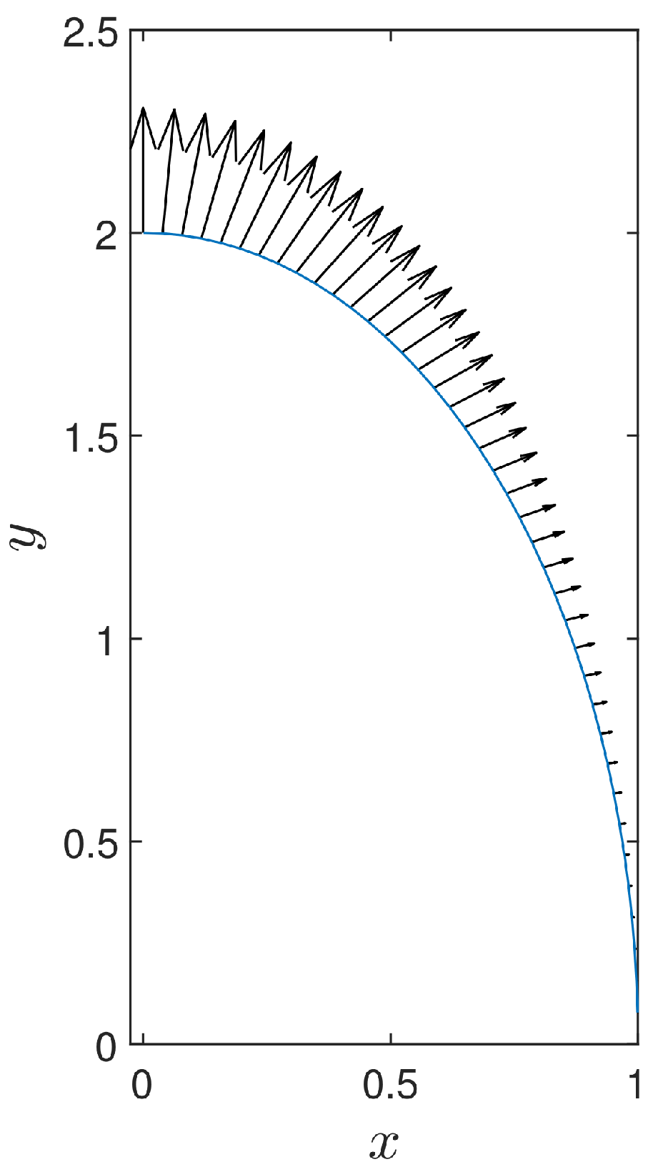
Figure 5.
Electrical force distribution around a conducting drop.

Figure 6.
Electrical bond number is plotted against B on a log- log scale for , , , and (━,┅), and values of obtained from Miksis’s [15] generalization of Taylor’s two point method for 3-dimensional ellipsoidal droplets in uniform electric fields is also plotted ( ![Fluids 04 00200 i001]() ). Here we can see that the stable branch of fixed points approaches a fixed curve as , while the unstable branch of fixed points reaches all the way to R, which corresponds to unstable drop heights that approach the height of the electrode.
). Here we can see that the stable branch of fixed points approaches a fixed curve as , while the unstable branch of fixed points reaches all the way to R, which corresponds to unstable drop heights that approach the height of the electrode.
 ). Here we can see that the stable branch of fixed points approaches a fixed curve as , while the unstable branch of fixed points reaches all the way to R, which corresponds to unstable drop heights that approach the height of the electrode.
Figure 6.
Electrical bond number is plotted against B on a log- log scale for , , , and (━,┅), and values of obtained from Miksis’s [15] generalization of Taylor’s two point method for 3-dimensional ellipsoidal droplets in uniform electric fields is also plotted ( ![Fluids 04 00200 i001]() ). Here we can see that the stable branch of fixed points approaches a fixed curve as , while the unstable branch of fixed points reaches all the way to R, which corresponds to unstable drop heights that approach the height of the electrode.
). Here we can see that the stable branch of fixed points approaches a fixed curve as , while the unstable branch of fixed points reaches all the way to R, which corresponds to unstable drop heights that approach the height of the electrode.
). Here we can see that the stable branch of fixed points approaches a fixed curve as , while the unstable branch of fixed points reaches all the way to R, which corresponds to unstable drop heights that approach the height of the electrode.
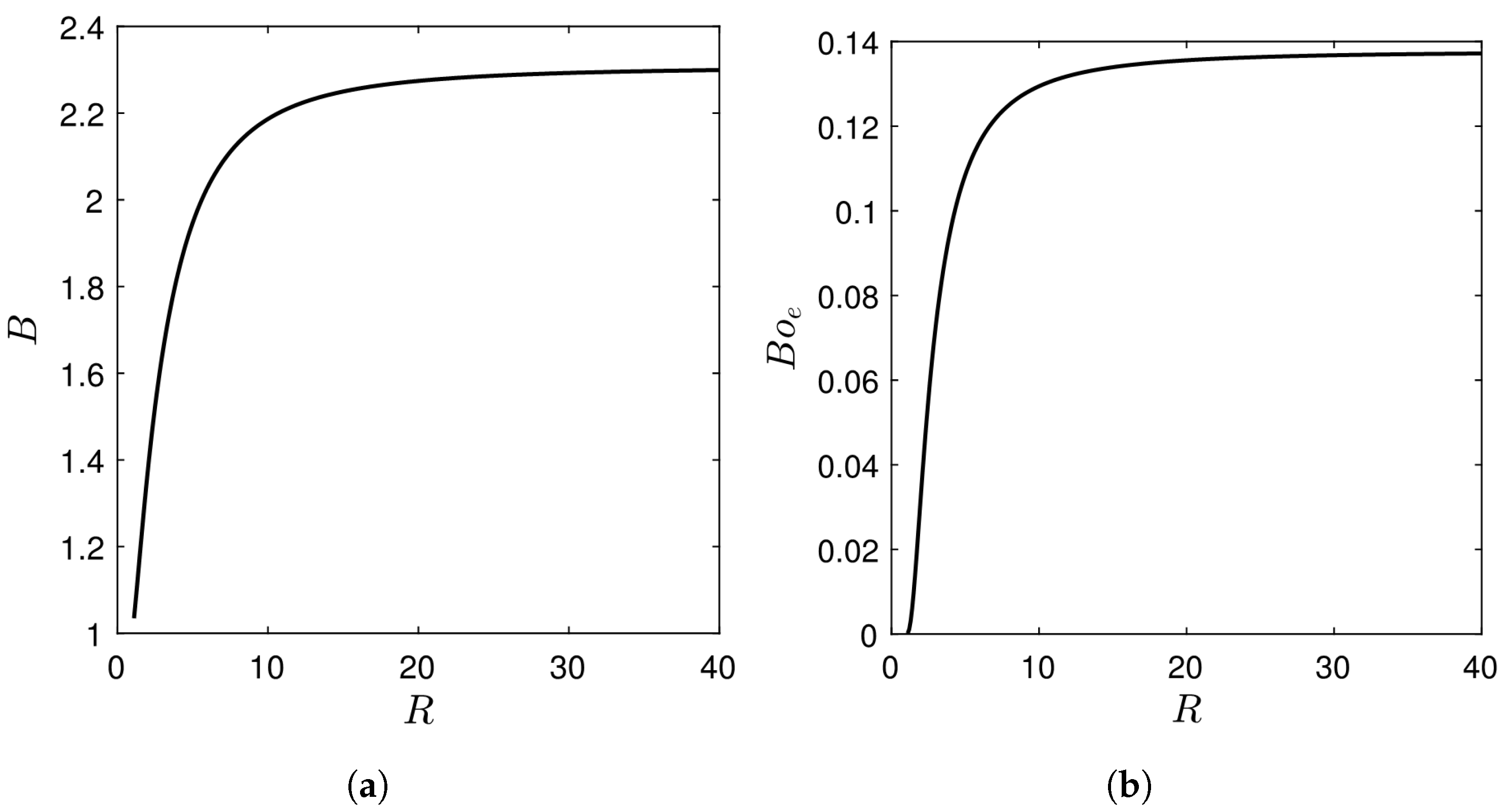
Figure 7.
(a) For each value of electrode separation (R), the maximum height that the droplet can stably achieve is plotted. (b) For each value of electrode separation (R), the applied potential (Boe) associated with this maximum height is plotted.
Figure 7.
(a) For each value of electrode separation (R), the maximum height that the droplet can stably achieve is plotted. (b) For each value of electrode separation (R), the applied potential (Boe) associated with this maximum height is plotted.

Figure 8.
Example of the map given in Equation (25) and the branch of its inverse define by Equations (28) and (29) for b = 3, a = , and h = 5. Here f(z) maps from (b) to (a).

Figure 9.
Example plot of the potential for the dielectric case when , , , and .

Figure 10.
Electrical force distribution around the dielectric drop for (a) ϵ = 5, (b) ϵ = 10, (c) ϵ = 50.
Figure 10.
Electrical force distribution around the dielectric drop for (a) ϵ = 5, (b) ϵ = 10, (c) ϵ = 50.

Figure 11.
as a function of B on a log-log scale for (which approximates the relative permittivity of water). We can see that for values of R that are small in comparison to , the droplet behaves similarly to a conducting droplet.
Figure 11.
as a function of B on a log-log scale for (which approximates the relative permittivity of water). We can see that for values of R that are small in comparison to , the droplet behaves similarly to a conducting droplet.

Figure 12.
as a functions of B on a log-log scale for , which is close to the minimum value of for which hysteresis can occur. We see that hysteresis can only happen for a small range of R values.
Figure 12.
as a functions of B on a log-log scale for , which is close to the minimum value of for which hysteresis can occur. We see that hysteresis can only happen for a small range of R values.

Figure 13.
as a functions of B on a log-log scale for , we see that for small values of a large range of stable fixed points exist, and the two-dimensional droplet can stably approach the electrode.
Figure 13.
as a functions of B on a log-log scale for , we see that for small values of a large range of stable fixed points exist, and the two-dimensional droplet can stably approach the electrode.

© 2019 by the authors. Licensee MDPI, Basel, Switzerland. This article is an open access article distributed under the terms and conditions of the Creative Commons Attribution (CC BY) license (http://creativecommons.org/licenses/by/4.0/).
Share and Cite
MDPI and ACS Style
Zaleski, P.; Afkhami, S. Dynamics of an Ellipse-Shaped Meniscus on a Substrate-Supported Drop under an Electric Field. Fluids 2019, 4, 200. https://0-doi-org.brum.beds.ac.uk/10.3390/fluids4040200
AMA Style
Zaleski P, Afkhami S. Dynamics of an Ellipse-Shaped Meniscus on a Substrate-Supported Drop under an Electric Field. Fluids. 2019; 4(4):200. https://0-doi-org.brum.beds.ac.uk/10.3390/fluids4040200
Chicago/Turabian StyleZaleski, Philip, and Shahriar Afkhami. 2019. "Dynamics of an Ellipse-Shaped Meniscus on a Substrate-Supported Drop under an Electric Field" Fluids 4, no. 4: 200. https://0-doi-org.brum.beds.ac.uk/10.3390/fluids4040200