Suite-CFD: An Array of Fluid Solvers Written in MATLAB and Python


Department of Mathematics and Statistics, The College of New Jersey, 2000 Pennington Road, Ewing Township, NJ 08628, USA
Fluids 2020, 5(1), 28; https://0-doi-org.brum.beds.ac.uk/10.3390/fluids5010028
Submission received: 1 October 2019
/
Revised: 6 February 2020
/
Accepted: 19 February 2020
/
Published: 25 February 2020
(This article belongs to the Special Issue Teaching and Learning of Fluid Mechanics)
Abstract
:Computational Fluid Dynamics (CFD) models are being rapidly integrated into applications across all sciences and engineering. CFD harnesses the power of computers to solve the equations of fluid dynamics, which otherwise cannot be solved analytically except for very particular cases. Numerical solutions can be interpreted through traditional quantitative techniques as well as visually through qualitative snapshots of the flow data. As pictures are worth a thousand words, in many cases such visualizations are invaluable for understanding the fluid system. Unfortunately, vast mathematical knowledge is required to develop one’s own CFD software and commercial software options are expensive and thereby may be inaccessible to many potential practitioners. To that extent, CFD materials specifically designed for undergraduate education are limited. Here we provide an open-source repository, which contains numerous popular fluid solvers in (projection, spectral, and Lattice Boltzmann), with full implementations in both MATLAB and Python3. All output data is saved in the format, which can be visualized (and analyzed) with open-source visualization tools, such as VisIt or ParaView. Beyond the code, we also provide teaching resources, such as tutorials, flow snapshots, measurements, videos, and slides to streamline use of the software.
Keywords:
fluid dynamics education; applied mathematics education; computational fluid dynamics; fluids visualization; open-source CFD; projection method; spectral fluid solver; Lattice Boltzmann Method; cavity flow; circular flow; interacting vortices; flow past cylinder; flow past porous cylinder; MATLAB; Python1. Introduction
Computational Fluid Dynamics (CFD) models are being applied to problems across all sciences and engineering. From designing more aerodynamic sportswear and vehicles, to understanding animal locomotion, to personalized medicine, to disease transmission, and to predicting hurricanes and atmospheric phenomena, it is difficult to find situations where greater knowledge of the underlying fluid dynamics isn’t desired or valuable. Due to its immense importance, many scientists have dedicated their careers to the field, whether they study particular fluid phenomena or develop tools, either experimental or numerical, for other scientists and engineers to use. Possibly because of how vital understanding fluid dynamics is to human flourishing, proving existence, uniqueness, and the possible breakdown of solutions to the system of non-linear partial differential equations that govern fluid dynamics is one of the Millennium Problems, to which the Clay Institute offers a 1 million dollar prize for solving [1]. On the other hand, CFD allows us to solve these equations, the Navier-Stokes equations, which are the equations that detail the conversation of momentum and mass for a fluid. For an incompressible, viscous fluid, they can be written as follows,
where and are the fluid’s velocity and pressure, respectively. The physical properties of the fluid are given by and , its density and dynamic viscosity, respectively. The independent variables are the time, t, and spatial position, . Here all variables that pertain to the fluid, e.g., and p, are written in an Eulerian framework on a fixed Cartesian mesh, . Think of a fixed Cartesian mesh as a rectangular grid to which over the course of the simulation physical quantities, like velocity, pressure, etc., are measured at specific lattice points. In an Eulerian framework, specific blobs of fluid are not tracked over time, as though they are billiard balls, but rather, we focus on measuring quantities of interest at specific locations in space, located on a fixed grid. Note that Equations (1) and (2) provide the conservation of momentum and mass, respectively.
Many techniques have been developed to solve the above system of equations, such as projection methods [2,3,4,5,6], spectral methods [7,8,9], and Lattice Boltzmann methods [10,11,12]; however, they are typically left out of undergraduate curricula due to the mathematical background required for implementation, while they are commonly found in graduate curricula [13]. Moreover, it is not only mathematical knowledge that is a barrier; CFD requires expertise in at least four knowledge domains [14]: flow physics, numerical methods, computer programming, and validation, either experimental or theoretical. Thankfully, this has not stopped academics from developing and researching methods to integrate CFD into undergraduate courses [13,14,15,16,17,18,19,20,21]. Some have offered best practices guides and advice for future CFD undergraduate courses [13,21]. Stern et al. [13] has suggested for beginners to focus on the overall CFD process and flow visualizations, in order to solidify their fundamental understanding of fluid physics. Appropriate flow visualizations also help students validate and verify their simulations through careful inspection [21].
As computer literacy is rapidly becoming more of a central focus in undergraduate curricula, CFD could be a natural outlet where students may not only implement and test algorithms, but also practice proper data analysis and data visualization, while building computational experience. Much of the fluid dynamics software that has been used in previous courses is either foreign to students or only commercially available [14,17,19,20]. Commercial software has been recommended by the American Physical Society and American Association of Physics Teachers as a tool to help students prepare for 21st century careers by exposing them to a greater range of experiences and opportunities [22,23]. Unfortunately due to expensive software licenses, some schools, particularly smaller institutions, may not be able to afford such software, especially if they would only be used intermittently to complement the existing course material.
Recently, popular programming languages selected for many undergraduate curricula in science, mathematics, and engineering have been either MATLAB or Python [24,25,26,27,28]. MATLAB [29] and Python [30] are both interpreted languages, making it easier (and more attractive) for students to begin programming [31]. Moreover if students have already been exposed to these programming languages, giving them a platform to refine their skills in these languages while at the same strengthening their intuition in fluid dynamics may prove beneficial.
For this reason, many scientists, engineers, and mathematicians who are passionate about education have begun developing CFD software intended for educational purposes written in these languages [32,33,34,35,36]. Such open source software packages can be integrated into courses in a well-streamlined fashion, with tutorials, activities, exercises, and notes provided, and may even blur the line between classroom activities and contemporary research [32,35,36,37]. In particular L.A. Barba and G. Forsyth [33] have developed a guide for students to numerically solve the Navier-Stokes equations in 12 scaffolding steps and L.A. Barba and O. Mesnard [34] have developed a similar scaffolding lesson structure for students to study classical aerodynamics using potential flow models. Both are written in Python using Jupyter Notebooks [38]. Pawar and San [39] developed modules for teaching advanced undergraduate and graduate students how to develop their own fluid solvers in the Julia programming language [40].
Rather than develop a collection of modules that teach how to implement particular CFD numerical schemes, we offer the scientific community a variety of popular fluid solvers that solve traditional problems in fluid dynamics, with two independent but equal implementations written in MATLAB and Python. The emphasis is not placed on students having to develop or implement numerical schemes, but to allow them the opportunity to get an accelerated start in CFD, and run, tweak, and analyze simulations of traditionally studied problems in fluids courses, as well as explore data visualization and how to present data that is appropriate for fluid physics interpretation. All of this can be done while testing their own hypotheses in familiar programming environments. In the remainder of this manuscript, we will give a high-level overview of the CFD schemes currently implemented in the software (Section 2), guided tutorials on how to run, visualize, and analyze simulations (Section 3), and provide numerous examples to which students may elect to study or modify as well (Section 4).
Furthermore, we provide an in-depth mathematical description of each numerical scheme in Appendix B. The open-source software repository can be accessed at https://github.com/nickabattista/Holy_Grail. Any simulation data produced from the software can be visualized and analyzed in open-source software, such as VisIt [41], maintained by Lawrence Livermore National Laboratory, or ParaView [42], developed by Kitware, Inc., Los Alamos National Laboratory, and Sandia National Labs. We also provide teaching resources, such as slides, figures, and movies in the Supplementary Materials.
2. Brief Overview of the Three Fluid Solvers
In this section we will give a brief overview of the three fluid solvers currently implemented in the software—a projection method, a spectral (FFT) method, and the Lattice-Boltzmann method. Our goal is to provide students a high-level overview of the methods and how they compare to one another. Further details regarding their mathematical foundations and implementations are given in Appendix B.
2.1. Projection Method
The projection method was first introduced by Chorin in 1967 [2] and independently by Temam in 1968 [4], to solve the viscous, incompressible Navier-Stokes equations. Projection methods are finite difference based numerical schemes [43], in which the fluid equations are solved in an Eulerian framework, i.e., the computational grid is static and fluid dynamics variables, like velocity, pressure, etc., are measured at particular locations on the grid over time during a simulation. Projection methods have been extensively used throughout the fluid dynamics community for decades, in numerous applications across many fields, while being continually improved for efficiency and accuracy [5,44,45,46].
In a nutshell, this method decouples the velocity and pressure fields, using operator splitting and a Helmholtz-Hodge decomposition. This makes it possible to explicitly solve Equations (1) and (2) in a few steps [2] while also increasing computational efficiency. Please see Appendix B.1 for further mathematical details.
Furthermore, projection methods allow one to define explicit boundary conditions (BCs) for velocity on edges of the computational domain, whether they are Dirichlet, Neumann, or Robin boundary conditions [5,47]. In our software, we allow users to impose tangential velocity boundary conditions along the edges of the rectangular domain, while the normal direction boundary conditions for velocity are explicitly set to zero. The choice to set normal BCs to zero was made in order to simplify the code by ensuring that volume conservation would be automatically satisfied, i.e., situations will not arise in which a specified amount of fluid is being pumped into the domain while a different amount is leaving the domain per unit time.
Having defined the fluid velocity as , one can set the boundary conditions for u on the top and bottom of the domain ( along these edges) or v on the left and right sides ( along these edges). See Figure 1 for an illustration. Later in Section 4, we will showcase two different traditional problems in fluid dynamics with a projection method:
- Cavity Flow
- Circular Flow in a Square Domain
The examples are different due to the changes in boundary conditions that the user can impose, see Figure 1. In Figure 1 we illustrate the boundary conditions for each example: cavity flow (a) and circular flow (b). This figure also illustrates that the domain could be constructed to be either rectangular or square and that the boundary conditions do not have to be uniform among all sides, nor across the domain.
We will also compare different fluid scales in both examples, using the Reynolds Number, . The Reynolds Number is given by
where and are the fluid’s density and dynamic viscosity, respectively, while L and V are a characteristic length- and velocity-scale of the system. In essence, is a ratio of inertial forces to viscous forces in a system. If , inertia dominates, if , viscous forces dominate, and if , the inertia and viscous forces are balanced. An example of high flow would be the flow around a marble quickly falling through air. An example of low flow would be the fluid flow around a marble slowly falling through honey.
2.2. Spectral Method (FFT)
Spectral methods are a different class of differential equation solvers. They are well-known for achieving highly accurate solutions, i.e., spectral accuracy [48,49,50]. Spectral accuracy occurs when error decreases exponentially with a small change in grid resolution, e.g., there is a linear relationship between the logarithm of error and grid resolution, i.e.,
where N is the number of grid points. These methods approximate solutions using orthogonal expansions, such as Fourier Series or other orthogonal basis of functions, like Chebyshev Polynomials or Legendre Polynomials. In contrast to finite difference based schemes, like the projection method, where solutions are approximated at specific locations in space, in spectral methods a particular orthogonal series expansion is chosen and the earnest is on finding the coefficients of the expansion.
Here we chose to use the basis of Discrete Fourier Transform (DFT). The DFT can be used to express functions that are not periodic, unlike Fourier Series expansions, which are used to represent periodic functions. Moreover, we used the Fast Fourier Transform (FFT), which yields the same numerical values as a DFT, but is considerable more computationally efficient, i.e., fast.
Thus, we implemented a FFT based spectral scheme to solve the viscous, incompressible Navier-Stokes equations in . We also chose to solve these equations in their vorticity formulation (see Appendix B.2 for mathematical details). The vorticity formulation will lead to a few numerical benefits.
In a nutshell, this will recast our problem into solving for the vorticity, , and the streamfunction, . Velocity can be defined in terms of the curl of the streamfunction, i.e., a vector potential, see below
Hence this allows us to find the velocity field, , once we find , e.g.,
Moreover, the incompressibility condition (Equation (2)) will be automatically satisfied since is defined to be the curl of a scalar, and the divergence of the curl of a vector is always identically zero.
Furthermore, working in the vorticity formulation requires us to only solve a Poisson equation for the streamfunction in terms of the vorticity, , i.e.,
Notice that Equation (5) is a linear equation. Moreover, upon taking the FFT of the Equation (5), the computation is transformed into frequency (Fourier) space, which offers two advantages—increased speed and accuracy.
In practice, we will solve for the streamfunction at the next time-step based on the previously computed vorticity and then update the vorticity using information from the newly updated streamfunction. We chose to use a Crank-Nicholson time-stepping scheme [51] to update the vorticity to the next time-step. The Crank-Nicholson scheme is well-known for being unconditionally-stable for diffusion problems and as well as for being 2nd order accurate in time and space, as an implicit method [52]. These accuracy and stability properties make the Crank-Nicholson an ideal candidate for numerically solving such equations.
Although using a FFT (spectral method) preserves high accuracy of the spatial information at a particular time-step, numerical error still unfortunately creeps in due to the time-stepping nature of solving an evolution equation for the fluid’s momentum (see Equation (A15) in Appendix B.2). That is, evolving the system forward in time is where the brunt of the error takes place, rather than the spatial discretization.
In contrary to the projection method, this FFT-based approach allows us to explore periodic boundary conditions. For example, if fluid flow is moving vertically-upwards through the top of the computational domain, it will re-enter moving vertically-upwards through the bottom of the domain. This has advantages and disadvantages. Some advantages are that explicit boundary conditions do not need to be satisfied nor enforced, which aids in computational speed-up. However, to that extent, one disadvantage is that this makes it more difficult to enforce particular boundary conditions when desired. FFT-based fluid solvers have been used in the fluid-structure interaction community, in particular within immersed boundary methods [32,37,53], when one wants to study the interactions of an object and the fluid to which it’s immersed. As the focus is on the object and fluid interactions, it is typically modeled away from the domain boundaries in the middle of the computational domain to avoid boundary artifacts. For a mathematically detailed description of this FFT-based spectral method see Appendix B.2.
For this particular FFT-based fluid solver for the vorticity-formulation of the viscous, incompressible Navier-Stokes equations, we will highlight the following examples:
- Side-by-Side Vorticity-Region Interactions
- Evolution of Vorticity from an Initial Velocity Field
Contrary to the examples shown for the projection method in Section 2.1, these examples are not differentiated by different boundary conditions, but rather different initial vorticity configurations in the computational domain. Figure 2 gives the initial vorticity configurations for the two cases considered: side-by-side vorticity region interactions (left) and an initial vorticity field that defined by a velocity vector field (right). In Figure 2a, counterclockwise (CCW) and clockwise (CW) correspond to regions of uniform vorticity, where vorticity initialized as a positive or negative constant for and , respectively. In all other regions of the computational domain, the vorticity is either initialized to zero (Figure 2a). Although not shown, one could also initialize simulations on a rectangular grid. In Figure 2b, the initial vorticity is defined by computing the vorticity from a simulation’s velocity vector field. The velocity vector field was taken from a time-point in a Pulsing_Heart simulation [36] in the open-source IB2d software [32,37]. In this example, we illustrate that if a snapshot of the velocity field is known, it is possible to evolve the fluid dynamics forward using this spectral (FFT) method, even though it is based on the vorticity formulation of the Navier-Stokes equations.
2.3. Lattice Boltzmann Method
The Lattice Boltzmann method (LBM) does not explicitly (or implicitly) solve the incompressible, Navier-Stokes equations, rather it uses discrete Boltzmann equations to model the flow of a fluid [11]. In a nutshell, the LBM tracks fictitious particles of fluid flow, thinking of the problem more as a transport equation, e.g.,
where is the particle distribution function, i.e., a probability density, u is the fluid particle’s velocity, and is what is called the collision operator. However, rather than these particles moving in a Lagrangian framework, the Lattice Boltzmann method simplifies this assumption and restricts the particles to the nodes on a lattice.
In traditional CFD methods, one typically discretizes the fluid equations in an Eulerian framework, as in a projection or spectral method. When you are free of such restriction, as in the LBM, it allows one to more readily deal with complex boundaries, model porous structures and multi-phase flow, as well as incorporate microscopic interactions, while also allowing for massive parallelization of the algorithm, leading to increased computational efficiency [12,54,55,56].
The LBM involves collision and streaming steps, where fictional fluid particles consecutively propagate (and collide) over a discretized lattice, and the fluid density is evolved forward. There are multiple ways to handle boundary conditions in the LBM. One such way is to use bounce-back boundary conditions, which are executed by masking points in the domain via boolean expressions, thus defining regions where the fluid can and cannot flow [55]. In short, the propagating (streaming) directions are simply reversed when they hit a boundary node, see Figure A3 in Appendix B.3. The bounce-back conditions can be used to enforce the necessary and physical no-slip boundary conditions for fluid flow as well as defining solid objects in the interior of the grid (for an example see Figure 33). For a detailed mathematical description of the LBM see Appendix B.3.
To highlight the LBM fluid solver, we showcase the following examples:
- Flow past one or more cylinders
- Flow past porous cylinder
3. How to Run the Simulations, Visualize, and Analyze
In this section we will give instructions on how to run, visualize, and analyze the simulations produced in this software. We will explain how to change parameters below as well. In particular, we will provide both overviews of what is possible to visualize and analyze as well as a guided walk-through of the steps required, designated by Guide in their title. We broke this section into the following subsections:
- Running a Simulation
- Visualizing the Data in VisIt
- Guide: Running the Spectral (FFT) Method’s ‘bubble3’ Example
- Guide: Visualizing the Spectral (FFT) Method’s ‘bubble3’ Data
- Guide: Analyzing the Spectral (FFT) Method’s ‘bubble3’ Data
3.1. Running a Simulation
Here we will briefly describe how to run each fluid solver’s corresponding simulations. To illustrate the software structure and how to run the simulations, we will use the MATLAB (https://www.mathworks.com/products/matlab.html) [29] version. Note that the Python implementation is consistent in its structure as well as naming conventions.
To run the simulation, one would need to do the following:
- Either clone the Holy_Grail repository or download the Holy_Grail zip file at https://github.com/nickabattista/Holy_Grail/ to your local machine. Note you can download or clone this repository to any directory on your local machine.
- Open MATLAB and go to the appropriate sub-directory for the particular fluid solver example you wish to run, e.g.,
- Projection_Method: for the projection method solver and its examples
- FFT_NS_Solver: for the spectral (FFT) method solver and its examples
- Lets_Do_LBM: for the Lattice Boltzmann method solver and its examples
and go into the MATLAB subfolder. (If you wanted to run an example in Python, you would change directories until you are in the complementary Python subfolder.) - The main script name for each fluid solver is named accordingly, e.g.,
- Projection_Method.m - main script for the projection method
- FFT_NS_Solver.m - main script for the spectral (FFT) solver
- lets_do_LBM.m - main script for the Lattice Boltzmann solver
Each of these scripts contains all the functions and modules necessary to run each example. The file print_vtk_files.m produces the data files during each simulation. The user should not have to change this file, unless they do not wish to save some of the data for storage reasons. If this is the case, this can be accomplished by commenting out the lines corresponding to whichever data is not to be saved. - Depending on the subfolder that you are in, to run an example, you would type its main script name into the MATLAB command window and click enter.
- The simulations are not instantaneous; they may take a few minutes. Upon starting the simulation, a folder named vtk_data is produced, which will be used for storing the simulation data files in format. As the simulation runs, it will dump more data into this folder. Note that depending on the simulation you choose and the grid resolution, the simulations may take from a few minutes to ∼30 min. Moreover, if you wish to run multiple simulations, note that the default folder name is set to vtk_data, and so running additional simulations will overwrite any previously saved data in the previous vtk_data folder. Please manually change the name of the folder after each simulation to avoid this.
Digging deeper into each fluid solver script:
- If one desires to change parameters for a particular simulation, e.g., grid resolution, viscosity (either (Projection) or (FFT) or (LBM), etc.), options are available to the user without digging deep into any of the sub-functions or individual modules beyond the main function itself, see Figure 3.
- Figure 3 highlights the main choices the user can make for each of the three fluid solvers (a) Projection, (b) Spectral (FFT), and (c) Lattice Boltzmann. The user can identify which of the built-in examples they wish to run by changing the appropriate string flag labeled choice.
- Note that each example will run as described in Section 4 if all the parameters are selected to be those in the parameter Table that provided within each example’s section. Caution: numerical stability conditions may be violated by choice of other parameters. To test other parameter values, we suggest making incremental variations, e.g., try doubling or halving viscosity, rather than testing values orders of magnitude apart. Numerical instability will appear if solvers cannot converge or begin dumping NaNs (not-a-number), which represent unrepresentable numbers to computers, due to their inherent floating-point arithmetic.
- As the entire fluid-solver is contained within each script, the user can go deeper into the code to modify examples or create their own. This can be done in the following sub-functions:
- Projection Method: please_Give_Me_BCs (choice)
- Spectral (FFT) Solver: please_Give_Initial_Vorticity_State (choice, NX, NY)
- Lattice Boltzmann Solver: give_Me_Problem_Geometry (choice, Nx, Ny, percentPorosity)
3.2. Visualizing the Data in VisIt
In this section we will briefly describe how produce visualizations, such as those Section 4. We will briefly detail the steps to visualize the data using the open-source software VisIt (https://visit.llnl.gov) [41]. Note that each simulation produces data in the format and so one could alternatively use the open-source software ParaView [42] for visualization purposes as well. Later, in Section 3.3 we will guide a user through running an example (the spectral (FFT) method’s bubble3 example) followed by a step-by-step guide to visualizing its corresponding data in Section 3.4. We used VisIt version 2.13.3.
To visualize the data, one would need to do the following:
- Open VisIt [41]
- Open the desired Eulerian data (magnitude of velocity, vorticity, velocity vector field, etc.) from the vtk_data folder.
- A table of the possible data stored and their corresponding name when saved is found below in Table 1.
- To Visualize Geometry (LBM only):
- (a)
- Click Open
- (b)
- Go to the vtk_data data folder that the simulation produced
- (c)
- Click on the grouping of Bounds, click OK
- (d)
- In VisIt, click on Add then Mesh→mesh.
- (e)
- Then click Draw
- (f)
- You can elect to change the color of boundary or size by double clicking on the Mesh in the VisIt database listing window.
- To Visualize Velocity Vectors:
- (a)
- Click Open
- (b)
- Go to the vtk_data data folder that the simulation produced
- (c)
- Click on the grouping of u, click OK
- (d)
- In VisIt, click on Add then Vector→u
- (e)
- Then click Draw. An error message might pop up during at time-step zero (first data point) if velocity is identically zero
- (f)
- You can elect to change the color, size, scaling, and number of velocity vectors by double-clicking on u in the VisIt database listing window
- (g)
- To add streamlines of the velocity field, first make sure that your Active Source is set to u (see Figure 4a), then click Add→Pseudocolor→operators→IntegralCurve→u (see Figure 4b). Note you have the option to put numerous seed points for streamlines to stem in the domain. Here we have chosen to use a line of points, sampled it at 4 evenly spaced locations within that line, and specified particular integration tolerances, and a maximum number of steps (see Figure 4c). Click Draw. You can also adjust the streamline aesthetics to how you desire, e.g., color, thickness, etc.
- To Visualize the Eulerian scalar data (e.g., Vorticity, Magnitude of Velocity, etc.):
- (a)
- Click Open
- (b)
- Go to the vtk_data data folder that the simulation produced
- (c)
- Click on the grouping of the desired Eulerian scalar data, for example, Omega (for Vorticity), click OK
- (d)
- In VisIt, click on Add then Pseudocolor→Omega.
- (e)
- Then click Draw
- (f)
- You can elect to change the colormap and/or colormap scaling by double clicking on Omega in the VisIt database listing window. The following table (Table 2) details the specific colormap used for each scalar variable in the manuscript,
- (g)
- To visualize the finite-time Lyapunov exponent (FTLE), your Active Source in Visit (see Figure 5a) must be on the velocity vectors, u. Then click Add→Pseudocolor→operators→LCS→u (see Figure 5b). We used the attributes in Figure 5c for computing the FTLE. In particular, we limited the maximum advection time to 0.05 and maximum number of steps to 10. Once those are changed, click Draw.
- (h)
- To add contours of the desired scalar variable, first make sure that your Active Source (see Figure 5a) is set to the correct variable, then click Add→Contour→<desired variable name>. Note that you have the option to scale the contours separate from the colormap of the variable itself. Moreover, for FTLE your active source must be u and you can modify how FTLE are computed, e.g., Figure 5c; however, we used consistent values for both FTLE computations.
3.3. Guide: Running the Spectral (FFT) Method’s ‘bubble3’ Example
In this guided walk-through, we wish to illustrate how to run a simulation and change its parameters while also observing what information is being printed to the screen. We will use the Spectral (FFT) Method’s bubble3 example and run two different examples where each uses a different fluid kinematic viscosity, .
To run the simulation(s), do the following:
- First we must make sure that we are inside of MATLAB the corresponding directory for the MATLAB version of the spectral-based solver. To do this click through: Holy_Grail→FFT_NS_Solver→MATLAB, see Figure 6. Note that I have downloaded (or cloned) the software into my Documents folder.
- To run this simulation, type FFT_NS_Solver into MATLAB’s command window and click enter. See Figure 7 for what should print to the command window shortly thereafter. Note that the bubble3 example is the default built-in example upon downloading the software (see Figure 3b).Upon starting the simulation, information regarding the simulation solver and simulation is printed to the screen. Moreover, the current_time within the simulation gets printed to the screen at the time-points in which the data is stored. The data is stored in the vtk_data folder, which is made upon starting the simulation.
- Once the simulation has finished running, we will change the vtk_folder’s name to Simulation_1_Data. This folder contains all of the data that was stored during the simulation, i.e., the vorticity, fluid velocity field, magnitude of velocity, etc. It is imperative to change this folder name after each simulation if more simulations are to be run, or else the new data will printed over the previous simulation’s data.
- Once the folder’s name has been changed, we will open the FFT_NS_Solver.m script to change one (or more) of the parameters. Here we will only change the fluid’s kinematic viscosity, ; however, there are other options in which you could change, such as the computational domain size and/or grid resolution, see Figure 3b. As an example change from , see Figure 8. Once you have changed , you can close the script.Note that if you chose to change the grid resolution and domain size, make sure that the resolution in x and y are equal, i.e., . Moreover if you increase the resolution (increase ) the simulations will take longer to run and the resulting data will require more storage.
- Finally, run this new simulation case by typing FFT_NS_Solver into the command window and pressing enter. Once that simulation has finished running, change its folder name to Simulation_2_Data. Now that we have a couple of simulations run, and have their corresponding data saved, we will next focus on visualizing each simulation’s dynamics using the open-source software VisIt [41].
3.4. Guide: Visualizing the Spectral (FFT) Method’s ‘bubble3’ Data
Here we will guide the user through visualizing the bubble3 simulation data from Section 3.3. In particular we will visualize the magnitude of velocity data. Note that other Eulerian scalar data, like vorticity, the x- or y-component of velocity, etc., may be visualized analogously, as we are following the protocol from the previous section on data visualization, Section 3.2’s Visualizing the Eulerian scalar data. To visualize the fluid’s velocity vector field, please follow Section 3.2’s steps for To Visualize Velocity Vectors.
To visualize the uMag data, do the following:
- First we must open the desired magnitude of velocity data. Recall that the fluid’s magnitude of velocity data was saved under the name uMag. Click open in the VisIt toolbar and in the dialog box that pops up, locate the desired data directory, here it is Simulation_Data_1 from earlier, and select the uMag group. Figure 9 is provided as a visual aid for these steps.
- Although we have opened the data, nothing will appear visualized, yet. However, now uMag is the Active Source in the window, see Figure 10. We must now tell VisIt how to visualize the data. We will visualize magnitude of velocity as a background colormap, as it is a scalar quantity. To do this click ‘Add’ and then select Pseudocolor from the menu that appears, followed by uMag, i.e., Add→Pseudocolor→uMag.
- To finally visualize the data, click Draw. Window 1 will then show the fluid’s magnitude of velocity data at time-point 0, i.e., the initial magnitude of velocity, see Figure 11.
- Furthermore, we note that certain choices of colormaps are better for both conveying the data, but also for people who are colorblind. Generally, the default colormap, which was used in Figure 11, is a bad choice, as it is impossible for people who are red-green colorblind to interpret the field [57]. Thus, we will change the colormap to another, e.g., the RdYlBu (red-yellow-blue) colormap, by double-clicking on the uMag.*.vtk database:Pseudocolor uMag in the database list and appropriately selecting the desired colormap. Other properties may also be changed in this box, such as the colormap’s scaling.Also, you can visualize the magnitude of velocity at the different time-points that were saved during the simulation by moving the time-slider. Figure 12 shows the data at time-point 30. Moreover, the colormap and its properties may be modified by double-clicking on uMag.*.vtk database:Pseudocolor uMag in the database list.
- Note that the time in the simulation does not generally correspond to the time-point stored. For example, in this case the simulation modeled 30 s of time and 60 total data time-points were stored. Thus, data was saved every 0.5 s of simulation time. Furthermore, you could repeat Steps 1–4 for data in Simulation_2_Data from the second simulation you ran. Instead of comparing the 30th time-point’s data, we will compare the 60th, i.e., the last time-point. Repeating this entire process for the other simulation’s data yields the comparison as shown in Figure 13, below.However, we cannot qualitatively compare the magnitude of velocity between each of these simulations as they are in Figure 13. Each simulation’s colormap has a different scale. In order to compare, we must make both scales equivalent.
- To change the scale, double-click on each of the databases. This will bring up a dialog window (as described earlier) where you can change the scaling, e.g., minimum and maximum, as well as the colormap itself. Change the minimum and maximum values to 0.0 and 0.2, respectively. Figure 14 illustrates where to change the minimum and maximum for the colormap’s scale. Once those values are changed, click Apply. Note that you must do this for both of the databases individually.
- After changing the scale, the comparison is significantly different than when first visualized, see Figure 15.Furthermore, we also provide visualizations of other time-points and/or scalar data in Appendix C.
3.5. Guide: Analyzing the Spectral (FFT) Method’s ‘bubble3’ Data
To analyze the data in VisIt, we will provide a walk-through of the steps that necessary to measure a fluid quantity (particular variable) across a line of interest within the computational domain using the Spectral (FFT) Method’s bubble3 example from Section 3.3. We will assume that you have visualized the data for the magnitude of velocity that corresponds to both of the simulations. In this tutorial we will compare the magnitude of velocity for both simulations across a vertical line through the center of the computational domain at the last time-point stored, i.e., the 60th time-point. See Figure 16 for an idea of where the measurement will take place.
To analyze the uMag data, do the following:
- Make sure that Active source is the uMag data corresponding to the data from Simulation_1_Data in VisIt, see Figure 16.Once the Active Source has been appropriately selected, in the command bar, in the VisIt menu go to Controls→Query (see Figure 16).
- Next select Lineout under Queries and then under Variables select Scalars and then uMag, i.e., Variables→Scalars→uMag, see Figure 17.
- Next we will define the line segment in which we intend to measure the data across. To do this the user gets to choose the starting point and ending point of the line segment, see Figure 17b. We will measure across a vertical line through the center of the domain, hence we choose and as the starting and ending point, respectively. We also will measure the value of uMag at 250 sampled points. Thus, change Sample Points to 250, see Figure 17b and select Use sampling. VisIt will automatically interpolate the data so that it is measured at number of equally-spaced sample points that is designated by the user.
- Once you click Query a plot should pop up in a new Active Window in Visit, i.e., Active window 2, see Figure 18. If you double-click on the Lineout(uMag) bar in the VisIt database listing window, you can change various attributes about the line, such as its thickness or color among others. Moreover, you can use the time-slider to observe how the magnitude of velocity across the chosen line varies from time-point to time-points.
- To get back to the colormap window, select Active Window 1, rather than 2.
- You can repeat this procedure and overlay multiple uMag measured data on the same plot, each corresponding to a different simulation, e.g., repeat this process for Simulation_2_Data. Be sure to choose the correct data for the Active source.
- If you repeat this entire process for the Simulation_2_Data and move the time-slider such that the data being shown in Active window 2 corresponds to the last time-point stored (the 60th), you should see what is give in Figure 19. Also, note that we have changed each line’s thickness individually.
4. Built-in Examples (for Each Fluid Solver)
In this section we will highlight a subset of the built-in examples that can be run immediately upon download (or git clone) of the software. These examples were selected as they are either traditional problems in fluid dynamics or problems that could naturally lead to fruitful discussion and analysis of the underlying dynamics. The examples we will discuss are:
- Lid-Driven Cavity Flow via the Projection Method
- Circular Flow in a Square Domain via the Projection Method
- Side-by-side Vorticity Region Interactions via the Spectral (FFT) Method
- Evolution of Vorticity from an Initial Velocity Field via the Spectral (FFT) Method
- Flow Past One or More Cylinders via the Lattice Boltzmann Method
- Flow Past a Porous Cylinders via the Lattice Boltzmann Method
For each of these examples, we will provide the necessary simulation details, including a brief background about problem as well as the numerical parameters that were used in each simulation. Furthermore, we will also make observations regarding each simulation’s dynamics, investigate some of the data, and suggest future ideas for how students could either modify or explore each example further.
These examples are available within both the MATLAB and Python implementations in the software. Note that Section 3 described how to run, visualize, and analyze the simulations, and thus the visualizations and analysis contained here can be recreated by students and other practitioners.
4.1. Cavity Flow (via Projection Method)
In this example we will use the Projection Method in the software to run a cavity flow problem. Note that this example is contained in the Projection Method folder and may be run by selecting the ‘cavity_top’ option (see line 58 in Figure 3a).
For this lid-driven cavity flow problem, the non-zero horizontal velocity on the top wall, , is set to m/s, while all other tangential (and normal) velocities along the boundaries are set to zero (see Figure 1a). Note that the top wall velocity is not immediately set at , but rather the flow ramps up from 0 to the preset along this wall, to avoid instantaneous acceleration artifacts. For the simulations shown below with , use the computational parameters listed in Table 3. The Reynolds Number was set by defining the characteristic length scale to be , the horizontal length of the domain, and the characteristic velocity to be , e.g., . To change the Reynolds Number, the dynamic viscosity was varied. For and 4, we used , and , respectively. Note that for the cases with and 40, we decreased the time-step to to ensure numerical stability of solutions. If we had not, errors would have been magnified every time-step of the simulation and/or the numerical solutions may have blown up. In CFD it is common that one may need to vary the time-step depending on the or other parameters of the system. Situations in which very small time-steps need to be taken to ensure numerical stability of solutions are known as stiff equations, for more information please see [43].
Upon having run the cavity model for , we visualized its corresponding simulation data using VisIt [41], as illustrated by Figure 20, which gives colormaps of vorticity, magnitude of velocity, velocity in the horizontal direction throughout the domain, and pressure, as well as depictions of the velocity field, both as a scaled and non-scaled quantity. For the scaled velocity field snapshot, the scale factor was equal to the largest magnitude of velocity across the entire computational domain. In the non-scaled plot, streamlines are also given. Streamlines show the path that a passive particle would take in the flow at a particular moment in time. The data shown here was taken at , when the simulation ended.
A fully-formed vortex developed by that time near the top of the cavity, while a smaller vortex appears to be forming below (see Vorticity pane in Figure 20). Snapshots illustrating the formation of such vortices from this case of are presented in Figure 21, which gives a colormap of vorticity and the velocity vector field. As fluid is moving along the top edge of the domain from left-to-right, the fluid nearest to the top begins moving in the same direction. Eventually fluid down in the cavity begins moving in the same direction as well, until it reaches the right boundary, where it must move downwards. It is easier for the fluid to move downward because of the faster flows moving towards the right above it, due to the boundary condition. As the fluid moves downward along the wall, fluid towards the middle of the cavity begins moving downwards as well. In tandem, with the fluid moving left-to-right along the top and top-to-bottom along the right, these fluid patterns initiate the formation of a clockwise-spinning vortex.
Now that there is a vortex spinning clockwise, it causes the fluid below the vortex (moving right-to-left) to begin moving right-to-left until it reaches the wall on the left and an analogous situation occurs to the above, except an oppositely-spinning (counter-clockwise) vortex begins to form. Recall that these vortices can both be traced back to the fluid moving along the top of the domain left-to-right. Within the region that the second vortex forms, much of the energy (velocity) has dissipated away, resulting in a smaller, less strong vortex.
We can explicitly measure the horizontal velocity descending down the cavity. This data is presented in Figure 22, which gives the horizontal velocity vs. depth in the cavity during four different snapshots in the simulation. We also measure the horizontal velocity across three different lines descending into the cavity. Near the surface of the cavity (at depth = ), the velocity is equal to the boundary condition. As one descends into the cavity, there are spikes in both the positive and negative horizontal velocities. These spikes correspond to locations near the edges of the vortices, where there is faster moving fluid.
Finally, one can change the by varying the dynamic viscosity, to observe how vortex formation changes within the cavity, as well as, how quickly energy gets dissipated in higher viscosity settings. Recall that if is changed to 40 or 4 the time-step, , was adjusted for as described above. Figure 23 illustrates how vortex formation changes within the cavity for different at three different snapshots during the simulations. Moreover, it gives the horizontal velocity vs. cavity depth, as measured across the middle of the cavity. Note that the and data virtually overlaps in the figure, and velocity (and system’s energy) quickly dissipates to zero going further into the cavity.
Students may elect to try the following:
- Recreate the above results for cavity flow with the geometric and simulation parameters given in Table 3 for one or more .
- Change the domain width (cavity width) to observe differences as the cavity gets wider for a given .
- Vary the lid-velocity to observe differences (e.g., varying for different velocities as opposed to differing viscosities, ).
4.2. Circular Flow in a Square Domain (via Projection Method)
In this example we will use the Projection Method in the software to run an example involving circular flow in a square domain. Note that this example is in the Projection Method folder and may be run by selecting the ‘whirlwind’ option (see line 58 in Figure 3a).
In this case, all the tangential boundary conditions along the computational domain were set to be m/s, see Figure 1b. As mentioned in Section 4.1 above, the tangential wall velocities are not immediately set to U, but rather the flow ramps up along each edge from 0 to the preset , or along this wall, to avoid instantaneous acceleration artifacts. For the simulation shown below with , use the computational parameters listed in Table 4. Note that as , with and m/s, one can vary the dynamic viscosity, , to change the . If you decide to make smaller (e.g., increasing ), you may also need to decrease the time-step, , significantly to ensure numerical stability, as mentioned in Section 4.1. The requirement that very small time-steps are necessary to ensure numerical stability denotes what are called stiff equations. For more information on stiff equations, please see [43].
Having run the circular flow simulation for , we visualized its corresponding simulation data using VisIt [41], see Figure 24, which gives colormaps of vorticity, magnitude of velocity, velocity in the horizontal and vertical directions, and the finite-time Lyapunov exponent (FTLE). The FTLE can be used to find the rate of separation in the trajectories of two infinitesimally close parcels of fluid. Maxima in the FTLE have been used to determine approximations to the true Lagrangian Coherent Structures (LCSs). LCSs are used to determine distinct flow structures in the fluid [58,59,60,61] can be used to divide the fluid’s complex dynamics into distinct regions to better understand transport properties of flow [62,63,64]. True LCSs would require knowledge of the infinite-time Lyapunov exponent (ITLE); however, the FTLE can serve as a proxy to the ITLE. In this paper, we computed the forward-time FTLE field, whose maximal ridges give approximate LCSs corresponding to regions of repelling fluid trajectories and whose low values give rise to regions of attraction [61]. Thus, the FTLE can be used to help find regions of high fluid mixing [58,59,61,65,66].
Figure 24 also provides contours for each quantity. It also includes a depiction of the fluid velocity field, as scaled by the maximum in the entire domain’s magnitude of velocity, which also includes its associated streamlines. Recall that streamlines are curves that depict instantaneous tangent lines along direction of the flow velocity. They show the direction that a neutrally-buoyant particle would travel at a particular snapshot in time. These are different than contours (also known as level-sets or isolines), which are curves where a function has a constant value. This snapshot was taken at , when the simulation ended.
As the velocity boundary conditions continually increased, the interior of the domain began to move clockwise, in the same direction as the flow at the boundaries (see Figure 1b). The colormaps and contours in each velocity-related panel reveal that flow speeds decrease towards the interior of the domain. Moreover, as all the boundary conditions are uniform, the vertical and horizontal velocity plots are identical under a 90 degree rotation. Also, the vorticity plot illustrates that vorticity is still low by the ending of the simulation in the center of the domain, even though flow across the whole domain is rotating clockwise. The FTLE plot suggests that the majority of fluid mixing occurs near the edge of the domain, rather than the interior, as higher values of FTLE suggest nearby fluid trajectories move away from each other at higher rates. This is due to larger spatial gradients in the velocity in these regions, where flow is moving at different speeds in different directions.
We also present data comparing simulations for , and 4000 (for , and , respectively). Figure 25 illustrates colormaps of the magnitude of velocity (with corresponding contours) at various time-points during the simulation. Every colormap uses the same scaling in the figure. Higher velocities appear to creep into the interior of the domain quicker in the lower cases. By it appears that the and 1000 cases look almost identical, the case tells a different story - the interior of the domain is still moving considerable slower than the other two cases. This might seem counter-intuitive at first, as one might generally think that higher tends to lead to more fluid motion, especially when we are lowering viscosity to increase . However, this is due to differences in time-scales for the diffusion of momentum through the fluid. The viscous diffusion time can be thought of as the time it takes for a fluid parcel to diffuse a particular distance on average. If is the diffusion time, is the kinematic viscosity, and is the mean-squared distance, then
if all of the simulation geometries are identical and only (and hence ) is varied. This concept is based off viewing diffusion as a random walk process [67]. Hence for the simulations presented here the time-scales vary between
Therefore in the case, the diffusion time-scale is longer than that of the case, and thus the dynamics evolve much slower in the case! Moreover, this phenomena is shown in Figure 26, which illustrates the fluid velocity field along with its associated streamlines at the same snapshots in time.
This is more apparent if we compare flow profiles within the domain. Figure 27 compares the horizontal flow profile for , and 4000 across the vertical mid-line of the domain. As mentioned above the dynamics in the case evolves about and slower than the and cases, respectively. By , the flow profiles in the and cases look almost identical, while the flow profile in the resembles that of the the flow profile in the at ∼6.4 s—approximately a factor of 4 different in time. Furthermore Figure 28 shows the flow profiles for all three cases of when the diffusion of momentum has reached the same depth. This occurs at different simulation times due do the variations in viscous diffusion time-scales.
Students may elect to try the following:
- Recreate the above results with the parameters listed in Table 4
- Change the computational geometry, e.g., rectangular instead of square
- Vary the input velocity along each side of the domain to make them non-uniform
- Vary the by changing dynamic viscosity for suggestion (2) or (3)
4.3. Side-by-Side Voritices (via Spectral Method)
In this example we will use a FFT-based fluid solver in the software to run a simulation of multiple regions of vorticity interacting with one another. Note that the first example given here can be run by going into in the FFT_NS_Solver script selecting the ‘qtrs’ option (see line 47 in Figure 3b). The vorticity is initialized as in Figure 2a. We will also highlight the ‘half’ option in this section as well.
Recall that for this solver, an initial vorticity configuration is needed. For the simulations of four interacting vorticity regions, the and vorticity were initialized as and , respectively. In other cases with only two interacting voricity regions, the strengths of each regions were varied between and , as appropriate. For the simulations shown below with either 2 or 4 interacting vorticity regions, use the computational parameters listed in Table 5.
Figure 29 provides the simulation data for the case with 4 interacting vorticity regions, as described above. It presents colormaps for vorticity, magnitude of velocity, horizontal velocity, vertical velocity, and the finite-time Lyapunov exponent (FTLE), which is used to determine approximations to the true Lagrangian Coherent Structures (LCS) to which can be used to distinguish fluid mixing regions [58,59,61,65,66]. Their corresponding contours are also given. Recall that contours are curves to which the value of a quantity is constant. Figure 29 also gives a snapshot of the velocity vector field. This data is from the last snapshot of the simulation at .
The top two and bottom two vorticity regions are initialized the same, e.g., clockwise (CW) and counterclockwise (CCW), respectively, by this point in the simulation they are beginning to lean in the direction of rotation. Moreover, it can be seen that fluid is moving quickly horizontally through the top, middle, and bottom of the domain, as illustrated by the magnitude of velocity plot. When this is compared to the horizontal velocity plot, one observes that the fluid along the top and bottom of the domain both are moving left-to-right, while fluid moving horizontally through the middle of the domain is moving right-to-left. These directions align with the direction of the spinning vortices in each of these horizontally-aligned regions—top, middle, and bottom, which can be seen in the velocity vector field depiction.
The high values of FTLE illustrate regions of higher fluid mixing, as higher FTLE suggest faster rates of separation of close fluid blobs. In Figure 29 these are the areas between the top-two and bottom-two vorticity regions. Within these regions there is intense shearing among the vertical flow velocity, see the vertical velocity plot. Red regions in the vertical velocity plot indicate fluid moving upwards while blue corresponds to downward fluid motion. Moreover, from the nature of the FFT-solver, the periodic boundary conditions, illustrate that along vertical walls of the domain on opposite sides there are regions where fluid is moving the the opposite direction. Hence the large FTLE values on the left and ride side of the top-two and bottom-two vortices. There is significantly less mixing in the top, middle, and bottom horizontal strips across the domain because fluid is generally moving unidirectionally in these regions with lower spatial gradients.
One could elect to change the size or strength of a subset of these vorticity regions to simulate asymmetric vorticity interactions in this configuration. However, rather than study 4 interacting vorticity regions, we compared 2 interacting regions at a time, and varied the strength (magnitude of vorticity), size, and initial vorticity values (spinning-direction) between them, see Figure 30. Figure 30 provides comparison data of snapshots at in each simulation for different quantities—either vorticity with velocity vectors, magnitude of velocity with its corresponding contours, and FTLE with its corresponding contours. We use the language that a “strong” vorticity region has a , while a “weaker” region has a vorticity of . Each initial size of the vorticity regions had a radius of or .
In general, one can notice the following:
- When same-spinning and size vorticity regions interact, more fluid mixing occurs directly between them (1st row)
- When oppositely-spinning and same size vortex regions interact, there is enhanced vertical fluid flow between the vorticity regions, but less mixing between them (2nd row)
- When oppositely-spinning vorticity regions of different strengths interact, the stronger region (whose magnitude of vorticity is greater), influences fluid flow to move in the same direction further away from it. There is still some enhanced vertical flow through the region between the regions (3rd row)
- If there are asymmetric region sizes and strengths, where the larger region is weaker (smaller magnitude of vorticity), the region with the larger vorticity magnitude may be able to keep the other region from influencing much of the flow around it, while imposing its flow direction on the weaker region (4th row)
- Two regions of vorticity with the same sign, but differing strengths, leads to enhanced fluid mixing between the vortices, while flow around the smaller region are significantly less than the other (5th row)
- If there are asymmetric region sizes but uniform strengths, enhanced vertical flow will be seen between the regions, although the larger vorticity region exerts more influence on flow patterns closer to the smaller region (6th row)
- If there are asymmetric region sizes and strengths, where the smaller region is weaker (smaller magnitude of vorticity), enhanced vertical flow will be seen between the regions, although the stronger vorticity region exerts more influence closer to the smaller region (7th row)
Students may elect to try the following:
- Recreate the above results for interacting side-by-side vorticity regions with the geometric and simulation parameters given in Table 5 or for different or computational domains.
- Add more vorticity regions or make the case with four asymmetric in terms of placement and/or size.
- Change the distance between the vorticity regions to observe how magnitude of velocity or FTLE contours change.
4.4. Evolution of Vorticity from an Initial Velocity Field
In this example using a spectral (FFT) solver, we begin with a snapshot of the velocity vector field from an independent CFD simulation, see Figure 31a,b. Note that this snapshot was taken from an open-source fluid-structure interaction example of a pulsing cartoon heart [36]. We used a stored time-point’s velocity field data, to which we extracted the horizontal and vertical velocity components, and then computed its associated vorticity at that particular time-step, see Figure 31c. We note that there are numerical errors in computing the vorticity, , as a centered finite difference scheme [43] was used to compute each first-order partial derivative in calculating vorticity, i.e., . Moreover, since this fluid solver uses periodic boundary conditions, we computed the partial derivatives at each boundary using data from the opposite side of the computational domain. Note this example may be run by selecting the ‘jets’ option in the FFT_NS_Solver script (see line 47 in Figure 3b).
After having computed the vorticity from a velocity field, the simulation could begin. This simulation used the computational parameters listed in Table 6. We further note that the velocity field had an original grid resolution of , so we down-sampled it to a grid for the example shown here. Furthermore, as the original velocity field was computed from an independent fluid-structure simulation, we comment that there is no complex, moving boundary within the computational domain; however, at the initial point you can see the remnants of the coinciding heart structure, see Figure 31.
Figure 32 provides snapshots over the simulation to illustrate how the vorticity and magnitude of velocity evolve. Both Figure 32a,b illustrate the effect of periodic boundary conditions along each edge of the domain, e.g., vortices moving through the top or right side of the domain continue through the bottom or left side of the domain, respectively. Furthermore, in the snapshots provided, the overall vorticity and magnitude of velocity appears to dissipate within the domain. This is because there are no source terms (or explicit boundary conditions) providing additional flow (energy) into the system to induce more flow. Although the original velocity vector field that defined the initial vorticity of the system came from a simulation of pulsing hearts, without the heart moving and thus pushing on the fluid, the fluid will eventually stop moving and reach zero velocity due to the fluid’s viscous nature. Therefore initializing the vorticity out of a time-point from another simulation’s velocity field, is akin to studying the evolution of the fluid’s motion from a singular impulse in the flow.
Students may elect to try the following:
- Recreate the above results with the parameters listed in Table 6 or for different .
- Take a velocity field from one of the Projection method examples, e.g., from Section 4.1 or Section 4.3, and use it to initialize the vorticity for a simulation using this spectral (FFT) method.
- Find how long it takes the simulation to reach a or of the original maximum magnitude of velocity.
- Discover how that time varies with changes in viscosity, .
4.5. Flow Past One or More Cylinders (via Lattice Boltzmann)
Flow past objects is one of the most heavily studied problems in aerodynamics and thus is a standard example used in many fluid dynamics courses [68,69,70]. While many texts only consider the problem for inviscid flows and use potential flow methods to solve for exact solutions [69,70], here we include effects of viscosity to illustrate transitions to vortical flow, and upon doing so, a subset of the possible flow separation cases. Furthermore, flow past cylinders is also still an active area of contemporary research [71,72,73,74,75,76,77].
We performed simulations for both a single cylinder as well as multiple cylinders. The computational geometry for a single cylinder case is given in Figure 33. Figure 33a gives the boundary conditions considered for the problem for flow past a rigid cylinder contained within a rigid channel. The walls of the channel are rigid and so bounce-back boundary conditions are used. The ends of the channel use periodic boundary conditions, e.g., what goes out the right side, comes in through the left. Note that this is the first example discussed in which uses a mix of explicit boundary conditions and periodic boundary conditions. Moreover, the cylinder itself is modeled as a rigid structure and so bounce-back conditions are used on it. Figure 33b provides visual details how the inflow is modeled in the simulation. Every iteration, the horizontal velocity at the inflow is increased by an amount of to drive fluid flow towards the right.
All simulation parameters (fluid, grid, and geometry) for both cases involving either a single cylinder or multiple rigid cylinders are given in Table 7. Note that the cases with multiple cylinders simulate flow around cylinders with larger radii, use a larger value for , and a different final number of steps and grid resolutions. Furthermore, due to these differences we are not comparing the case of one single cylinder to the case with multiple cylinders.
The simulation data obtained at step n = 49,600 is given in Figure 34. It presents colormaps (and corresponding contours) for vorticity, magnitude of velocity, horizontal velocity, vertical velocity, and the finite time Lyapunov exponent (FTLE), to which knowledge of the approximate Lagrangian Coherent Structures (LCS) can be extracted [58,59,61,65,66]. We attribute regions with high FTLE to regions of high fluid mixing, as higher FTLE suggests that nearby fluid parcels separate at a much faster rate than those in lower FTLE regions. From the vorticity panel, significant flow separation is seen as vortices are being shed off the cylinder and flow pushes past it left-to-right. Oppositely spinning vortices are shed off cylinder one after another. Moreover, we observe that there is significantly more horizontal fluid motion than vertical within the channel. Since flow is being pushed left-to-right from the inflow condition, it would require more energy for fluid to move vertically, than to simply…go with the flow. Figure 35 provides snapshots of vorticity (left) and FTLE (right) during the simulation to highlight how smooth flow developed into vortical flow patterns once the horizontal velocity increased past a threshold. Such threshold appears to have occurred around simulation step ∼47,000.
In particular, flow instabilities began to manifest by step 46,000, as seen by both the vorticity and FTLE snapshots. The majority of fluid mixing occurred in large contours behind the cylinder up to this point. Once flow separation occurs, some mixing occurs in the wake in small patches, but no geometrically long regions of higher fluid mixing are present, as seen by the contours. Note that in the last two panels, for steps 49,200 and 49,600, large FTLE-valued regions do not correspond to locations of shed vortices, rather higher FTLE valued regions appear between oppositely spinning vortices.
Finally we performed simulations with multiple cylinders in a channel. Each cylinder in these simulations had a radii 66% larger than the single cylinder shown above. We performed three separate simulations with different configurations of the cylinders, each based off a triangle formation. Figure 36 illustrates how flow evolved for each geometric configuration, in particular for (a) vorticity and (b) FTLE.
Vortices are observed shedding off each cylinder, possibly at an enhanced rate due to flow interactions with the other cylinders (see suggested activity below). In the symmetric configurations, e.g., the triangle-formation and vertical-line formation, flow symmetry is preserved, while in the case with only one trailing cylinder, flow asymmetries arise. FTLE plots at the last step shown (5000) illustrate different geometrical configurations not only can lead to different patterns of fluid mixing, but also enhanced mixing, even among cases with only two cylinders. The vertically-aligned cylinder case appears to elicit more downstream mixing in the wake than the case of asymmetrically placed cylinders; however, this may also be an artifact of overall geometry of the system, e.g., the size of the cylinders and the proximity of cylinders to the channel walls.
Students may elect to try the following:
- Recreate the above results with the parameters listed in Table 7
- Using the radius for the larger geometry case, run a simulation with only one cylinder present in the middle and compare vorticity and FTLE evolution plots.
- Vary (relaxation parameter relate to viscosity) to test the system’s sensitivity to
- Change the number, placement, or size of each cylinder in the domain.
- Change the shape of the object in the channel, e.g., try an ellipse or airfoil-like shape
4.6. Flow Past a Porous Cylinder (via Lattice Boltzmann)
While flow around solid objects is a popular problem in aerodynamics, flow around porous objects has only recently begun to be investigated within in the past few decades, using either high fidelity numerical simulation or experiments [78,79,80,81,82]. Here, we present an example of flow past a porous cylinder using the LBM. The cylinder geometry, computational setup, and inflow/boundary conditions are identical to the single cylinder case of Section 4.5 (see Table 7). The only difference being that the cylinder geometry itself is porous.
The porosity, or void fraction (), of the cylinder was chosen to be . To model the void fraction, each grid cell inside the cylinder was given a random number between and then depending on the specific , if that grid cell’s randomly assigned number was above the in decimal form, it was assigned as a solid boundary. For example, for , each grid cell with a randomly assigned number greater than was declared a solid boundary point. Figure 37 depicts the porous cylinders considered for each case studied below.
Although, the cylinder is no longer uniformly solid, in this example we will not focus our efforts to study flow through the cylinder itself. For example, in Figure 37’s case, there are holes in the interior of the cylinder domain that are not connected to the fluid region outside of the cylinder. Those void regions will not influence the flow outside of the cylinder, as they are blocked from outside fluid penetrating them. However, if you wanted to study the fluid dynamics through a porous structure, you could design a specific void network structure within the cylinder or in another desired geometry. What we will emphasize here is that the porous regions connected to the outside of the cylinder cause asymmetries to develop in the overall flow pattern at an accelerated rate as compared to the non-porous (solid) case. Such asymmetries then lead to quicker vortex shedding.
Figure 38 shows the evolution of vortex shedding in cases of differing porosities (void fractions) of . Every case shows that more porosity leads to faster development of vortex shedding. Furthermore, even the case with has pronounced vortices being shed before the case even shows any signs of significant flow asymmetry. The increased porosity accelerates flow asymmetries to manifest, leading to vortex shedding occurring earlier on. This example highlights how small perturbations in fluid dynamics problems (here small differences in geometric structure) can lead to the system having significantly different time-scales for flow structures to develop or for a bifurcation in the resulting dynamics to emerge.
Students may elect to try the following:
- Recreate the above results with the parameters listed in Table 7
- Create the accompanying FTLE plots and discuss how fluid mixing changes due to the porous cylinder
- Vary (relaxation parameter relate to viscosity) to test the system’s sensitivity to
- Increase the number of porous cylinder in the domain and vary their placement or size
- Change the shape of the porous object in the channel, e.g., try an ellipse or airfoil-like shape
- Create a specific porous network structure through the cylinder and test how flows directly through a porous cylinder may affect vortex shedding
5. Discussion
In this work we provide software that was developed for the specific purpose to make CFD accessible to undergraduate (and graduate) students in order to provide them an opportunity to perform traditional and contemporary CFD simulations as a valuable learning experience. To that end all the fluid solvers contained within were written in both MATLAB and Python, two languages that are commonly familiar to most science and engineering students [24,25,26,27,28,31]. Students also have the opportunity to modify existing examples or create their own examples within the software to test hypothesis or for stimulate further scientific curiosity. To that extent, we provided an overview of how the code is structured (Section 3) and offered interesting variations to each of the examples that we showcased in this paper (Section 4).
Not only can students run CFD simulations, they also have the chance the practice the art of scientific visualization, and use open-source software that is used by many researchers (VisIt [41] or Paraview [42]), to visualize the corresponding data. These software packages are both open-source and have easy-to-use and learn graphical user interfaces (GUIs) that streamline the visualization process. They can also be used to perform data analysis as well, which further reduces the computational learning curve for students to be able probe the data produced. We provided step-by-step guides on how to use VisIt for these tasks in Section 3.
By performing their own CFD experiments, fluid dynamics students have the opportunity to vary parameters (e.g., fluid scale (), boundary conditions, geometry, etc.) of a given system and observe the resulting dynamics. More specifically, they are able to decrypt how the dynamics may vary across parameter regimes, both qualitatively and quantitatively. This grants them the ability to challenge their own developing intuition of the resulting flow physics to further accelerate their learning. They also gain more computer experience and witness first-hand some of the advantages that complex computer simulations offer.
If students wish to go a step further and study the underlying mathematical structure of the code, we provide insightful comments everywhere possible within each fluid solver script. To complement this, we provided a detailed mathematical overviews of each fluid solver used here in Appendix B. While it is not our mission here to teach students how implement their own numerical fluid solvers, we believe this work contributes to providing a foundation for capturing the importance (and utility) of different fluid solver schemes. For each solver that was introduced for particular applications in Section 2.1, Section 2.2 and Section 2.3, we give a high-level overview of the method. If students wish to continue learning about numerical methods for solving the fluid equations or numerical methods for partial differential equations in greater depth, we suggest Barba and G. Forsyth’s CFD Python: the 12 steps to Navier-Stokes equations [33], L.A. Barba and O. Mesnard’s Aero Python: classical aerodynamics of potential flow using Python [34], both of which use Jupyter Notebooks [38], or Pawar and San’s [39] modules for developing fluid solvers in the Julia programming language [40].
In this day and age, as the importance of computer literacy increases rapidly [83,84,85,86], integrating more hands-on computer-based activities into course structures will be of critical importance. However, students also seeing successful execution of code is paramount [85]. Here we provide gateway software for students to dive into the world of CFD, in familiar programming environments. While proprietary software offers immense advantages to running simulations and analyzing data, students may see a disconnect between the programming knowledge they’ve acquired and such polished software. We hope to provide them a unique opportunity to see fluid solvers written in familiar, non-intimidating environments that they may be able to tweak and modify comfortably. Our hope is to inspire further ownership of their learning and to stimulate more interest in (lucrative, transferable) computer programming skills.
Supplementary Materials
The following are available at https://0-www-mdpi-com.brum.beds.ac.uk/2311-5521/5/1/28/s1.
Funding
N.A.B. was funded and supported by the NSF OAC-1828163, the TCNJ Support of Scholarly Activity (SOSA) Grant, the TCNJ Department of Mathematics and Statistics, and the TCNJ School of Science.
Acknowledgments
The author would like to thank Laura Miller for introducing him to the joys of computational fluid dynamics. He would also like to thank Christina Battista, Robert Booth, Christina Hamlet, Alexander Hoover, Matthew Mizuhara, Arvind Santhanakrishnan, Emily Slesinger, and Lindsay Waldrop for comments and discussion. He also would like to sincerely thank the Reviewers, especially Reviewer 2, whose above and beyond effort in providing incredibly thorough, insightful, and constructive feedback led to the manuscript becoming significantly stronger.
Conflicts of Interest
The author declares no conflict of interest.
Abbreviations
The following abbreviations are used in this manuscript:
| Computational Fluid Dynamics | |
| Reynolds Number | |
| Boundary Conditions | |
| Lattice Boltzmann Method | |
| Void Fraction (Porosity) | |
| Graphics Processing Unit | |
| Central Processing Unit |
Appendix A. Instructor Resources
Teaching Resources:
Associated supplemental files contain movies and codes pertaining to all the simulations detailed in this paper. It encompasses the following:
- suiteCFD_Supplement.pptx/.pdf: presentations which may be used in class; slides that tell the story of the paper. Note that the file has embedded movies in format.
- Images: directory containing images (simulation snapshots, data) pertaining to each simulation shown in the manuscript.
- Movies: directory containing movies ( format) pertaining to each simulation shown in the manuscript.
- suite-CFD-Software-02-06-2019.zip: zip-file containing all fluid solver codes used in the manuscript (as of 6 February 2020).
- Note that all codes used in the manuscript can also be found at: https://github.com/nickabattista/Holy_Grail.
- Visualization software used: VisIt (https://visit.llnl.gov/) (v. 2.12.3).
Appendix B. Select CFD Algorithms
In this appendix we will discuss various numerical algorithms for studying fluid dynamics, namely a projection method [2,3,4,5], a spectral methods solver based on the Fast Fourier Transform (FFT) [7,8,9], and the lattice Boltzmann method [11,12]. Codes are available to test these methods at https://github.com/nickabattista/Holy$_$Grail/. Their corresponding simulation data is saved in the .vtk format, as to allow for visualization and analysis using open-source programs, such as VisIt [41] or ParaView [42].
Appendix B.1. Projection Methods
The projection was first introduced by Chorin in 1967 [2] and independently a year later by Temam [4] to solve the incompressible, Navier-Stokes equations [2]. The key feature of this method is that it uses operator splitting and Helmholtz-Hodge decomposition to decouple the velocity and the pressure fields, making it possible to explicitly solve the incompressible, Navier-Stokes equations in only a few steps.
We will begin by introducing some notation. We denote to be the velocity field field at time-step n and spatial location , where and are the x and y values of the discretized rectangular (Eulerian) computational grid. Furthermore, represents the velocity field at time-step n in its entirety, e.g., not at one specific spatial location.
In the first step, an auxiliary (intermediate) velocity field is computed by ignoring any dependencies on the pressure. This is essentially an operator split. This velocity field found will not be divergence-free, and hence the necessary incompressible condition will not be satisfied (Equation (2)). In discretization terms, this step takes the form of
where is an intermediate (auxiliary) velocity field, which is not divergence-free. The second step is known as the projection step, where the pressure gets reintroduced to give a final velocity field, that satisfies the incompressibility condition (Equation (2)). This discretized step takes the following form,
where is the pressure field at the next time-step. Because it requires an updated pressure term, we must first find such a pressure. To do this we recall Helmholtz-Hodge Decomposition [87,88], which says any vector field, that is twice continuously differentiable on a bounded domain, say , can be decomposed into a solenoidal part (divergence-free) and an irrotational part (curl-free), i.e.,
where is the solenoidal part and is the irrotational part. We note that an irrotational vector field can be written as the gradient of a scalar, e.g., , where is some scalar function (sometimes is referred to as a potential).
Note that if we take the divergence of (A3), we obtain,
It is then possible to find the divergence-free part of the vector field by solving the above Poisson problem in (A4). This motivates the form of the second step for a projection method given in (A2). However, to find the pressure, we take a divergence of (A2) and note that we require that be divergence-free, i.e.,
Taking the divergence of (A2) and requiring the condition in (A5), we obtain the following Poisson problem for the pressure, , in terms of the intermediate velocity field ,
Note that this equation can be solved explicitly. Hence once is found, we can then solve for using (A2), e.g.,
Appendix B.2. Spectral Methods via Fast Fourier Transform (FFT)
For the spectral (FFT) method fluid solver we choose to work in the vorticity formulation of the viscous, incompressible Navier-Stokes equations. Here we will begin by deriving such equations from the previously written viscous, incompressible Navier-Stokes equations, i.e., Equations (1) and (2),
and
We will use a lot of identities from vector calculus. First, recall the following identity for any vector ,
Substituting the above identity into the conservation of momentum equation (Equation (1) and dividing by gives us,
where is the kinematic viscosity. Note that is a scalar quantity, and thus we define it to be . Moreover, we also get to define a new quantity called the vorticity,
It is tempting to think of as describing the global rotation of the fluid, but this is misleading. Although many flows can be characterized by local regions of intense rotation, such as smoke rings, whirlpools, tornadoes, or even the red spot on Jupiter, some flows have no global rotation, but do have vorticity. Vorticity describes the local spinning of a fluid near a fixed point in space, as seen by an observer in the Eulerian framework.
Substituting the definitions of vorticity and into Equation (A8), we obtain
Now taking the curl of the above equation we get an equation for the evolution of the vorticity, yields
since Furthermore we note that the pressure terms drop out as the resulting force from pressure only acts perpendicular to the surface of a fluid blob and not parallel to it, i.e., for any scalar field .
The viscous, incompressible Navier-Stokes equations can thus be written as follows,
Shortly we will introduce a vector potential to strive towards introducing a streamfunction, , into our formulation, but first we will use a vector calculus identity to re-write Equation (A11) into a more traditional looking advection-diffusion equation. Using the following identity from vector calculus,
we can mathematically massage Equation (A11) into the following form,
Note that the evolution equation for vorticity, Equation (A14), now looks like an advection-diffusion equation, but with an additional extra term, . For flows, recall that and hence . Moreover, in flows, all partial derivatives with respect to z are zero; hence the term becomes zero, e.g.,
Thus, in , we have the following form of the momentum equation in terms of vorticity
Note that the form of Equation (A15) suggests that if and if everywhere at any moment in time, then for all future time. Moreover, since , we have irrotational flow. Thus, we would be studying an incompressible potential flow problem [70].
Next we introduce the streamfunction, , as part of the vector potential for ,
Note that if the streamfunction, , is known, it is possible to extract the components of the fluid velocity field, , from it e.g.,
Furthermore, taking the curl of (A16), we are able to get a Poisson problem for in terms of ,
where we have used the following vector calculus identity,
and the fact that .
At this point, the idea is that if we are able to solve for the streamfunction, , from the vorticity, , we can then get the fluid velocity ,, and it will automatically satisfy the incompressibility condition by definition of the vector potential, i.e., Equation (A16). In essence this is the algorithm; however, within this algorithm, we will work as much as possible in the Fourier frequency space, granted to us by taking the Fast Fourier Transform (FFT). Before diving into the 4 main steps of this scheme, we will introduce some notation involving Discrete Fourier Transforms (DFT) and hence FFT. Note that the FFT yields the same results as the DFT but does so in a more computationally efficient, i.e., fast, manner.
- Taking the Discrete Fourier Transform (DFT) of a set of complex numbers produces another set of complex numbers. The notation denotes taking the Discrete Fourier Transform of a set of N-values, , e.g., for , we define
- Variables with a hat, such as , denote variables that have been transformed into frequency space via the Discrete Fourier Transform. Moreover, the indices k are known as the DFT’s wave-numbers.
- We can also take the Inverse Discrete Fourier Transform (IDFT) to return our quantities of interest from frequency space to real space. We denote the IDFT asfor all
- Next we will define the discretized quantities in the algorithm. A quantity such as denotes that quantity’s value at the nth time-step at spatial location within the rectangular computational grid. Hence we have a set of numbers (or matrix that changes as ), and can transform it in analogous manner using a DFT.
- We define and to be matrices of the DFT’s wave-numbers, where . They are defined as:Note that each row of the matrix is a vector that we denote with components . Similarly each column of the matrix is a vector that we denote
- In order to benefit from the FFT we will assume our spatial grid has a resolution of , where both and are powers of 2 [89].
We will now dive into the the 4 main steps in this spectral (FFT) method’s algorithm. They are as follows:
- Update the streamfunction to the current time-step, n:From the previous time-step’s vorticity, , we can solve the Poisson problem (Equation (A18)) for the streamfunction at the current time-step, , i.e.,where and are the Fourier wave-numbers, e.g., the ith and jth components of the vectors and , respectively.
- Obtain the components of velocity and the gradient of vorticity:With the newly updated as well as from the previous time-step, we are able to compute the components of the velocity field at the current time-step, . To do this, we take derivatives of the streamfunction and vorticity in frequency space. This then gives us the components of velocity (see Equation (A17)) and the gradient of vorticity, in frequency space respectively. We can then use the IDFT to transform these quantities back into in real space, e.g.,where the operation between two matrices of equal size is called the Hadamard product. The Hadamard product is element-wise multiplication, e.g., if A and B are matrices of the same size, for all components ,
- Compute the advection term in frequency space from Equation (A15):.Once you have the velocity field and partial derivatives of vorticity and at the current time-step, it is now possible to compute the advection term from Equation (A15), i.e., . We define to be the above advection term, and hence get thatFurthermore, we can apply the DFT to Equation (A25) to transform it into frequency space, e.g.,This will allows us to update vorticity to the time-step using Equation (A15) in frequency space.
- Update the vorticity to next time-step:Finally we use the Crank-Nicholson scheme to update the vorticity to the next time-step, ,Note that this method is semi-implicit; we explicitly discretize the advection term, while we implicitly discretize the diffusion term. The Crank-Nicholson scheme is second order accurate in time and space [51], and is unconditionally stable for an array of parabolic problems of the type [52].Now that the vorticity has been updated, , you can repeat this process again.
Appendix B.3. Lattice Boltzmann Methods
As mentioned in Section 2.3, the Lattice Boltzmann method (LBM) does not explicitly (or implicitly) solve the viscous, incompressible Navier-Stokes equations, rather it uses discrete Boltzmann equations to model the fluid dynamics. In a nutshell tracks fictitious particles of fluid flow, thinking of the problem more as a transport equation, e.g.,
where is the particle distribution function, i.e., a probability density, u is the fluid particle’s velocity, and is what is called the collision operator. However, rather than have these particles moving in a Lagrangian framework, the Lattice Boltzmann method simplifies this assumption and restricts the particle movements to nodes of a lattice. While we will only discuss a two dimensional implementation of the LBM, three dimensional implementations follow analogously.
From the assumption restricting the fluid particles to reside on a lattice, there are only 9 possible directions that a particle could potentially stream, or pass information, along to. These directions are either horizontal (left/right) or vertical (up/down) or forward or backward along both diagonal directions, as well as, staying at rest on its current node. These directions are illustrated in Figure A1, and these streaming velocities, , are called the microscopic velocities. The directions illustrated in Figure A1 is commonly called the Lattice Boltzmann Model.
Figure A1.
Figure illustrating the possible streaming directions, for the D2Q9 Lattice Boltzmann model.
Figure A1.
Figure illustrating the possible streaming directions, for the D2Q9 Lattice Boltzmann model.

Every point on the lattice has is a probability function, , associated with it. Accounting for the possibility of moving in only 9 directions, we rewrite the probability function as its discretized counterpart, , where now gives the probability of streaming in a particular direction . Using this discretization, we can define the macroscopic fluid density to be the sum of all possible , e.g.,
Similarly, we can define the macroscopic velocity of the fluid as an average of the microscopic velocities in each direction weighted by their associated particle distribution functions using (A29),
where and is referred to as the lattice speed. The key elements that are left to discuss are exactly what it means to stream the particle distributions, , as well as what it meant by the collision, . However, they both are encompassed within the steps in the LBM algorithm, so we will explicitly define these procedures while also describing the algorithm. The steps are detailed below:
- The first step is to stream the particle densities to propagate in each direction. Explicitly you calculate the following intermediate particle density, ,where n is the time-step and where for each direction i, you would in practice computeThis idea of streaming is shown in Figure A2.Figure A2. Figure illustrating the idea of streaming by showing color correlated particle probability functions, , before the streaming process and post-streaming, .Figure A2. Figure illustrating the idea of streaming by showing color correlated particle probability functions, , before the streaming process and post-streaming, .
![Fluids 05 00028 g0a2]()
- The second step involves finding what is referred to as the equilibrium distribution. This step is a part of the collision step, where you want to relax the particle density distributions towards a local equilibrium. The local equilibrium is denoted First we must compute macroscopic the properties (density and velocity) from the intermediate particle distributions using (A29) and (A30).Once we have these quantities, we can now define the equilibrium distributions, We note that there are many equilibrium distributions one could use in practice; however, each depends on your specific model and its assumptions. The Lattice Boltzmann method implemented here uses what is called the Bhatnagar-Gross-Krook (BGK) collision mode [90]. The BGK collision model is useful for simulating single phase flows [12] and is most often the classic model to use for solving the incompressible, viscous Navier-Stokes equations, although it can also be useful for simulating compressible flows at low Mach numbers [11]. See [11] for a good review of the BGK model. The BGK model’s equilibrium distribution can be written as followswhere is a weight and is defined asThe corresponding weights, are given as
- Finally we compute the collision step associated with the BGK model as followswhere is the relaxation parameter and intuitively is related to the viscosity of the fluid, i.e.,

Before we mention how to handle boundary conditions we will briefly discuss some of the advantages of the LBM. One of the biggest advantages of LBM is its implementation lends itself toward massive GPU or CPU parallelization. Due to parallelization it can be an incredibly fast way of solving fluid problems that are coupled with equations that model heat transfer or chemical processes [91]. Moreover, the algorithm also prides itself for the ability to compute flows through complex geometries and porous structures rather easily and efficiently [55]. From the structure of the streaming step, one can easily prescribe boundary conditions and regions in the grid where fluid is not allowed to flow easily. For our considerations here we only will introduce what are referred to as bounce-back boundary conditions [55].
The bounce-back boundary conditions are used to enforce no-slip conditions; however, as we will show, they are not only used on the edges of the domain, but can be implemented on the interior to create complex geometries. In a nutshell the incoming streaming directions of the distribution functions are simply reversed when they hit a boundary node. This idea is depicted in Figure A3. In practice, one can simply mask these boundary points on the domain using boolean logic.
Figure A3.
Illustration of bounce-back boundary conditions. During the pre-streaming step there are microscopic velocities set on the boundary and then they are reversed during the streaming step
Figure A3.
Illustration of bounce-back boundary conditions. During the pre-streaming step there are microscopic velocities set on the boundary and then they are reversed during the streaming step

Appendix C. Extra Visualizations of Data from Section 3: Spectral (FFT) Method’s bubble3 Example
These visualizations are to complement those already presented in the guided tutorials from Section 3. We will also give a bit of background for the simulation as well. This example used the spectral (FFT-based) fluid solver in the software and models multiple regions of vorticity ‘overlapping’ at the beginning. Note that first example given here can be run by going into in the FFT_NS_Solver script selecting the ‘bubble3’ option. The vorticity is initialized as in Figure A4. Recall that counterclockwise (CCW) and clockwise (CW) correspond to regions of uniform vorticity, where vorticity initialized as a positive or negative constant for and , respectively.
Figure A4.
Illustrations of the boundary conditions and vorticity initialization for the cases of the bubble3 example.
Figure A4.
Illustrations of the boundary conditions and vorticity initialization for the cases of the bubble3 example.

In this example, three circular regions of vorticity are placed, partially on top of one another. The largest region begins with a uniform value of +0.4, followed by the smaller regions with and , respectively. The remainder of the computational domain is initialized with a random value of vorticity between . We note that initializing a random values of vorticity will generally not satisfy the incompressibility condition (Equation (2)); however, here we do it only to illustrate that the solver is able to handle initial random noise. This simulation used the computational parameters found in Table A1.

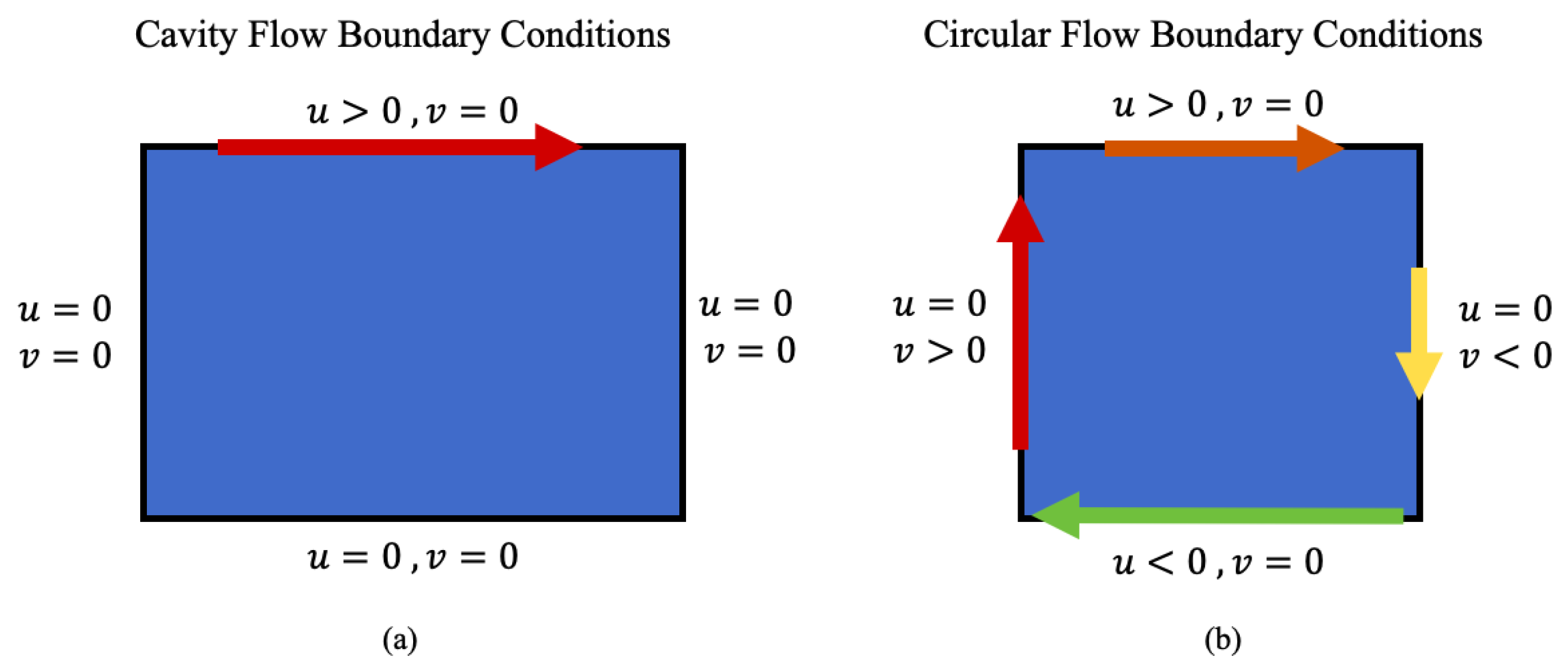
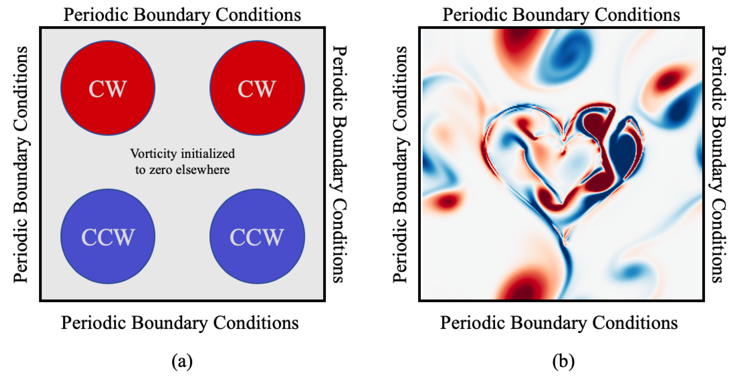
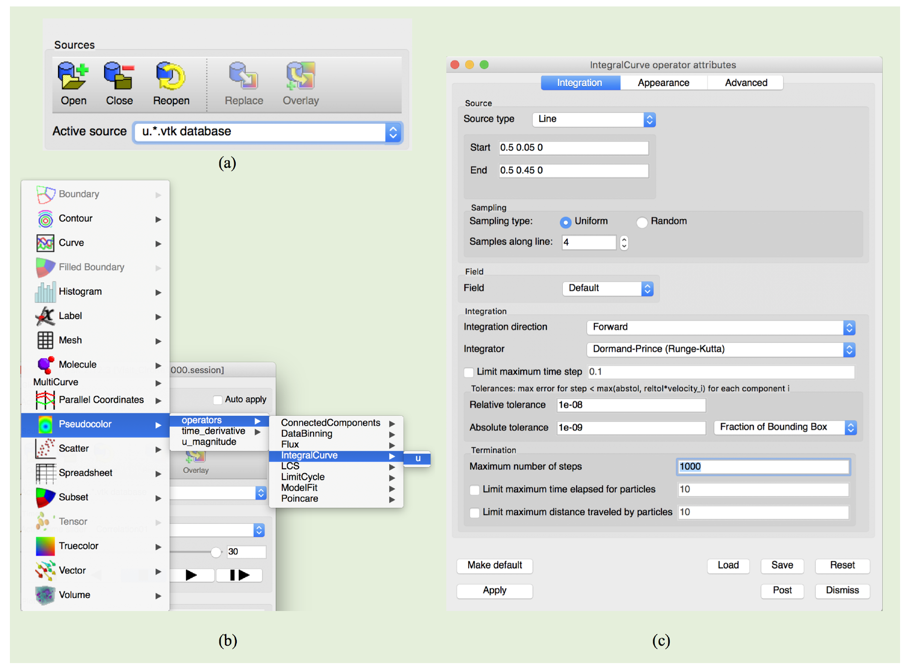
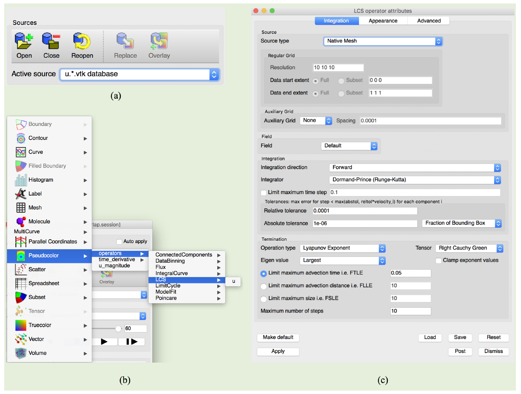
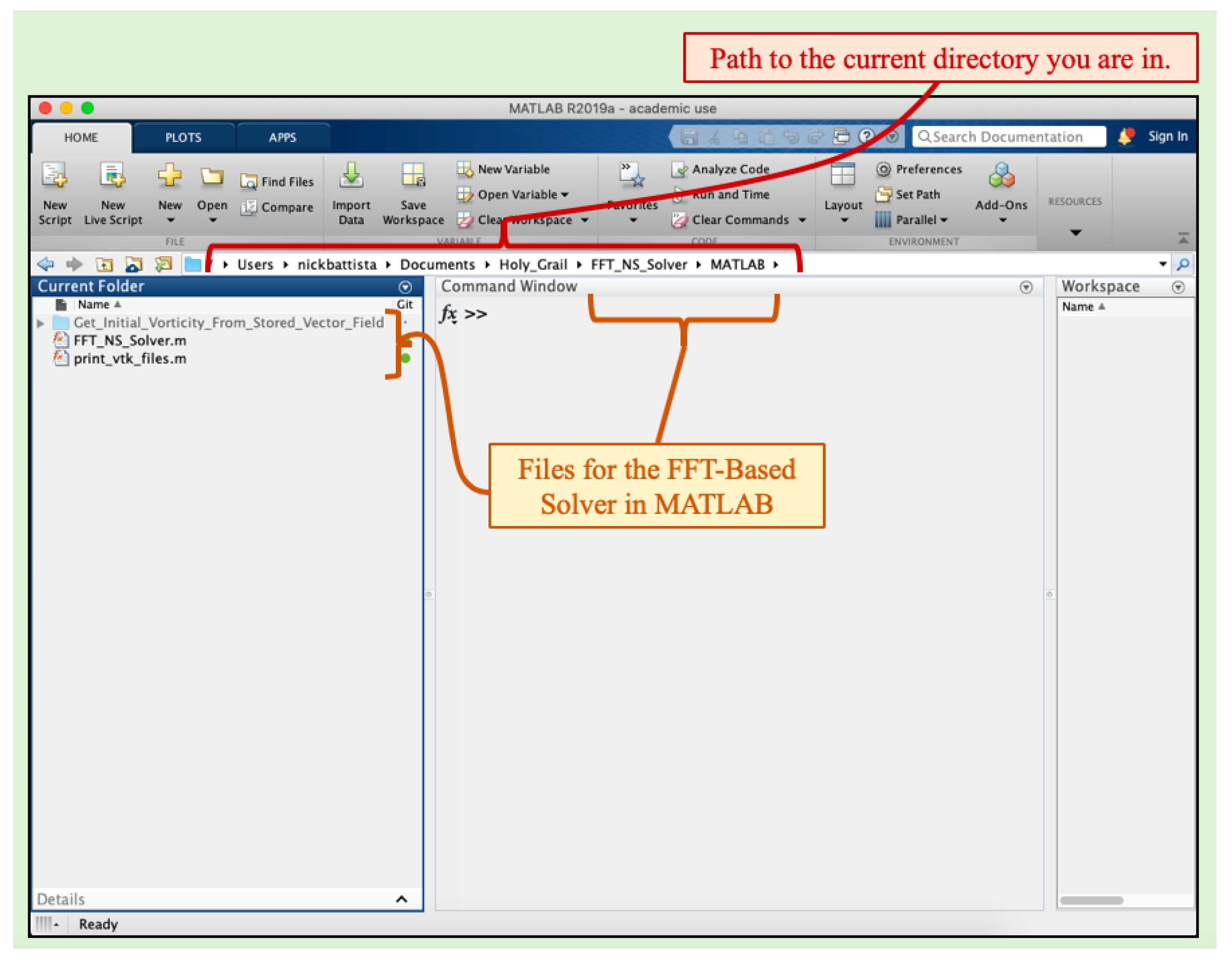
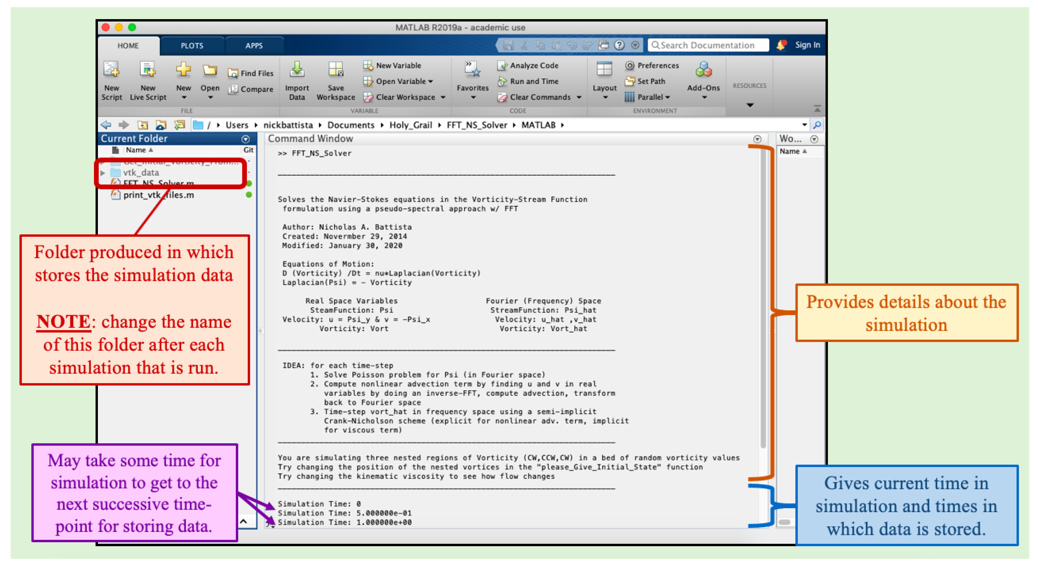
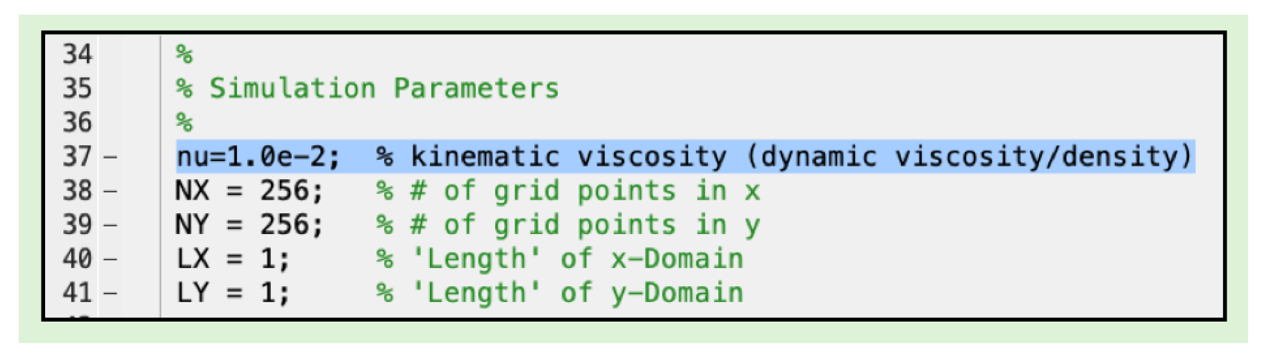
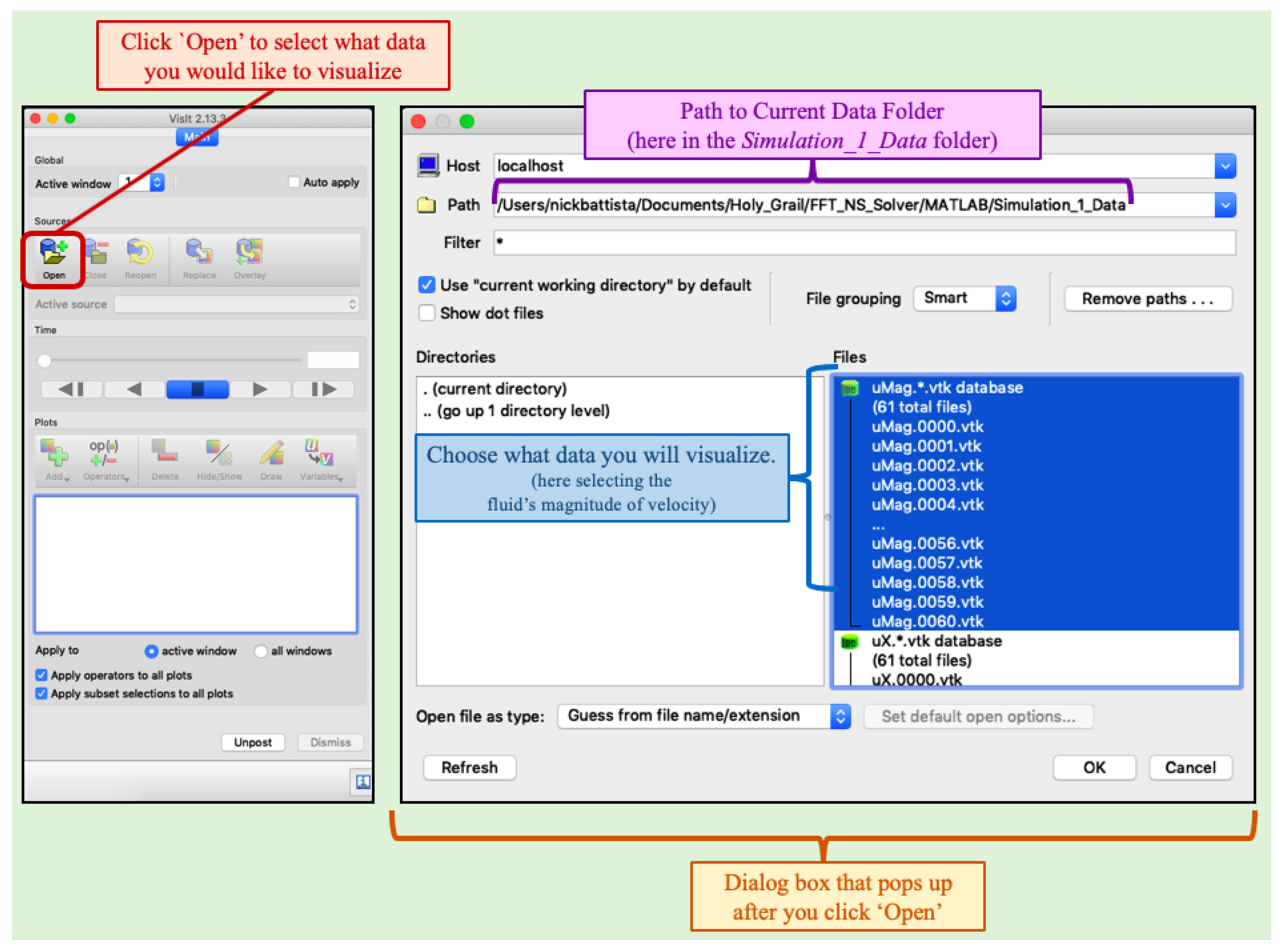
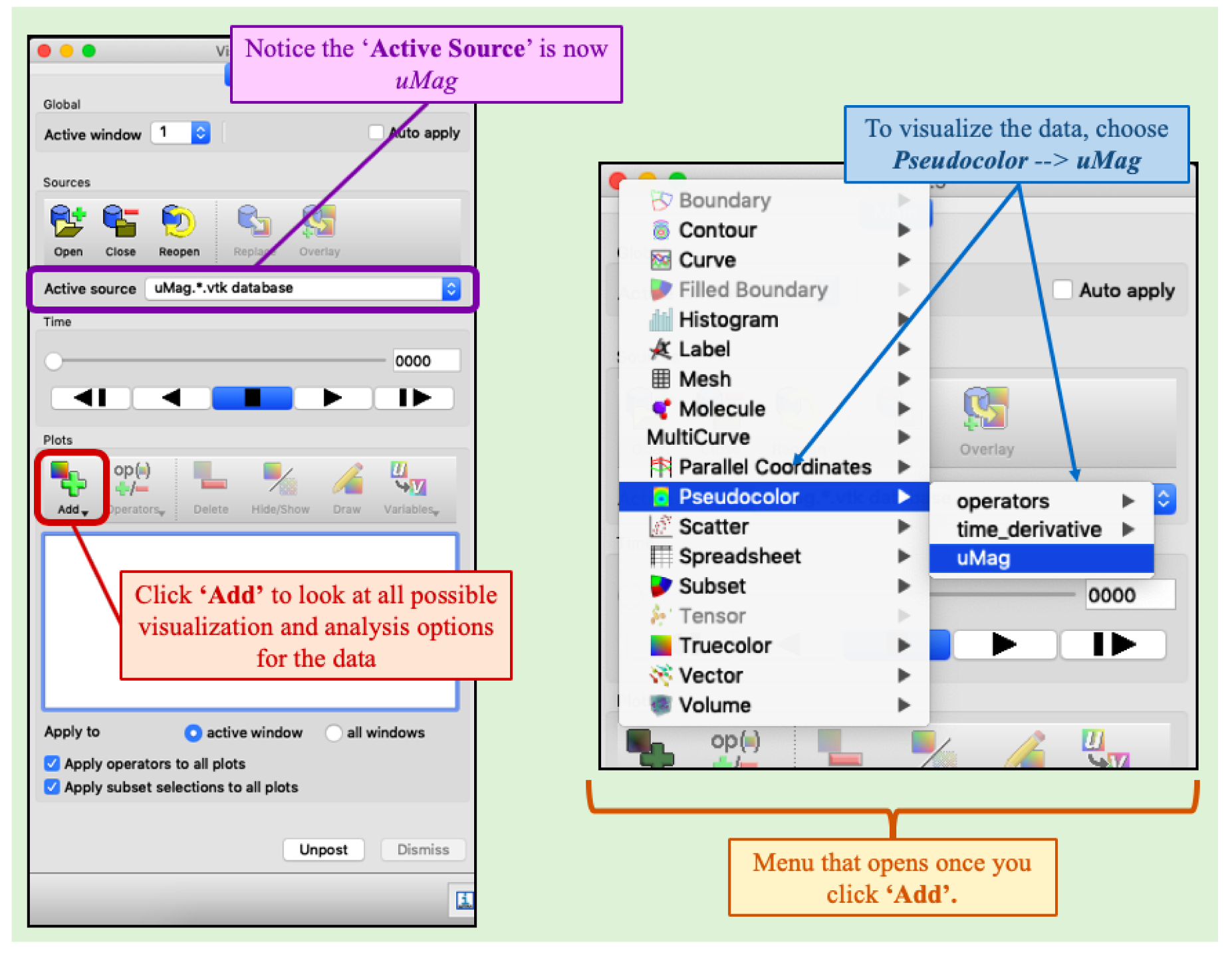
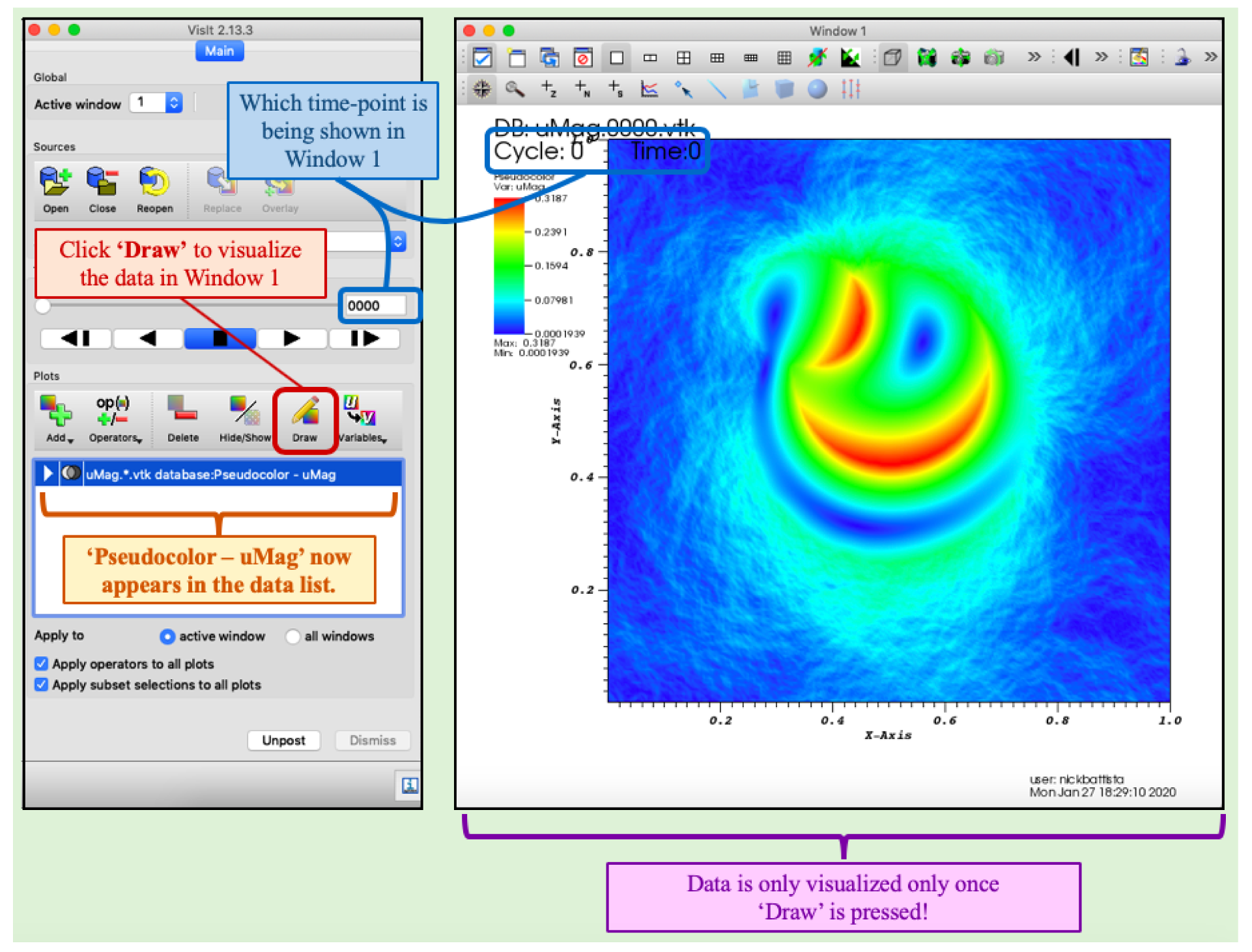
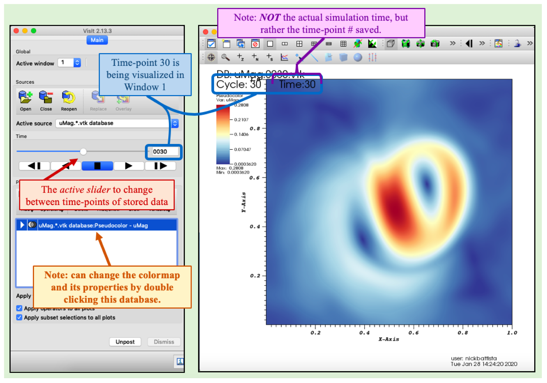
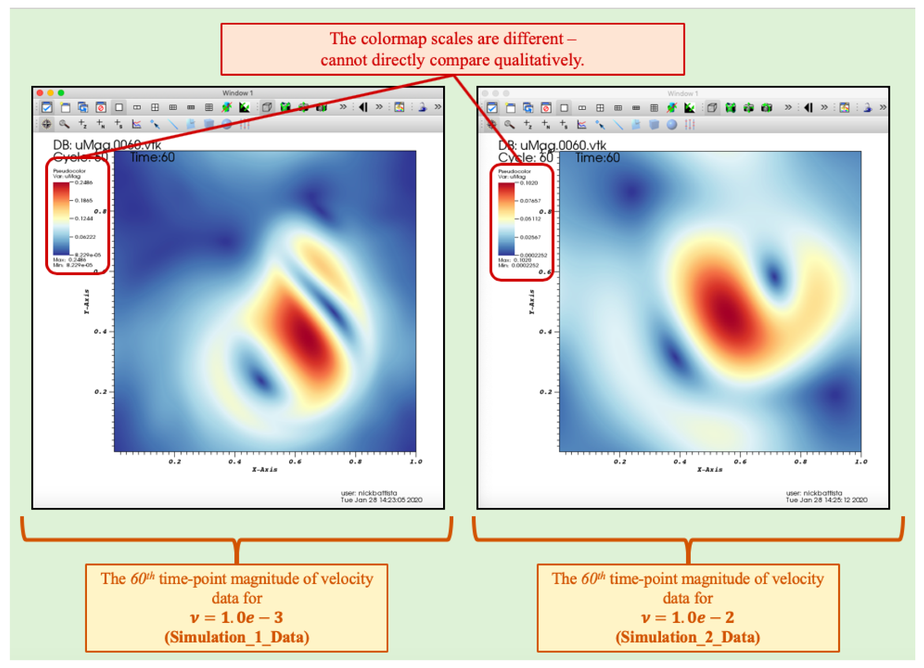
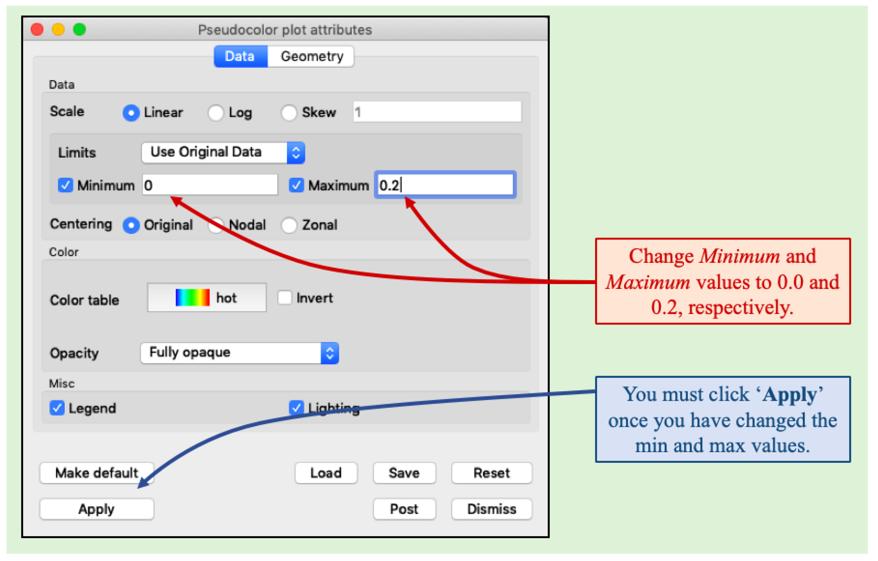
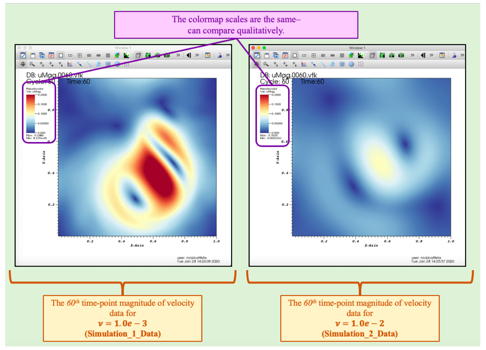
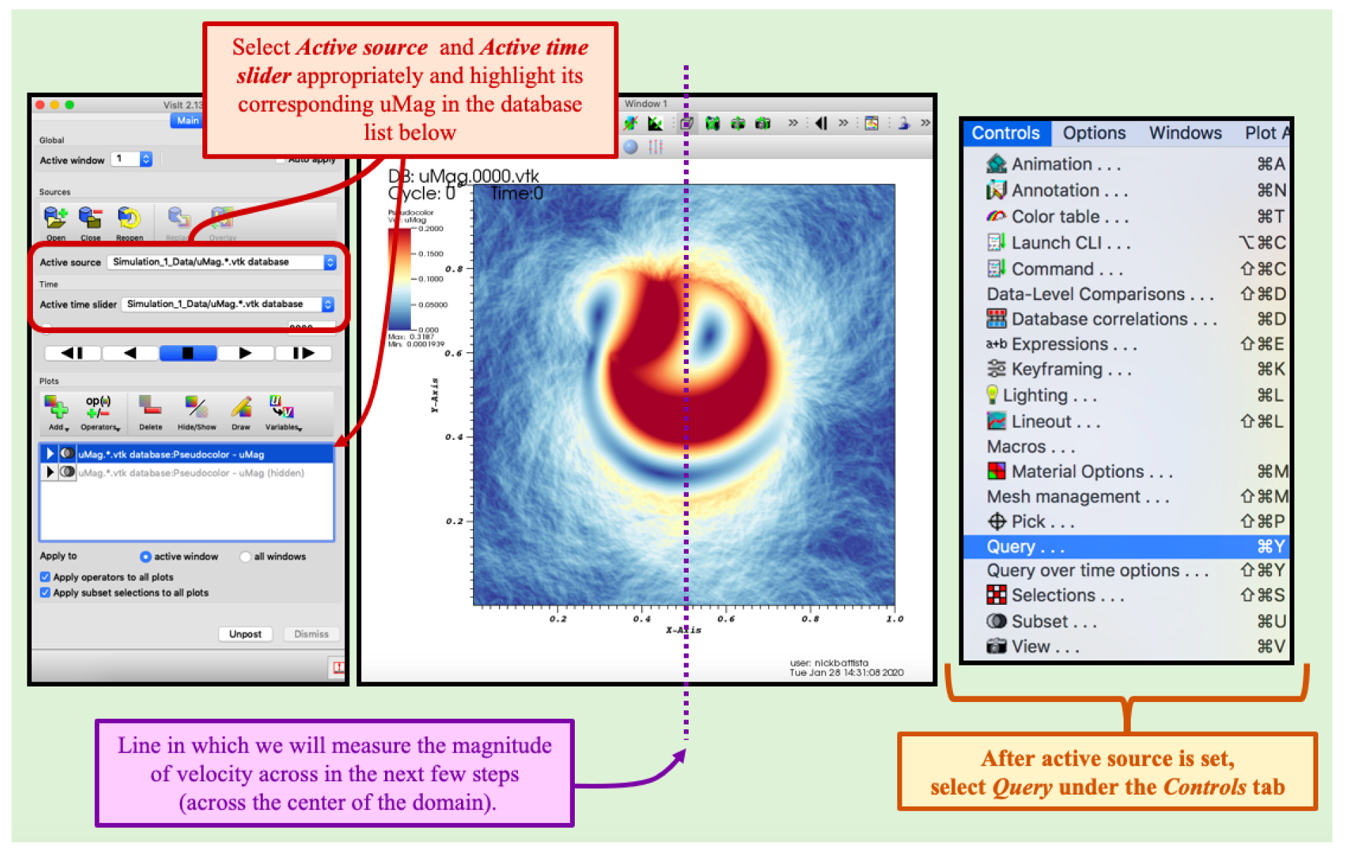
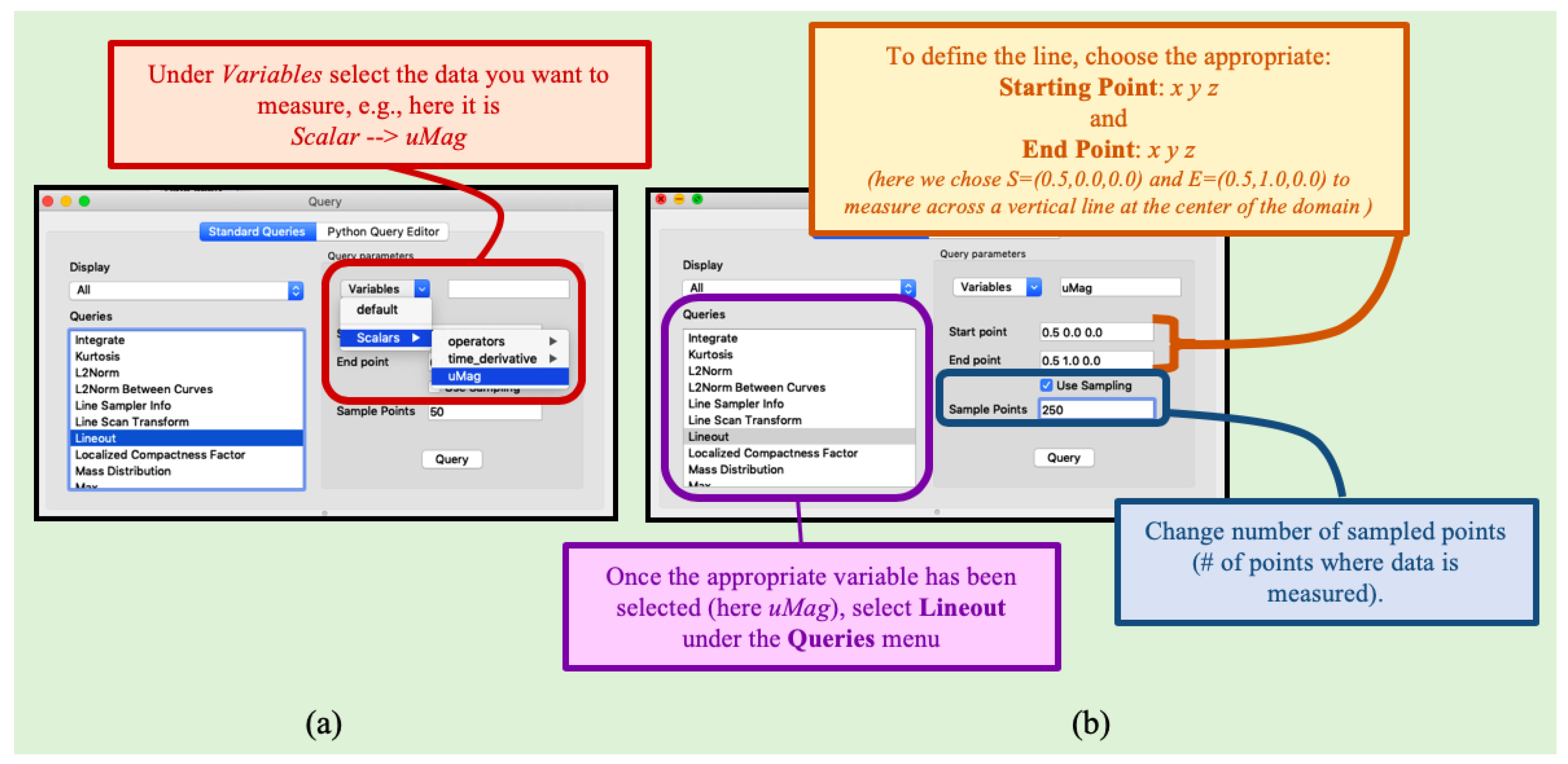
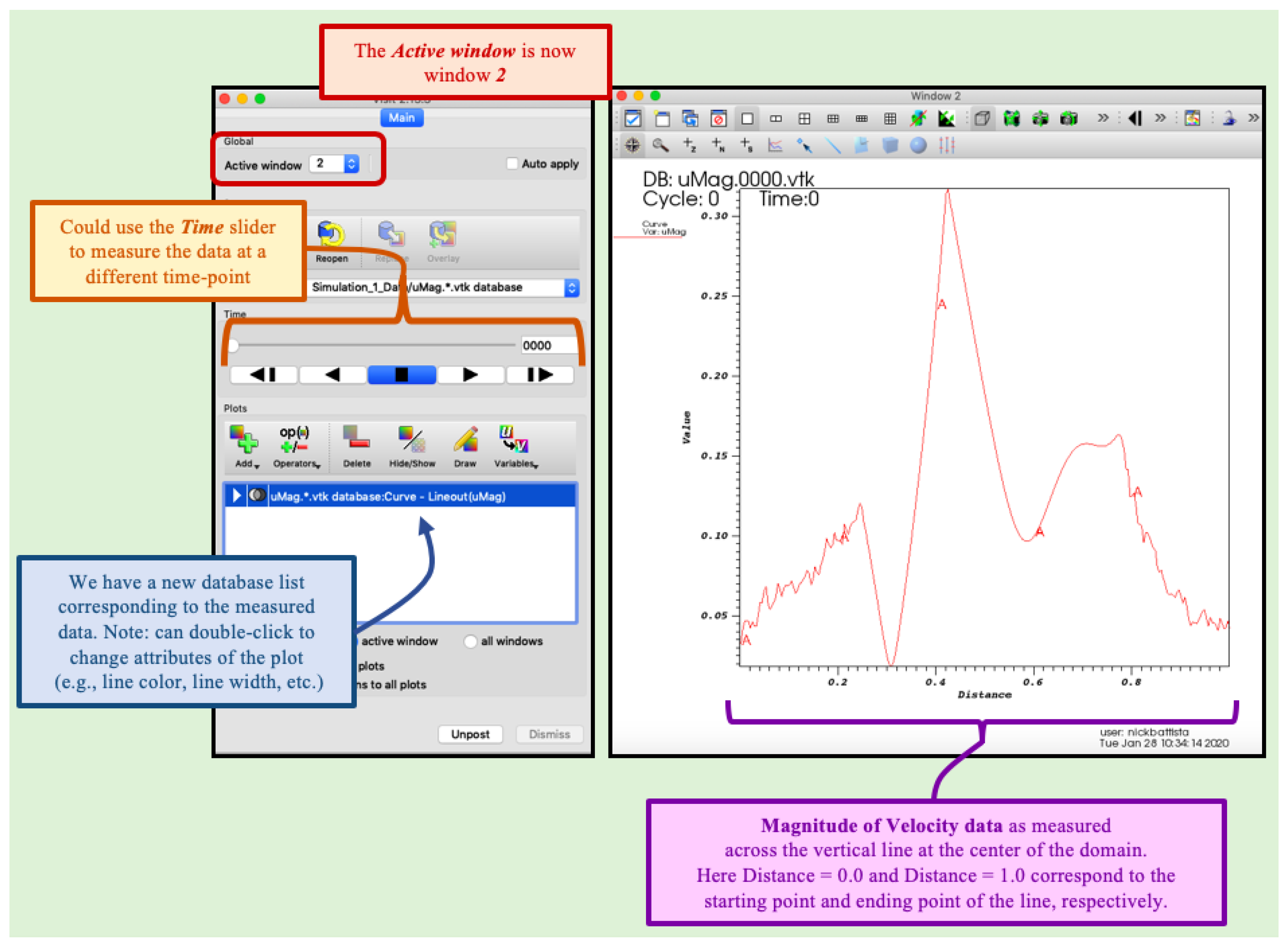
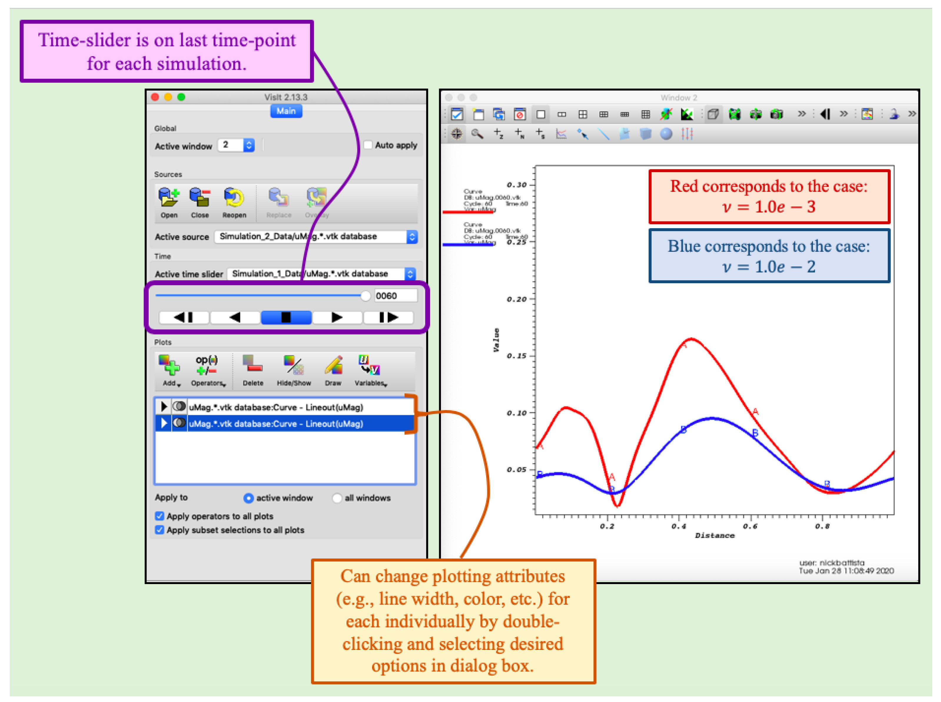
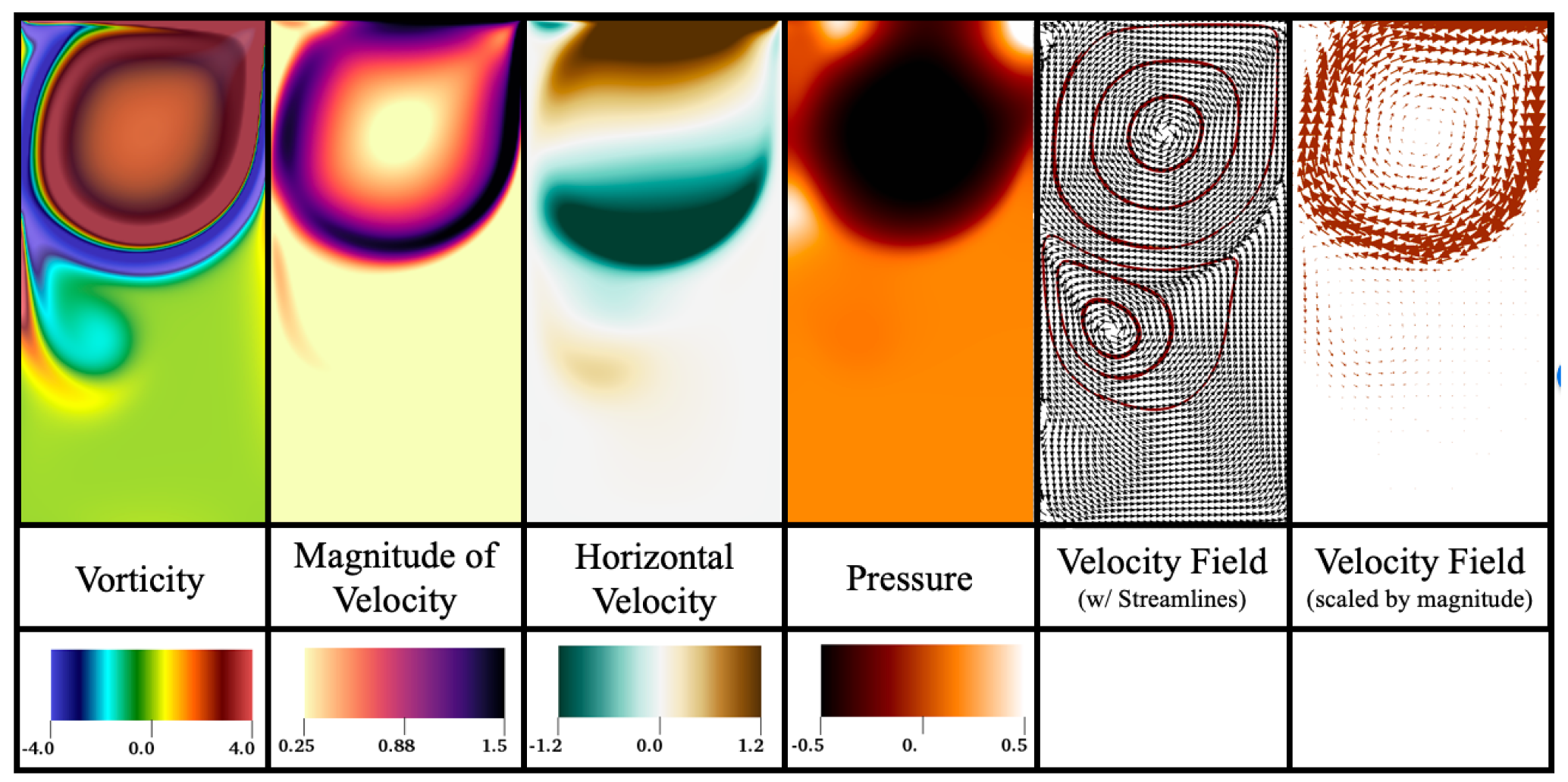
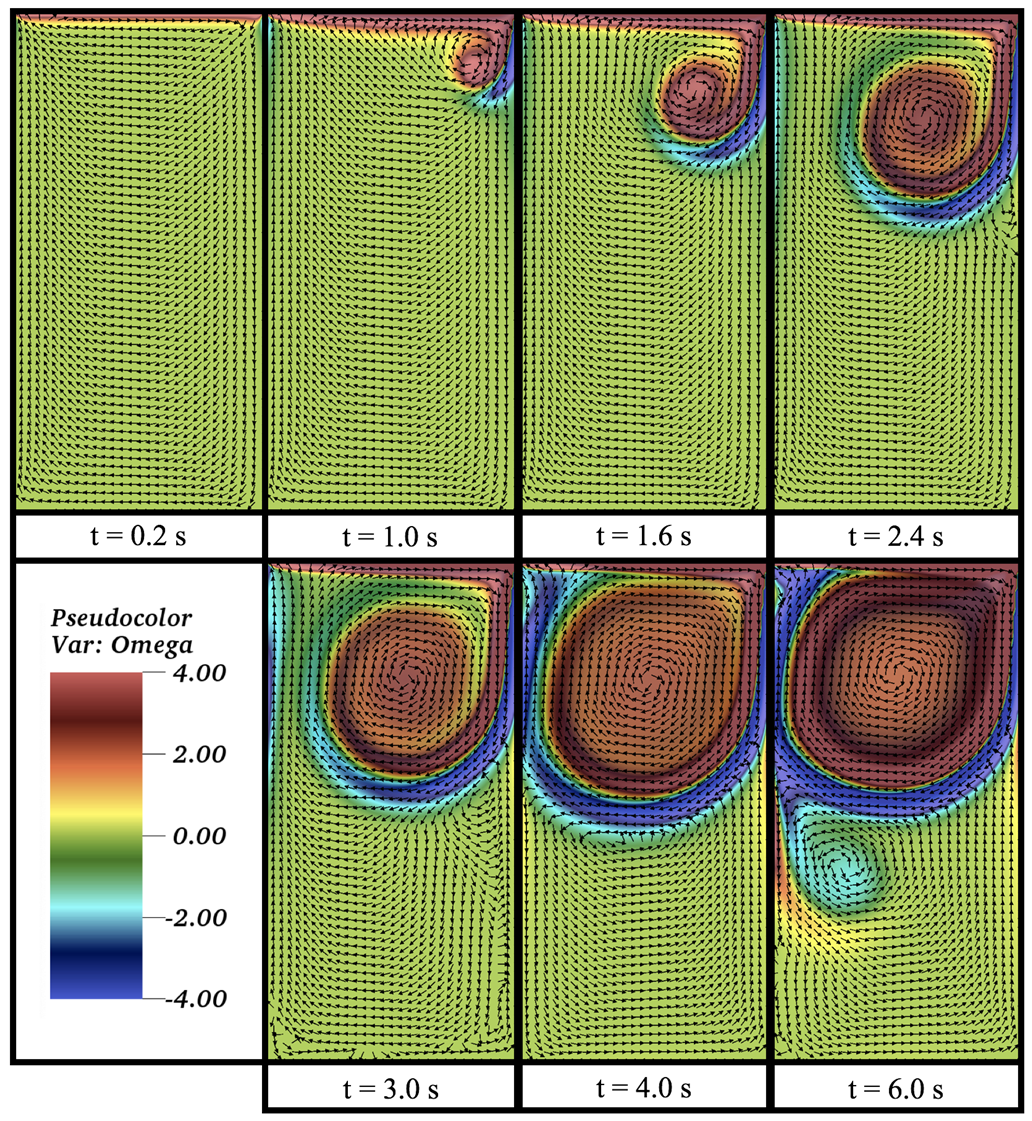
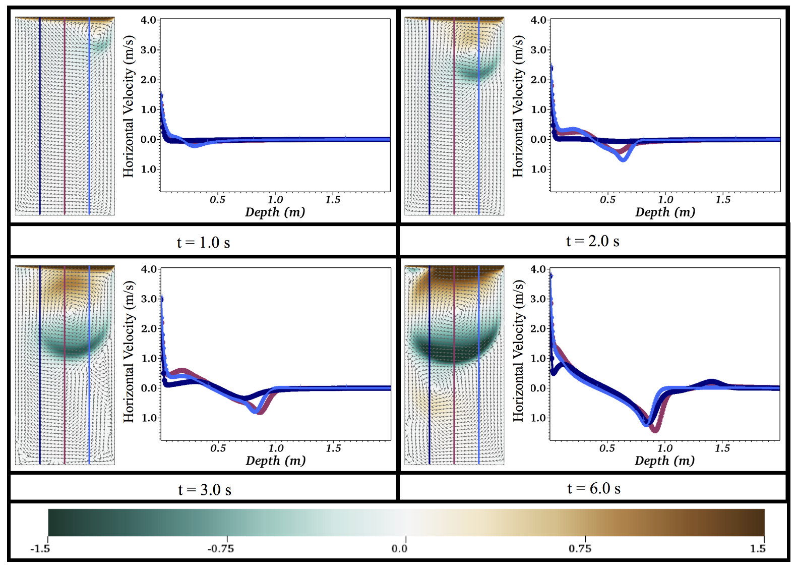
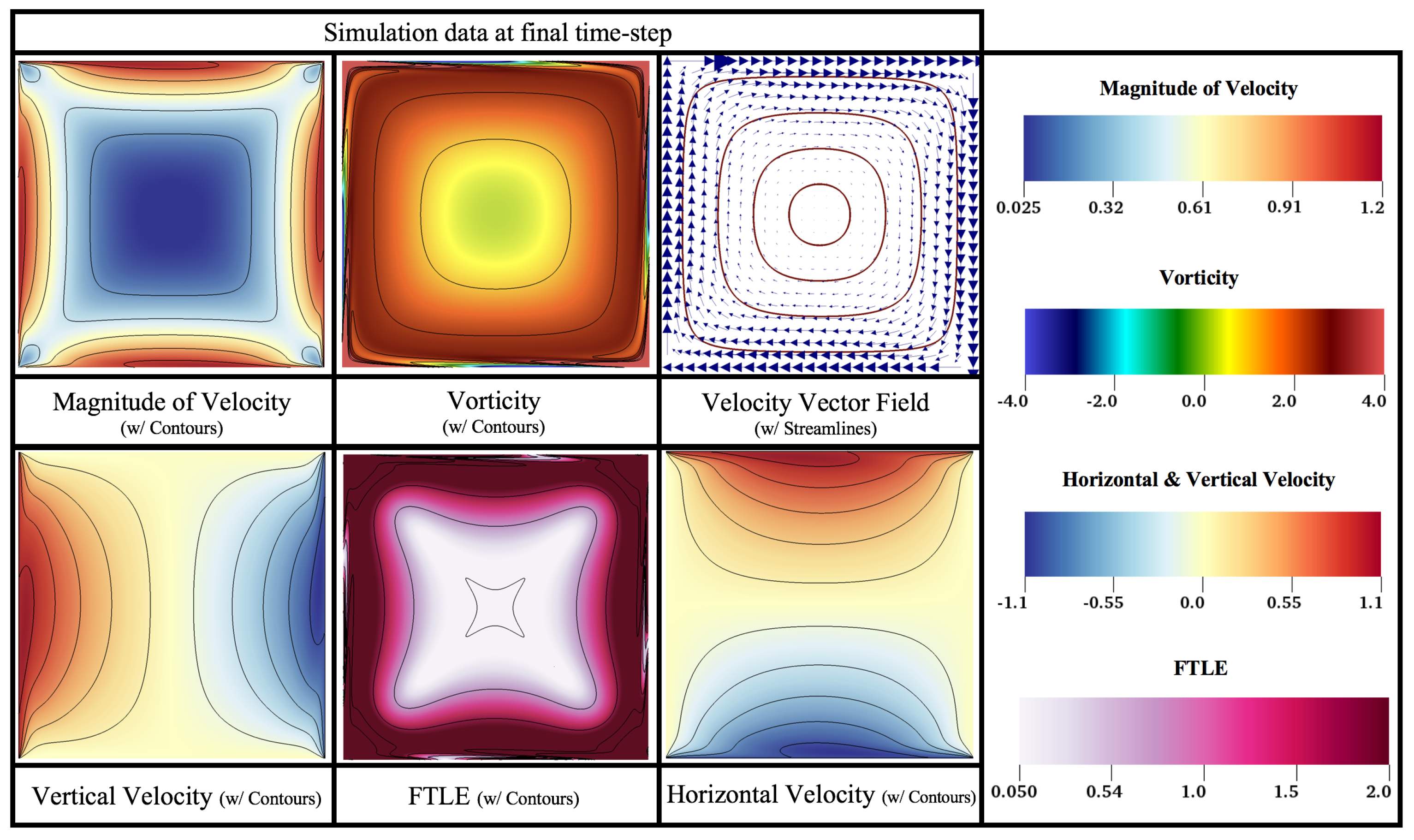
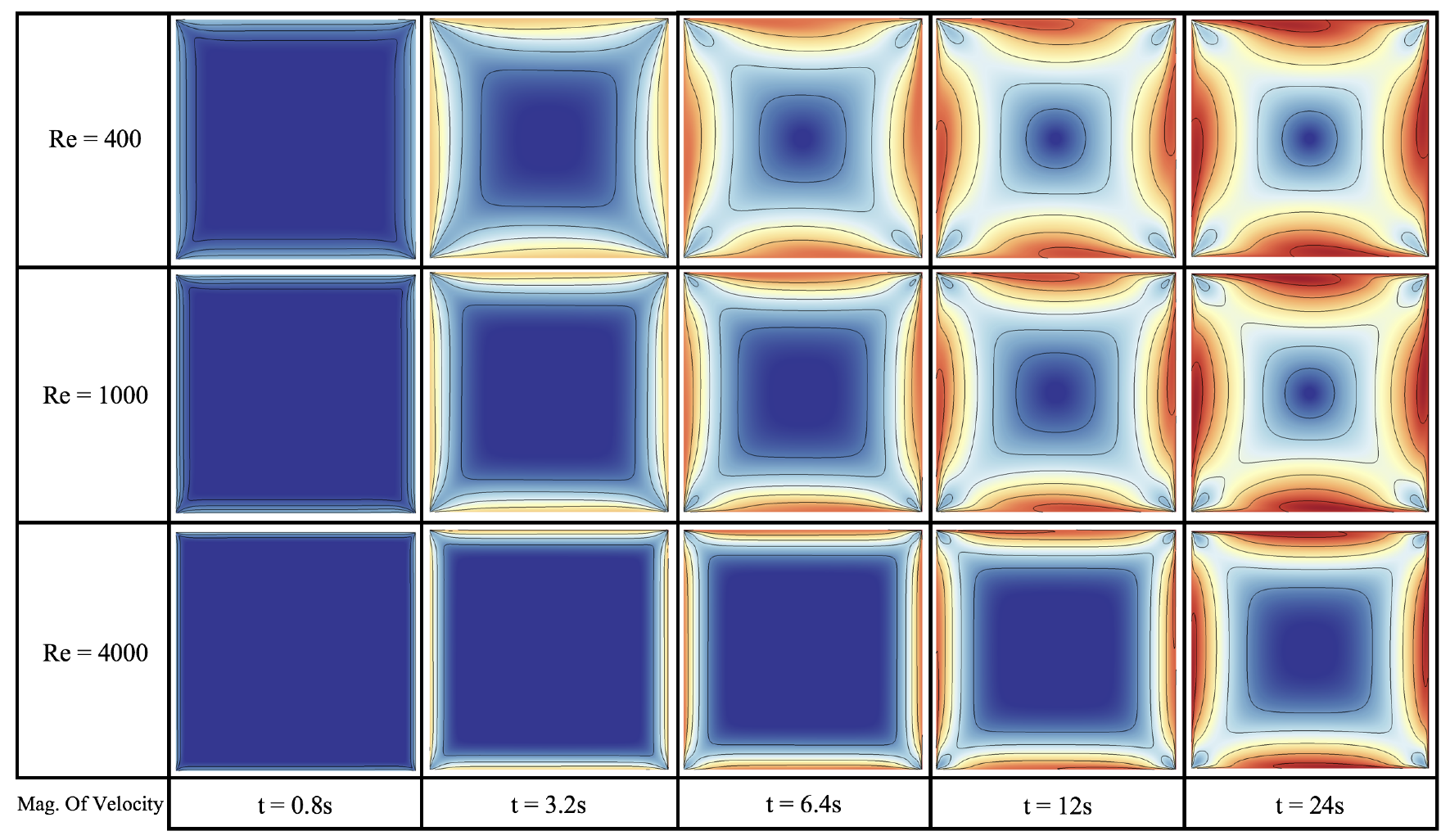
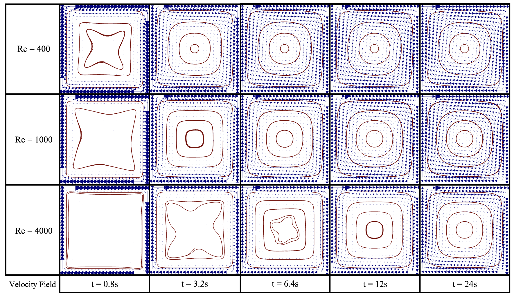
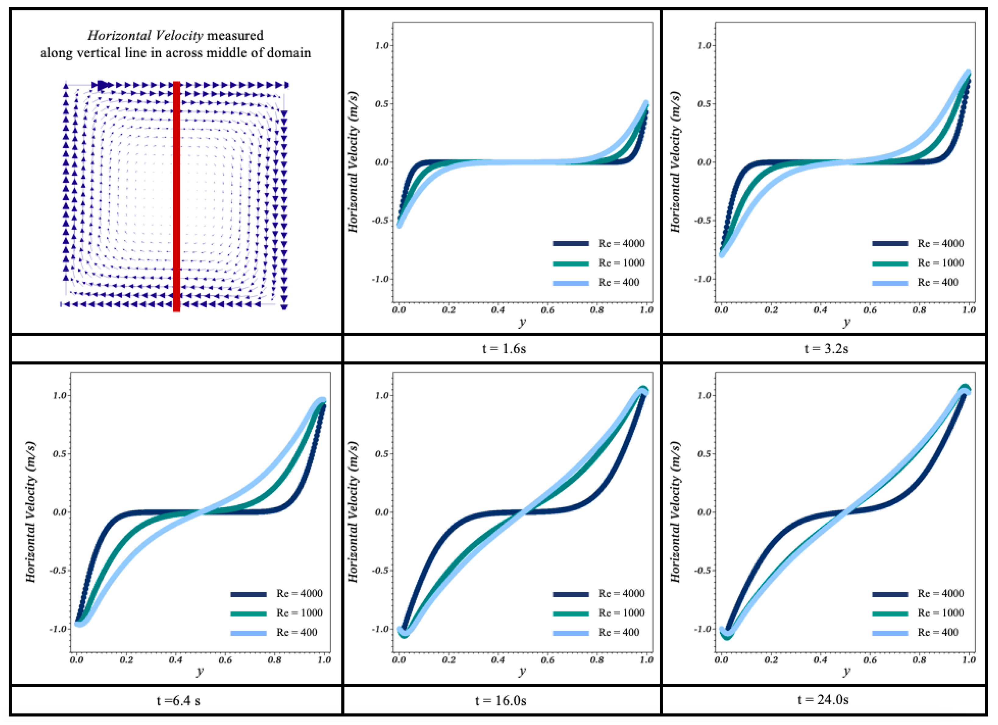
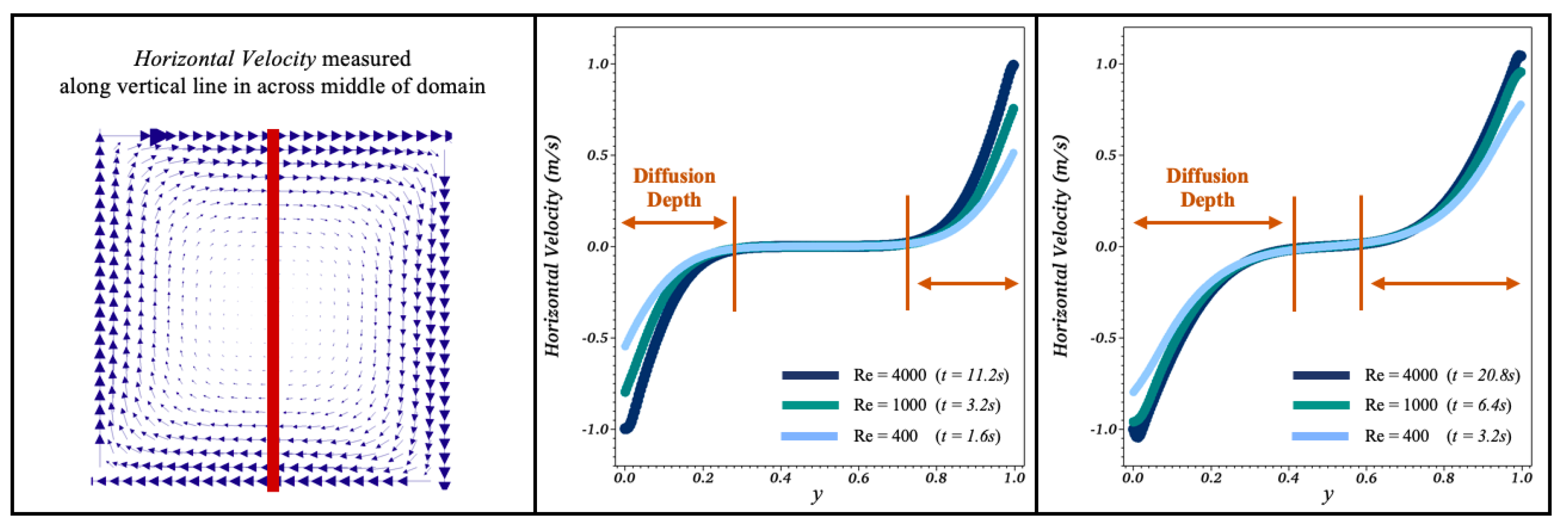
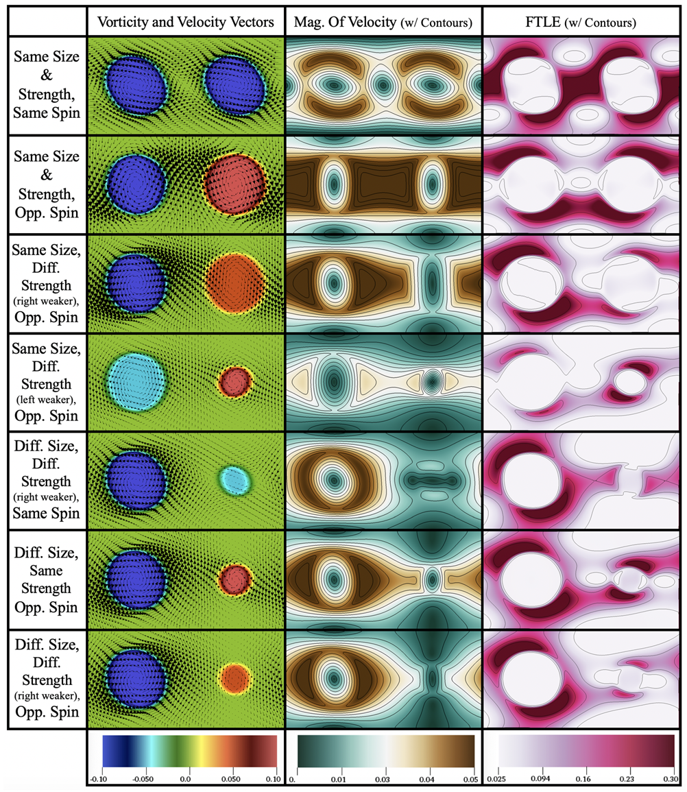
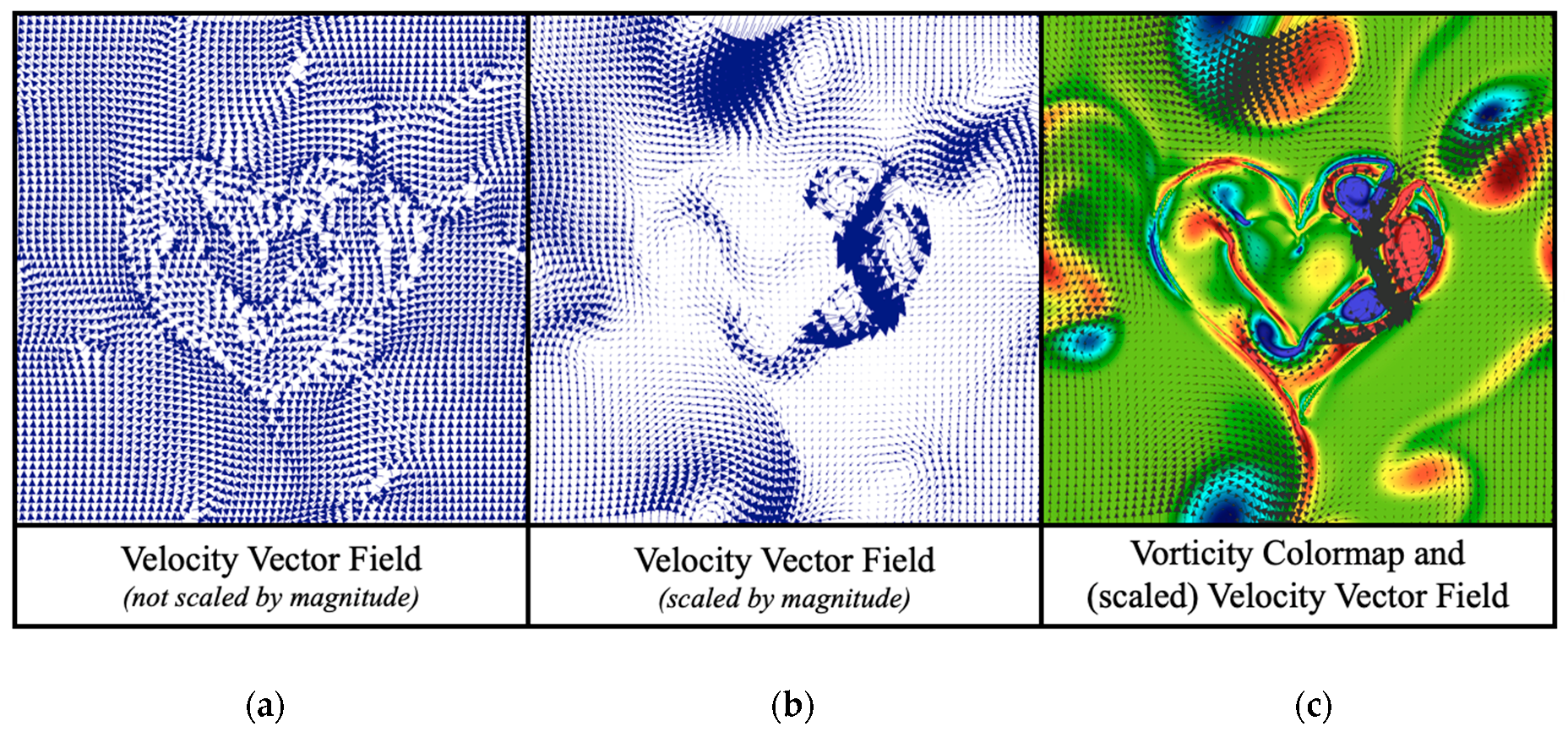
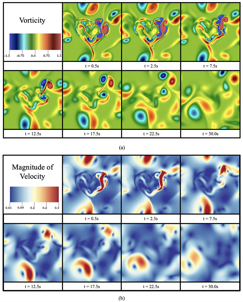
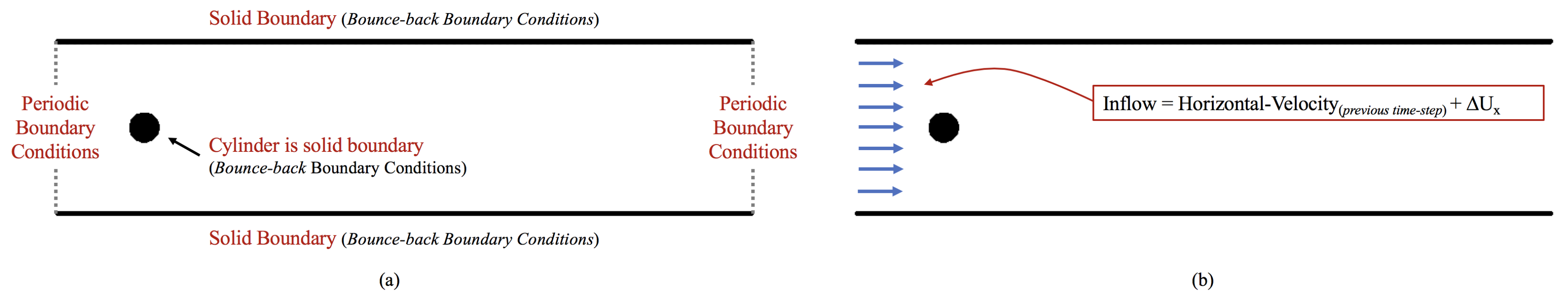
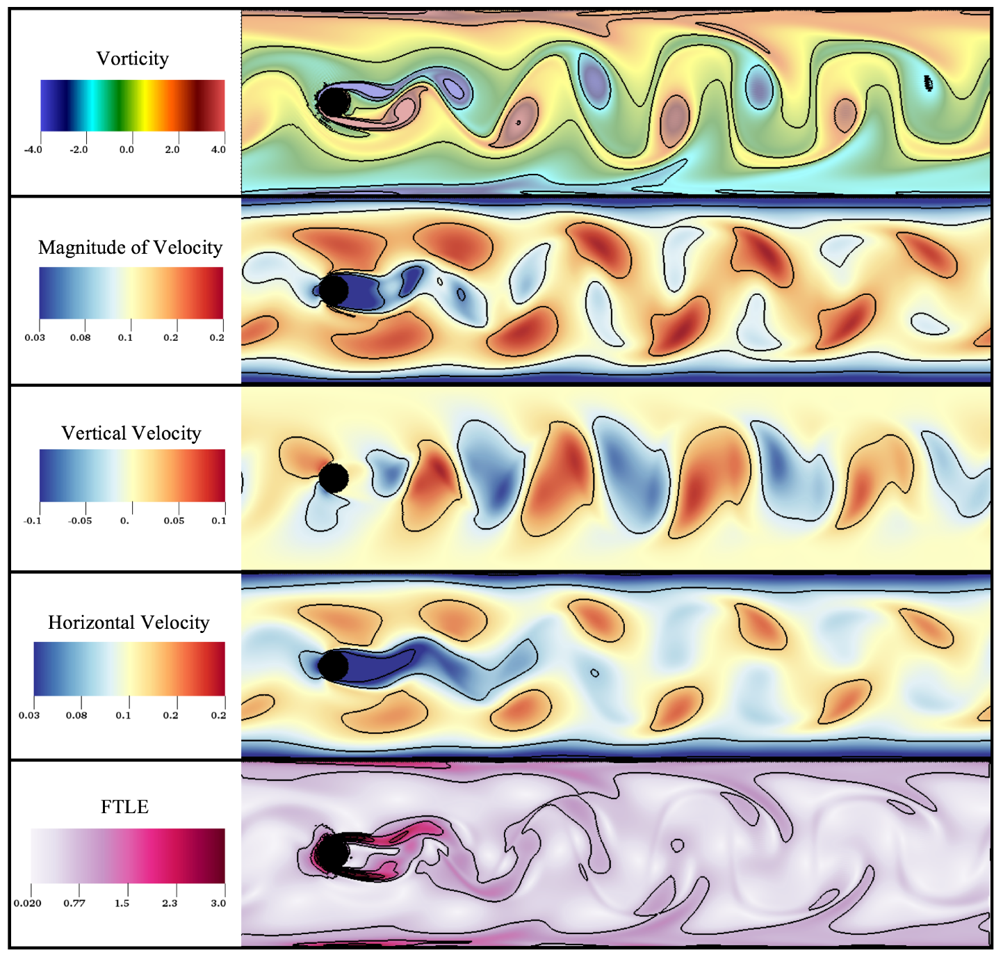
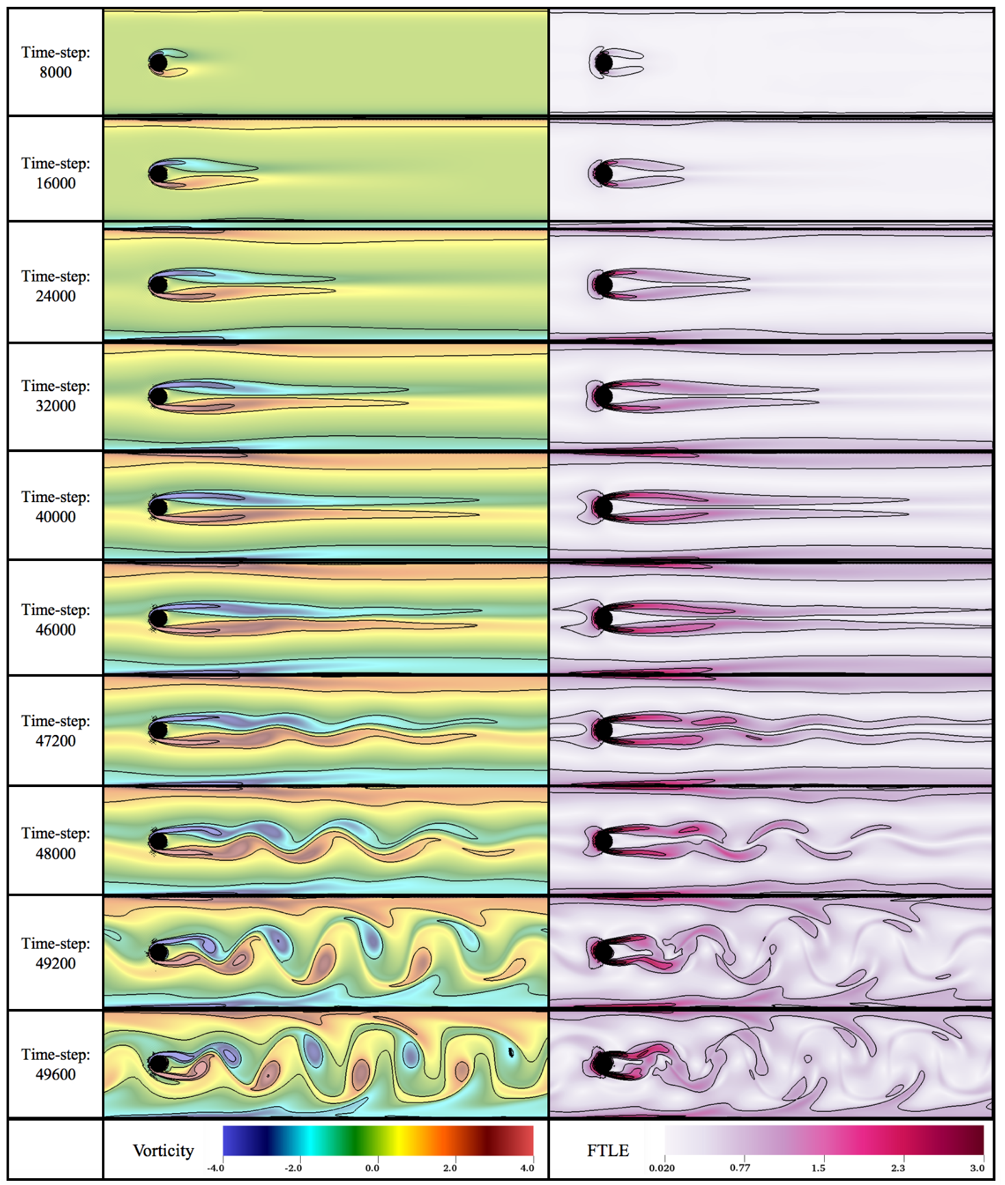
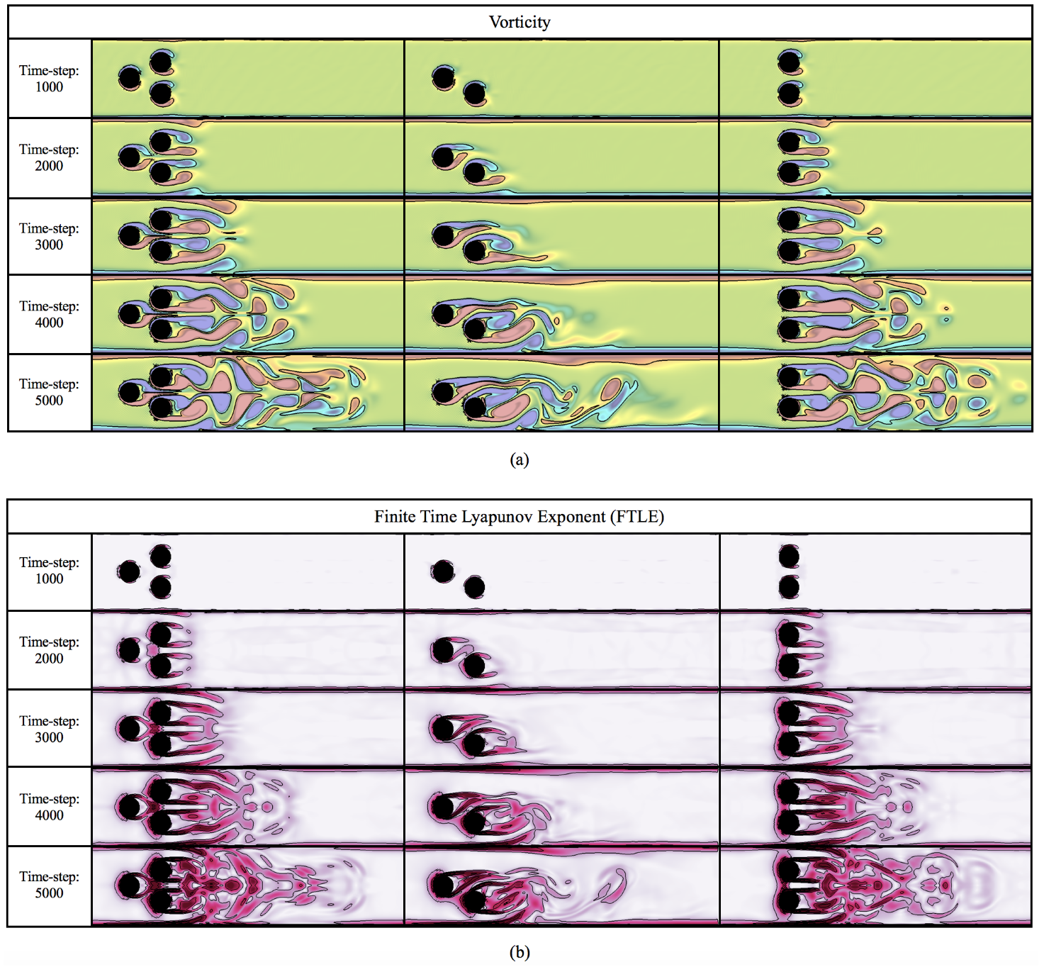
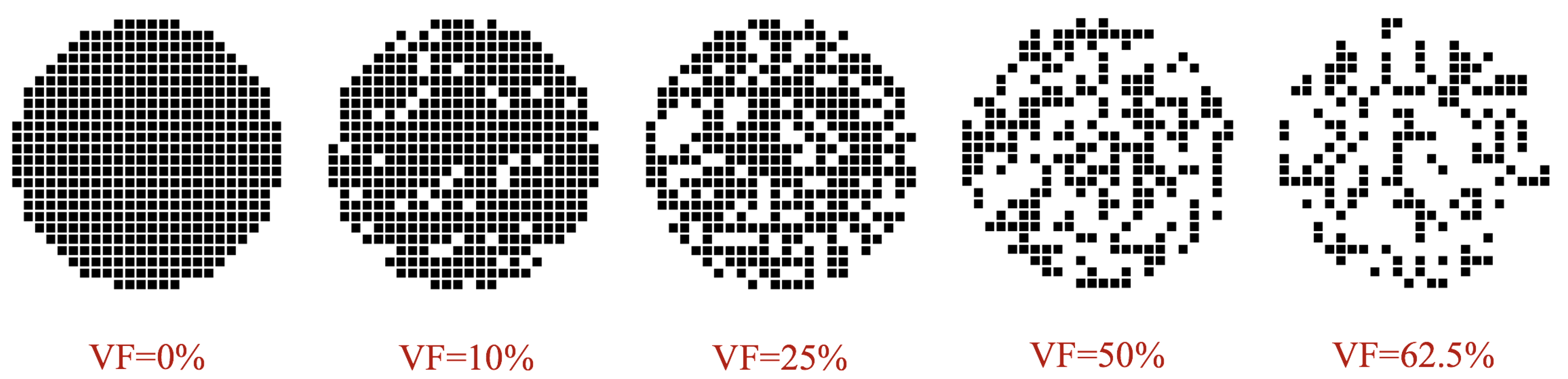
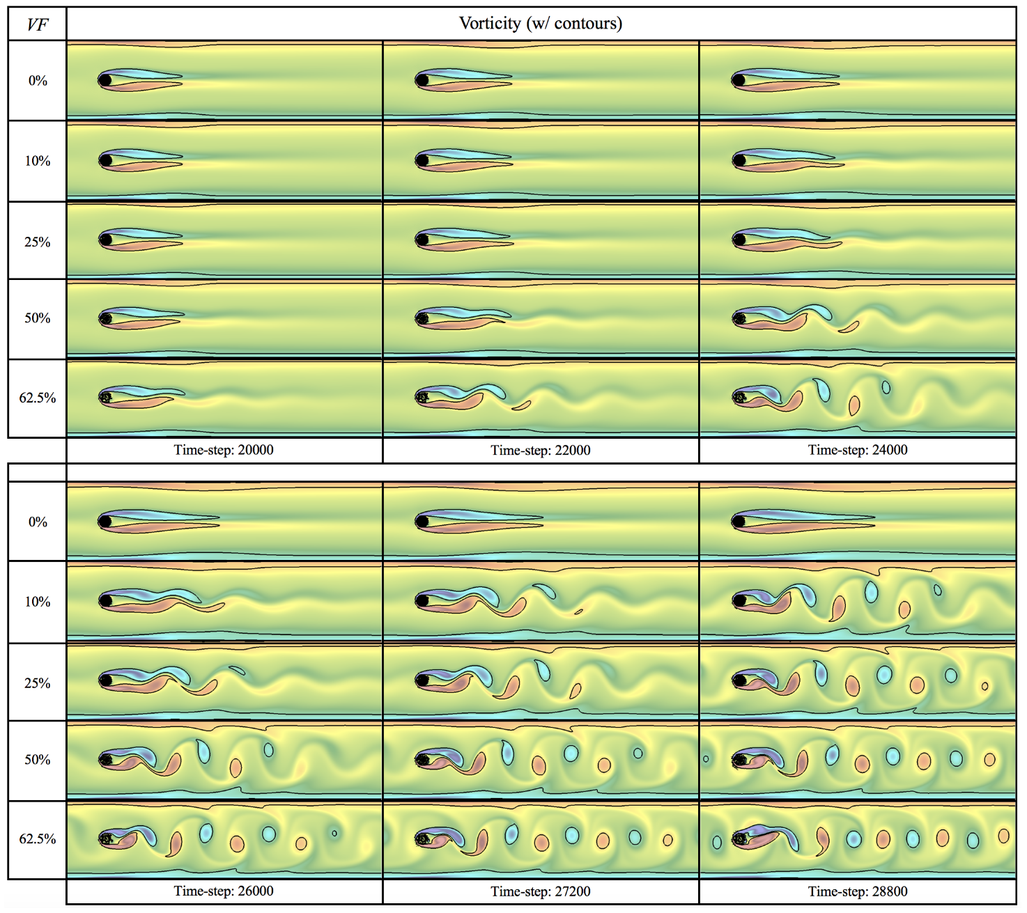
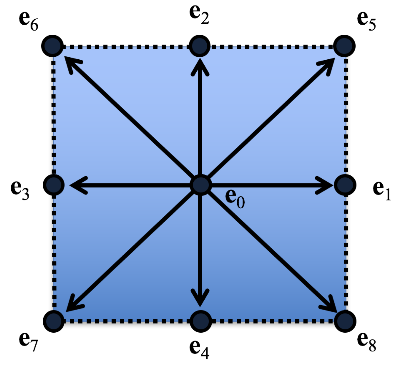
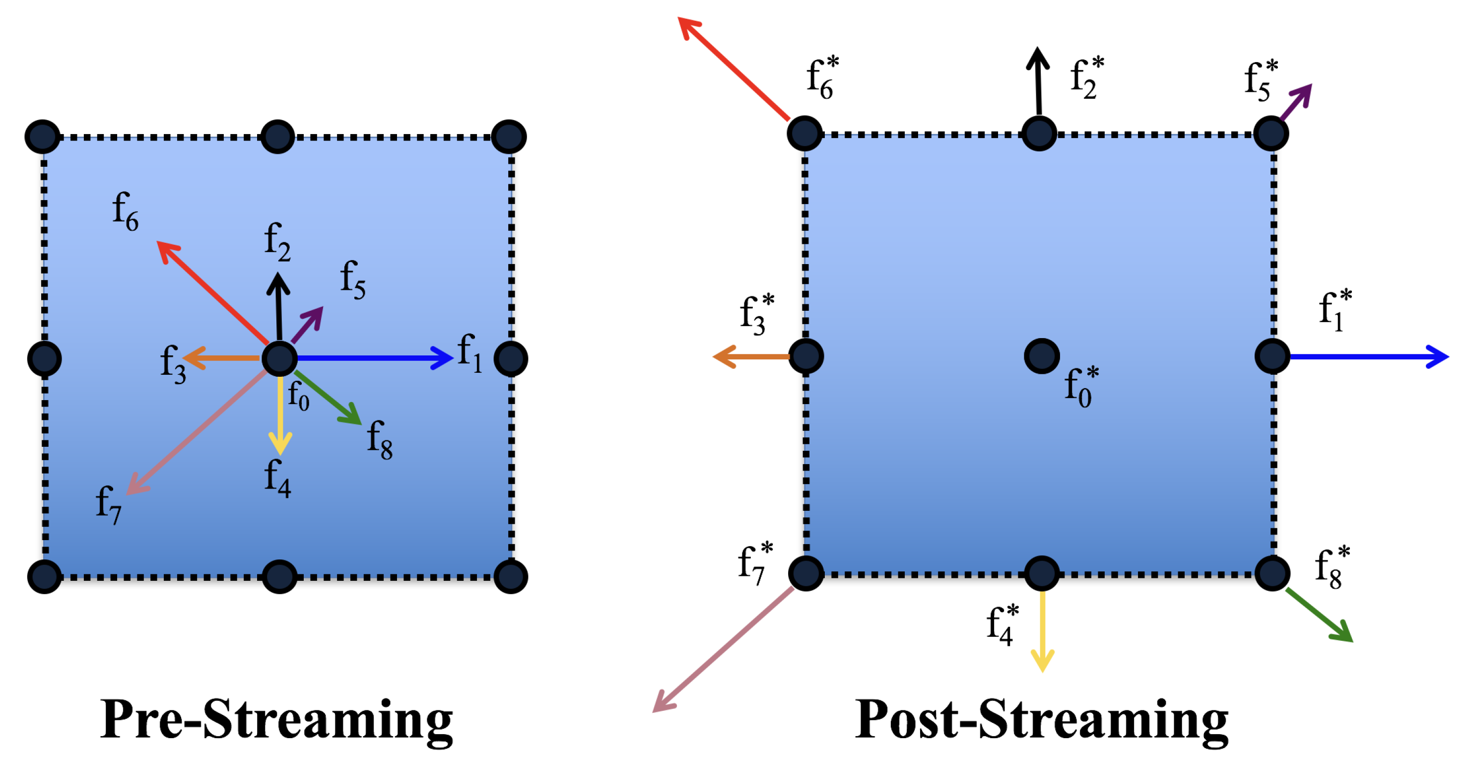
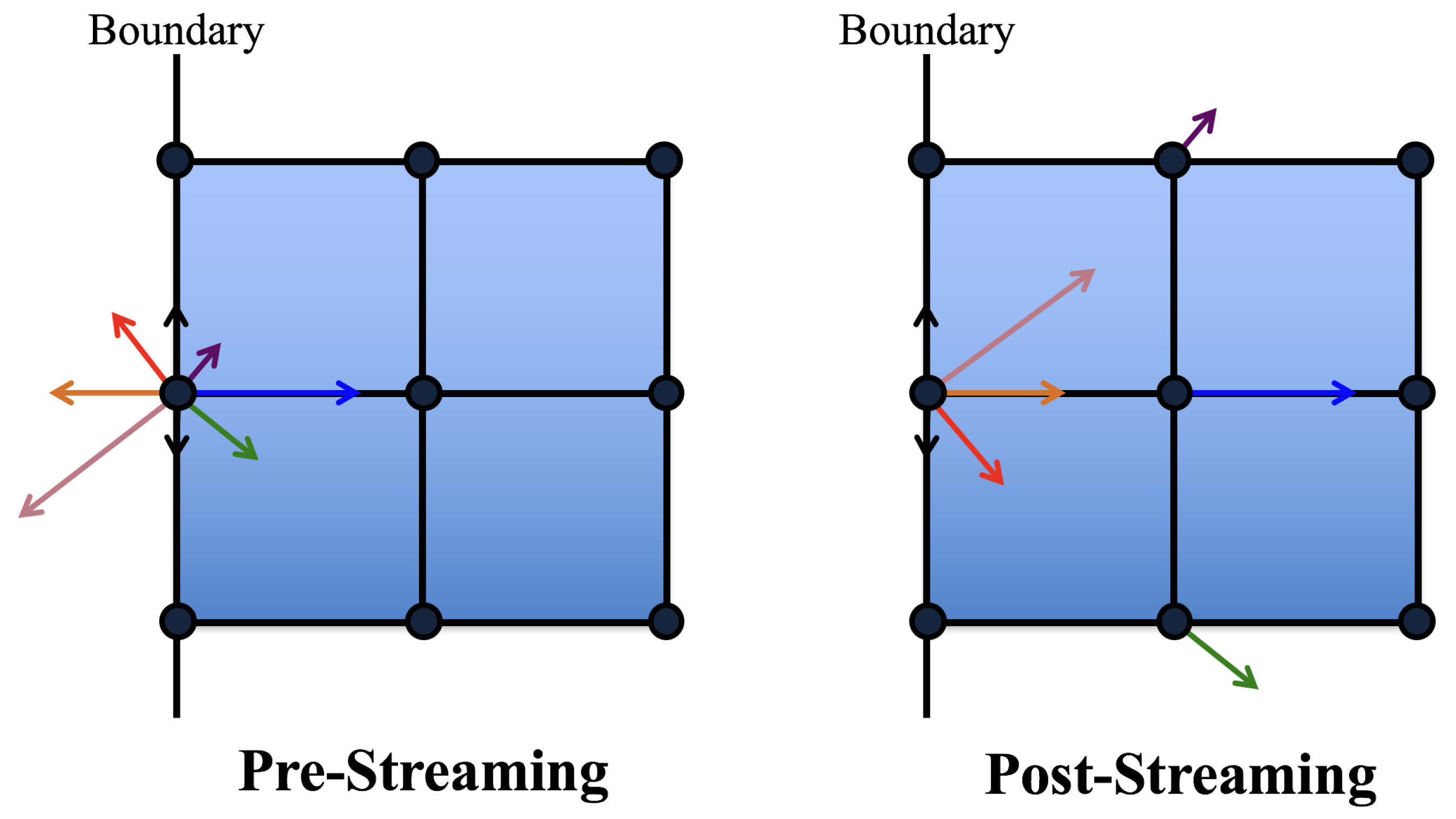
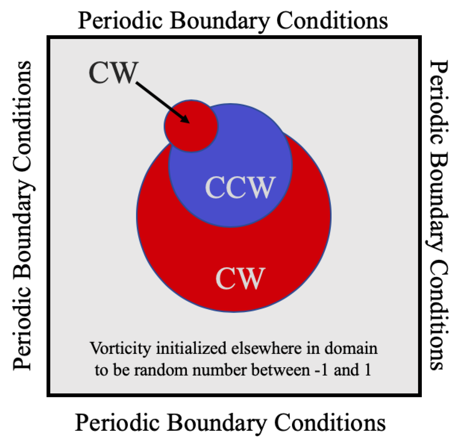
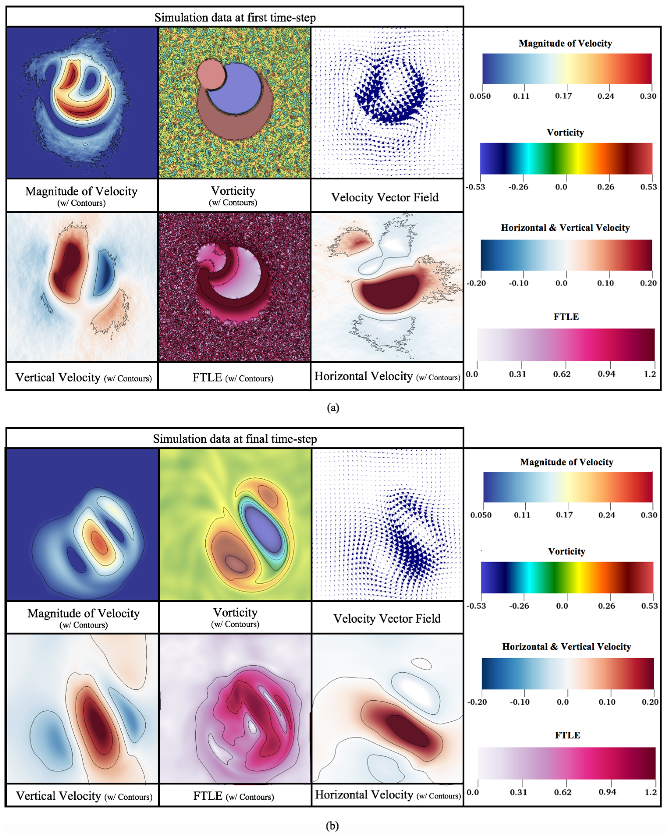
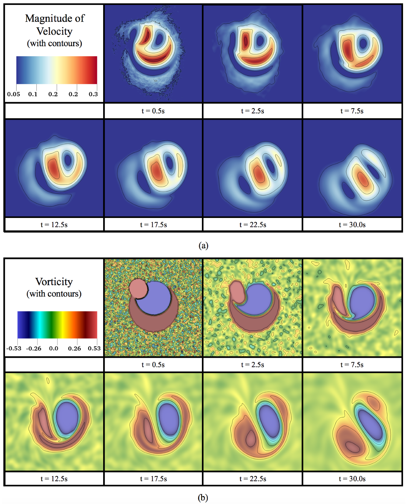
Table A1.
Numerical parameters for case with ‘overlapping’ vorticity regions
| Parameter | Variable | Units | Value |
|---|---|---|---|
| Domain Size | m | ||
| Spatial Grid Resolution | |||
| Spatial Grid Size | m | ||
| Time Step Size | s | ||
| Total Simulation Time | T | s | 30 |
| Fluid Kinematic Viscosity | m/s |
Figure A5 provides the simulation data at the beginning of the simulation (a) and at the last time-step (b). It presents colormaps (and corresponding contours) for vorticity, magnitude of velocity, horizontal velocity, vertical velocity, and the finite-time Lyapunov exponent (FTLE). It also gives a snapshot of the velocity vector field. The last snapshot of the simulation was from .
From Figure A5, it is evident that the random vorticity values at the start of the simulation eventually interact and dissipate in the flow, as observed in the vorticity panel. Initially there appears to be a lot of noise in the background vorticity (it was initialized to be random between [−1,1]) and by the end it appears virtually averaged out. Moreover, due to the background vorticity noise at the beginning, there are a lot of tiny patches of oppositely moving fluid. This leads to an initial background of high FTLE values, which suggests there is significant fluid mixing occurring. Similarly to vorticity, by the end, the background has significantly less mixing (e.g., smaller FTLE values) overall in areas away from the interacting vortical structures, which started off as overlapping vorticity regions. The area of high mixing in the FTLE panel at the last time-step is in a region where there is a lot of oppositely moving fluid, both horizontally as well as vertically.
Figure A5.
Simulation data from the case of overlapping vorticity regions during (a) the first time-step and (b) the final time-step.
Figure A5.
Simulation data from the case of overlapping vorticity regions during (a) the first time-step and (b) the final time-step.

Figure A6 provides snapshots over the simulation to illustrate how the magnitude of velocity and vorticity evolved over time. Figure A6a shows that the overlapping regions of vorticity induce the highest flows overall, as quantified by magnitude of velocity. That is, although the background was initialized to random values between [−1,1], which may include values that are higher than initial vorticity of the overlapping regions ( and for largest to smallest, respectively), it did not significantly contribute to bulk flow within the domain. Moreover, as suggested earlier, the initial random vorticity configuration quickly dissipates itself out, see Figure A6b.
Figure A6.
The evolution of (a) the magnitude of velocity (with its contours) and (b) vorticity (with its contours) during the course of the simulation.
Figure A6.
The evolution of (a) the magnitude of velocity (with its contours) and (b) vorticity (with its contours) during the course of the simulation.

Students may elect to try the following:
- Recreate the above results with the parameters listed in Table A1 or for different or computational domains.
- Change the initial vorticity in each ‘overlapping’ region.
- Change the placement of where each vorticity region is.
- Modify the example to have more/fewer overlapping regions of vorticity.
- Try initializing a completely random background vorticity without any other vorticity structures.
References
- Fefferman, C.L. Existence and Smoothness of the Navier-Stokes Equation. In The Millenium Prize Problems; Clay Mathematics Institute: Cambridge, MA, USA, 2006; pp. 57–67. [Google Scholar]
- Chorin, A.J. The numerical solution of the Navier-Stokes equations for an incompressible fluid. Bull. Am. Math. Soc. 1967, 73, 928–931. [Google Scholar] [CrossRef] [Green Version]
- Chorin, A.J. Numerical Solution of the Navier-Stokes Equations. Math. Comp. 1968, 22, 745–762. [Google Scholar] [CrossRef]
- Temam, R. Une méthode d’approximation de la solution des équations de Navier-Stokes. Bull. Soc. Math. Franc. 1968, 96, 115–152. [Google Scholar] [CrossRef] [Green Version]
- Brown, D.L.; Cortez, R.; Minion, M.L. Accurate Projection Methods for the Incompressible Navier-Stokes Equations. J. Comp. Phys. 2001, 168, 464–499. [Google Scholar] [CrossRef] [Green Version]
- Griffith, B.E. An accurate and efficient method for the incompressible Navier-Stokes equations using the projection method as a preconditioner. J. Comput. Phys. 2009, 228, 7565–7595. [Google Scholar] [CrossRef]
- Costa, B. Spectral Methods for Partial Differential Equations. CUBO Math. J. 2004, 6, 1–32. [Google Scholar]
- Uecker, H. A short ad hoc introduction to spectral methods for parabolic PDE and the Navier-Stokes equations, 2009. In Proceedings of the Lecture given at International Summer School Modern Computational Science, Oldenburg, Germany, 16–28 August 2009. [Google Scholar]
- Suzuki, M. Fourier-Spectal Methods For Navier-Stokes Equations in 2D. 2014. Available online: http://www.math.mcgill.ca/gantumur/math595f14/NSMashbat.pdf (accessed on 29 June 2019).
- Hardy, J.; Pomeau, Y.; de Pazzis, O. Time evolution of a two-dimensional classical lattice system. Phys. Rev. Lett. 1973, 31, 276–279. [Google Scholar] [CrossRef]
- Chen, S.; Doolen, G.D. Lattice Boltzmann method for fluid flows. Annu. Rev. Fluid Mech. 1998, 30, 282–300. [Google Scholar] [CrossRef] [Green Version]
- Succi, S. The Lattice Boltzmann Equation for Fluid Dynamics and Beyond; Oxford University Press: Oxford, UK, 2001. [Google Scholar]
- Stern, F.; Xing, T.; Yarbrough, D.B.; Rothmayer, A.; Rajagopalan, G.; Prakashotta, S.; Caughey, D.; Bhaskaran, R.; Smith, S.; Hutchings, B.; et al. Hands-On CFD Educational Interface for Engineering Courses and Laboratories. J. Eng. Edu. 2006, 95, 63–83. [Google Scholar] [CrossRef]
- Cummings, R.; Morton, S. Computational Aerodynamics Goes to School: A Course in CFD for Undergraduate Students. In Proceedings of the 43rd AIAA Aerospace Sciences Meeting and Exhibit, Reno, NV, USA, 10–13 January 2005; AIAA: Reston, VA, USA, 2005. [Google Scholar] [CrossRef] [Green Version]
- Ormiston, S.J. Incorporating CFD into the undergraduate Mechanical Engineering Programme at the University of Manitoba. In Proceedings of the Ninth Annual Conference of the CFD Society of Canada: CFD2001, Waterloo, ON, Canada, 27–29 May 2001; Schneider, G., Ed.; CFD Society of Canada: Waterloo, ON, Canada, 2001; pp. 333–337. [Google Scholar]
- Aung, K. Design and Implementation of an Undergraduate Computational Fluid Dynamics (Cfd) Course, 2003. In Proceedings of the 2003 American Society for Engineering Education Annual Conference, Nashville, TN, USA, 22–25 June 2003; Available online: https://peer.asee.org/design-and-implementation-of-an-undergraduate-computational-fluid-dynamics-cfd-course.pdf (accessed on 9 September 2019).
- Stern, F.; Xing, T.; Yarbrough, D.; Rothmayer, A.; Rajagopalan, G.; Otta, S.P.; Caughey, D.; Bhaskaran, R.; Smith, S.; Hutchings, B.; et al. Development of hands-on CFD educational interface for undergraduate engineering courses and laboratories. In Proceedings of the 2004 American Society for Engineering Education Annual Conference & Exposition, Salt Lake City, UT, USA, 20–23 June 2004; American Society for Engineering Education: Washington, DC, USA, 2004; pp. 1526–1555. [Google Scholar]
- Adair, D. Incorporation of Computational Fluid Dynamics into a Fluid Mechanics Curriculum. In Advances in Modeling of Fluid Dynamics; Liu, C., Ed.; IntechOpen: London, UK, 2012; Chapter 5; pp. 97–122. [Google Scholar]
- Stern, F.; Yoon, H.; Yarbrough, D.; Okcay, M.; Oztekin, B.U.; Roszelle, B. Hands-on integrated CFD educational interface for introductory fluids mechanics. Int. J. Aerodyn. 2012, 2, 339–371. [Google Scholar] [CrossRef] [Green Version]
- Ray, B.; Bhaskaran, R. Integrating Simulation into the Engineering Curriculum: A Case Study. Int. J. Mech. Eng. Edu. 2013, 41, 269–280. [Google Scholar] [CrossRef]
- Eldredge, J.D.; Senocak, I.; Dawson, P.; Canino, J.; Liou, W.; LeBeau, R.; Hitt, D.; Rumpfkeil, M.; Cummings, R. A Best Practices Guide to CFD Education in the Undergraduate Curriculum. Int. J. Aerodyn. 2014, 4, 200–236. [Google Scholar] [CrossRef]
- Heron, P.; McNeill, L. Phys21: Preparing Physics Students for 21st-Century Careers (A Report by the Joint Task Force on Undergraduate Physics Programs). 2016. American Physical Society and the American Association of Physics Teachers. Available online: https://www.compadre.org/JTUPP/report.cfm (accessed on 7 January 2020).
- Heron, P.; McNeill, L. Preparing Physics Students for 21st-Century Careers. Phys. Today 2017, 70, 38. [Google Scholar]
- Fefferman, C.L. A Comparison of C, MATLAB, and Python as Teaching Languages in Engineering. In Computational Science—ICCS 2004; Bubak, M., van Albada, G.D., Sloot, P.M., Dongarra, J., Eds.; Springer: Berlin/Heidelberg, Germany, 2004; pp. 1210–1217. [Google Scholar]
- Spencer, R.L. Teaching computational physics as a laboratory sequence. Am. J. Phys. 2005, 73, 151–153. [Google Scholar] [CrossRef]
- Peng, L.; Bao, L.; Huang, M. Application of Matlab/Simulink Software in Physics. In High Performance Networking, Computing, and Communication Systems; Wu, Y., Ed.; Springer: Berlin/Heidelberg, Germany, 2011; Chapter 21; pp. 140–146. [Google Scholar]
- Sangwin, C.J.; O’Toole, C. Computer programming in the UK undergraduate mathematics curriculum. Int. J. Math. Edu. Sci. Technol. 2017, 48, 1133–1152. [Google Scholar] [CrossRef] [Green Version]
- Wang, Y.; Hill, K.J.; Foley, E.C. Computer programming with Python for industrial and systems engineers: Perspectives from an instructor and students. Comput. Appl. Eng. Educ. 2017, 25, 800–811. [Google Scholar] [CrossRef]
- MATLAB. Version 8.5.0 (R2015a); The MathWorks Inc.: Natick, MA, USA, 2015. [Google Scholar]
- Van Rossum, G. Python, version 3.5; 2015. Available online: https://www.python.org (accessed on 31 August 2019).
- Carey, M.A.; Papin, J.A. Ten simple rules for biologists learning to program. PLoS Comput. Biol. 2018, 14, e1005871. [Google Scholar] [CrossRef] [Green Version]
- Battista, N.A.; Strickland, W.C.; Miller, L.A. IB2d: A Python and MATLAB implementation of the immersed boundary method. Bioinspir. Biomim. 2017, 12, 036003. [Google Scholar] [CrossRef] [Green Version]
- Barba, L.A.; Forsyth, G. CFD Python: The 12 steps to Navier-Stokes equations. J. Open Source Edu. 2018, 1, 21. [Google Scholar] [CrossRef]
- Barba, L.A.; Mesnard, O. Aero Python: Classical aerodynamics of potential flow using Python. J. Open Source Edu. 2019, 2, 45. [Google Scholar] [CrossRef]
- Battista, N.A.; Mizuhara, M.S. Fluid-Structure Interaction for the Classroom: Speed, Accuracy, Convergence, and Jellyfish! arXiv 2019, arXiv:1902.07615. [Google Scholar]
- Battista, N. Fluid-structure Interaction for the Classroom: Interpolation, Hearts, and Swimming! SIAM Rev. 2018, in press. [Google Scholar]
- Battista, N.A.; Strickland, W.C.; Barrett, A.; Miller, L.A. IB2d Reloaded: A more powerful Python and MATLAB implementation of the immersed boundary method. Math. Methods Appl. Sci. 2018, 41, 8455–8480. [Google Scholar] [CrossRef] [Green Version]
- Kluyver, T.; Ragan-Kelley, B.; Pérez, F.; Granger, B.; Bussonnier, M.; Frederic, J.; Kelley, K.; Hamrick, J.; Grout, J.; Corlay, S.; et al. Jupyter Notebooks—A publishing format for reproducible computational workflows. In Positioning and Power in Academic Publishing: Players, Agents and Agendas; Loizides, F., Schmidt, B., Eds.; IOS Press: Amsterdam, The Netherlands, 2016; pp. 87–90. [Google Scholar]
- Pawar, S.; San, O. CFD Julia: A Learning Module Structuring an Introductory Course on Computational Fluid Dynamics. Fluids 2019, 4, 159. [Google Scholar] [CrossRef] [Green Version]
- Bezanson, J.; Edelman, A.; Karpinski, S.; Shah, V.B. Julia: A fresh approach to numerical computing. SIAM Rev. 2017, 59, 65–98. [Google Scholar] [CrossRef] [Green Version]
- Childs, H.; Brugger, E.; Whitlock, B.; Meredith, J.; Ahern, S.; Pugmire, D.; Biagas, K.; Miller, M.; Harrison, C.; Weber, G.H.; et al. VisIt: An End-User Tool For Visualizing and Analyzing Very Large Data. In High Performance Visualization–Enabling Extreme-Scale Scientific Insight; Bethel, E.W., Childs, H., Hansen, C., Eds.; Chapman and Hall/CRC: Boca Raton, FL USA, 2012; pp. 357–372. [Google Scholar]
- Ahrens, J.; Gerveci, B.; Law, C. ParaView: An End-User Tool for Large Data Visualizations; Elsevier: Atlanta, GA, USA, 2005. [Google Scholar]
- Burden, R.L.; Faires, J.D. Numerical Analysis, 5th ed.; Prindle, Weber and Schmidt: Boston, MA USA, 1993. [Google Scholar]
- Minion, M.L. Higher-Order Semi-Implicit Projection Methods. In Numerical Simulations of Incompressible Flows; Hafez, M.M., Ed.; World Scientific Publishing Company: Waterloo, ON, Canada, 2003; pp. 126–140. [Google Scholar]
- Guermond, J.L.; Minev, P.; Shen, J. An overview of projection methods for incompressible flows. Comp. Methods Appl. Mech. Eng. 2006, 195, 6011–6045. [Google Scholar] [CrossRef] [Green Version]
- Almgren, A.S.; Aspden, A.J.; Bell, J.B.; Minion, M.L. On the Use of Higher-Order Projection Methods for Incompressible Turbulent Flow. SIAM J. Sci. Comput. 2013, 35, B25–B42. [Google Scholar] [CrossRef] [Green Version]
- Bell, J.B.; Colella, P.; Glaz, H.M. A second order projection method for the incompressible Navier-Stokes equations. J. Comput. Phys. 1989, 85, 257–283. [Google Scholar] [CrossRef] [Green Version]
- Atkinson, K.E. An Introduction to Numerical Analysis, 2nd ed.; John Wiley & Sons: Hoboken, NJ, USA, 1989. [Google Scholar]
- Trefethen, L.N. Spectral Methods in MATLAB; SIAM: Philadelphia, PA, USA, 2001. [Google Scholar]
- Battista, N.A. Spectrally Accurate Initial Data in Numerical Relativity. Master’s Thesis, Rochester Institute of Technology, Rochester, NY, USA, 2010. [Google Scholar]
- Crank, J.; Nicholson, P. A practical method for numerical evaluation of solutions of partial differential equations of the heat conduction type. Proc. Camb. Phil. Soc. 1947, 43, 50–67. [Google Scholar] [CrossRef]
- Thomas, J.W. Numerical Partial Differential Equations: Finite Difference Methods; Springer: New York, NY, USA, 1995. [Google Scholar]
- Battista, N.A.; Baird, A.J.; Miller, L.A. A Mathematical Model and MATLAB Code for Muscle-Fluid-Structure Simulations. Integr. Comp. Biol. 2015, 55, 901–911. [Google Scholar] [CrossRef] [Green Version]
- Zhang, J. Lattice Boltzmann method for microfluidics: Models and applications. Microfluid. Nanofluidics 2011, 10, 1–28. [Google Scholar] [CrossRef]
- Bao, Y.B.; Meskas, J. Lattice Boltzmann Method for Fluid Simulations. 2011. Available online: http://www.cims.nyu.edu/~billbao/report930.pdf (accessed on 19 September 2019).
- Tu, J.; Yeoh, G.H.; Liu, C. Computational Fluid Dynamics, 3rd ed.; Butterworth-Heinemann: Oxford, UK, 2018. [Google Scholar]
- Ishihara, I. Tests for color blindness. Am. J. Ophthal. 1918, 1, 457. [Google Scholar] [CrossRef]
- Shadden, S.C.; Lekien, F.; Marsden, J.E. Definition and properties of Lagrangian coherent structures from finite-time Lyapunov exponents in two-dimensional aperiodic flows. Physica D 2005, 212, 271–304. [Google Scholar] [CrossRef]
- Shadden, S.C. Lagrangian Coherent Structures: Analysis of Time Dependent Dynamical Systems Using Finite-Time Lyapunov Exponent. 2005. Available online: https://shaddenlab.berkeley.edu/uploads/LCS-tutorial/index.html (accessed on 19 September 2019).
- Shadden, S.C.; Katija, K.; Rosenfeld, M.; Marsden, J.E.; Dabiri, J.O. Transport and stirring induced by vortex formation. J. Fluid Mech. 2007, 593, 315–331. [Google Scholar] [CrossRef] [Green Version]
- Haller, G.; Sapsis, T. Lagrangian coherent structures and the smallest finite-time Lyapunov exponent. Chaos 2011, 21, 023115. [Google Scholar] [CrossRef] [Green Version]
- Shadden, S.C.; Dabiri, J.O.; Marsden, J.E. Lagrangian analysis of fluid transport in empirical vortex ring flows. Phys. Fluids 2006, 18, 047105. [Google Scholar] [CrossRef] [Green Version]
- Lukens, S.; Yang, X.; Fauci, L. Using Lagrangian coherent structures to analyze fluid mixing by cilia. Chaos 2010, 20, 017511. [Google Scholar] [CrossRef]
- Cheryl, S.; Glatzmaier, G.A. Lagrangian coherent structures in the California Current System—Sensitivities and limitations. Geophys. Astrophys. Fluid Dyn. 2012, 106, 22–44. [Google Scholar]
- Haller, G. Finding finite-time invariant manifolds in two-dimensional velocity fields. Chaos 2000, 10, 99–108. [Google Scholar] [CrossRef]
- Haller, G. Lagrangian Coherent Structures. Annu. Rev. Fluid Mech. 2015, 47, 137–162. [Google Scholar] [CrossRef] [Green Version]
- Truskey, G.A.; Yuan, F.; Katz, D.F. Transport Phenomena in Biological Systems; Pearson Prentice Hall Bioengineering: Upper Saddle River, NJ, USA, 2004. [Google Scholar]
- Rayleigh, L. On the flow of compressible fluid past an obstacle. Lond. Edinb. Dublin Philos. Mag. J. Sci. 1916, 32, 1–6. [Google Scholar] [CrossRef]
- Acheson, D.J. Elementary Fluid Dynamics; Oxford University Press: Oxford, UK, 1990. [Google Scholar]
- Batchelor, G.K. An Introduction to Fluid Dynamics; Cambridge University Press: Cambridge, UK, 2000. [Google Scholar]
- Morton, C.; Yarusevych, S. Vortex shedding in the wake of a step cylinder. Phys. Fluids 2010, 22, 083602. [Google Scholar] [CrossRef]
- Bao, Y.; Wu, Q.; Zhou, D. Numerical investigation of flow around an inline square cylinder array with different spacing ratios. Comput. Fluids 2012, 55, 118–131. [Google Scholar] [CrossRef]
- Carini, M.; Gianetti, F.; Auteri, F. On the origin of the flip-flop instability of two side-by-side cylinder wakes. J. Fluid Mech. 2014, 742, 552–576. [Google Scholar] [CrossRef] [Green Version]
- Younis, M.Y.; Alam, M.M.; Zhou, Y. Flow around two non-parallel tandem cylinders. Phys. Fluids 2016, 28, 125106. [Google Scholar] [CrossRef]
- Gao, Y.; Chen, W.; Wang, B.; Wang, L. Numerical simulation of the flow past six-circular cylinders in rectangular configurations. J. Mar. Sci. Technol. 2019, 1–25. [Google Scholar] [CrossRef]
- Ji, C.; Cui, Y.; Xu, D.; Yang, X.; Srinil, N. Vortex-induced vibrations of dual-step cylinders with different diameter ratios in laminar flows. Phys. Fluids 2019, 31, 073602. [Google Scholar]
- Ji, C.; Yang, X.; Yu, Y.; Cui, Y.; Srinil, N. Numerical simulations of flows around a dual step cylinder with different diameter ratios at low Reynolds number. Eur. J. Mech. B/Fluids 2019, in press. [Google Scholar] [CrossRef]
- Fransson, J.H.; Konieczny, P.; Alfredsson, P.H. Flow around a porous cylinder subject to continuous suction or blowing. J. Fluids Stuct. 2004, 19, 1031–1048. [Google Scholar] [CrossRef]
- Chen, X.; Yu, P.; Winoto, S.; Low, H. Numerical analysis for the flow past a porous square cylinder based on the stress-jump interfacial-conditions. Int. J. Num. Meth. Heat Fluid Flow 2008, 18, 635–655. [Google Scholar] [CrossRef]
- Naito, H.; Fukagata, K. Numerical simulation of flow around a circular cylinder having porous surface. Phys. Fluids 2012, 24, 117102. [Google Scholar] [CrossRef]
- Shahsavari, S.; Wardle, B.L.; McKinley, G.H. Interception efficiency in two-dimensional flow past confined porous cylinders. Chem. Eng. Sci. 2014, 116, 752–762. [Google Scholar] [CrossRef]
- Ledda, P.G.; Siconolfi, L.; Viola, F.; Gallaire, F.; Camarri, S. Suppression of von Kármán vortex streets past porous rectangular cylinders. Phys. Rev. Fluids 2007, 3, 103901. [Google Scholar] [CrossRef] [Green Version]
- Gupta, G.K. Computer literacy: Essential in today’s computer-centric world. ACM SIGCSE Bull. 2005, 38, 115–119. [Google Scholar] [CrossRef]
- Shein, E. Should everybody learn to code? Commun. ACM 2014, 57, 16–18. [Google Scholar]
- Sterling, L. Coding in the curriculum: Fad or foundational? ACER Res. Conf. 2016, 4, 72–84. [Google Scholar]
- Baker, M. Scientific computing: Code alert. Nature 2017, 541, 563–565. [Google Scholar] [CrossRef] [Green Version]
- Helmholtz, H. Uber Integrale der hydrodynamischen Gleichungen, welcher der Wirbelbewegungen entsprechen. J. Reine Angew. Math. 1858, 55, 25–50. [Google Scholar]
- Bladel, J. On Helmholtz’s Theorem in Finite Regions; Midwestern Universities Research Association: Madison, WI, USA, 1958. [Google Scholar]
- Cooley, J.W.; Tukey, J.W. An algorithm for the machine calculation of complex Fourier series. Math. Comput. 1965, 19, 297–301. [Google Scholar] [CrossRef]
- Bhatnagar, P.L.; Gross, E.P.; Krook, M. A Model for Collision Processes in Gases. I. Small Amplitude Processes in Charged and Neutral One-Component Systems. Phys. Rev. 1954, 94, 511–525. [Google Scholar] [CrossRef]
- Asinari, P. Multi-Scale Analysis of Heat and Mass Transfer in Mini/Micro Structures. Ph.D. Thesis, Energy Engineering, Politecnico di Torino, Turin, Italy, 2005. [Google Scholar]
Figure 1.
Boundary conditions are depicted pertaining to (a) cavity flow and (b) circular flow for the projection methods examples.
Figure 1.
Boundary conditions are depicted pertaining to (a) cavity flow and (b) circular flow for the projection methods examples.

Figure 2.
Illustrations of the boundary conditions and vorticity initialization for the cases of (a) interacting vorticity regions and (b) an initial vorticity field defined from a velocity vector field.
Figure 2.
Illustrations of the boundary conditions and vorticity initialization for the cases of (a) interacting vorticity regions and (b) an initial vorticity field defined from a velocity vector field.

Figure 3.
Options for practitioners to change the grid resolution and size, fluid properties (density, viscosity), and other solver attributes within the software for the (a) Projection method, (b) Fast Fourier Transform (FFT)-based spectral solver, and (c) Lattice Boltzmann solver. The possible choices for built-in examples are also listed for each.

Figure 4.
VisIt graphical user interfaces (GUI) interface showing steps to illustrate velocity streamlines, e.g., (a) active source must be set on velocity field, (b) sequence to plot streamlines, and (c) streamline seeding location(s), accuracy tolerances, and solver-type.
Figure 4.
VisIt graphical user interfaces (GUI) interface showing steps to illustrate velocity streamlines, e.g., (a) active source must be set on velocity field, (b) sequence to plot streamlines, and (c) streamline seeding location(s), accuracy tolerances, and solver-type.

Figure 5.
VisIt GUI interface showing steps to illustrate finite-time Lyapunov exponents (FTLE), e.g., (a) active source must be set on velocity field, (b) sequence to plot FTLE (e.g., Lagrangian Coherent Structures, LCS), and (c) attributes for plotting, e.g., accuracy tolerances, solver-type, etc.

Figure 6.
MATLAB GUI interface showing the path to the current directory folder for the MATLAB FFT-Based Spectral Solver as well as what files are contained within it.
Figure 6.
MATLAB GUI interface showing the path to the current directory folder for the MATLAB FFT-Based Spectral Solver as well as what files are contained within it.

Figure 7.
Showing the output on the screen when this example begins running. Note that the vtk_data folder is produced, in which stores the simulation data at predetermined time-points.
Figure 7.
Showing the output on the screen when this example begins running. Note that the vtk_data folder is produced, in which stores the simulation data at predetermined time-points.

Figure 8.
Changing the kinematic viscosity, , to a different value.

Figure 9.
Opening specific simulation data to visualize in VisIt.

Figure 10.
Opening specific simulation data to visualize in VisIt.

Figure 11.
‘Drawing’ the data in VisIt. The data shown in Window 1 here corresponds to time-point 0, as given from the time slider value.
Figure 11.
‘Drawing’ the data in VisIt. The data shown in Window 1 here corresponds to time-point 0, as given from the time slider value.

Figure 12.
Changing the time-point to the 30th time-point stored.

Figure 13.
Comparing the data between both simulations’ last time-point (60th time-point stored). Note that a direct qualitative comparison is not possible because the scaling of each colormap is different.
Figure 13.
Comparing the data between both simulations’ last time-point (60th time-point stored). Note that a direct qualitative comparison is not possible because the scaling of each colormap is different.

Figure 14.
Changing the magnitude of velocity’s colormap scaling.

Figure 15.
Comparing each simulation’s magnitude of velocity data at the 60th time-point. The scaling of each colormap is identical which leads to straight-forward direct qualitative comparison.
Figure 15.
Comparing each simulation’s magnitude of velocity data at the 60th time-point. The scaling of each colormap is identical which leads to straight-forward direct qualitative comparison.

Figure 16.
To analyze data in VisIt, the active source and active time slider must be set to specific data that is desired to be analyzed, e.g., here it is the magnitude of velocity, uMag, for the Simulation_1_Data.
Figure 16.
To analyze data in VisIt, the active source and active time slider must be set to specific data that is desired to be analyzed, e.g., here it is the magnitude of velocity, uMag, for the Simulation_1_Data.

Figure 17.
Within the Query dialog box, select (a) the chosen data to measure, e.g., here it is uMag, and (b) the Lineout option to measure the data across a line within the domain that is defined by a starting and ending point.
Figure 17.
Within the Query dialog box, select (a) the chosen data to measure, e.g., here it is uMag, and (b) the Lineout option to measure the data across a line within the domain that is defined by a starting and ending point.

Figure 18.
Illustrating the Active window change to window 2 as well as a plot of the magnitude of velocity (selected data) as measured across a vertical line at the center of the domain.
Figure 18.
Illustrating the Active window change to window 2 as well as a plot of the magnitude of velocity (selected data) as measured across a vertical line at the center of the domain.

Figure 19.
Comparing the measured magnitude of velocity data between both simulations at the last time-point data saved.
Figure 19.
Comparing the measured magnitude of velocity data between both simulations at the last time-point data saved.

Figure 20.
Illustration of all the simulation data produced from the projection method example of cavity flow (at ). This snapshot was taken at , as the simulation ended.
Figure 20.
Illustration of all the simulation data produced from the projection method example of cavity flow (at ). This snapshot was taken at , as the simulation ended.

Figure 21.
Snapshots showing the evolution of vortical flow patterns during a simulation with . The background colormap is of vorticity and the velocity vector field is also given.
Figure 21.
Snapshots showing the evolution of vortical flow patterns during a simulation with . The background colormap is of vorticity and the velocity vector field is also given.

Figure 22.
Snapshots of horizontal velocity measurements, when measured down the cavity in three places for .
Figure 22.
Snapshots of horizontal velocity measurements, when measured down the cavity in three places for .

Figure 23.
A comparison of vorticity, velocity field, and horizontal velocity measurements down the center of the cavity between cases of , and 4000.
Figure 23.
A comparison of vorticity, velocity field, and horizontal velocity measurements down the center of the cavity between cases of , and 4000.

Figure 24.
Illustration of some of the data produced for the circular flow example, using the projection method. The data shown is from the final time-step for
Figure 24.
Illustration of some of the data produced for the circular flow example, using the projection method. The data shown is from the final time-step for

Figure 25.
Snapshots showing the evolution of the magnitude of velocity between cases of , and 4000.
Figure 25.
Snapshots showing the evolution of the magnitude of velocity between cases of , and 4000.

Figure 26.
Snapshots showing the velocity field’s evolution between cases of , and 4000. Streamlines of the velocity field are also illustrated.
Figure 26.
Snapshots showing the velocity field’s evolution between cases of , and 4000. Streamlines of the velocity field are also illustrated.

Figure 27.
Snapshots showing horizontal velocity measurements across a vertical line centered in the domain among cases for , and 4000.
Figure 27.
Snapshots showing horizontal velocity measurements across a vertical line centered in the domain among cases for , and 4000.

Figure 28.
Snapshots showing horizontal velocity measurements across a vertical line centered in the domain among cases for , and 4000 in which similar momentum diffusion depths have been reached.
Figure 28.
Snapshots showing horizontal velocity measurements across a vertical line centered in the domain among cases for , and 4000 in which similar momentum diffusion depths have been reached.

Figure 29.
Illustrations of the simulation data produced during the case of 4 interacting vorticity regions. The data shown is from the last time-step.
Figure 29.
Illustrations of the simulation data produced during the case of 4 interacting vorticity regions. The data shown is from the last time-step.

Figure 30.
Vorticity and velocity field (left column) and magnitude of velocity with its associated contours (right column) for cases of two vorticity regions with different sizes, strengths, and vorticity initialization.
Figure 30.
Vorticity and velocity field (left column) and magnitude of velocity with its associated contours (right column) for cases of two vorticity regions with different sizes, strengths, and vorticity initialization.

Figure 31.
(a,b) Unscaled and scaled velocity vector field, respectively, that was used to define the initial fluid vorticity (c).
Figure 31.
(a,b) Unscaled and scaled velocity vector field, respectively, that was used to define the initial fluid vorticity (c).

Figure 32.
The evolution of (a) the fluid vorticity and (b) magnitude of velocity during the course of the simulation.
Figure 32.
The evolution of (a) the fluid vorticity and (b) magnitude of velocity during the course of the simulation.

Figure 33.
The geometrical setup for flow past cylinders using the Lattice Boltzmann method. (a) The boundary conditions specified on all sides of the domain and on the cylinder within the channel and (b) the inflow condition.
Figure 33.
The geometrical setup for flow past cylinders using the Lattice Boltzmann method. (a) The boundary conditions specified on all sides of the domain and on the cylinder within the channel and (b) the inflow condition.

Figure 34.
Illustrations of the flow field at the end of a simulation with one cylinder in the channel, showing colormaps of vorticity, magnitude of velocity, vertical and horizontal velocity, and finite-time Lyapunov exponent.
Figure 34.
Illustrations of the flow field at the end of a simulation with one cylinder in the channel, showing colormaps of vorticity, magnitude of velocity, vertical and horizontal velocity, and finite-time Lyapunov exponent.

Figure 35.
Illustrations depicting the flow’s evolution to vortex shedding using vorticity (left column) and finite-time Lyapunov exponent (right column) with their contours, respectively.
Figure 35.
Illustrations depicting the flow’s evolution to vortex shedding using vorticity (left column) and finite-time Lyapunov exponent (right column) with their contours, respectively.

Figure 36.
Snapshots from simulations of multiple cylinders in different configurations showing (a) vorticity and (b) finite-time Lyapunov exponents with their contours, respectively. Note that the colormaps are the same as used in Figure 35.
Figure 36.
Snapshots from simulations of multiple cylinders in different configurations showing (a) vorticity and (b) finite-time Lyapunov exponents with their contours, respectively. Note that the colormaps are the same as used in Figure 35.

Figure 37.
The porous cylinders considered in this section for different void fractions, . Note that the porous structures were initialized randomly within the cylinder, so there may not be open networks through the cylinder from one side to the other. The slight geometrical perturbations are sufficient enough to initiate quicker transitions to vortex shedding in each case of porous cylinder than the case of .

Figure 38.
Snapshots illustrating vorticity (with its contours) among cases of differing void fractions, .
Figure 38.
Snapshots illustrating vorticity (with its contours) among cases of differing void fractions, .

Table 1.
Data stored to format and its corresponding storage name.
| Parameter | Type | ‘.vtk’ Name |
|---|---|---|
| Magnitude of Velocity | Scalar | |
| Velocity Vectors | Vector | u |
| Horizontal Velocity | Scalar | |
| Vertical Velocity | Scalar | |
| Pressure (projection only) | Scalar | P |
| Vorticity | Scalar | |
| Geometry (LBM only) | Mesh |
Table 2.
Colormaps used for each scalar variable for visualization.
| Parameter | Colormap |
|---|---|
| Magnitude of Velocity | RdYlBu or BrBG (Section 4.1 only) |
| Horizontal Velocity | RdYlBu |
| Vertical Velocity | RdYlBu |
| Pressure | orangehot (Section 4.1 only) |
| Vorticity | hot_desaturated |
| FTLE | PuRd |
Table 3.
Numerical parameters for the Cavity simulation for .
| Parameter | Variable | Units | Value |
|---|---|---|---|
| Domain Size | m | ||
| Spatial Grid Resolution | |||
| Spatial Grid Size | m | ||
| Time Step Size | s | ||
| Total Simulation Time | T | s | 6 |
| Fluid Density | 1000 | ||
| Fluid Dynamic Viscosity | 1 |
Table 4.
Numerical parameters for the whirlwind simulation for .
| Parameter | Variable | Units | Value |
|---|---|---|---|
| Domain Size | m | ||
| Spatial Grid Resolution | |||
| Spatial Grid Size | m | ||
| Time Step Size | s | ||
| Total Simulation Time | T | s | 24 |
| Fluid Density | 1000 | ||
| Fluid Dynamic Viscosity |
Table 5.
Numerical parameters for the 4 interacting vortices simulation.
| Parameter | Variable | Units | Value |
|---|---|---|---|
| Domain Size (4 case) | m | ||
| Spatial Grid Resolution (4 case) | |||
| Spatial Grid Size | m | ||
| Domain Size (2 case) | m | ||
| Spatial Grid Resolution (4 case) | |||
| Spatial Grid Size | m | ||
| Time Step Size | s | ||
| Total Simulation Time | T | s | 5 |
| Fluid Kinematic Viscosity |
Table 6.
Numerical parameters for case of evolving vorticity from an initial velocity field.
| Parameter | Variable | Units | Value |
|---|---|---|---|
| Domain Size | m | ||
| Spatial Grid Resolution | |||
| Spatial Grid Size | m | ||
| Time Step Size | s | ||
| Total Simulation Time | T | s | 50 |
| Fluid Kinematic Viscosity | m/s |
Table 7.
Numerical parameters for flow past one or more cylinders using the Lattice Boltzmann Method.
Table 7.
Numerical parameters for flow past one or more cylinders using the Lattice Boltzmann Method.
| Parameter | Variable | Units | Value |
|---|---|---|---|
| Domain Size | m | ||
| Spatial Grid Resolution (1 Cylinder) | |||
| Spatial Grid Resolution (Multiple Cylinders) | |||
| Spatial Grid Size | m | ||
| ‘Density’ Initialization | |||
| Relaxation Parameter | |||
| Total Simulation Steps (1 Cylinder) | N | 56000 | |
| Total Simulation Steps (Multiple Cylinders) | N | 5500 | |
| Incremental inflow velocity increase (1 cylinder) | |||
| Incremental inflow velocity increase (Multiple Cylinders) | |||
| Radii (1 Cylinder) | r | ||
| Radii (Multiple Cylinders) | r |
© 2020 by the author. Licensee MDPI, Basel, Switzerland. This article is an open access article distributed under the terms and conditions of the Creative Commons Attribution (CC BY) license (http://creativecommons.org/licenses/by/4.0/).
Share and Cite
MDPI and ACS Style
Battista, N.A. Suite-CFD: An Array of Fluid Solvers Written in MATLAB and Python. Fluids 2020, 5, 28. https://0-doi-org.brum.beds.ac.uk/10.3390/fluids5010028
AMA Style
Battista NA. Suite-CFD: An Array of Fluid Solvers Written in MATLAB and Python. Fluids. 2020; 5(1):28. https://0-doi-org.brum.beds.ac.uk/10.3390/fluids5010028
Chicago/Turabian StyleBattista, Nicholas A. 2020. "Suite-CFD: An Array of Fluid Solvers Written in MATLAB and Python" Fluids 5, no. 1: 28. https://0-doi-org.brum.beds.ac.uk/10.3390/fluids5010028