The Half-Range Moment Method in Harmonically Oscillating Rarefied Gas Flows

Abstract

The formulation of the half-range moment method (HRMM), well defined in steady rarefied gas flows, is extended to linear oscillatory rarefied gas flows, driven by oscillating boundaries. The oscillatory Stokes (also known as Stokes second problem) and the oscillatory Couette flows, as representative ones for harmonically oscillating half-space and finite-medium flow setups respectively, are solved. The moment equations are derived from the linearized time-dependent BGK kinetic equation, operating accordingly over the positive and negative halves of the molecular velocity space. Moreover, the boundary conditions of the “positive” and “negative” moment equations are accordingly constructed from the half-range moments of the boundary conditions of the outgoing distribution function, assuming purely diffuse reflection. The oscillatory Stokes flow is characterized by the oscillation parameter, while the oscillatory Couette flow by the oscillation and rarefaction parameters. HRMM results for the amplitude and phase of the velocity and shear stress in a wide range of the flow parameters are presented and compared with corresponding results, obtained by the discrete velocity method (DVM). In the oscillatory Stokes flow the so-called penetration depth is also computed. When the oscillation frequency is lower than the collision frequency excellent agreement is observed, while when it is about the same or larger some differences are present. Overall, it is demonstrated that the HRMM can be applied to linear oscillatory rarefied gas flows, providing accurate results in a very wide range of the involved flow parameters. Since the computational effort is negligible, it is worthwhile to consider the efficient implementation of the HRMM to stationary and transient multidimensional rarefied gas flows.

1. Introduction

Oscillatory boundary-driven rarefied gas flows have attracted, over the years, considerable attention [1,2,3,4,5,6,7,8,9,10,11,12,13], due to their presence in a variety of systems, such as resonating filters, sensors and actuators, where the computation of the damping forces is crucial in controlling and optimizing the resolution and sensitivity of the signal [14]. Combined effects of harmonically oscillating both the boundary velocity and temperature have been also investigated to enhance or to cloak acoustic transduction [15,16,17]. The research work has been extended to binary gas mixtures, examining the propagation of sound waves, due to mechanical and thermal excitation caused by moving boundaries [18,19,20,21,22,23]. The investigated setups include flow configurations in half-space, slab, rectangular cavities, comb-drives, and nonplanar geometries. Very recently, rarefied pressure-driven oscillatory or pulsatile gas flows in capillaries have been also considered [24,25,26].

In rarefied oscillatory flows, kinetic effects are appreciable in a wide range of the involved flow parameters and it is necessary to resort to kinetic modeling. The implemented numerical schemes are mainly based on the stochastic Direct Simulation Monte Carlo (DSMC) method [1,8,15,16,17] and the deterministic solution of the Boltzmann equation or kinetic model equations by the discrete velocity method (DVM) [2,3,4,21,22]. As it is well known, however, in both approaches, the numerical solution may become computationally very demanding. More specifically, stochastic methods suffer from statistical noise in low speed flows, while deterministic schemes exhibit very slow convergence rates in the late transition, slip and hydrodynamic regimes. In addition, in oscillatory gas flows, compared to the associated steady ones, the computational effort is further increased, since the main parameters characterizing the flow include the gas rarefaction, as well as the oscillation frequency.

Alternatively, moment methods, derived from the kinetic equations via the Chapman–Enskog expansion [27,28,29,30] or the Grad moment method [29,31,32,33,34] may be implemented. Oscillatory gas flows have been studied with the regularized 13-moment equations in [30,35] for relatively large gas rarefaction parameters and low frequencies and the regularized 26-moment equations in [36], obtaining good agreement with kinetic results up to the transition regime. Full-range moment methods are, in general, computationally very efficient, but they suffer from certain well-known drawbacks. The range of their applicability is typically limited to flows in the hydrodynamic, slip and the upper transition regimes [37], while the treatment of suitable boundary conditions, despite the recently achieved progress [38], remains a cumbersome issue.

On the contrary, half-range moment methods [39,40,41], derived by the successive integration of the kinetic equations, separately in the positive and negative molecular velocity space, based on half-range orthogonal polynomials, circumvents most of the pitfalls reported in full-range moment methods. The half-range integral operators may be suitably applied to the boundary conditions to derive the moment equations at the boundaries in a straightforward manner, while the boundary induced discontinuities in the flow domain, are more properly captured, enlarging the applicability range of this approach. Despite their promising features, half-range moment methods have not been widely applied and the associated work in the literature is rather limited. Half-range moment methods have been successfully implemented to solve the classical one-dimensional Couette and Poiseuille flows, as well as the two-dimensional cavity flow and the comb drive flow configurations [42,43]. In all cases the computed macroscopic quantities exhibit very good agreement with the corresponding ones, obtained by the solution of kinetic equations, in a wide range of gas rarefaction, covering the viscous, slip and transition regimes. Half-range moment methods have also been implemented to accurately estimate the velocity slip coefficients [44]. More recently, they have been successfully introduced in the formulation of half-range lattice Boltzmann schemes significantly improving, compared to the typical full-range lattice Boltzmann method (LBM), the overall computational efficiency [45,46,47,48,49].

Half-range moment methods have not been implemented, so far, in low speed, harmonically oscillating rarefied gas flows. It would be interesting to investigate the effectiveness of this approach in terms of low, moderate and high oscillation frequencies. As it is well-known, oscillatory gas flows are in the hydrodynamic (or viscous) regime, when both the mean free path and collision frequency are much smaller than the characteristic length and oscillation frequency respectively [2,3]. When either of these restrictions is relaxed, the flow is classified as rarefied and may be in the transition or free molecular regimes depending on the time and space characteristic scales [2,3,4,5,24,25,26].

In this context, in the present work two prototype oscillatory gas flows, namely the oscillating plane Couette and Stokes flows are tackled, in the whole range of gas rarefaction and oscillation frequency by the half-range Hermite moment method. At the kinetic level, both flows are successfully modeled by the linearized Bhatnagar, Gross, and Krook (BGK) kinetic equation subject to diffuse boundary conditions [2,3,4,7,50]. The output quantities from the half-range moment method include the amplitudes and the phases of the velocity and shear stresses and they are systematically compared with corresponding results based on the kinetic solution via the DVM to investigate the range of its validity in solving finite medium (slab) and half-space oscillatory flow problems.

The rest of the paper is structured as follows: In Section 2 the flow configurations of the oscillating plane Couette and Stokes flow problems, along with their kinetic description are briefly reviewed. The half-range moment method for both considered oscillatory gas flows is formulated, in a unified manner, in Section 3. In Section 4, the results based on the half-range moment method are tabulated and compared with the corresponding kinetic obtained by the DVM. The most important findings and some are concluding remarks are stated in Section 5.

2. Flow Configurations and Kinetic Formulation

The oscillatory Stokes and Couette flow problems have been solved based on kinetic modeling and a detailed description of the flow characteristics, as well as of the magnitudes and phases of the macroscopic quantities of both flows, has been provided [2,3]. Here, the flow setups and their kinetic formulation are briefly reviewed in order to implement the half-range moment method described in Section 3.

In the oscillatory Stokes flow (also known as Stokes second problem), the gas occupies the half space $y^{\prime }>0$, bounded by an infinitely long plate at $y^{\prime }=0$, while in the oscillatory Couette flow the gas is confined between two infinitely long parallel plates located at $y^{\prime }=0$ and $y^{\prime }=H^{\prime }$. In both setups the plate at $y^{\prime }=0$ is parallel to the $x^{\prime }{z}^{\prime }$ plane and oscillates harmonically in the $x^{\prime }-$ direction, with oscillation cyclic frequency $\omega$. Fully-established oscillatory gas flow at uniform pressure $P_0$ and temperature $T_0$ is assumed. The velocity of the oscillating plate is expressed as

$${\tilde{U}}_W\left(t^{\prime }\right)=\mathrm{Re}\left[U_W\exp \left(-i\omega t^{\prime }\right)\right]$$

(1)

where $\mathrm{Re}$ denotes the real part of a complex expression, $i=\sqrt{-1}$, $t^{\prime }$ is the time variable and $U_W\ll {\upsilon }_0$ is the amplitude of the wall velocity with ${\upsilon }_0=\sqrt{2R{T}_0}$ denoting the most probable molecular speed ($R$ is the specific gas constant). The oscillating plate creates an harmonically oscillating gas flow in the $x^{\prime }-$ direction, with bulk velocity and shear stress

$$\tilde{U}\left(t^{\prime },y^{\prime }\right)=\mathrm{Re}\left[U\left(y^{\prime }\right)\exp \left(-i\omega t^{\prime }\right)\right] \mathrm{and} {\tilde{P}}_{xy}\left(t^{\prime },y^{\prime }\right)=\mathrm{Re}\left[P_{xy}\left(y^{\prime }\right)\exp \left(-i\omega t^{\prime }\right)\right],$$

(2)

Respectively, where $U\left(y^{\prime }\right)$ and $P_{xy}\left(y^{\prime }\right)$ are complex quantities. The flow regime is defined by the oscillation frequency $\omega$ and the reference equivalent mean free path $l=\mu {\upsilon }_0/P_0$, where $\mu$ is the gas dynamic viscosity at the reference temperature $T_0$.

Following [2,3] the reference oscillation and gas rarefaction parameters, defined as

$$\theta =\frac{P_0}{\mu \omega } \mathrm{and} \delta =\frac{P_0{H}^{\prime }}{\mu {\upsilon }_0},$$

(3)

respectively, are introduced. The former one is the ratio of the reference collision frequency $\nu =P_0/\mu$ over the oscillation frequency $\omega$ and the latter one the ratio of a reference length over the equivalent mean free path. As $\omega$ $\omega$ is decreased, $\theta$ is increased, reaching steady-state conditions as $\theta \to \infty$ ($\omega =0$), while as $\delta$ is increased, the equivalent mean free path is decreased. It is well established that oscillatory gas flows are in the hydrodynamic regime when both $\theta >>1$ and $\delta >>1$ [3,24].

In addition, the following dimensionless quantities are introduced:

$$t=t^{\prime }\omega , y=\frac{y^{\prime }\omega }{{\upsilon }_0}=\frac{y^{\prime }}{l\theta }, H=\frac{H^{\prime }\omega }{{\upsilon }_0}=\frac{\delta }{\theta }, \tilde{u}\left(t,y\right)=\frac{\tilde{U}\left(t^{\prime },y^{\prime }\right)}{U_W}, {\tilde{p}}_{xy}\left(t,y\right)=\frac{{\tilde{P}}_{xy}\left(t^{\prime },y^{\prime }\right)}{2P_0}\frac{{\upsilon }_0}{U_W}$$

(4)

Then, the dimensionless bulk velocity and shear stress can be written as

$$\tilde{u}\left(t,y\right)=\mathrm{Re}\left[u\left(y\right)\exp \left(-it\right)\right]=u_A\left(y\right)\cos \left[t-u_P\left(y\right)\right]$$

(5)

and

$${\tilde{p}}_{xy}\left(t,y\right)=\mathrm{Re}\left[p_{xy}\left(y\right)\exp \left(-it\right)\right]=p_{xy,A}\left(y\right)\cos \left[t-p_{xy,P}\left(y\right)\right]$$

(6)

and the results may be presented in terms of the complex velocities $u\left(y\right)$ and shear stresses $p_{xy}\left(y\right)$ and more specifically in terms of their amplitudes $u_A\left(y\right)$, $p_{xy,A}\left(y\right)$ and phases $u_P\left(y\right)$, $p_{xy,P}\left(y\right)$.

Next, the kinetic formulation, based on the perturbed distribution function, which depends on time, space and molecular velocity and obeys the time-dependent linearized BGK kinetic equation is stated. Taking into consideration that both flows are one-dimensional and harmonic in time, it is deduced that the dimensionless reduced time-dependent distribution function may be written as

$$\tilde{Y}\left(t,y,{\zeta }_y\right)=\mathrm{Re}\left[Y\left(y,{\zeta }_y\right)\exp \left(-it\right)\right]$$

(7)

where ${\zeta }_y$ is the $y-$ component of the molecular velocity vector. Here, $Y\left(y,{\zeta }_y\right)$ denotes a complex distribution function, which obeys the linearized reduced BGK kinetic equation [2,3]

$${\zeta }_y\frac{\partial Y}{\partial y}+\left(\theta -i\right)Y=\theta u$$

(8)

where

$$u\left(y\right)=\frac{1}{\sqrt{\pi }}{\displaystyle \underset{-\infty }{\overset{+\infty }{\int }}Y\left(y,{\zeta }_y\right)e^{-{\zeta }_y^2}d{\zeta }_y}$$

(9)

Is the complex macroscopic velocity, while the associated complex shear stress is given by

$$p_{xy}\left(y\right)=\frac{1}{\sqrt{\pi }}{\displaystyle \underset{-\infty }{\overset{+\infty }{\int }}{\zeta }_{y}Y\left(y,{\zeta }_y\right)e^{-{\zeta }_y^2}d{\zeta }_y}$$

(10)

The governing kinetic Equation (8) with the velocity and shear stress expressions (9) and (10), respectively, are valid in the oscillatory Stokes flow for $y\ge 0$ and in the oscillatory Couette flow for $y\in \left[0,H\right]$.

Furthermore, the associated linearized boundary conditions, assuming purely diffuse reflection at the walls, read at $y=0$, for both problems, as

$$Y\left(0,{\zeta }_y>0\right)=1$$

(11)

The second linearized boundary condition reads for the half space problem as

$$\underset{y\to \infty }{\lim }Y\left(y,{\zeta }_y<0\right)=0$$

(12)

and for the slab problem as

$$Y\left(H,{\zeta }_y<0\right)=0$$

(13)

Boundary conditions (12) and (13) are deduced by considering incoming Maxwellian distributions with zero bulk velocity at reference temperature, which is well justified since in the former case, adequately far from the plate $\left(y\to \infty \right)$ the oscillation is fully damped and in the latter one the upper plate is stationary $\left(y=H\right)$. In the oscillatory Stokes flow, it is useful to introduce the so-called penetration depth $L$, defined as the distance $y$, where the velocity amplitude decays down to 1% of the corresponding one of the oscillating plate ($u_{w,A}=1$).

It is evident that, in dimensionless form, the oscillatory Stokes flow depends solely on $\theta$, while the oscillatory Couette, in addition to $\theta$, depends via boundary condition (13) also on $\delta$. In the present work the values of the oscillation parameter $\theta =\left[0.5,1,10,50\right]$ refer to very high, high, moderate, and low oscillation frequencies respectively. It is noted however, that the associated dimensional oscillation frequencies also depend on the level of gas rarefaction, i.e., on reference pressure. For example, for Argon at $293$ K in a device with $\theta =1$, the corresponding oscillation frequencies may be in the megahertz range at $P_0=200$ Pa and in the kilohertz range at $P_0=0.2$ Pa.

The kinetic description of the two oscillatory flows under consideration is defined by Equations (8)–(13). The half-range moment method, starting from these equations, is formulated in the next section.

3. Formulation of the Half-Range Moment Method

The half-range moment method (HRMM) is constructed on the basis of the half-range Hermite polynomials; i.e., polynomials which are orthogonal only over the half range on the molecular velocity $\left[0,\pm \infty \right)$ [43,47]. The definition of the half-range Hermite polynomials is presented in Section 3.1, followed by the formulation of the HRMM in Section 3.2.

3.1. Definition of the Half-Range Hermite Polynomials

The half-range Hermite polynomials $H_n^{+}\left(x\right)$ and $H_n^{-}\left(x\right)$ are defined in $x\in [0,+\infty )$ and $x\in (-\infty ,0]$ respectively and satisfy the orthogonality conditions

$${\langle H_m^{\pm },H_n^{\pm }\rangle }^{\pm }={\delta }_{mn}{e}_m^{\pm }$$

(14)

where ${\langle .,.\rangle }^{\pm }$ denote the scalar products

$${\langle f,g\rangle }^{+}={\displaystyle \underset{0}{\overset{+\infty }{\int }}fg{e}^{-x^2}dx} \mathrm{and} {\langle f,g\rangle }^{-}={\displaystyle \underset{-\infty }{\overset{0}{\int }}fg{e}^{-x^2}dx},$$

(15)

${\delta }_{mn}$ is the Kronecker delta function and $e_m^{\pm }$ some know quantities. The half-range Hermite polynomials can be written as

$$H_n^{\pm }\left(x\right)=x^n+{\displaystyle \sum _{j=0}^{n-1}{\alpha }_{n,j}^{\pm }{x}^j}$$

(16)

for $x$ ≷ 0 and zero otherwise and are obtained by the Gram-Schmidt orthogonalization procedure according to

$$H_n^{\pm }=x^n-{\displaystyle \sum _{j=0}^{n-1}\frac{{\langle x^n,H_j^{\pm }\rangle }^{\pm }}{{\langle H_j^{\pm },H_j^{\pm }\rangle }^{\pm }}{H}_j^{\pm }}$$

(17)

Using this procedure, the coefficients $\alpha$ are

$${\alpha }_{n,m}^{\pm }=0, m>n$$

(18a)

$${\alpha }_{n,m}^{\pm }=1, m=n$$

(18b)

$${\alpha }_{n,m}^{\pm }=-{\displaystyle \sum _{j=i}^{n-1}\frac{{\langle x^n,x^j+{\displaystyle \sum _{k=0}^{j-1}{\alpha }_{j,k}^{\pm }{x}^k}\rangle }^{\pm }}{{\langle x^j+{\displaystyle \sum _{k=0}^{j-1}{\alpha }_{j,k}^{\pm }{x}^k},x^j+{\displaystyle \sum _{k=0}^{j-1}{\alpha }_{j,k}^{\pm }{x}^k}\rangle }^{+}}{\alpha }_{j,m}^{\pm }}, m<n$$

(18c)

The coefficients $\alpha$ can be expressed in matrix form as $A^{\pm }=\left[{\alpha }_{n,m}^{\pm }\right]$. It is convenient to express powers of $x$ in terms of the polynomials as

$$x^n=H_n^{+}+{\displaystyle \sum _{m=0}^{n-1}{\beta }_{n,m}^{+}{H}_m^{+}}, x>0 \mathrm{and} x^n=H_n^{-}+{\displaystyle \sum _{m=0}^{n-1}{\beta }_{n,m}^{-}{H}_m^{-}}, x<0,$$

(19)

where the coefficients $\beta$ are expressed in matrix form as $B^{\pm }=\left[{\beta }_{n,m}^{\pm }\right]$ and are given by

$$B^{\pm }={\left(A^{\pm }\right)}^{-1}.$$

(20)

3.2. Formulation of the Half-Range Moment Method

The half-range moments of the distribution function for both the oscillatory Stokes and Couette flows are defined as

$$\begin{gathered} M_m^{+}\left(y\right)=\frac{1}{\sqrt{\pi }}{\displaystyle \underset{0}{\overset{+\infty }{\int }}{H}_m^{+}\left({\zeta }_y\right)Y\left(y,{\zeta }_y\right)e^{-{\zeta }_y^2}d{\zeta }_y}, \\ {M}_m^{-}\left(y\right)=\frac{1}{\sqrt{\pi }}{\displaystyle \underset{-\infty }{\overset{0}{\int }}{H}_m^{-}\left({\zeta }_y\right)Y\left(y,{\zeta }_y\right)e^{-{\zeta }_y^2}d{\zeta }_y} \end{gathered}$$

(21)

and the macroscopic velocity and shear stress distributions are readily expressed in terms of the half-range moments as

$$u\left(y\right)=M_0^{+}\left(y\right)+M_0^{-}\left(y\right)$$

(22)

and

$$p_{xy}\left(y\right)=M_1^{+}\left(y\right)+M_1^{-}\left(y\right)+{\beta }_{1,0}^{+}{M}_0^{+}\left(y\right)+{\beta }_{1,0}^{-}{M}_0^{-}\left(y\right),$$

(23)

with the coefficients ${\beta }_{1,0}^{\pm }$, defined by Equation (20). Applying the integral operators

$$\frac{1}{\sqrt{\pi }}{\displaystyle \underset{0}{\overset{+\infty }{\int }}{\zeta }_y^k(\cdot )e^{-{\zeta }_y^2}d{\zeta }_y} \mathrm{and} \frac{1}{\sqrt{\pi }}{\displaystyle \underset{-\infty }{\overset{0}{\int }}{\zeta }_y^k(\cdot )e^{-{\zeta }_y^2}d{\zeta }_y}$$

(24)

for $k=0,\dots ,N$ to the kinetic Equation (8), the following system of ordinary differential equations (ODEs) for the positive and negative half-range moments is obtained:

$$\frac{d}{dy}\left[{\displaystyle \sum _{j=0}^{m+1}{\beta }_{m+1,j}^{+}{M}_j^{+}}\right]+\left(\theta -i\right){\displaystyle \sum _{j=0}^m{\beta }_{m,j}^{+}{M}_j^{+}}=\frac{\theta }{2\sqrt{\pi }}\Gamma \left(\frac{m+1}{2}\right)\left(M_0^{+}+M_0^{-}\right), m=0,\dots ,N$$

(25a)

$$\frac{d}{dy}\left[{\displaystyle \sum _{j=0}^{m+1}{\beta }_{m+1,j}^{-}{M}_j^{-}}\right]+\left(\theta -i\right){\displaystyle \sum _{j=0}^m{\beta }_{m,j}^{-}{M}_j^{-}}={\left(-1\right)}^m\frac{\theta }{2\sqrt{\pi }}\Gamma \left(\frac{m+1}{2}\right)\left(M_0^{+}+M_0^{-}\right), m=0,\dots ,N$$

(25b)

The system (25) consists of $2N+2$ moment equations and involves $2N+4$ moments. The following two expressions are used for closure:

$$\frac{d{M}_{N+1}^{+}}{dy}=0, \frac{d{M}_{N+1}^{-}}{dy}=0.$$

(26)

Next, the associated initial conditions are defined. In Equation (25a) for the positive half-range moments $M_m^{+}$, the initial conditions are applied at $y=0$ and the solution propagates for ascending values of distance $y$. In Equation (25b) for the negative half-range moments $M_m^{-}$, the initial conditions are applied at $y\to \infty$ and $y=H$ for the oscillatory Stokes and Couette flows respectively and the solution propagates for descending values of distance $y$. Appling the integral operators (21) to the boundary conditions (11)–(13) it is deduced that the initial conditions for both problems at $y=0$ for Equation (25a) read

$$M_m^{+}\left(0\right)+{\displaystyle \sum _{j=0}^{m-1}{\beta }_{m,j}^{+}{M}_j^{+}\left(0\right)}=\frac{1}{2\sqrt{\pi }}\Gamma \left(\frac{m+1}{2}\right), m=0,\dots ,N,$$

(27)

while at the other boundary, the initial condition for the oscillatory Stokes and Couette flows are

$$\underset{y\to \infty }{\lim }{M}_m^{-}\left(y\right)=0$$

(28)

and

$$M_m^{-}\left(H\right)=0$$

(29)

respectively. The initial conditions Equation (27) represent a linear system involving only the positive half-range moments at the oscillating boundary, which is solved to find $M_m^{+}\left(0\right)$.

The system of ODEs, defined by Equation (25), can be written in matrix form as

$$C^{\pm }\frac{d{M}^{\pm }}{dy}=C_1^{\pm }{M}^{\pm }+C_2^{\pm }{M}^{\pm }+C_2^{\pm }{M}^{\mp }$$

(30)

where

$$M^{\pm }={\left[M_0^{\pm } M_1^{\pm } M_2^{\pm } \dots M_N^{\pm }\right]}^T$$

(31)

and

$$\frac{d{M}^{\pm }}{dy}={\left[\frac{d{M}_0^{\pm }}{dy} \frac{d{M}_1^{\pm }}{dy} \frac{d{M}_2^{\pm }}{dy} \dots \frac{d{M}_N^{\pm }}{dy}\right]}^T$$

(32)

are column matrices, with elements the half-range moments and their derivatives, respectively,

$$C^{\pm }=\left[\begin{array}{cccccc}{\beta }_{1,0}^{\pm }& 1& 0& 0& \cdots & 0\\ {\beta }_{2,0}^{\pm }& {\beta }_{2,1}^{\pm }& 1& 0& \cdots & 0\\ {\beta }_{3,0}^{\pm }& {\beta }_{3,1}^{\pm }& {\beta }_{3,2}^{\pm }& 1& \cdots & 0\\ ⋮& ⋮& ⋮& ⋮& \ddots & ⋮\\ ⋮& ⋮& ⋮& ⋮& \ddots & ⋮\\ {\beta }_{N+1,0}^{\pm }& {\beta }_{N+1,1}^{\pm }& {\beta }_{N+1,2}^{\pm }& {\beta }_{N+1,3}^{\pm }& \cdots & {\beta }_{N+1,N}^{\pm }\end{array}\right]$$

(33)

$$C_1^{\pm }=-\left(\theta -i\right)\left[\begin{array}{cccccc}1& 0& 0& ⋮& \cdots & 0\\ {\beta }_{1,0}^{\pm }& 1& 0& ⋮& \cdots & 0\\ {\beta }_{2,0}^{\pm }& {\beta }_{2,1}^{\pm }& 1& ⋮& \cdots & 0\\ ⋮& ⋮& ⋮& ⋮& \ddots & ⋮\\ ⋮& ⋮& ⋮& ⋮& \ddots & ⋮\\ {\beta }_{N,0}^{\pm }& {\beta }_{N,1}^{\pm }& {\beta }_{N,2}^{\pm }& \cdots & {\beta }_{N,N-1}^{\pm }& 1\end{array}\right]$$

(34)

$$\begin{gathered} C_2^{+}=\frac{\theta }{2\sqrt{\pi }}\left[\begin{array}{cccccc}\Gamma \left(\frac{1}{2}\right)& 0& 0& ⋮& \cdots & 0\\ \Gamma \left(\frac{2}{2}\right)& 0& 0& ⋮& \cdots & 0\\ \Gamma \left(\frac{3}{2}\right)& 0& 0& ⋮& \cdots & 0\\ ⋮& ⋮& ⋮& ⋮& \ddots & ⋮\\ ⋮& ⋮& ⋮& ⋮& \ddots & ⋮\\ \Gamma \left(\frac{N+1}{2}\right)& 0& 0& \cdots & 0& 0\end{array}\right], \\ {C}_2^{-}=\frac{\theta }{2\sqrt{\pi }}\left[\begin{array}{cccccc}{\left(-1\right)}^0\Gamma \left(\frac{1}{2}\right)& 0& 0& ⋮& \cdots & 0\\ {\left(-1\right)}^1\Gamma \left(\frac{2}{2}\right)& 0& 0& ⋮& \cdots & 0\\ {\left(-1\right)}^2\Gamma \left(\frac{3}{2}\right)& 0& 0& ⋮& \cdots & 0\\ ⋮& ⋮& ⋮& ⋮& \ddots & ⋮\\ ⋮& ⋮& ⋮& ⋮& \ddots & ⋮\\ {\left(-1\right)}^N\Gamma \left(\frac{N+1}{2}\right)& 0& 0& \cdots & 0& 0\end{array}\right] \end{gathered}$$

(35)

are coefficient matrices.

It is convenient to rewrite the system of ODEs in more compact form as

$${\rm H} \frac{dM}{dy}=\Theta M$$

(36)

where

$$M={\left[M^{+} M^{-}\right]}^T, \frac{dM}{dy}={\left[\frac{d{M}^{+}}{dy} \frac{d{M}^{-}}{dy}\right]}^T$$

(37)

are column matrices involving both positive and negative half-range moments and their derivatives respectively, while

$${\rm H}=\left[\begin{array}{cc}{C}^{+}& 0\\ 0& C^{-}\end{array}\right], \Theta =\left[\begin{array}{cc}{C}_1^{+}+C_2^{+}& C_2^{+}\\ C_2^{-}& C_1^{-}+C_2^{-}\end{array}\right]$$

(38)

are coefficient matrices.

The system of ODEs, given by Equation (36) for the unknown moments may be rewritten as

$$\frac{dM}{dy}=\Lambda M$$

(39)

with

$$\Lambda ={{\rm H}}^{-1}\Theta$$

(40)

Equation (39) describes a homogeneous system of linear first order differential equations, with constant coefficients and can be analytically solved. The general solution to Equation (39) is

$$M=c_1{\eta }^{\left(1\right)}{e}^{r_{1}y}+c_2{\eta }^{\left(2\right)}{e}^{r_{2}y}+\dots +c_{2n+2}{\eta }^{\left(2n+2\right)}{e}^{r_{2n+2}y}$$

(41)

where $r_j$ are the eigenvalues and ${\eta }^{\left(j\right)}$ the respective eigenvectors of the coefficient matrix $\Lambda$, while $c_j$ are constants, which are chosen to satisfy the initial conditions. The eigenvalues and eigenvectors of the coefficient matrix have been calculated using the LAPACK library.

Then, the macroscopic velocity and shear stress, given by Equations (22) and (23), may be readily expressed in terms of the analytical solution (41), as

$$u\left(y\right)={\displaystyle \sum _{j=1}^J{g}_j{e}^{r_{j}y}}$$

(42)

and

$$p_{xy}\left(y\right)={\displaystyle \sum _{j=1}^J{h}_j{e}^{r_{j}y}}$$

(43)

with $r_j$ denoting the eigenvalues and $g_j$, $h_j$ the coefficients of the respective terms. The coefficients $g_j$ and $h_j$ are a sums of products of the eigenvectors with the constant coefficients of Equation (41). For the oscillatory Stokes problem, in order to satisfy the boundary condition at the far field, the coefficients of the eigenvalues with positive real part are set equal to zero and $J=N+1$. On the contrary for the oscillatory Couette flow $J=2N+2$.

In the supplementary material of the present work, the computed eigenvalues $r_j$ and associated coefficients $g_j$ and $h_j$ for the velocity and shear stress distributions are provided for $N=$ 1, 3 and 5. Tables S1–S6, with $\theta =$ 1, 5, 10, 20, 50, refer to the oscillatory Stokes flow and Tables S7–S15, with $\theta =$ 1, 10, 20 and $\delta =$ 0.1, 1, 10, 20, refer to the oscillatory Couette flow.

4. Results and Discussion

The computational results include the magnitudes and phases of the velocity and shear stress distributions, as well as the penetration depth, in terms of the flow parameters and are presented in tabulated and graphical form. The convergence rate of the half-range methodology is examined by providing results for $N=1,3,5$, with $N$ denoting the order of the HRMM. In addition the accuracy and the validity range of the HRMM are investigated by comparing the converged results with corresponding ones obtained by the DVM. Most of the implemented DVM results are reported in [2,3], while for specific values of $\theta$ and $\delta$ not reported in [2,3], they have been obtained in the context of the present work. The present DVM results are obtained using in the molecular velocity space the roots of the Legendre polynomial of order 300 for $\theta \le 1$ and 80 for $\theta >1$, accordingly mapped from $\left(-1,1\right)$ to $\left(0,+\infty \right)$ and $\left(-\infty ,0\right)$ and in the physical space a 2nd order finite difference scheme. In the oscillatory Stokes and Couette flows the physical domains are $y\in \left[0,20\right]$ and $y\in \left[0,H\right]$, with $H=\delta /\theta$, respectively. The former one is divided into $2\times {10}^4$ intervals and the latter one into $2\times {10}^2\times H$ intervals. The relative differences between the DVM and HRMM results are calculated as

$$rd=\frac{\left|Q^{DVM}-Q^{HRMM}\right|}{\mathrm{Max}\left\{Q^{DVM},Q^{HRMM}\right\}}\times 100\%$$

(44)

where $Q$ may be any of the computed quantities.

The results for the oscillatory Stokes and Couette flows are presented and discussed in Section 4.1 and Section 4.2 respectively.

4.1. Oscillatory Stokes Flow

The HRMM results for the oscillatory Stokes flow are presented in

Table 1. Oscillatory Stokes flow; velocity amplitude and phase (rad) at the oscillating wall (y = 0) for various values of $\theta$ based on the HRMM, with $N=1,3,5$ and the DVM.

$\mathit{\theta }$	HRMM			DVM
	$N=1$	$N=3$	$N=5$
	$u_A\left(0\right)$
0.5	5.174(−1)	5.174(−1)	5.174(−1)	5.174(−1)
1	5.538(−1)	5.538(−1)	5.538(−1)	5.538(−1)
5	7.291(−1)	7.291(−1)	7.291(−1)	7.291(−1)
10	7.988(−1)	7.988(−1)	7.988(−1)	7.988(−1)
50	9.046(−1)	9.046(−1)	9.046(−1)	9.046(−1)
	$u_P\left(0\right)$
0.5	1.127(−1)	1.127(−1)	1.127(−1)	1.127(−1)
1	1.792(−1)	1.792(−1)	1.792(−1)	1.792(−1)
5	2.062(−1)	2.062(−1)	2.062(−1)	2.062(−1)
10	1.699(−1)	1.699(−1)	1.699(−1)	1.699(−1)
50	8.967(−2)	8.967(−2)	8.967(−2)	8.967(−2)

and

Table 2. Oscillatory Stokes flow; shear stress amplitude and phase (rad) at the oscillating wall (y = 0) for various values of $\theta$ based on the HRMM, with $N=1,3,5$ and the DVM.

$\mathit{\theta }$	HRMM			DVM
	$\mathit{N}=1$	$\mathit{N}=3$	$\mathit{N}=5$
	$p_{xy,A}\left(0\right)$
0.5	2.776(−1)	2.776(−1)	2.776(−1)	2.781(−1)
1	2.674(−1)	2.687(−1)	2.688(−1)	2.689(−1)
5	1.999(−1)	2.016(−1)	2.016(−1)	2.017(−1)
10	1.616(−1)	1.625(−1)	1.625(−1)	1.625(−1)
50	8.652(−2)	8.664(−2)	8.664(−2)	8.664(−2)
	$-p_{xy,P}\left(0\right)$
0.5	9.478(−2)	9.101(−2)	9.079(−2)	9.074(−2)
1	1.713(−1)	1.664(−1)	1.662(−1)	1.662(−1)
5	4.113(−1)	4.135(−1)	4.137(−1)	4.137(−1)
10	5.023(−1)	5.062(−1)	5.063(−1)	5.063(−1)
50	6.483(−1)	6.505(−1)	6.505(−1)	6.505(−1)

, where the complex velocity and shear stress respectively, at $y=0$, are provided, in Figure 1, where the associated distributions are plotted and in

Table 3. Oscillatory Stokes flow; dimensionless penetration depth (L) for various values of $\theta$ based on the HRMM, with $N=1,3,5$ and the DVM.

$\mathit{\theta }$	HRMM			DVM	$\mathit{r}\mathit{d} (\%)$
	$\mathit{N}=1$	$\mathit{N}=3$	$\mathit{N}=5$
0.5	8.007	3.608	5.124	4.880	4.76
1	4.501	3.269	3.693	3.600	2.52
5	1.793	1.760	1.762	1.743	1.11
10	1.319	1.307	1.307	1.307	0.00
50	6.265(−1)	6.252(−1)	6.252(−1)	6.252(−1)	0.00

, where the penetration depth is specified. The results are in a wide range of the oscillation parameter $\theta$ and the corresponding DVM results are also included.

In Table 1 the velocity amplitude and phase at the oscillatory plate, denoted by $u_A\left(0\right)$ and $u_P\left(0\right)$ respectively, are tabulated for $\theta =\left[0.5,1,5,10,50\right]$. The convergence of both amplitudes and phases is rapid and even with $N=1$ the results agree with the corresponding DVM results to four significant figures. Similarly, in Table 2 the shear stress amplitude $p_{xy,A}\left(0\right)$ and phase $p_{xy,P}\left(0\right)$ are provided. Now the convergence is not as rapid as before, but again it is very good and the results with $N=5$ are in excellent agreement with the corresponding DVM results. More specifically, there is always an agreement to four significant figures, within $\pm 1$ to the fourth digit, except for $\theta =0.5$, where the agreement drops to three figures. It is noted that higher order HRMM solutions provide identical results with the corresponding ones reported for $N=5$.

In Figure 1, the HRMM velocity and shear stress amplitude and phase distributions, with $N=5$, are plotted and compared with the corresponding DVM ones for $\theta =\left[0.5,1,5,10,50\right]$. Excellent agreement is observed for all four quantities $u_A\left(y\right)$, $u_P\left(y\right)$, $p_{xy,A}\left(y\right)$, $p_{xy,P}\left(y\right)$ when $\theta \ge 5$, i.e., in moderate and low frequencies. For $\theta =1$ (high frequencies), the profiles of the velocity and shear stress amplitudes of the HRMM and DVM are also in very good agreement, but some discrepancies start to appear between their associated phase profiles. Then, for $\theta =0.5$ (very high frequencies), slight differences are observed in the amplitudes, while larger discrepancies are present in the phases, which, in general, are increased moving away from the boundary.

To further investigate the behavior of the solution in the whole flow domain, in Table 3, the HRMM penetration depth $L$, along with the corresponding one computed by the DVM, are tabulated for $\theta =\left[0.5,1,5,10,50\right]$. It is observed that the convergence rate of the HRMM, as well as the discrepancies between the HRMM and DVM penetration depth, deteriorate as $\theta$ is decreased, i.e., as the oscillation frequency is increased. More specifically, for $\theta =\left[10,50\right]$ the penetration depths agree to four significant figures, while for $\theta =\left[1,5\right]$ the agreement drops to two digits and finally, for $\theta =0.5$ down to one, with the corresponding relative differences varying from zero up to 5%. As the oscillation parameter is further decreased the discrepancies are increased.

Examining carefully the computed quantities, it is observed that at high and very high oscillation frequencies ($\theta \le 1$) spurious oscillations appear in the macroscopic quantities of the analytical solution in the vicinity of the oscillating wall, covering in some cases a major part of the flow domain. Then, the solution of the half-range moment equations becomes numerically sensitive to small errors of the involved quantities. Similar observations have been reported concerning the DVM in [3,51] and the half-range LBM in [49,52]. A splitting scheme like the one in [3,52] may be applied to reduce the spurious oscillations. Overall, it may be stated that the present HRMM solution at the oscillating plate always provides computationally very efficient results for arbitrary oscillation frequency but in the case of high and very high oscillation frequencies and far from the oscillating plate, does not accurately capture the detailed flow characteristics.

4.2. Oscillatory Couette Flow

The HRMM results for the oscillatory Couette flow include the complex shear stress at the oscillating (

Table 4. Oscillatory Couette flow; shear stress amplitude at the oscillating wall p_xy,A(y = 0) for various values of $\delta$ and $\theta$ based on the HRMM, with $N=1,3,5$ and the DVM, along with the relative difference between corresponding results.

$\mathit{\delta }$	$\mathit{\theta }$	HRMM			DVM	$\mathit{r}\mathit{d}(\%)$
		$N=1$	$N=3$	$N=5$
0.01	0.5	2.796(−1)	2.796(−1)	2.797(−1)	2.797(−1)	0.00
	1	2.796(−1)	2.796(−1)	2.797(−1)	2.797(−1)	0.00
	10	2.796(−1)	2.796(−1)	2.796(−1)	2.797(−1)	0.01
	50	2.796(−1)	2.796(−1)	2.796(−1)	2.797(−1)	0.01
	$\infty$	2.812(−1)	2.796(−1)	2.797(−1)	2.797(−1)	0.00
0.1	0.5	2.639(−1)	2.669(−1)	2.676(−1)	2.671(−1)	0.20
	1	2.610(−1)	2.625(−1)	2.632(−1)	2.634(−1)	0.06
	10	2.600(−1)	2.607(−1)	2.610(−1)	2.612(−1)	0.07
	50	2.600(−1)	2.607(−1)	2.610(−1)	2.612(−1)	0.07
	$\infty$	2.560(−1)	2.607(−1)	2.610(−1)	2.612(−1)	0.07
1	0.5	2.774(−1)	2.795(−1)	2.791(−1)	2.794(−1)	0.09
	1	2.658(−1)	2.660(−1)	2.667(−1)	2.665(−1)	0.07
	10	1.711(−1)	1.742(−1)	1.741(−1)	1.741(−1)	0.01
	50	1.666(−1)	1.697(−1)	1.697(−1)	1.697(−1)	0.00
	$\infty$	1.664(−1)	1.695(−1)	1.695(−1)	1.695(−1)	0.00
10	0.5	2.776(−1)	2.781(−1)	2.781(−1)	2.781(−1)	0.00
	1	2.674(−1)	2.687(−1)	2.688(−1)	2.689(−1)	0.01
	10	1.617(−1)	1.626(−1)	1.626(−1)	1.626(−1)	0.00
	50	8.021(−2)	8.030(−2)	8.031(−2)	8.031(−2)	0.00
	$\infty$	4.152(−2)	4.155(−2)	4.156(−2)	4.156(−2)	0.00
50	0.5	2.776(−1)	2.781(−1)	2.781(−1)	2.781(−1)	0.00
	1	2.674(−1)	2.687(−1)	2.688(−1)	2.689(−1)	0.01
	10	1.616(−1)	1.625(−1)	1.625(−1)	1.625(−1)	0.00
	50	8.652(−2)	8.664(−2)	8.664(−2)	8.664(−2)	0.00
	$\infty$	9.608(−3)	9.609(−3)	9.609(−3)	9.610(−3)	0.01

and

Table 5. Oscillatory Couette flow; shear stress phase (rad) at the oscillating wall p_xy,P(y = 0) for various values of $\delta$ and $\theta$ based on the HRMM, with $N=1,3,5$ and the DVM, along with the relative difference between corresponding results.

$\mathit{\delta }$	$\mathit{\theta }$	HRMM			DVM	$\mathit{r}\mathit{d} (\%)$
		$\mathit{N}=1$	$\mathit{N}=3$	$\mathit{N}=5$
0.1	0.5	−3.716(−2)	−3.779(−2)	−3.440(−2)	−3.322(−2)	3.43
	1	−2.039(−2)	−2.353(−2)	−2.353(−2)	−2.221(−2)	5.63
	10	−2.103(−3)	−2.542(−3)	−2.663(−3)	−2.644(−3)	0.72
	50	−4.207(−4)	−5.089(−4)	−5.332(−4)	−5.299(−4)	0.63
1	0.5	−1.010(−1)	−8.913(−2)	−9.189(−2)	−9.113(−2)	0.83
	1	−1.818(−1)	−1.892(−1)	−1.867(−1)	−1.868(−1)	0.05
	10	−1.210(−1)	−1.157(−1)	−1.157(−1)	−1.158(−1)	0.07
	50	−2.540(−2)	−2.437(−2)	−2.434(−2)	−2.435(−2)	0.06
10	0.5	−9.478(−2)	−9.101(−2)	−9.079(−2)	−9.074(−2)	0.05
	1	−1.713(−1)	−1.664(−1)	−1.662(−1)	−1.662(−1)	0.00
	10	−5.016(−1)	−5.054(−1)	−5.055(−1)	−5.055(−1)	0.00
	50	−6.541(−1)	−6.564(−1)	−6.564(−1)	−6.564(−1)	0.00
50	0.5	−9.478(−2)	−9.101(−2)	−9.079(−2)	−9.074(−2)	0.05
	1	−1.713(−1)	−1.664(−1)	−1.662(−1)	−1.662(−1)	0.00
	10	−5.023(−1)	−5.062(−1)	−5.063(−1)	−5.063(−1)	0.00
	50	−6.483(−1)	−6.505(−1)	−6.505(−1)	−6.505(−1)	0.00

) and stationary (

Table 6. Oscillatory Couette flow; shear stress amplitude at the stationary wall p_xy,A(y = H) for various values of $\delta$ and $\theta$ based on the HRMM, with $N=1,3,5$ and the DVM, along with the relative difference between corresponding results.

$\mathit{\delta }$	$\mathit{\theta }$	HRMM			DVM	$\mathit{r}\mathit{d} (\%)$
		$\mathit{N}=1$	$\mathit{N}=3$	$\mathit{N}=5$
0.01	0.5	2.795(−1)	2.795(−1)	2.794(−1)	2.794(−1)	0.01
	1	2.796(−1)	2.796(−1)	2.796(−1)	2.796(−1)	0.00
	10	2.796(−1)	2.796(−1)	2.796(−1)	2.797(−1)	0.01
	50	2.796(−1)	2.796(−1)	2.796(−1)	2.797(−1)	0.01
0.1	0.5	2.523(−1)	2.486(−1)	2.499(−1)	2.515(−1)	0.63
	1	2.580(−1)	2.574(−1)	2.575(−1)	2.580(−1)	0.19
	10	2.599(−1)	2.607(−1)	2.609(−1)	2.611(−1)	0.07
	50	2.600(−1)	2.607(−1)	2.610(−1)	2.612(−1)	0.07
1	0.5	9.264(−2)	7.594(−2)	7.233(−2)	7.521(−1)	3.83
	1	9.359(−2)	1.152(−1)	1.106(−1)	1.114(−1)	0.73
	10	1.647(−1)	1.679(−1)	1.679(−1)	1.679(−1)	0.00
	50	1.663(−1)	1.695(−1)	1.694(−1)	1.694(−1)	0.00
10	10	9.322(−3)	9.138(−3)	9.141(−3)	9.142(−3)	0.01
	50	3.503(−2)	3.509(−2)	3.509(−2)	3.509(−2)	0.00
50	50	1.213(−4)	1.193(−4)	1.193(−4)	1.183(−4)	0.80

and

Table 7. Oscillatory Couette flow; shear stress phase (rad) at the stationary wall p_xy,P(y = H) for various values of $\delta$ and $\theta$ based on the HRMM, with $N=1,3,5$ and the DVM, along with the relative difference between corresponding results.

$\mathit{\delta }$	$\mathit{\theta }$	HRMM			DVM	$\mathit{r}\mathit{d}(\%)$
		$\mathit{N}=1$	$\mathit{N}=3$	$\mathit{N}=5$
0.01	0.5	3.530(−2)	3.512(−2)	3.499(−2)	3.451(−2)	1.36
	1	1.765(−2)	1.757(−2)	1.751(−2)	1.735(−2)	0.92
	10	1.765(−3)	1.757(−3)	1.752(−3)	1.740(−3)	0.67
	50	3.530(−4)	3.514(−4)	3.504(−4)	3.481(−4)	0.67
0.1	0.5	3.410(−1)	3.165(−1)	3.046(−1)	3.089(−1)	1.37
	1	1.711(−1)	1.643(−1)	1.612(−1)	1.608(−1)	0.28
	10	1.713(−2)	1.663(−2)	1.649(−2)	1.649(−2)	0.00
	50	3.426(−3)	3.327(−3)	3.298(−3)	3.299(−3)	0.02
1	0.5	1.605	2.331	2.096	2.169	3.38
	1	1.204	1.310	1.314	1.305	0.64
	10	1.723(−1)	1.716(−1)	1.720(−1)	1.719(−1)	0.05
	50	3.463(−2)	3.455(−2)	3.461(−2)	3.459(−2)	0.05
10	10	2.766	2.787	2.787	2.787	0.00
	50	8.730(−1)	8.713(−1)	8.712(−1)	8.712(−1)	0.00
50	50	6.493	6.482	6.482	6.497	0.23

) plates, as well as the complex velocity distribution (Figure 2), in wide ranges of the oscillation parameter $\theta$ and gas rarefaction parameter $\delta$. The corresponding DVM results are also included.

In Table 4 the shear stress amplitude at the oscillating plate $p_{xy,A}\left(0\right)$ is tabulated for $\delta =\left[0.01,0.1,1,10,50\right]$ and $\theta =\left[0.5,1,10,50,\infty \right]$. The values of $\theta \to \infty$ ($\omega =0$) refer to the corresponding steady (not oscillating) Couette flow [2,53]. The steady-state HRMM results are reported in [43] and also computed in the present work. It is readily seen that the agreement between the HRMM and DVM results for $\theta \to \infty$ is excellent. The corresponding results for the shear stress phase $p_{xy,P}\left(0\right)$ is shown in Table 5 for $\delta =\left[0.1,1,10,50\right]$ and the same set of $\theta$. The phases for $\delta =0.01$ are not reported because they are of $O\left({10}^{-4}-{10}^{-6}\right)$ and any comparison with DVM results is misleading. It is observed that in all cases the convergence rate is fast and the relative differences between HRMM and DVM results is very small. It is also clear that as the oscillation parameter is decreased the differences are slightly increased, remaining always however in the shear stress amplitudes less than 0.2% and in the shear stress phases less than 1%. The latter remark is not valid in the cases of $\delta =0.1$ and $\theta \le 1$ where the relative differences in the phases for $\delta =0.1$ and $\theta =\left[0.5,1\right]$ reach 5.6%. In the case of $\delta =0.1$ and $\theta =1$, the relative difference is decreased by implementing a ninth order HRMM. Then, the value of the shear stress amplitude becomes $p_{xy,A}\left(0\right)=-2.233(-2)$ and the relative difference drops to 0.54%. The need of resorting to higher order moments for specific set of flow parameters in order to improve accuracy has been also reported in [46,47,48] However, in the case of $\delta =0.1$ and $\theta =0.5$, the relative difference is not reduced, even by applying higher order moments.

The shear stress amplitude $p_{xy,A}\left(H\right)$ and phase $p_{xy,P}\left(H\right)$ at the stationary plate $y=H$, are tabulated in Table 6 and Table 7 respectively for $\delta =\left[0.01,0.1,1,10,50\right]$ and $\theta =\left[0.5,1,10,50\right]$. At large values of $\delta$ and small values of $\theta$, i.e., in the case of a dense gas oscillating with high frequency, the amplitude of the shear stress diminishes and therefore, results for $\delta =10$ and $\delta =50$ are reported only for $\theta =\left[10,50\right]$ and $\theta =50$ respectively. The observed discrepancies, both qualitatively and quantitatively, are about the same with the ones observed at the oscillating plate.

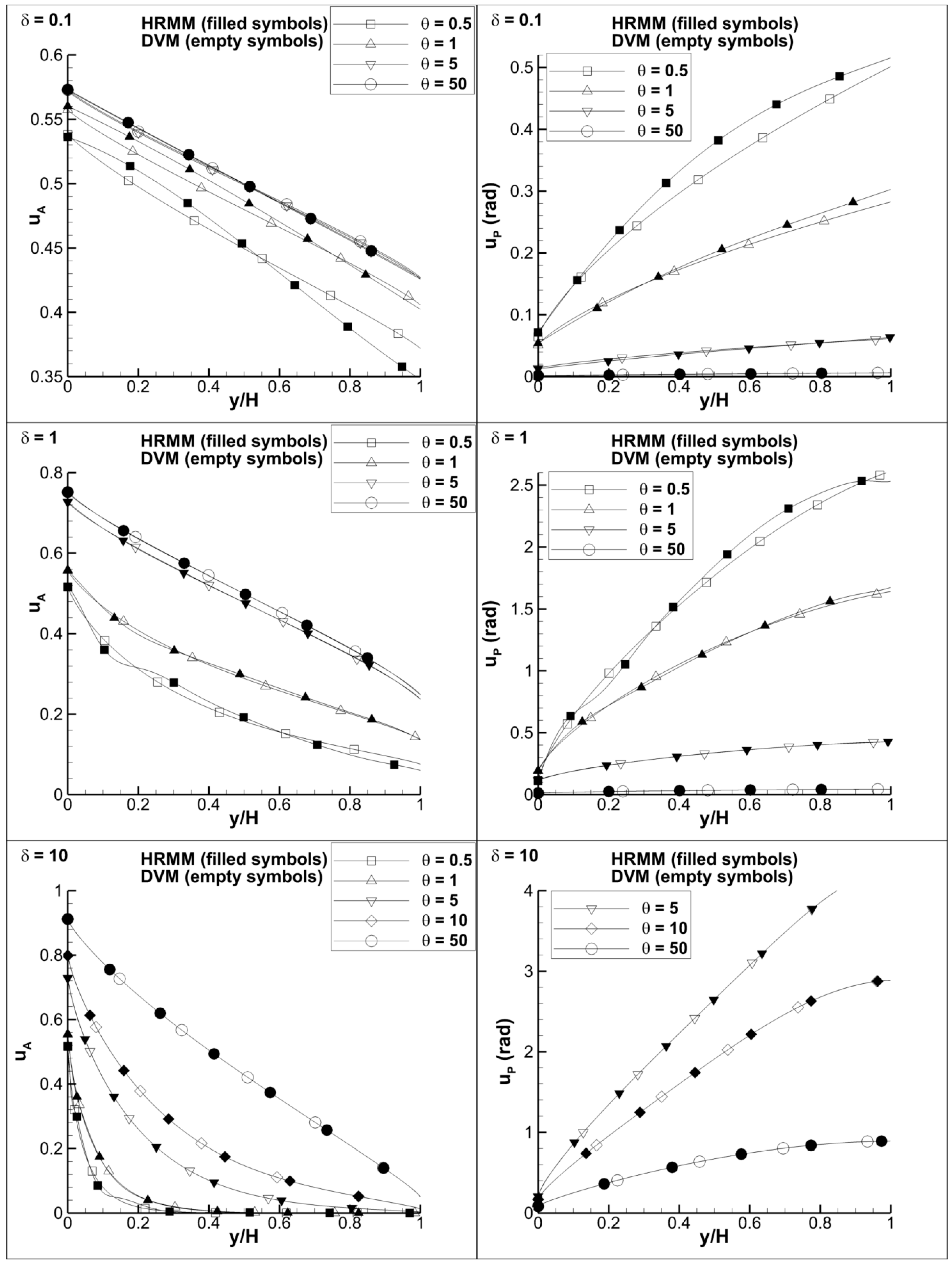
In order to examine the behavior of the HRMM solution in the whole flow domain, in Figure 2, the distributions of the velocity amplitude and phase between the plates are plotted. It is noted that the quantities $u_A\left(y\right)$, $u_P\left(y\right)$ are plotted in terms of $y/H\in \left[0,1\right]$ (instead of $y$) for scaling purposes. The graphs are for the indicative values of $\delta =\left[0.1,1,10\right]$ and $\theta =\left[0.5,1,5,50\right]$. It is noted that at $\delta =10$ and small values of $\theta$, the oscillation is rapidly damped and therefore the associated velocity phases are shown for $\theta =\left[5,10,50\right]$. In general, the agreement between the HRMM and DVM distributions is very good for $\theta =\left[5,10,50\right]$ and then some discrepancies start to appear at $\theta =1$, which are further increased at $\theta =0.5$. Furthermore, the discrepancies become more evident far from the oscillating wall. It may be stated that, as in the case of oscillatory Stokes flow, the present HRMM solution of the oscillatory Couette flow is very accurate at low and moderate frequencies, while it gradually becomes less accurate at high and very high frequencies, not at the oscillating wall but inside the flow domain.

5. Concluding Remarks

A half-range moment method, in terms of the half-range orthogonal Hermite polynomials, for linear oscillatory boundary driven rarefied flows has been constructed. Two flow configurations are used in order to judge the accuracy of the developed scheme, namely the oscillatory Stokes and Couette flows. The former flow (also known as Stokes second problem) is characterized by the oscillation parameter, while the latter one by the oscillation and rarefaction parameters. The computed HRMM results include the amplitude and the phase of the velocity and shear stress distributions for different orders of half-range moments in a wide range of the flow parameters. In the oscillatory Stokes flow the so-called penetration depth is also computed. In all cases a comparison has been performed with corresponding results obtained by the discrete velocity method.

In general, the convergence of the HRMM solution is rapid and a fifth order approximation is very accurate, providing excellent agreement with the corresponding DVM solution at the oscillating plate, as well as in the flow domain. However, at oscillation frequencies of the same or higher order of the collision frequency, discrepancies start to appear in the flow domain. It is believed that these discrepancies are not contributed to the HRMM, which remains valid even in very high oscillation frequencies, but to the solution of the deduced system of half-range moments and may be circumvented by introducing more advanced solvers of ordinary differential equations taking into account the observed spurious oscillations of the solution. In addition, it may be useful to note that these very high oscillation frequencies are mainly of theoretical interest and seldom appear in oscillating systems.

In any case, it has been clearly demonstrated that the half-range moment method can be applied to oscillatory rarefied gas flows providing accurate results in a very wide range of the involved flow parameters. Since the computational effort of the HRMM is negligible, compared to the one of typical computational kinetic type schemes solving for the distribution function itself, it is worthwhile to consider the efficient implementation of the HRMM to stationary and transient multidimensional rarefied gas flows.

References

- Hadjiconstantinou, N.G. Sound wave propagation in transition-regime micro- and nanochannels. Phys. Fluids 2002, 14, 802–809. [Google Scholar] [CrossRef] [Green Version]
- Sharipov, F.; Kalempa, D. Gas flow near a plate oscillating longitudinally with an arbitrary frequency. Phys. Fluids 2007, 19, 017110. [Google Scholar] [CrossRef]
- Sharipov, F.; Kalempa, D. Oscillatory Couette flow at arbitrary oscillation frequency over the whole range of the Knudsen number. Microfluid. Nanofluid. 2008, 4, 363–374. [Google Scholar] [CrossRef]
- Kalempa, D.; Sharipov, F. Sound propagation through a rarefied gas confined between source and receptor at arbitrary Knudsen number and sound frequency. Phys. Fluids 2009, 21, 103601. [Google Scholar] [CrossRef]
- Manelbgka, A.; Hadjiconstantinou, N.G. Gas-flow animation by unsteady heating in a microchannel. Phys. Fluids 2010, 22, 1–12. [Google Scholar]
- Desvillettes, L.; Lorenzani, S. Sound wave resonances in micro-electro-mechanical systems devices vibrating at high frequencies according to the kinetic theory of gases. Phys. Fluids 2012, 24, 1–24. [Google Scholar] [CrossRef] [Green Version]
- Sharipov, F. Rarefied Gas Dynamics; Wiley-VCH Verlag GmbH & Co. KGaA: Weinheim, Germany, 2016. [Google Scholar]
- Emerson, D.R.; Gu, X.J.; Stefanov, S.K.; Yuhong, S.; Barber, R.W. Nonplanar oscillatory shear flow: From the continuum to the free-molecular regime. Phys. Fluids 2007, 19, 107105. [Google Scholar] [CrossRef]
- Gospodinov, P.; Roussinov, V.; Stefanov, S. Nonisothermal oscillatory cylindrical Couette gas flow in the slip regime: A computational study. Eur. J. Mech. B Fluids 2012, 33, 14–24. [Google Scholar] [CrossRef]
- Wu, L.; Reese, J.M.; Zhang, Y. Oscillatory rarefied gas flow inside rectangular cavities. J. Fluid Mech. 2014, 748, 350–367. [Google Scholar] [CrossRef] [Green Version]
- Nassios, J.; Yap, Y.W.; Sader, J.E. Flow generated by oscillatory uniform heating of a rarefied gas in a channel. J. Fluid Mech. 2016, 800, 433–483. [Google Scholar] [CrossRef]
- Yap, Y.W.; Sader, J.E. Sphere oscillating in a rarefied gas. J. Fluid Mech. 2016, 794, 109–153. [Google Scholar] [CrossRef]
- Aoki, K.; Kosuge, S.; Fujiwara, T.; Goudon, T. Unsteady motion of a slightly rarefied gas caused by a plate oscillating in its normal direction. Phys. Rev. Fluids 2017, 2, 1–33. [Google Scholar] [CrossRef]
- Veijola, T. Chapter Fourteen—Gas Damping in Vibrating MEMS Structures. In Micro Nano Technologies; Lindroos, V., Tilli, M., Lehto, A., Motooka, T., Eds.; William Andrew Publishing: Boston, MA, USA, 2010; pp. 259–279. [Google Scholar]
- Manela, A.; Pogorelyuk, L. Cloaking via heating: Approach to acoustic cloaking of an actuated boundary in a rarefied gas. Phys. Fluids 2014, 26, 062003. [Google Scholar] [CrossRef]
- Ben-Ami, Y.; Manela, A. Acoustic field of a pulsating cylinder in a rarefied gas: Thermoviscous and curvature effects. Phys. Rev. Fluids 2017, 2, 093401. [Google Scholar] [CrossRef] [Green Version]
- Ben-Ami, Y.; Manela, A. The sound of a pulsating sphere in a rarefied gas: Continuum breakdown at short length and time scales. J. Fluid Mech. 2019, 871, 668–693. [Google Scholar] [CrossRef]
- Frezzotti, A.; Pietro Ghiroldi, G.; Gibelli, L. Direct solution of the Boltzmann equation for a binary mixture on GPUs. In Proceedings of the AIP Conference Proceedings; American Institute of Physics: Melville, NY, USA, 2011; Volume 1333, pp. 884–889. [Google Scholar]
- Bisi, M.; Lorenzani, S. Damping forces exerted by rarefied gas mixtures in micro-electro-mechanical system devices vibrating at high frequencies. Interfacial Phenom. Heat Transf. 2014, 2, 253–263. [Google Scholar] [CrossRef]
- Bisi, M.; Lorenzani, S. High-frequency sound wave propagation in binary gas mixtures flowing through microchannels. Phys. Fluids 2016, 28, 052003. [Google Scholar] [CrossRef]
- Kalempa, D.; Sharipov, F. Sound propagation through a binary mixture of rarefied gases at arbitrary sound frequency. Eur. J. Mech. B Fluids 2016, 57, 50–63. [Google Scholar] [CrossRef]
- Kalempa, D.; Sharipov, F.; Silva, J.C. Sound waves in gaseous mixtures induced by vibro-thermal excitation at arbitrary rarefaction and sound frequency. Vacuum 2019, 159, 82–98. [Google Scholar] [CrossRef]
- Lorenzani, S. Kinetic modeling for the time-dependent behavior of binary gas mixtures. In AIP Conference Proceedings; AIP Publishing LLC: Melville, NY, USA, 2019; Volume 2132, p. 130006. [Google Scholar]
- Tsimpoukis, A.; Valougeorgis, D. Rarefied isothermal gas flow in a long circular tube due to oscillating pressure gradient. Microfluid. Nanofluid. 2018, 22, 5. [Google Scholar] [CrossRef]
- Tsimpoukis, A.; Valougeorgis, D. Pulsatile pressure driven rarefied gas flow in long rectangular ducts. Phys. Fluids 2018, 30, 047104. [Google Scholar] [CrossRef] [Green Version]
- Tsimpoukis, A.; Vasileiadis, N.; Tatsios, G.; Valougeorgis, D. Nonlinear oscillatory fully-developed rarefied gas flow in plane geometry. Phys. Fluids 2019, 31, 067108. [Google Scholar] [CrossRef] [Green Version]
- Chapman, S.; Cowling, T.G. The Mathematical Theory of Non-Uniform Gases; Cambridge University Press: Cambridge, UK, 1970. [Google Scholar]
- Ferziger, J.H.; Kaper, H.G. Mathematical Theory of Transport Processes in Gases; North-Hollland: Amsterdam, The Netherlands, 1972. [Google Scholar]
- Cercignani, C. Theory and Applications of the Boltzmann Equation; Scottish Academic: Edinburgh, UK, 1975. [Google Scholar]
- Struchtrup, H. Macroscopic Transport Equations for Rarefied Gas Flows; Springer: Berlin/Heidelberg, Germany, 2005. [Google Scholar]
- Grad, H. On the kinetic theory of rarefied gases. Commun. Pure Appl. Math. 1949, 2, 331–407. [Google Scholar] [CrossRef]
- Grad, H. Principles of the Kinetic Theory of Gases. Thermodynamik der Gase/Thermodynamics of Gases; Springer: Berlin/Heidelberg, Germany, 1958; pp. 205–294. [Google Scholar]
- Muller, I.; Ruggeri, T. Rational Extended Thermodynamics. Springer Tracts in Natural Philosophy; Springer: New York, NY, USA, 1998; Volume 37. [Google Scholar]
- Structrup, H.; Torrilhon, M. Regularization of Grad’s 13 moment equations: Derivation and linear analysis. Phys. Fluids 2003, 15, 2688. [Google Scholar] [CrossRef] [Green Version]
- Taheri, P.; Rana, A.S.; Torrilhon, M.; Structrup, H. Macroscopic description of steady and unsteady rarefaction effects in boundary value problems of gas dynamics. Contin. Mech. Thermodyn. 2009, 21, 423. [Google Scholar] [CrossRef]
- Gu, X.J.; Emerson, D.R. Modeling oscillatory flows in the transition regime using a high-order moment method. Microfluid. Nanofluid. 2011, 10, 389–401. [Google Scholar] [CrossRef]
- Lokerby, D.A.; Reese, J.M.; Gallis, M.A. The usefulness of higher-order constitutive relations for describing the Knudsen layer. Phys. Fluids 2005, 17, 100609. [Google Scholar] [CrossRef] [Green Version]
- Torrilhon, M.; Structrup, H. Boundary conditions for regularized 13-moment equations for micro-channel-flows. J. Comput. Phys. 2008, 227, 1982–2011. [Google Scholar] [CrossRef] [Green Version]
- Gross, E.P.; Jackson, E.A.; Ziering, S. Boundary value problems in kinetic theory of gases. Ann. Phys. 1957, 1, 141–167. [Google Scholar] [CrossRef]
- Soga, T. Kinetic analysis of evaporation and condensation in a vapor-gas mixture. Phys. Fluids 1982, 25, 1978–1986. [Google Scholar] [CrossRef]
- Shizgal, B. A Gaussian quadrature procedure for use in the solution of the Boltzmann equation and related problems. J. Comput. Phys. 1981, 41, 309–328. [Google Scholar] [CrossRef]
- Lorenzani, S.; Gibelli, L.; Frezzotti, A.; Frangi, A.; Cercignani, C. Kinetic approach to gas flows in microchannels. Nanoscale Microscale Thermophys. Eng. 2007, 11, 211–226. [Google Scholar] [CrossRef]
- Frezzotti, A.; Gibelli, L.; Franzelli, B. A moment method for low speed microflows. Contin. Mech. Thermodyn. 2009, 21, 495–509. [Google Scholar] [CrossRef]
- Gibelli, L. Velocity slip coefficients based on the hard-sphere Boltzmann equation. Phys. Fluids 2012, 24, 022001. [Google Scholar] [CrossRef]
- Ghiroldi, G.P.; Gibelli, L. A finite-difference lattice Boltzmann approach for gas microflows. Commun. Comput. Phys. 2015, 17, 1007–1018. [Google Scholar] [CrossRef] [Green Version]
- Ambrus, V.E.; Sofonea, V. Half-range lattice Boltzmann models for the simulation of Couette flow using the Shakhov collision term. Phys. Rev. E 2018, 98, 063311. [Google Scholar] [CrossRef] [Green Version]
- Ambrus, V.E.; Sofonea, V. Lattice Boltzmann models based on half-range Gauss-Hermite quadratures. J. Comput. Phys. 2016, 316, 760–788. [Google Scholar] [CrossRef]
- Ambrus, V.E.; Sharipov, F.; Sofonea, V. Comparison of the Shakhov and ellipsoidal models for the Boltzmann equation and DSMC for ab initio-based particle interactions. Comput. Fluids 2020, 211, 104637. [Google Scholar] [CrossRef]
- Busuioc, S.; Ambrus, V.E. Lattice Boltzmann models based on the vielbein formalism for the simulation of flows in curvilinear geometries. Phys. Rev. E 2019, 99, 033304. [Google Scholar] [CrossRef] [Green Version]
- Bhatnagar, P.L.; Gross, E.P.; Krook, M. A Model for Collision Processes in Gases. I. Small Amplitude Processes in Charged and Neutral One-Component Systems. Phys. Rev. 1954, 94, 511–525. [Google Scholar] [CrossRef]
- Sekaran, A.; Varghese, P.; Goldstein, D. An analysis of numerical convergence in discrete velocity gas dynamics for internal flows. J. Comput. Phys. 2018, 365, 226–242. [Google Scholar] [CrossRef]
- Loyalka, S.K.; Petrellis, N.; Storvick, T.S. Some exact numerical results for the BGK model: Couette. Poiseuille and thermal creep flow between parallel plates. Z. Angew. Math. Phys. 1979, 30, 514–521. [Google Scholar] [CrossRef]
- Shi, Y.; Ladiges, D.R.; Sader, J.E. Origin of spurious oscillations in lattice Boltzmann simulations of oscillatory noncontinuum gas flows. Phys. Rev. E 2019, 100, 053317. [Google Scholar] [CrossRef] [PubMed]
Figure 1.
Oscillatory Stokes flow. Comparison between the distributions of velocity and shear stress amplitudes (left) and phases (right) obtained by the half-range moment method (HRMM) () and the discrete velocity method (DVM) for various values of the oscillation parameter.
Figure 2.
Oscillatory Couette flow; comparison between the distributions of velocity amplitudes and phases obtained by HRMM () and the DVM for various values of the oscillation and gas rarefaction parameters.