Monolithic Solvers for Incompressible Two-Phase Flows at Large Density and Viscosity Ratios

Abstract

In this paper, we investigate the accuracy and robustness of three classes of methods for solving two-phase incompressible flows on a staggered grid. Here, the unsteady two-phase flow equations are simulated by finite volumes and penalty methods using implicit and monolithic approaches (such as the augmented Lagrangian and the fully coupled methods), where all velocity components and pressure variables are solved simultaneously (as opposed to segregated methods). The interface tracking is performed with a Volume-of-Fluid (VOF) method, using the Piecewise Linear Interface Construction (PLIC) technique. The home code Fugu is used for implementing the various methods. Our target application is the simulation of two-phase flows at high density and viscosity ratios, which are known to be challenging to simulate. The resulting strategies of monolithic approaches will be proven to be considerably better suited for these two-phase cases, they also allow to use larger time step than segregated methods.

1. Introduction

Understanding the physics of unsteady incompressible two-phase flows at large contrast ratios [1] and their numerical modeling via Navier-Stokes equations has become an important tool that allows understanding further physics of multiphase flows and therefore controls the behavior of these flows in several industrial and environmental applications. However, they remain among the most difficult to simulate numerically for two correlated reasons: the difficulties in the mathematical formalism of these equations resulting from the velocity-pressure coupling [2] and the numerical processing of the interfaces [3] which can be decoupled from solving the Navier-Stokes system. On the one hand, the numerical processing of the interfaces, in particular the interface tracking, which is indispensable for each time iteration, is required for the modeling of discontinuities in physical properties across the interface, in particular in the presence of large density and viscosity ratios, together with the conservation of mass. On the other hand, the main difficulty lies in the linear system that arises from these equations. This is a challenging problem to invert because of (1) the incompressibility constraint that results in a saddle-point structure (zero diagonal pressure block), and (2) large viscosity ratios that strongly couple the velocity components in the interface vicinity.

In the past two decades, much progress has been achieved to treat the different aspects related to the presence of complex shape interfaces and capilary phenomena. On the one hand, Sharp-Interface methods (SIM) considering the interface as a discontinuity, is still the most currently used by the scientific community to deal with two phase-flows. This class of methods fall along to one of the two following approaches: Front Tracking and Front Capturing methods. Front Tracking methods of Tryggvason et al. [4] rely on the Lagrangian advection of a chain of markers connected by segments, where the position of the interface is thus represented by these markers. This method has the advantage of providing an explicit description of the position of the interface, and provides accurate results since it is described at a smaller scale than the mesh associated with the Eulerian velocities (sub-grid resolution). However, problems of connectivity and topology changes make this method difficult to use, especially in 3D. The Interface capturing methods on the other hand consist of capturing the presence of the front directly by using a characteristic phase function. In these approaches, we can cite the level-set method developed by the mathematicians Stanley Osher and James Sethian [5,6], for which a regular description of the interface is used, represented by the zero of a regular function, the signed distance to the interface. Although this method is accurate for the computation of normals and curvature, it does not ensure the mass conservation due to the numerical diffusion of the advection schemes such as the WENO scheme [7], which can cause a modification of the position of the interface. In addition to this, these schemes require the use of a large stencil, which is computationally expensive. Conservative level-set method introduced by Ollson and Kreiss [8,9] is often used, requires the construction of an additional color function, by introducing a diffuse profile via a hyperbolic tangent function. This method conserves the mass of each phase, but require a reinitialization after each advection step. The Volume Of Fluid (VOF) method introduced by Hirt and Nichols [10], use a stiff description of the interface, for which the interface presence is explicitly taken into accout by the volume fraction so called color funtion. The interface location is reconstructed by means of linear approximations in the cells [11]. This method remains very interesting since it allows ensuring a very volume conservation of each phase. However, it suffers from many limitations such as difficult access to the geometric characteristics such as curvatures and normals, and the generation of artificial deformation near the interface when its thickness is of the order of a cell. Finally, the CLSVOF [12] method which involves a coupling between the Level-Set and VOF methods, benefits from the advantages of both these methods. Indeed, the mass is well conserved, and the geometrical properties can be easily calculated. Although these important advantages are important, unfortunately, the implementation of this method remains difficult. A last class of front-capturing method is the Moment Of Fluid method [13] that can be viewed as an extension of the VOF with the addition of the centroid of the phase together with the volume fraction.

Another class of two-flow modeling approach, called the Diffuse Interface Method (DIM), relies on the definition of a physical interfacial thickness whereby the physical properties vary rapidly yet continuously. In the literature, a wide variety of this class of methods has been proposed. These include phase-field methods [14], based on the convection-diffusion equation of the phase, by introducing physical effects that govern interfaces. This method does not require any reinitialization to ensure mass conservation, and has proved also to be very accurate for computing curvature and surface tension forces. Nevertheless, their main drawback it is computationally more expensive, and the mesh size must be small enough to capture the smaller resolved interfacial structures. Another DIM approach is to use the Second Gradient (SG), a technique developed initially by van der Waals [15], and extended for the simulation of liquid-vapor flows with phase change by Didier Jamet [16]. The idea is to propose a smooth variation of the physical properties along the diffuse interface by holding into account the influence of the gradient of the density field and the double gradient of the velocity field. Even if it is challenging to model, this method can yield simulate complex coupled problems. However, both of these interface diffuse methods preserve the interface dynamics through the conservation and give a satisfactory description for the normal and curvatures. It has been demonstrated that at high resolutions, the VOF method yielded higher accuracy at a lower cost compared to diffuse interface methods (see [17]). In this work, our choice was to go with the VOF methods. The remedies for these drawbacks can be circumvented using another class of methods allowing to regularize the VOF. Constrained interpolation profile (CIP) methods of [18], consist of solving hyperbolic equations for the color function. Based on the CIP, the color function and its gradient are calculated to form a cubic interpolation function. This method is known for low numerical diffusivity and good stability. However, its main drawback lies in the interface thickness that is not controlled. A recent regularized VOF method consists in introducing an original smooth volume of fluid function (SVOF) obtained by solving a low cost diffusion equation, as described in [19,20]. This numerical procedure has a priori two advantages. On the one hand, the spread of interfaces through which the physical properties vary strongly but continuously. On the other hand, as the physical properties are continuous, the convergence properties for the fully coupled solver become better, even in the presence of large contrast ratios. In addition, the application of the continuum surface tension force model [21] to SVOF significantly improves the representation of the approximation of surface tension forces.

Furthermore, the treatment of velocity-pressure coupling has been the subject of much work and is a relatively well-controlled problem concerning single-phase flows. On the contrary, in the context of two-phase flow modeling at large density and viscosity ratios, numerical difficulties appear, related to the presence of large interface distortions involving ill-conditioned linear systems. To deal with the velocity-pressure coupling challenge, two strategies can be used: segregated methods introduced independently by Chorin [22] and Temam [23], approximate the original system using time splitting, thereby resulting in two decoupled equations: one to update the velocity field and the other the pressure field although these methods stem from their simplicity and ease of implementation. They still suffer from serious limitations: the splitting operator introduces an error that reduces the temporal accuracy of the numerical solution [24], and the need for pressure boundary conditions that do not exist in the original problem and who are more sensitive to the ratio of densities through the interfaces. The implicit and monolithic approaches such as the augmented Lagrangian (AL) and the fully coupled (FC) methods, solve simultaneously all velocity components and pressure variables, hence preserving the consistency of the discretized system with the continuous equations (while the segregated methods have a time splitting error). The augmented Lagrangian has been developed by Fortin and Glowinski [25] for single-phase Stokes flows and extended by Vincent et al. [26,27] for two-phase flows. The advantages of the augmented Lagrangian method are numerous. The resolution is very robust, and it allows us to simulate a large number of complex unsteady two-phases problems, in which density and viscosity ratio may exceed ${10}^6$. Besides, this approach avoids imposing boundary conditions on the pressure field. The main drawback of the augmented Lagrangian is its numerical expense to achieve low residuals for the inversion of a linear system and divergence levels. Fully coupled methods [28,29,30,31], on the other hand, are purely algebraic, using specific various block preconditioning and Schur complements approximation techniques to solve a saddle point on both fields (velocity and pressure). The resulting strategies, although more difficult to implement and more expensive on a time step basis, prove to be more robust, and very effective for simulating two-phase flows with very large ratios of density and viscosity. They lead to having better convergence properties, with little CFL restrictions.

While the vast majority of related documented studies rely on explicit and segregated methods (such as projection methods), we describe here a fully coupled method for dealing with velocity-pressure coupling, to take advantage of its robustness, principally for the simulation of two-phase flows at large density and viscosity ratios, which has been little studied in the literature. Furthermore, it has been demonstrated that the fully-coupled solver hence preserving the consistency of the discretized system with the continuous equations at large contrast ratio in most cases, which allows to simplify the implementation and to potentially overcome the momentum conserving method contributions (Sussman [32], Raessi [33], Le chenadec [34], Desjardins [35], Ménard [36], …). To characterize the interface location, a PLIC VOF approach is used in the present work. The conclusions arising on solvers would be clearly applicable to level set, CLSVOF, phase field or MOF methods also.

This paper is organized as follows: In Section 2 the Naviers-Stokes equations are formulated for two-phase incompressible flows, and the temporal and spatial discretizations are presented. Section 3 is dedicated to numerical results for two-phase flows to show the advantages of the Fully coupled methods. In Section 4 concluding remarks are drawn.

2. Model and Numerical Methods

2.1. Penalized One-Fluid Model

In the framework of numerical simulation of two-phase incompressible flows involving non-miscible fluids, the one-fluid formulation, developed by Kataoka [37], is considered here. In each of the two fluid phases, the equations to be solved are the conservation of linear momentum, the conservation of volume (the phases are immiscible and incompressible), augmented with the capillary effect. Heat transfer phenomena will be neglected, and therefore we do not have to solve the energy equation. An additional equation will also be solved: the transport equation of a scalar field called the color function.

We consider an open bounded domain $\mathsf{\Omega }\subset {\mathbb{R}}^3$, with boundary $\mathsf{\Gamma }$. Let be $\mathbf{u}$ the fluid velocity, p the pressure field, t the time, $\rho$ the mixture density, $\overline{\overline{T}}$ viscous stress tensor, $\mathbf{f}$ the momentum body force, ${\mathbf{F}}_s$ the capillary term acting on the interface, modeled in this study by the continuum surface tension force model (CSF) [21] and ${\overline{\overline{B}}}_{penu}$ a tensor field for specifying boundary conditions, whose diagonal components tend to infinity along the boundary $\mathsf{\Gamma }$ and are identically zero inside the fluid domain $\mathsf{\Omega }$. The coupling between the one fluid model developped by Kataoka and a penalty method [38] (to treat different types of boundary conditions) give the penalized one-fluid model. In its conservative form, the equations governing the multiphase flow motion then read:

$$\frac{\partial \rho \left(C\right)\mathbf{u}}{\partial t}+\nabla ·\left(\rho \left(C\right)\mathbf{u}\otimes \mathbf{u}\right)+{\overline{\overline{B}}}_{penu}\left(f\left(\mathbf{u}\right)-{\mathbf{u}}_{{}_{\infty }}\right)=-\nabla p+\nabla ·\overline{\overline{T}}+\mathbf{f}+{\mathbf{F}}_s,$$

(1)

$$\nabla ·\mathbf{u}=0,$$

(2)

To characterize the topology of the interface and the fluid properties (mass density and viscosity), the color function C, which vary between 0 and 1, indicates the presence of the interface. It is just advected by the incompressible fluid velocity that is zero divergence under the assumption that no phase change occurs. As previously mentionned, only isothermal incompressible two-phase are considered here. The tracking of the spatio-temporal evolution of the colour function C, requires the resolution of the following advection equation:

$$\frac{\partial C}{\partial t}+\mathbf{u}·\nabla C=0.$$

(3)

To complete the one-fluid formulation, the mixture density $\rho \left(C^s\right)$ and the expression of the viscous stress tensor $\overline{\overline{T}}$ must be specified. As mass is an extensive quantity, the mixture density is defined according to the following constitutive law (arithmetic average, which allows satisfying the conservation of mass intrinsically):

$$\rho \left(C^s\right)={\rho }_1{C}^s+(1-C^s){\rho }_2,$$

(4)

where ${\rho }_1$ and ${\rho }_2$ are the densities of fluid 1 and 2. $C^s$ is the smoothed color function ranging from 0 and 1 as C, whose spread around $C=0.5$ is controlled. This function is obtained by performing a smoothing operation on the color function C by solving the following Helmhotz equation (the reader is referred to [19,20] for more information),

$$\nabla ·D\nabla C^{s,n+1}+C^{s,n+1}=C^{s,n}$$

(5)

where $D=L_i\Delta h^2$ is the diffusion coefficient, which is then defined as the product of the control volume $\Delta h^2$ and a numerical parameter $L_i$. It can be noticed that this parameter allows to ensure that the smoothed color function $C^s$ spans a distance $L_i=k\Delta h$ on either side of the interface, where k is taken between $0.2$ and 2 (see [19,20]). Note that the smoothing operation described above in Equation (5), is equivalent to replacing the interface discontinuity with a zone of adjustable thickness, through which the transition between the two phases has taken place. As a consequence, this method has some advantages. On the one hand, it avoids the generation of artificial deformation near the interface and provides large enough discrete stencils to estimate the normal and the curvature of the interface. On the other hand, using this technique leads to better convergence properties for the implicit solvers, which proves to be more robust, when coping with large viscosity ratios that strongly couple the velocity components in the interface vicinity.

Concerning the viscous stress tensor $\overline{\overline{T}}$, Caltagirone and Vincent [39] proposed a new technique called “Viscous Penalty Method” of second order. The major interest of this formulation is that it allows distinguishing all the physical contributions reflecting the effects of compressibility, elongation, shearing, and rotation. The splitting of these contributions then makes it possible to act differently on each term to strongly impose the associated stress. After suitable decomposition, we assume the viscous stress tensor is given by:

$$\overline{\overline{T}}=\kappa \left(\begin{array}{cc}\frac{\partial u}{\partial x}& 0\\ 0& \frac{\partial v}{\partial y}\end{array}\right)+\zeta \left(\begin{array}{cc}0& \frac{\partial u}{\partial y}\\ \frac{\partial v}{\partial x}& 0\end{array}\right)-\eta \left(\begin{array}{cc}0& \frac{\partial u}{\partial y}-\frac{\partial v}{\partial x}\\ \frac{\partial v}{\partial x}-\frac{\partial u}{\partial y}& 0\end{array}\right)$$

(6)

where $\kappa =2\mu$ for the elongation viscosity, $\zeta =2\mu$ for the shearing viscosity, and $\eta =\mu$ for the rotation viscosity, the evaluation of the viscous operator $\nabla ·\overline{\overline{T}}$ involves in particular the estimates of the elongation viscosity $\kappa =2\mu$ at the pressures nodes, and the pure shearing $\zeta =2\mu$ and rotation $\eta =\mu$ viscosities at the center of the Cartesian grid cells. By using a mixed average for the viscosity, which was initially proposed by Benkenida and Magnaudet [40], and then Vincent et al. [41], the general jump conditions of the momentum equations across the interface are satisfied. In this situation, the diagonal viscous stress is proportional to an elongation viscosity which is determined as a linear function of the smoothed color function called $C^s$,

$${\kappa }_{i,j}=2{\mu }_1{C}_{i,j}^s+2{\mu }_2(1-C_{i,j}^s)$$

(7)

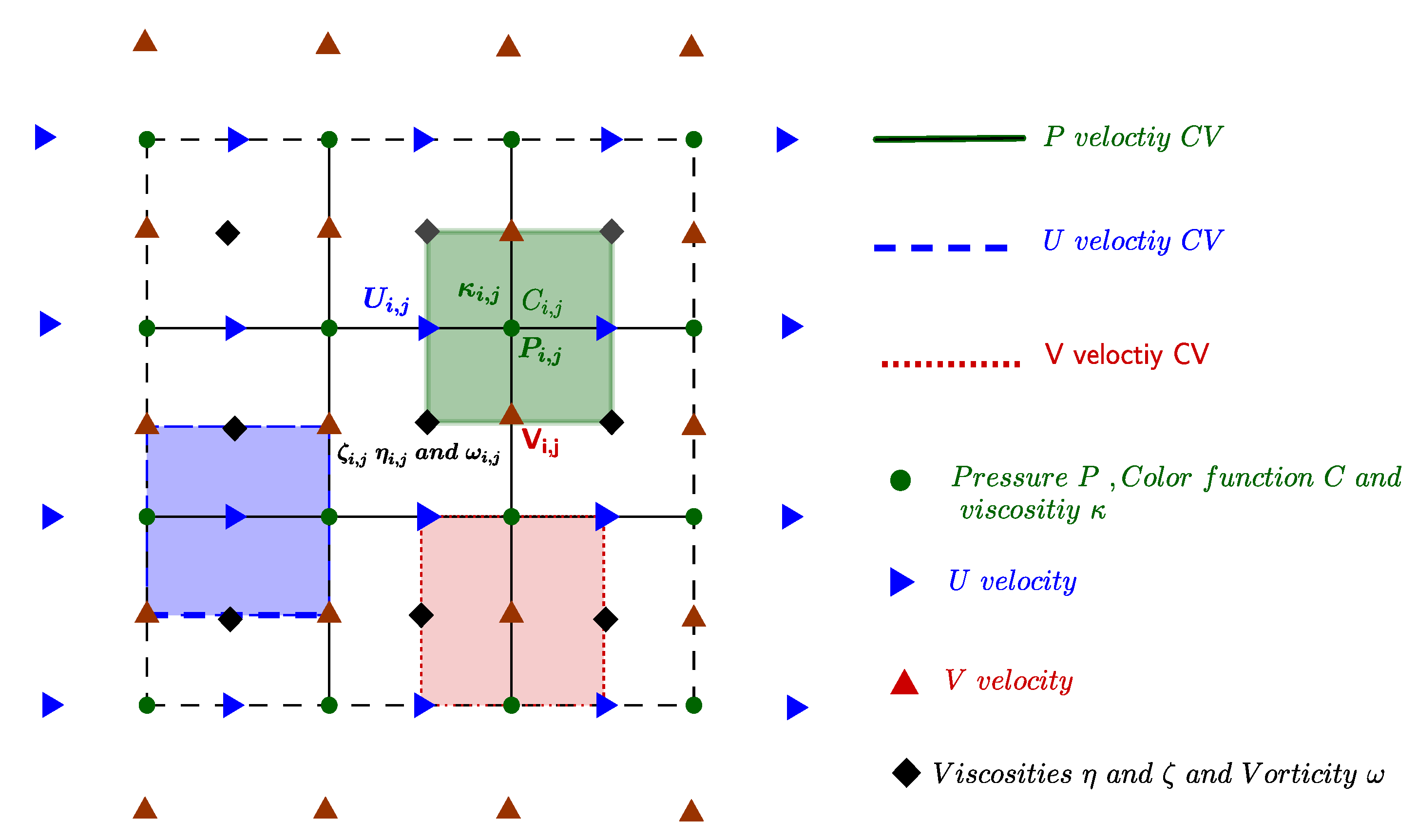
As regards to the off diagonal components of the viscous stress tensor, the pure shearing $\zeta$ and rotation $\eta$ viscosities will be computed by a harmonic average combined with a linear interpolation (Equation (9)) of the adjacent color functions located at the vertices of the cell (see Figure 1), as follows:

$${\zeta }_{i,j}=2{\eta }_{i,j}=2\times \left(\frac{{\mu }_1{\mu }_2}{{\mu }_2{\tilde{C}}_{i,j}^S+{\mu }_1\left(1-{\tilde{C}}_{i,j}^S\right)}\right)$$

(8)

With,

$${\tilde{C}}_{i,j}^S=\frac{C_{i,j}^S+C_{i,j-1}^S+C_{i-1,j}^S+C_{i-1,j-1}^S}{4}$$

(9)

2.2. Discretization Schemes and Solvers

In the present work, the unsteady two-phase flow equations are approximated by finite volumes and penalty methods (to treat different types of boundary conditions), on a staggered mesh according to the MAC scheme of Harlow and Welch [42]. The discrete velocity and pressure variables are located in a staggered way, each having its own control volume, as shown in the Figure 1. This choice guarantees the consistency of the differential operators such as the divergence and the gradient, and it also avoids oscillations on the pressure field. Knowing that the solution of the advection Equation (3) is performed with the VOF method, using the Piecewise Linear Interface Construction (PLIC) technique. The resulting semi-discrete system of mass and momentum conservation equations is advanced in time, implicitly using a second-order integration scheme. In contrast, a centered scheme for the pressure gradient, divergence velocity, convective, and viscous terms is used. To avoid applying the Newton linearization and invert the full Jacobian, which proves more efficient but more expensive for unsteady flow, the convective fluxes are linearized using Adams-Bashforth extrapolation as follows:

$${\mathbf{u}}^{n+1}\otimes {\mathbf{u}}^{n+1}\approx \left(2{\mathbf{u}}^n-{\mathbf{u}}^{n-1}\right)\otimes {\mathbf{u}}^{n+1}.$$

(10)

Here, n refers to a time index associated with physical time $n\Delta t$ and $\Delta t$ is assumed to be the constant time step of each solved iteration. So, after suitable linearization and discretization, and, as an implicit Fully Coupled (FC) resolution is targeted, the generic system is a nonsymmetric linear system of saddle point type which takes the following form:

$$\left(\begin{array}{cc}\frac{1}{\Delta t}{M}_u^{\left(\rho \right)}+N_u^{\left(\rho \right)}+L_u^{\left(\mu \right)}& B_p^T\\ B_u& 0\end{array}\right)\left(\begin{array}{c}{\mathbf{u}}^{n+1}\\ p^{n+1}\end{array}\right)=\left(\begin{array}{c}\mathbf{f}\\ 0\end{array}\right)$$

(11)

or $A\mathbf{x}=\mathbf{b}$. Here, the matrix $B_u$ is the discrete negative divergence and $B_p^T$ represents the discrete pressure gradient operator, $M_u^{\left(\rho \right)}$ is the velocity mass matrix, $L_u^{\left(\mu \right)}$ is the discrete viscous velocity Laplacian, $N_u^{\left(\rho \right)}$ denotes the convective matrix and $\mathbf{f}$ represents the right-hand side vector. Our strategy to solve this sparse linear system is to employ the BiCGStab(2) [43] solver on the entire system, by choosing compressed storage raw (CSR) structure in order to store only the non-null coefficients of the matrix, and then built an efficient preconditioner to accelerate the convergence of the iterative solver. This strategy can be established on the use of pressure convection-diffusion (PCD) preconditioning for the pressure block, and the block Gauss-Seidel preconditioner for the velocity block (See [44] for further details).

3. Numerical Results

As mentioned in the introduction, different approaches have been used to solve the Navier-stokes equations. In the following, we have conducted different simulations of two-phase flow modeling, to demonstrate the accuracy and performance of our new fully coupled solver compared to existing resolution algorithms, and implemented in a home-made code (FUGU) developed at MSME Research Laboratory. The common point of these simulations is that the high density and viscosity ratios seriously complicates the resolution, which constitutes a challenging task.

3.1. Free Fall of Dense Cylindre

The present test case aims at checking the ability of the fully coupled method to simulate multiphase flows with high density and viscosity ratios compared to the standard projection (SP) and adaptative augmented Lagrangian methods. The two-dimensional free fall of a dense cylinder is tested, which has a great interest in having an exact solution but also more severe parameters with high density and viscosity ratios. The initial configuration, consists of a rigid cylinder of radius $r=0.0125\mathrm{m}$, density $\rho ={\rho }_2$ and dynamic viscosity $\mu ={\mu }_2$ which is released without velocity in air. Gravity is set at $g=-9.81\mathrm{m}·{\mathrm{s}}^{-2}$ in the y direction, while the surface tension coefficient $\sigma$ is set to zero. The cylinder is centered at $\left(0.05\mathrm{m},0.15\mathrm{m}\right)$ in a rectangular cavity full of air whose density and viscosity are $\rho ={\rho }_1$ and $\mu ={\mu }_1$ respectively. The cavity is $0.2\mathrm{m}$ high and $0.1\mathrm{m}$ wide. The boundary conditions are slip lateral walls ($\mathbf{u}·\mathbf{n}=\mathbf{0}$) and no-slip on the top and bottom walls ($\mathbf{t}·\left(\nabla \mathbf{u}+{\nabla }^{\mathbf{T}}\mathbf{u}\right)·\mathbf{n}=\mathbf{0}$).

Concerning the numerical parameters, the simulations are carried out on five Cartesian grids (50 × 100, 100 × 200, 200 × 400, and 400 × 800), with a residual of $ϵ={10}^{-6}$ for the BiCGSTAB(2). As far as the time derivatives, a constant time step $\Delta t=6.25\times {10}^{-5}$ s is chosen, and 2300 time steps are computed, corresponding to $0.144$ s of the flow motion. The physical parameters for the test-cases are given in

Table 1. Physical parameters describing the test cases. Here, ${\rho }_2$ and ${\mu }_2$ refers to the fluid density and viscosity respectivly inside the droplet, ${\rho }_1$ and ${\mu }_1$, refers to the density and viscosity of the surrounding fluid respectivly and g is the gravity.

Test Case	${\mathit{\rho }}_1$ [kg· m${}^{-3}$]	${\mathit{\rho }}_2$ [kg· m${}^{-3}$]	${\mathit{\mu }}_1 [\mathbf{Pa}·\mathbf{s}]$	${\mathit{\mu }}_2 [\mathbf{Pa}·\mathbf{s}]$	$\mathit{g} [\mathbf{m}·{\mathbf{s}}^{-2}]$	${\mathit{\rho }}_2/{\mathit{\rho }}_1$	${\mathit{\mu }}_2/{\mathit{\mu }}_1$
1	1.1768	${10}^5$	$1.85\times {10}^{-5}$	${10}^5$	−9.81	${10}^5$	${10}^{10}$

.

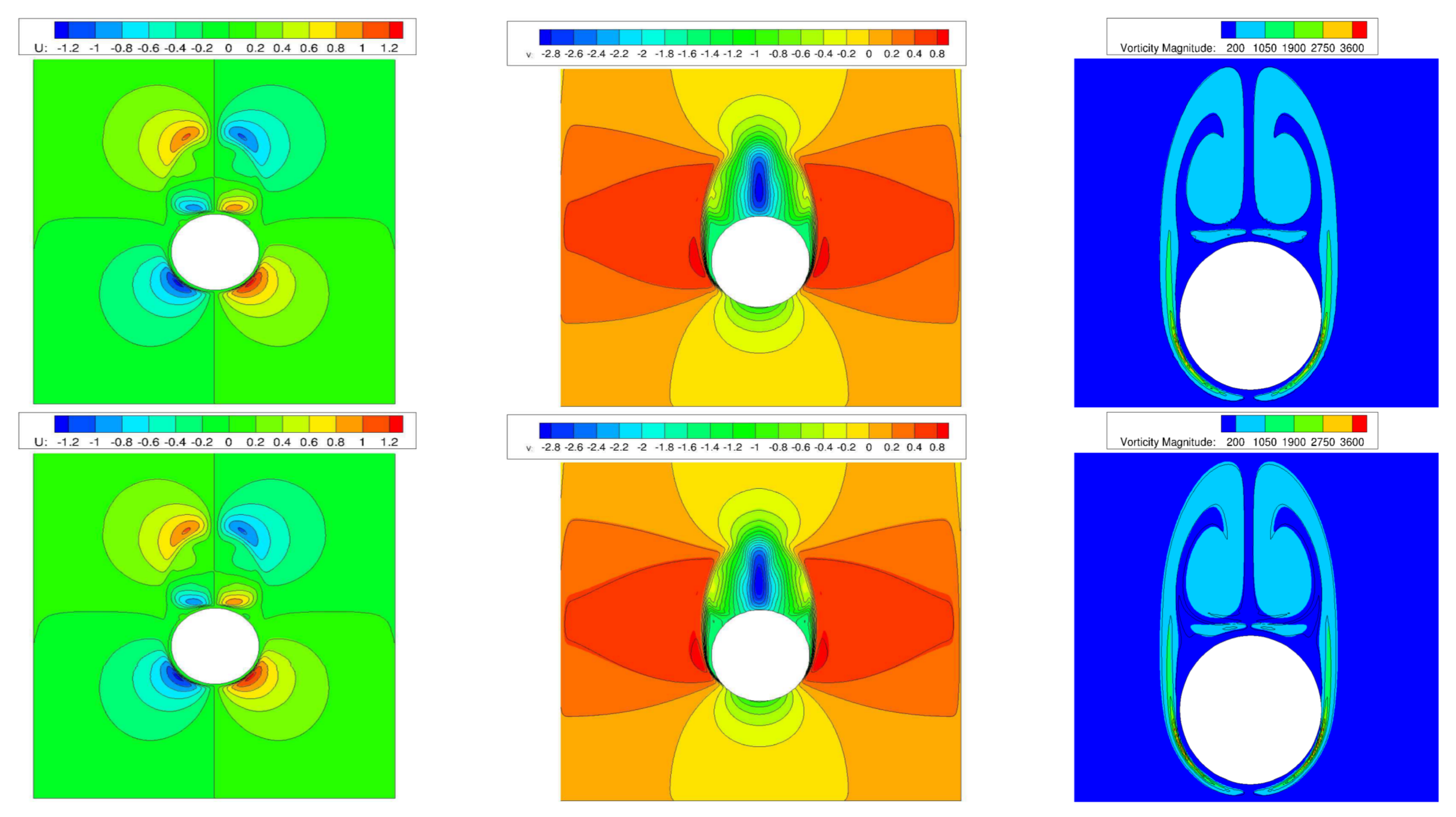
The results obtained by the fully coupled and adaptative augmented Lagrangian solvers are presented in Figure 2 at $t=0.144\mathrm{s}$. It can be seen that these method stays more robust when coping with large viscosity ratios. Hence, a good agreement is observed between both methods, with slight differences in the vorticity fields. Unfortunately, the standard projection method fails to converge towards the end of the simulation because the solver was unable to reach the desired residual to solve the Poisson equation with variable coefficients, and therefore the correction step was not able to reduce the divergence of the predicted velocity. The time step must, therefore, be decreased to ensure a correct quality of numerical solution, performed by the standard projection method. Nevertheless, significant differences can be observed from the field of vorticity magnitude.

3.1.1. Comments on the Falling Velocity and Center of Mass

To evaluate the accuracy of the Fully-coupled method, comparison of results with quantitative and qualitative results are now proposed. To do so, two distinct quantities will be used to describe their temporal evolution. These quantities are defined as follows:

• Center of mass $Y_c$

  $$Y_c=\frac{{\int }_{{\mathsf{\Omega }}_2}y\mathrm{d}x}{{\int }_{{\mathsf{\Omega }}_2}1\mathrm{d}x},$$

  (12)
• Vertical velocity ${\mathbf{U}}_c$

  $${\mathbf{U}}_c=\frac{{\int }_{{\mathsf{\Omega }}_2}\mathbf{U}\mathrm{d}x}{{\int }_{{\mathsf{\Omega }}_2}1\mathrm{d}x}.$$

  (13)

Here $Y_c$ denotes the center of mass of the cylinder, ${\mathbf{U}}_c$ denotes the velocity at the center of mass of the cylinder, and ${\mathsf{\Omega }}_2$ represents the subdomain occupied by the cylinder. Since the exact solution of the falling velocity ($U_c=-gt$) and center of mass ($Y_c=-g{t}^2/2+0.15$) are known, relative errors obtained during this test case can be evaluated using Equation (14).

$$Er{r}_2^{rel}\left(q_t\right)={\left(\frac{{\sum }_{k=1}^{nt}{∥q_t^{ref}-q_t∥}^2}{{\sum }_{k=1}^{nt}{∥q_t^{ref}∥}^2}\right)}^{1/2}$$

(14)

where $q_t^{ref}$ is the reference quantity, $q_t$ is the temporal evolution of quantity q, $nt$ is the number of time steps, n is the mesh refinement level and h the cell size.

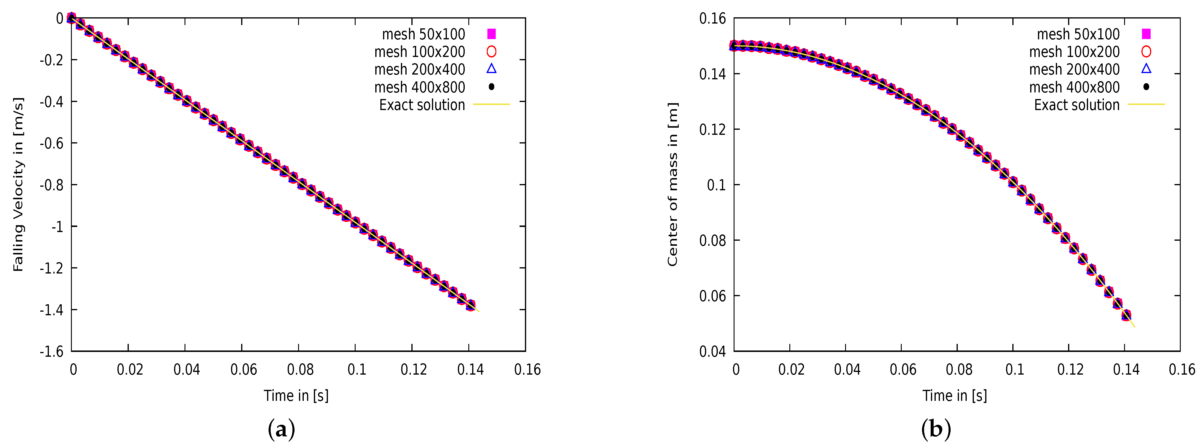
Time evolution of the falling velocity and center of mass are shown in Figure 3 for different grid refinements. This figure demonstrates a clear convergence of the numerical simulations to the exact solution even for coarse grids. The corresponding error between the numerical results and the exact solution is shown in

Table 2. Free fall of a dense cylindre—Values of $Er{r}_2^{rel}\left({\mathbf{U}}_{\mathbf{c}}\right)$ and $Er{r}_2^{rel}\left(Y_c\right)$ according to grid, obtained with Fully-coupled (FC) method, throughout the simulation, after $0.144$ s.

Grid	$\Delta \mathit{t}$	${\mathit{Err}}_2^{\mathit{rel}}\left({\mathbf{U}}_{\mathbf{c}}\right)$	${\mathit{Err}}_2^{\mathit{rel}}\left({\mathit{Y}}_{\mathit{c}}\right)$
$50\times 100$	$6.25\times {10}^{-5}\mathrm{s}$	$5.05\times {10}^{-5}$	$8.41\times {10}^{-4}$
$100\times 200$	$6.25\times {10}^{-5}\mathrm{s}$	$2.37\times {10}^{-5}$	$5.74\times {10}^{-4}$
$200\times 400$	$6.25\times {10}^{-5}\mathrm{s}$	$2.62\times {10}^{-5}$	$2.38\times {10}^{-4}$
$400\times 800$	$6.25\times {10}^{-5}\mathrm{s}$	$3.07\times {10}^{-5}$	$2.21\times {10}^{-4}$

. It is clear from this table that the error level is always low for the fully coupled numerical solutions. Even though errors are saturated (perhaps due to the fact that the simulation are given with a dense and viscous fluid around the cylinder whereas the theory is obtained in vacuum), the results are at least accurate to around $0.01\%$ compared to the exact solution.

In order to be aware of the influence of the numerical methods and their discretization, the results given by the fully coupled method on the finer grid are compared to those of standard projection and adaptative augmented Lagrangian solvers, the performances of each solver are also evaluated. As shown in

Table 3. Free fall of a dense cylindre—Values of $Er{r}_2^{rel}\left({\mathbf{U}}_{\mathbf{c}}\right)$ and $Er{r}_2^{rel}\left(Y_c\right)$ obtained with FC, AAL, and SP at the end of the simulation for $t=0.144\mathrm{s}$, on a grid of size $400\times 800$. NC indicates the simulation stopped due to divergence of the solver.

Method	${\mathit{Err}}_2^{\mathit{rel}}\left({\mathbf{U}}_{\mathbf{c}}\right)$	${\mathit{Err}}_2^{\mathit{rel}}\left({\mathit{Y}}_{\mathit{c}}\right)$	CPU Time in $\left[\mathit{s}\right]$
FC with $\Delta t=6.25\times {10}^{-5}\mathrm{s}$	$5.05\times {10}^{-5}$	$2.21\times {10}^{-4}$	44,986
AAL with $\Delta t=6.25\times {10}^{-5}\mathrm{s}$	$6.63\times {10}^{-5}$	$1.25\times {10}^{-4}$	101,933
SP with $\Delta t=6.25\times {10}^{-5}\mathrm{s}$	NC	NC	-
SP with $\Delta t=6.25\times {10}^{-6}\mathrm{s}$	$3.36\times {10}^{-5}$	$7.05\times {10}^{-5}$	486,941

, the error levels are comparable for the Fully-coupled and augmented Lagrangian solver for the same time step $\Delta t=6.25\times {10}^{-5}\mathrm{s}$. However, the fully coupled solver is faster because it saves 56% of the CPU time compared to the adaptative augmented Langrangian. These large differences can be explained by the fact that the augmented Lagrangian takes a lot of iterations to converge, with a saturation of the BiCG-Stab(2) solver. Furthermore, the use of a very large value of the parameter r is required to satisfy the incompressibility constraint. This leads to an ill-conditioned linear system, hence inducing the high cost of the augmented Lagrangian method. This is in contrast with the projection method, which requires a time step ten times smaller than other methods to obtain the same quality of solution. This choice seems reasonable in order to reduce the numerical dissipation due to splitting operators. However, this brings the standard projection method to be the most expensive in CPU time.

3.1.2. Comments on the Enstrophy

The enstrophy is a crucial integral quantity that is associated to dissipation and the effects of small-scale turbulence. It has to be noted that a two-dimensional work is perfomed here and that in two-dimensions, the energy cascade that coud be related to turbulence and enstrophy is different from what occurs in three dimensions. Mathematically, the enstrophy is defined as the integral of vorticity square over the domain, and it will be written as $En{s}_1$ for fluid 1:

$$En{s}_1={\int }_V^{}\frac{{\omega }^2}{2}\mathrm{d}V$$

(15)

where $\omega =\left(\frac{\partial v}{\partial x}-\frac{\partial u}{\partial y}\right)$ is the vorticity in two dimensions. The following discrete analog of the enstrophy $En{s}_1$ is used, in wich ${\tilde{C}}_{i,j}$ is the color function located at the viscosities nodes (${\tilde{C}}_{i,j}=0$ in fluid 1 and ${\tilde{C}}_{i,j}=1$ in fluid 2).

$$En{s}_1\simeq \sum _{i,j}^{}\left(1-{\tilde{C}}_{i,j}\right)\frac{{\omega }_{i,j}^2}{2}\Delta V$$

(16)

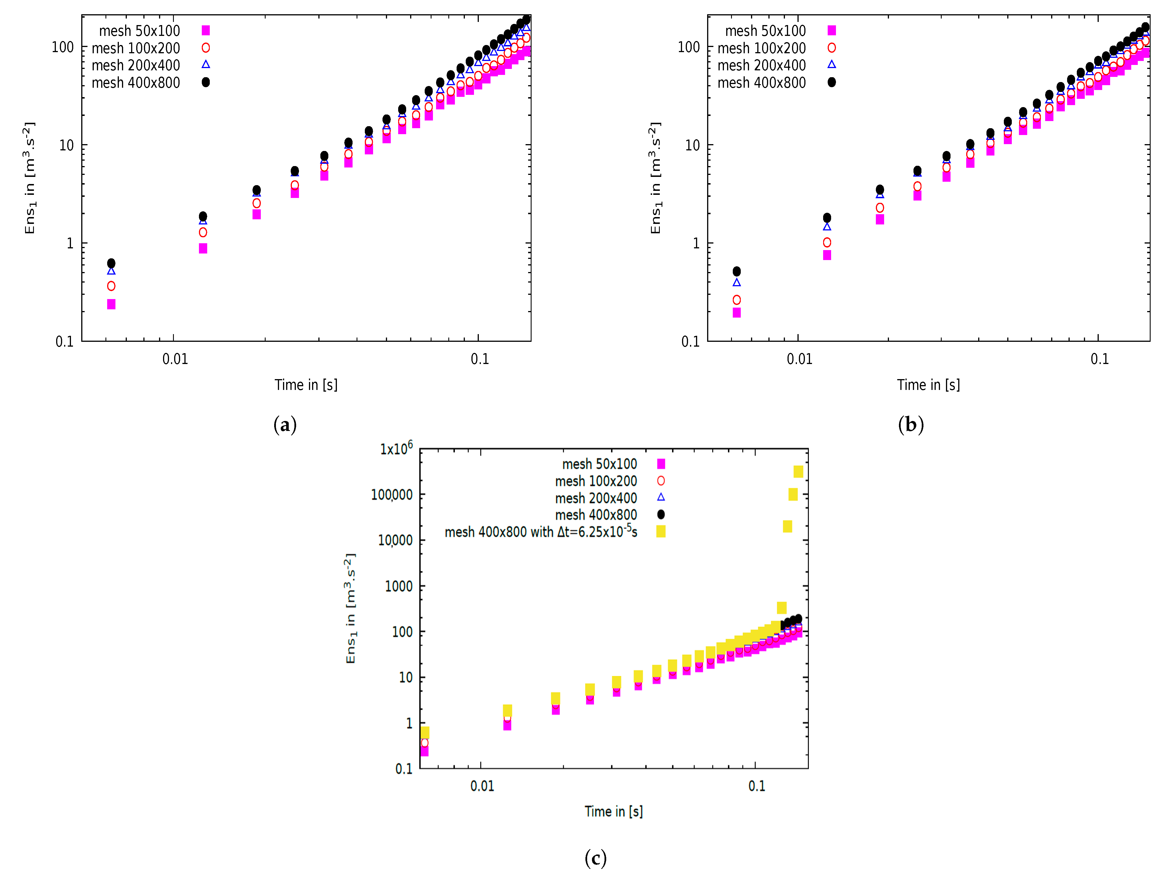
In this part, the evolution of the enstrophy in fluid 1 is investigated, for different grid sizes and test cases as in the previous study. The results are illustrated in Figure 4 on a logarithmic scale, for different grid sizes. As can be seen in this figure, the enstrophy increases over time in a monotonous way. As far as the convergence of the enstrophy, the $200\times 400$ grid simulation is enough to converge the enstrophy for the fully coupled and the adaptative augmented Lagrangian solvers. In contrast, the enstrophy diverges on the finer grid for the standard projection, for the same reasons as the one mentioned before. And a time step ten times smaller is then needed to obtain the same solutions as the exact solvers (fully coupled and adaptative augmented Lagrangian solvers).

3.2. Liquid Sheet Atomisation

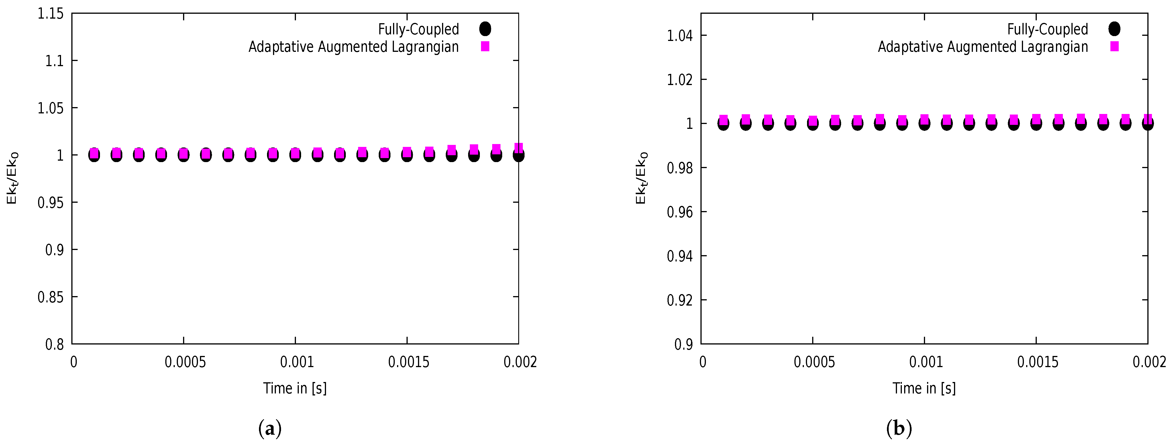
To demonstrate the efficiency and robustness of the monolithic solvers for preserving kinetic energy, a flow interacting with a liquid sheet of thickness $\delta =3\times {10}^{-4}\mathrm{m}$ is investigated [45]. This problem is defined in two dimensions on a square domain of side $L=3\times {10}^{-3}\mathrm{m}$ with periodic and symmetry boundary conditions for the horizontal and vertical sides of the domain, respectively. Simulations are carried out on a $256\times 256$ Cartesian grids with a density ratio of 100 and 1000, while viscosity and capillary forces are set to zero, in order to preserve the initial kinetic energy during the simulation. The initial velocity field is defined as:

$$U=\left\{\begin{array}{c}u=A-0.04cos\left(\frac{2\pi x}{L}\right)\frac{L}{2\pi }\frac{-2}{\delta }{e}^{-\frac{2y}{\delta }}\hfill \\ v=0.04sin\left(\frac{2\pi x}{L}\right)e^{-\frac{2y}{\delta }}\hfill \end{array}\right.$$

(17)

$$A=\left\{\begin{array}{c}30{\mathrm{m}·\mathrm{s}}^{-1}inthegas\hfill \\ 2{\mathrm{m}·\mathrm{s}}^{-1}intheliquid\hfill \end{array}\right.$$

(18)

The results of the time evolutions of the kinetic energy are reported in Figure 5 for all density ratios. It can be observed that whatever the density ratio, the total kinetic energy obtained by the fully coupled solver is conserved over time to almost computer error, which is in good agreement with the theory. As regard to the adaptative augmented Lagrangian solver, a slight increase in the kinetic energy is noticed here but the results are encouraging. On the contrary, the standard projection crashes after a few time iterations even for very small time steps. Consequently, the kinetic energy diverges due to the numerical dissipation generated by the splitting of operators. Besides, it has been shown that the conserving momentum method improves the conservation of the kinetic energy until the interface begins to deform. After this instant, kinetic energy decreases with projection methods, as reported for example in the work of Mukundan et al. [45]. On the other hand, these interfacial instabilities appear more quickly for the classic WENO and conservative Weno schemes. In this work, a centered scheme with either Fully Coupled or Augmented Lagrangian techniques conserves the kinetic energy for longer times compared to existing methods in the literature without the apparence of interfacial instabilities, which is an interesting result allowing to encourage more researchers to work with the monolithic solvers.

3.3. Simulation of 2D Viscous Jet Buckling

The jet buckling problem is an essential phenomen since it is involved in many industrial applications such as the food industry or the aeronautics and aerospace applications with the filling of rocket boosters with propergol. The corresponding flow conditions are at low Reynolds number. This problem has been studied initially by Tomé et al. [46], who have provided a physical criterion which establishes the experiments with buckling jets. Then many numerical investigations [47,48,49] have been conducted to simulate this problem in 2d and 3d configurations, for which the computational results are compared with experiments. The interest of this case lies in two reasons: on the one hand, the possibility of comparing the numerical solutions with experimental ones. On the other hand, the strong viscosity and density gradients near the interface yield ill-conditioned linear systems, which is a task challenge at the algebraic level. For numerical simulations, a square cavity of side $L=1\mathrm{m}$ full of gas is considered. In its upper part, a highly viscous fluid is injected at inlet velocity and inlet width equal to $-1{\mathrm{m}·\mathrm{s}}^{-1}$ and $D=0.08\mathrm{m}$, respectively, while the gravitational force acts with a constant intensity $g=9.81{\mathrm{m}·\mathrm{s}}^{-2}$ in the negative y-direction. For boundaries, a slip wall is employed on the solid walls and outflow boundary conditions at the outlet in the upper part of the cavity, outside the injector. The characteristics of the simulations are given in

Table 4. Physical parameters describing the test cases. Here, ${\rho }_2$ and ${\mu }_2$ refer to the propergol density and viscosity respectivly, ${\rho }_1$ and ${\mu }_1$, refer to the density and viscosity of the gas respectivly, $Re=\frac{{\rho }_{2}D{V}_0}{{\mu }_2}$ is the Rynolds number associated to the propergol, $\frac{H}{D}$ is the aspect ratios of the jet and $V_0$ is the inlet velocity. In the present work, propergol (fluid 2) is assumed to behave like a Newtonian fluid, for the sake of simplicity.

Test Case	${\mathit{\rho }}_1 [\mathbf{kg}·{\mathbf{m}}^{-3}]$	${\mathit{\rho }}_2 [\mathbf{kg}·{\mathbf{m}}^{-3}]$	${\mathit{\mu }}_1 [\mathbf{Pa}·\mathbf{s}]$	${\mathit{\mu }}_2 [\mathbf{Pa}·\mathbf{s}]$	$\mathbf{Re}$	$\frac{\mathit{H}}{\mathit{D}}$	${\mathit{V}}_0 [\mathbf{m}·{\mathbf{s}}^{-1}]$	${\mathit{\rho }}_2/{\mathit{\rho }}_1$	${\mathit{\mu }}_2/{\mathit{\mu }}_1$
1	1.1768	1800	$1.85\times {10}^{-3}$	500	$0.1728$	$12.5$	$0.6$	1529	$1.6\times {10}^5$
2	1.1768	1800	$1.85\times {10}^{-3}$	300	$0.6$	10	1	1529	$2.7\times {10}^5$
3	1.1768	1800	$1.85\times {10}^{-3}$	300	$3.6$	10	6	1529	$2.7\times {10}^5$

:

In their study, Tomé et al. give two important parameters to ensure the occurrence of buckling: the aspect ratios of the jet $H/D>3\pi$ and $Re<0.52$, where $Re$ is the Reynolds number based on the inflow diameter D and the velocity inlet $V_0$. Thus, the objective of this study is to compare the performance of three methods (the fully-coupled, adaptative augmented Lagrangian, and the standard projection) to deal with this kind of problem and to provide a good prediction of their associated physical behavior whereby the matrices resulting from discretization will be solved with the same solver, the BiCGSTAB(2) with a residual of $ϵ={10}^{-6}$.

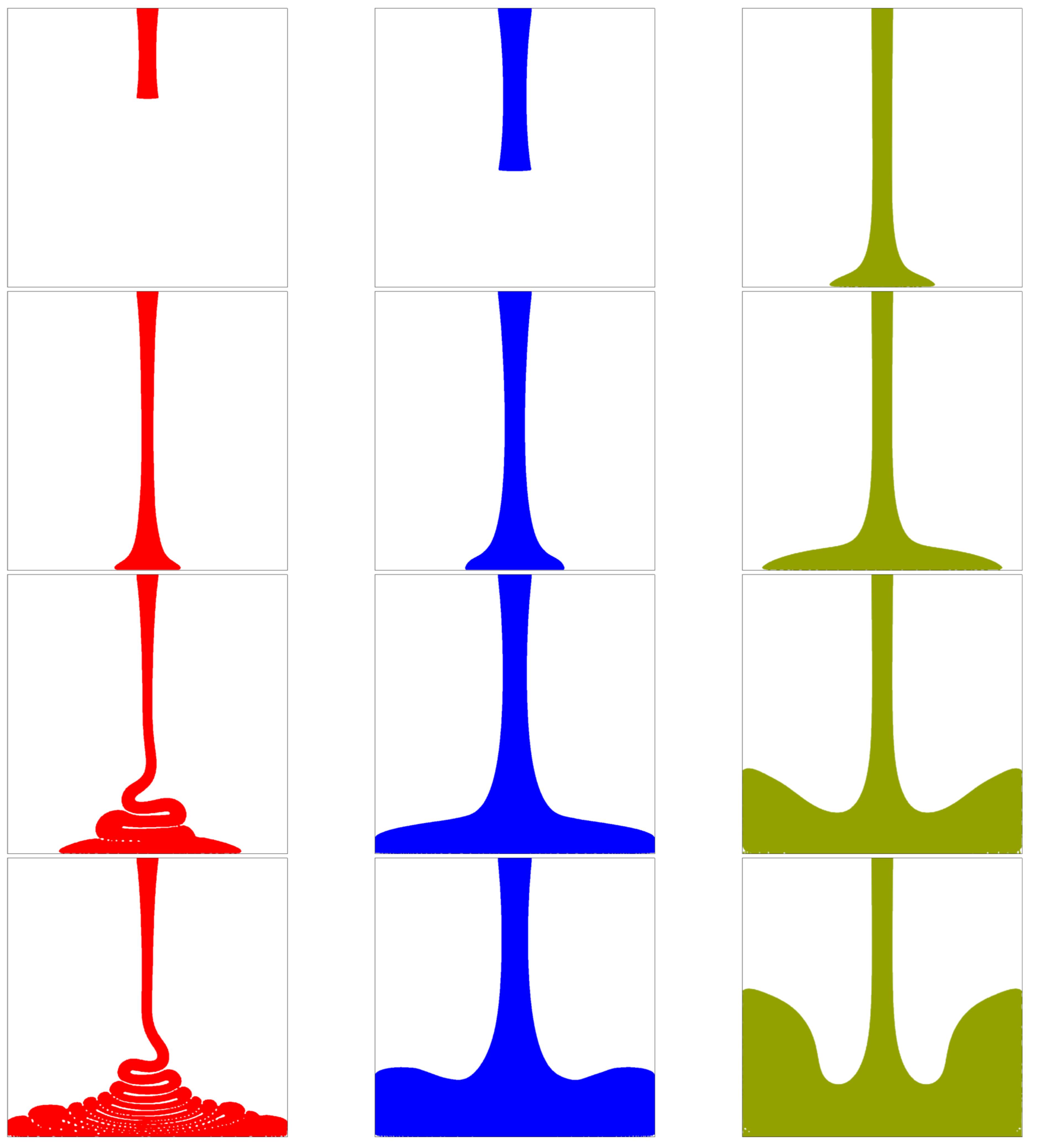
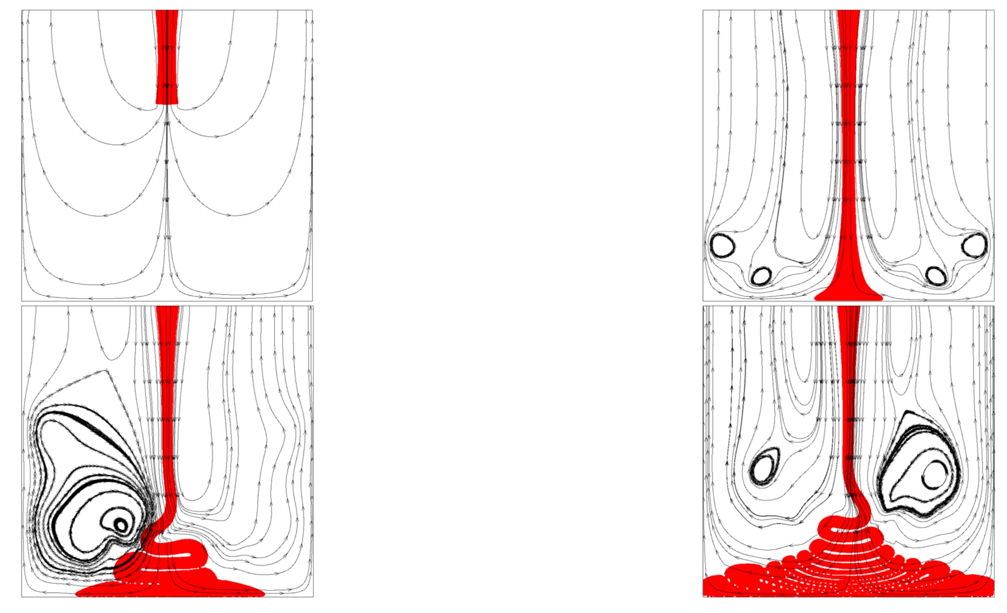
First the evolution of the liquid over time is considered for three Reynolds numbers $Re=0.1728$, $Re=0.6$ and $Re=3.6$ (see Figure 6) using a $320\times 320$ Cartesian grid and a time step $\Delta t=5\times {10}^{-4}\mathrm{s}$. From these figures, It is noticeable that the numerical calculations with the fully-coupled method provide excellent results for the physics of the jet, which are in good agreement with the theoretical criterion given in [46]. Indeed, the first case $Re=0.1728$ corresponds to a buckling jet, whereas second and third cases (also in first case for short times), $Re=0.6$ and $Re=3.6$ the jet oscillation does not appear. In the first case, it is observed that the diameter of the jet decreases in the middle part of the cavity, but the jet remains symmetric, this is because no buckling occurs. On the contrary, in the first case, as soon as it hits the lower wall of the cavity, the jet destabilizes, and helicoïdal instability develops and traps air bubbles in the coiling motion of the viscous fluid. Finally, the streamlines are shown in Figure 7 for the first case, which gives the possibility to evaluate the interaction of both flows. From these figures, recirculations are observed, the size of which increases and then decreases alternately with the oscillations of the jet.

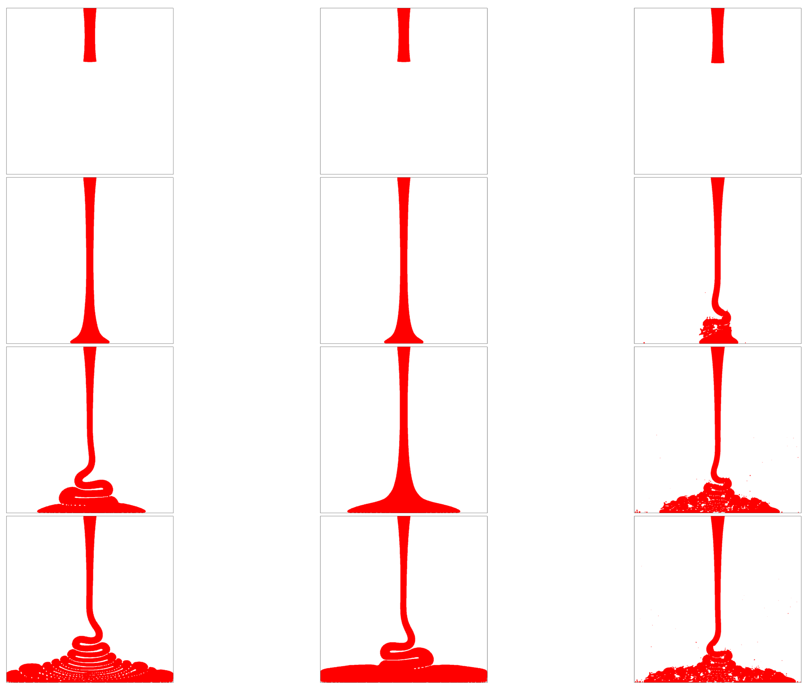
The results obtained with the adaptative augmented Lagrangian method are presented in Figure 8 for $Re=0.1728$, using also a $320\times 320$ Cartesian grid and a time step $\Delta t=5\times {10}^{-4}\mathrm{s}$. The computation shows coherence between the fully coupled and the adaptative augmented Lagrangian methods at times $t=1\mathrm{s}$ and $t=2\mathrm{s}$. Then, significant differences are noticed because the instability did not occur at the same time as with the fully coupled method, due to the nature of the augmented Lagrangian parameter, which behaves like a viscosity. These differences are also due to the unstable nature of the flow that amplifies numerical erros differently in accordance with the difference of the solvers that are not sensitive similarly to truncation errors. The good point is that they trigger an instability for the same Re and in the relevant injection situation. However, it has been seen that the standard projection method for $Re=0.1728$ on $320\times 320$ mesh, fails to converge after 2800 iterations because the correction step was not able to reduce the divergence of the predicted velocity. The cases of $Re=0.6$ and $Re=3.6$ were simulated with the adaptative augmented Lagrangian and the standard projections methods. However, in these cases, all methods give the same results as those of the fully coupled method.

4. Conclusions

A monolithic solver for simulating incompressible two-phase flows, at large density and viscosity ratios, has been develloped and coupled with a VOF method such as PLIC technique. The coupled strategies belong to the two distinct classes of methods: the adaptative augmented Lagrangian method and the fully-coupled solver. These were chosen in order to overcome the difficulties associated with the segregated methods (such as projection methods). This allowed us to simulate complex cases characterized by high density and viscosity ratios, such as the free fall of dense cylindre and the viscous jet buckling, but also to potentially overcome the momentum conserving method in the case of Liquid sheet atomisation. We have also shown that this monolithic solvers allow to use larger time steps than segregated methods, which fails to converge in some cases. In future work, it will be intented to investigate fully coupled solvers on complex 3D and on a massively parallel computers.

References

- Nangia, N.; Griffith, B.E.; Patankar, N.A.; Bhalla, A.P.S. A robust incompressible Navier-Stokes solver for high density ratio multiphase flows. J. Comput. Phys. 2019, 390, 548–594. [Google Scholar] [CrossRef] [Green Version]
- Guermond, J.; Minev, P.; Shen, J. An overview of projection methods for incompressible flows. Comput. Methods Appl. Mech. Eng. 2006, 195, 6011–6045. [Google Scholar] [CrossRef] [Green Version]
- Mirjalili, S.; Jain, S.; Dodd, M. Interface-Capturing Methods for Two-Phase Flows: An Overview and Recent Developments; Annual Research Brief; Center for Turbulence Research: Stanford, CA, USA, 2017; pp. 117–135. [Google Scholar]
- Tryggvason, G.; Bunner, B.; Esmaeeli, A.; Juric, D.; Al-Rawahi, N.; Tauber, W.; Han, J.; Nas, S.; Jan, Y.J. A Front-Tracking Method for the Computations of Multiphase Flow. J. Comput. Phys. 2001, 169, 708–759. [Google Scholar] [CrossRef] [Green Version]
- Osher, S.; Sethian, J. Fronts propagating with curvature-dependent speed: Algorithms based on Hamilton-Jacobi formulations. J. Comput. Phys. 1988, 79, 12–49. [Google Scholar] [CrossRef] [Green Version]
- Bonito, A.; Nochetto, R.H. (Eds.) Chapter 6—A review of level set methods to model interfaces moving under complex physics: Recent challenges and advances. In Handbook of Numerical Analysis; Elsevier: Amsterdam, The Netherlands, 2020; Volume 21, pp. 509–554. [Google Scholar]
- Jiang, G.S.; Shu, C.W. Efficient Implementation of Weighted ENO Schemes. J. Comput. Phys. 1996, 126, 202–228. [Google Scholar] [CrossRef] [Green Version]
- Olsson, E.; Kreiss, G. A conservative level set method for two phase flow. J. Comput. Phys. 2005, 210, 225–246. [Google Scholar] [CrossRef]
- Olsson, E.; Kreiss, G.; Zahedi, S. A conservative level set method for two phase flow II. J. Comput. Phys. 2007, 225, 785–807. [Google Scholar] [CrossRef]
- Hirt, C.; Nichols, B. Volume of fluid (VOF) method for the dynamics of free boundaries. J. Comput. Phys. 1981, 39, 201–225. [Google Scholar] [CrossRef]
- Youngs, D. Time-Dependent Multi-material Flow with Large Fluid Distortion. Numer. Methods Fluid Dyn. 1982, 24, 273–285. [Google Scholar]
- Sussman, M.; Puckett, E.G. A Coupled Level Set and Volume-of-Fluid Method for Computing 3D and Axisymmetric Incompressible Two-Phase Flows. J. Comput. Phys. 2000, 162, 301–337. [Google Scholar] [CrossRef] [Green Version]
- Ahn, H.; Shashkov, M.; Christon, M. The Moment-of-Fluid Method in Action. APS 2007, 60, KB-003. [Google Scholar] [CrossRef]
- Ding, H.; Spelt, P.; Shu, C. Diffuse interface model for incompressible two-phase flows with large density ratios. J. Comput. Phys. 2007, 226, 2078–2095. [Google Scholar] [CrossRef]
- van der Waals, J.D. Thermodynamische Theorie der Kapillarität unter Voraussetzung stetiger Dichteänderung. Z. Phys. Chem. 1894, 13U, 657–725. [Google Scholar]
- Jamet, D.; Lebaigue, O.; Coutris, N.; Delhaye, J. The Second Gradient Method for the Direct Numerical Simulation of Liquid—Vapor Flows with Phase Change. J. Comput. Phys. 2001, 169, 624–651. [Google Scholar] [CrossRef]
- Mirjalili, S.; Ivey, C.B.; Mani, A. Comparison between the diffuse interface and volume of fluid methods for simulating two-phase flows. Int. J. Multiph. Flow 2019, 116, 221–238. [Google Scholar] [CrossRef] [Green Version]
- Sato, Y.; Ničeno, B. A conservative local interface sharpening scheme for the constrained interpolation profile method. Int. J. Numer. Methods Fluids 2012, 70, 441–467. [Google Scholar] [CrossRef]
- Pianet, G.; Vincent, S.; Leboi, J.; Caltagirone, J.P.; Anderhuber, M. Simulating compressible gas bubbles with a smooth volume tracking 1-Fluid method. Int. J. Multiph. Flow 2010, 36, 273–283. [Google Scholar] [CrossRef]
- Guillaument, R.; Vincent, S.; Caltagirone, J.P. An original algorithm for VOF based method to handle wetting effect in multiphase flow simulation. Mech. Res. Commun. 2015, 63, 26–32. [Google Scholar] [CrossRef]
- Brackbill, J.; Kothe, D.; Zemach, C. A continuum method for modeling surface tension. J. Comput. Phys. 1992, 100, 335–354. [Google Scholar] [CrossRef]
- Chorin, A.J. Numerical Solution of the Navier-Stokes Equations. Math. Comput. 1968, 22, 745–762. [Google Scholar] [CrossRef]
- Témam, R. Sur l’approximation de la solution des équations de Navier-Stokes par la méthode des pas fractionnaires (I). Arch. Ration. Mech. Anal. 1969, 32, 135–153. [Google Scholar] [CrossRef]
- Guermond, J.L. Remarques sur les méthodes de projection pour l’approximation des équations de Navier-Stokes. Numer. Math. 1994, 67, 465–473. [Google Scholar] [CrossRef]
- Fortin, M.; Glowinski, R. Augmented Lagrangian Methods: Applications to the Numerical Solution of Boundary-Value Problems. ZAMM J. Appl. Math. Mech. Z. Angew. Math. Mech. 1985, 65, 622. [Google Scholar]
- Vincent, S.; Caltagirone, J.P.; Lubin, P.; Randrianarivelo, T.N. An adaptative augmented Lagrangian method for three-dimensional multi-material flows. Comput. Fluids 2004, 33, 1273–1289. [Google Scholar] [CrossRef]
- Vincent, S.; Sarthou, A.; Caltagirone, J.; Sonilhac, F.; Février, P.; Mignot, C.; Pianet, G. Augmented Lagrangian and penalty methods for the simulation of two-phase flows interacting with moving solids. Application to hydroplaning flows interacting with real tire tread patterns. J. Comput. Phys. 2011, 230, 956–983. [Google Scholar] [CrossRef] [Green Version]
- Benzi, M.; Golub, G.H.; Liesen, J. Numerical solution of saddle point problems. Acta Numer. 2005, 14, 1–137. [Google Scholar] [CrossRef] [Green Version]
- Elman, H.C.; Silvester, D.J.; Wathen, A.J. Finite Elements and Fast Iterative Solvers: With Applications in Incompressible Fluid Dynamics; Oxford University Press: Oxford, UK, 2005. [Google Scholar]
- Bootland, N.; Bentley, A.; Kees, C.; Wathen, A. Preconditioners for Two-Phase Incompressible Navier–Stokes Flow. SIAM J. Sci. Comput. 2019, 41, B843–B869. [Google Scholar] [CrossRef] [Green Version]
- Cai, M.; Nonaka, A.J.; Bell, J.B.; Griffith, B.E.; Donev, A. Efficient Variable-Coefficient Finite-Volume Stokes Solvers. Commun. Comput. Phys. 2014, 16, 1263–1297. [Google Scholar] [CrossRef] [Green Version]
- Bussmann, M.; Kothe, D.B.; Sicilian, J.M. Modeling High Density Ratio Incompressible Interfacial Flows. Volume 1: Fora, Parts A and B; 2002; pp. 707–713. Available online: http://xxx.lanl.gov/abs/https://asmedigitalcollection.asme.org/FEDSM/proceedings-pdf/FEDSM2002/36150/707/4546310/707_1.pdf (accessed on 27 December 2020).
- Raessi, M.; Pitsch, H. Consistent mass and momentum transport for simulating incompressible interfacial flows with large density ratios using the level set method. Comput. Fluids 2012, 63, 70–81. [Google Scholar] [CrossRef]
- Le Chenadec, V.; Pitsch, H. A monotonicity preserving conservative sharp interface flow solver for high density ratio two-phase flows. J. Comput. Phys. 2013, 249, 185–203. [Google Scholar] [CrossRef]
- Desjardins, O.; Moureau, V.; Pitsch, H. An accurate conservative level set/ghost fluid method for simulating turbulent atomization. J. Comput. Phys. 2008, 227, 8395–8416. [Google Scholar] [CrossRef]
- Asuri Mukundan, A.; Ménard, T.; Herrmann, M.; Motta, J.; Berlemont, A. Analysis of dynamics of liquid jet injected into gaseous crossflow using proper orthogonal decomposition. In Proceedings of the AIAA SciTech 2020 Forum, Orlando, FL, USA, 6–10 January 2020. [Google Scholar] [CrossRef]
- Kataoka, I. Local instant formulation of two-phase flow. Int. J. Multiph. Flow 1986, 12, 745–758. [Google Scholar] [CrossRef]
- Angot, P.; Bruneau, C.H.; Fabrie, P. A penalization method to take into account obstacles in viscous flows. Numer. Math. 1999, 81, 497–520. [Google Scholar] [CrossRef]
- Caltagirone, J.P.; Vincent, V. Sur une méthode de pénalisation tensorielle pour la résolution des équations de Navier-Stokes. Comptes Rendus De L’Académie Des Sci. Ser. IIB Mech. 2001, 329, 607–613. [Google Scholar] [CrossRef]
- Benkenida, A.; Magnaudet, J. Une méthode de simulation d’écoulements diphasiques sans reconstruction d’interfaces. Comptes Rendus De L’Académie Des Sci. Ser. IIB Mech. Phys. 2000, 328, 25–32. [Google Scholar] [CrossRef]
- Vincent, S.; de Motta, J.C.B.; Sarthou, A.; Estivalezes, J.L.; Simonin, O.; Climent, E. A Lagrangian VOF tensorial penalty method for the DNS of resolved particle-laden flows. J. Comput. Phys. 2014, 256, 582–614. [Google Scholar] [CrossRef] [Green Version]
- Harlow, F.H.; Welch, J.E. Numerical Calculation of Time-Dependent Viscous Incompressible Flow of Fluid with Free Surface. Phys. Fluids 1965, 8, 2182–2189. [Google Scholar] [CrossRef]
- Dongarra, J.J.; Duff, I.S.; Sorensen, D.C.; Van der Vorst, H.A. Numerical Linear Algebra for High Performance Computers; Society for Industrial and Applied Mathematics: Philadelphia, PA, USA, 1998. [Google Scholar]
- Elouafa, M.; Vincent, S.; Le Chenadec, V. Navier-Stokes Solvers for Incompressible Single-and Two-Phase Flows. Working Paper Accepted in CiCP Journal. Available online: https://hal-upec-upem.archives-ouvertes.fr/hal-02892344/document (accessed on 27 December 2020).
- Mukundan, A.A.; Ménard, T.; de Motta, J.C.B.; Berlemont, A. A 3D Moment of Fluid method for simulating complex turbulent multiphase flows. Comput. Fluids 2020, 198, 104364. [Google Scholar] [CrossRef] [Green Version]
- Tomé, M.F.; Duffy, B.; McKee, S. A numerical technique for solving unsteady non-Newtonian free surface flows. J. Non-Newton. Fluid Mech. 1996, 62, 9–34. [Google Scholar]
- Vincent, S.; Caltagironel, J.P. Efficient solving method for unsteady incompressible interfacial flow problems. Int. J. Numer. Methods Fluids 1999, 30, 795–811. [Google Scholar] [CrossRef]
- Xu, X.; Ouyang, J.; Jiang, T.; Li, Q. Numerical simulation of 3D-unsteady viscoelastic free surface flows by improved smoothed particle hydrodynamics method. J. Non-Newton. Fluid Mech. 2012, 177–178, 109–120. [Google Scholar] [CrossRef]
- Oishi, C.; Martins, F.; Tomé, M.; Alves, M. Numerical simulation of drop impact and jet buckling problems using the eXtended Pom—Pom model. J. Non-Newton. Fluid Mech. 2012, 169–170, 91–103. [Google Scholar] [CrossRef]
Figure 1.
Staggered pressure and velocity unknowns in the global domain. the pressure , the elongation viscosity and the colour function are located at the nodes of the Eulerian grid, the horizontal velocity is defined on the left and right sides of the control volume (in green) associated with and vertical velocity is defined on the bottom and top sides of the control volume associated with , the vorticity , and the rotational and shear viscosities are located at the vertices of the control volume associated with .
Figure 2.
Free fall of dense cylinder at s, obtained on a fine mesh by the three methods. In the first row, FC (shown by fields) and AAL (by isolines). In the second row, FC (shown by fields) and SP (by isolines with s). The different fields presented in each row are: left horizontal velocity , middle: vertical velocity , and right: vorticity magnitude .
Figure 3.
Vertical velocity and center of mass for test case 1 obtained by the fully coupled method with several meshes. (a) Vertical velocity and (b) center of mass.
Figure 4.
Time evolution of enstrophy in fluid 1 for the free fall of dense cylindre case. Obtained by several numerical methods with several Cartesian mesh. (a) FC method, (b) AAL method and (c) SP method.
Figure 5.
Time evolution of normalized kinetic energy for the high density ratio periodic Liquid sheet. Results obtained by different numerical methods, where (a) density ratio is 1000 and (b) density ratio is 100.
Figure 6.
Numerical simulation of a viscous liquid (propergol) jet injected in a square cavity on a grid: the interface is plotted at time , and (first row), , and (second row), , and (third row) and , and (fourth row). First column , second column and third column . Simulations are carried out wit hthe FC method.
Figure 7.
Numerical simulation of a viscous liquid (propergol) jet injected in a square cavity on a grid: the interface is plotted at time and (first row), and (second row). Test case 1 corresponds to .
Figure 8.
Numerical simulation of a viscous liquid (propergol) jet injected in a square cavity on a grid: the interface is plotted at time (first row), (second row), (third row) and (fourth row). First column (FC method), second column (AAL method) and third column (SP method).