On the Use of a Domain Decomposition Strategy in Obtaining Response Statistics in Non-Gaussian Seas


1
Department of Civil Engineering, Faculty of Engineering Science, KU Leuven, Kasteelpark Arenberg 40, B-3001 Leuven, Belgium
2
Department of Infrastructure Engineering, Melbourne School of Engineering, The University of Melbourne, Parkville, VIC 3010, Australia
*
Author to whom correspondence should be addressed.
†
These authors contributed equally to this work.
Fluids 2021, 6(1), 28; https://0-doi-org.brum.beds.ac.uk/10.3390/fluids6010028
Submission received: 28 November 2020
/
Revised: 22 December 2020
/
Accepted: 5 January 2021
/
Published: 7 January 2021
(This article belongs to the Special Issue Selected Papers from the 15th OpenFOAM Workshop)
Abstract
:During recent years, thorough experimental and numerical investigations have led to an improved understanding of dynamic phenomena affecting the fatigue life and survivability of offshore structures, e.g., ringing and springing and extreme wave impacts. However, most of these efforts have focused on modeling either selected extreme events or sequences of highly nonlinear waves impacting offshore structures, possibly overestimating the actual load to be experienced by the structure. Overall, not much has been done regarding short-term statistics. Although clear non-Gaussian statistics and therefore higher probabilities of extreme waves have been observed in random seas due to wave–wave interaction phenomena, which can impact short-term statistics for the structural load, they have not been studied extensively regarding the assessment of the dynamic behavior of offshore structures. Computational fluid dynamics (CFD) models have shown their viability for studying wave–structure interaction phenomena. Despite the continuously increasing computational resources, these models remain too computationally demanding for applications to the large spatial domains and long periods of time necessary for studying short-term statistics of non-Gaussian seas. Higher-order spectral (HOS) models, on the other hand, have been proven to be efficient and adequate in studying non-Gaussian seas. We therefore propose a one-way domain decomposition strategy, which takes full advantage of the recent advances in CFD and of the computational benefits of HOS. When applying this domain decomposition strategy, it appeared to be possible to deduce response statistics regarding the impact of nonlinear wave–wave interactions.
1. Introduction
Due to the world’s ever-growing energy demand, the offshore wind industry has known an exponential growth during the last two decades. As a result, there is a strong tendency towards increasingly larger wind turbines being constructed offshore and cost-reduction per kilowatt hour, which poses new challenges regarding design and efficiency [1,2]. XL-monopiles are one such example. Offshore wind turbines have grown increasingly taller and are installed in deeper water depths than ever before, which jeopardizes their fatigue life due to a higher susceptibility to ringing and springing as their natural frequencies decrease further towards typical wave frequencies [3]. Moreover, innovative structures combining wave energy take-off and harvesting wind energy, e.g., combined offshore wind and offshore airborne prototypes, confront designers with substantial differences in dynamic behavior compared to traditional structures stemming from the oil and gas industry. Especially in terms of prevailing fluid phenomena, viscous effects and turbulence gain considerable importance when assessing such structures.
Traditionally, design practices adopt Gaussian seas to represent operational conditions, while real seas are non-Gaussian [4]. In modeling moderately severe wave climates, second-order wave theory is adopted, which gives rise to increased dynamic response for both stiff and compliant structures due to bound second-order wave components [5]. However, in addition to bound components, free wave components are known to interact at third order of nonlinearity for intermediate to deep water wave conditions, which results in spectral energy downshifts and a higher probability of extremes compared to second-order wave theory [6,7]. Due to these spectral energy downshifts, the dynamic response of stiff structures is reduced [8], while at the same time increased probability for extreme events, due to focussing, could lead to a higher occurrence of transient dynamic phenomena, such as ringing and slamming. An improved understanding of the influence of these nonlinear wave–wave interactions on the response statistics could therefore lead to a more appropriate assessment of offshore structures in operational conditions.
Expensive physical experiments in large-scale facilities and simplified engineering models originating from the offshore industry are still the norm. Most numerical models resolve the Euler equations, assuming incompressibility, irrotationality and inviscosity. Moreover, a Taylor expansion around the water level is used to approximate the kinematic and dynamic atmospheric boundary conditions imposed for the wave dynamics problem. As a result, linear potential theory based models, e.g., NEMOH, and expansions up to second-order, e.g., WAMIT, are still of main use, which is a clear consequence of offshore activities being situated in deep water, where second-order theory is generally assumed to capture most phenomena. However, as bottom-founded structures are situated closer to shore and higher-order wave effects, e.g., ringing, originate from higher-order wave harmonics, these models do not suffice in assessing state-of-the-art innovative offshore structures. Therefore, extensive research has been done in recent years to resolve the wave dynamics boundary value problem with fully nonlinear boundary conditions. Two such efforts are the nonlinear potential flow solvers OceanWave3D and formulations of the higher-order spectral equations (HOS). While OceanWave3D is essentially a fully nonlinear potential flow model [9], HOS solves the Euler equations up to a desired level of nonlinearity in the (spectral) wave number domain [10,11]. By truncating up to third-order nonlinearity, HOS has shown to accurately capture the effect of nonlinear four-wave interactions on extreme wave statistics [12]. Nonetheless, all of the aforementioned models still lack in the sense that they do not model viscosity nor turbulence.
As computational fluid dynamics (CFD) solves the full Reynolds-averaged Navier–Stokes (RANS) equations, it overcomes the problems previously posed by the Euler based models, therefore allowing for viscosity and turbulent effects to be taken along [13]. CFD accurately captures the wave–structure interaction, even in highly nonlinear waves. A notable code is the open-source CFD solver OpenFOAM, of which different branches exist and to which researchers worldwide contribute. Notwithstanding the continuously growing computational resources, these models remain computationally demanding, which makes for a real challenge in applying them to large, high resolution domains and long computational times. Consequently, CFD is often used in conjunction with faster models as part of a domain decomposition approach.
In Paulsen et al. [14,15], such a domain decomposition approach was adopted to model respectively wave impact and ringing for monopiles, where the previously mentioned fully nonlinear potential flow solver OceanWave3D as far-field was used in conjunction with OpenFOAM modeling the near-field through coupling by the wave generation and (passive) absorption toolbox waves2Foam. At the near-field boundaries, numerical relaxation zones, which gradually force the computated wave field to comply with the theoretical wave field calculated through the fully nonlinear far-field solver, were applied [16]. A similar strategy was applied in studying breaking of rogue waves arising from modulational instability in a wave train consisting of a carrier wave and side-band perturbations, where a domain decomposition was adopted between the higher-order spectral model (HOSM) and OpenFOAM. First, an initial wave train was simulated in HOSM until a certain threshold for wave height was reached. Subsequently, this wave surface was fed to the wave maker in the wave generation and (active) absorption toolbox olaFlow to closely study the breaking, for which HOSM does not account [17]. More recently, adopting CFD for both the far field and near field, Di Paolo et al. [18] presented a coupling approach with a 2D CFD model representing the far field and a 3D CFD model for the near field, foregoing the limitations associated with potential flow models. However, adopting this approach would still be too time-consuming in studying long time series, as is the case in this work, and CFD also invokes inaccuracies in its long-distance progressive wave modeling [19].
Alternatively, in Luquet et al. [20], field decomposition through the Spectral Wave Explicit Navier-Stokes Equations (SWENSE) approach has been proposed as a way of coupling the computationally efficient HOS solver to fully nonlinear wave tanks. First, the flow field potential is decomposed into the HOS potential and the near field solution in the numerical wave tank. Next, after evaluating the HOS potential, the nonlinear wave tank potential is solved for with the HOS potential as free surface boundary condition. Finally, adding both potentials produces the full flow field potential. SWENSE therefore allows for fast parallellized computations for both the far field solutions in HOS and the near field solutions in numerical wave tanks. In the OpenFOAM branch, foam-extend, this very same strategy has been successfully implemented together with similar passive absorption boundary conditions as in Jacobsen et al. [16] to prevent waves from reflecting into the near field. In doing so, both extreme wave simulations and the accurate assessment of near field effects on the structure have become possible [21,22]. However, although this approach is very effective in obtaining realistic extreme waves arising from an initial wave field and in studying their impacts on offshore structures, HOS essentially resolves the time evolution of an initial wave field. Therefore, this approach is as such less suited for deriving structural response statistics regarding the spatial evolution of random seas and the nonlinear wave–wave interactions involved, which have shown to lead to a departure from Gaussian statistics [7,23].
This work presents an efficient numerical strategy in generating sufficient data to assess the effect of the interacting free wave components on the response of a stiff monopile. The response statistics for a simple offshore structure in non-Gaussian seas are studied in the time domain. To this end, an efficient domain decomposition strategy, where the near field is modeled through CFD and the far field through a fast HOS numerical wave tank model, is adopted. The purpose of this work is to show that such a domain decomposition strategy is an effective and efficient way to study the response characteristics of a structure under wave loads. In the following, first, the methodology of the domain decomposition strategy is discussed. Next, the set-up and numerical input of far field, near field and structural test case are laid out. Based on the thus established models, a benchmark study for the domain decomposition strategy with emphasis on convergence is presented, after which, the simplified structural model’s validity is assessed. Finally, a discussion takes place considering the ability of the developed time domain approach regarding response statistics in non-Gaussian seas, proving that the model is able to live up to expectations, but, however efficient, still becomes too expensive in view of the multiple long Monte Carlo simulations needed for the response statistics to be representative.
2. Methodology
2.1. Domain Decomposition
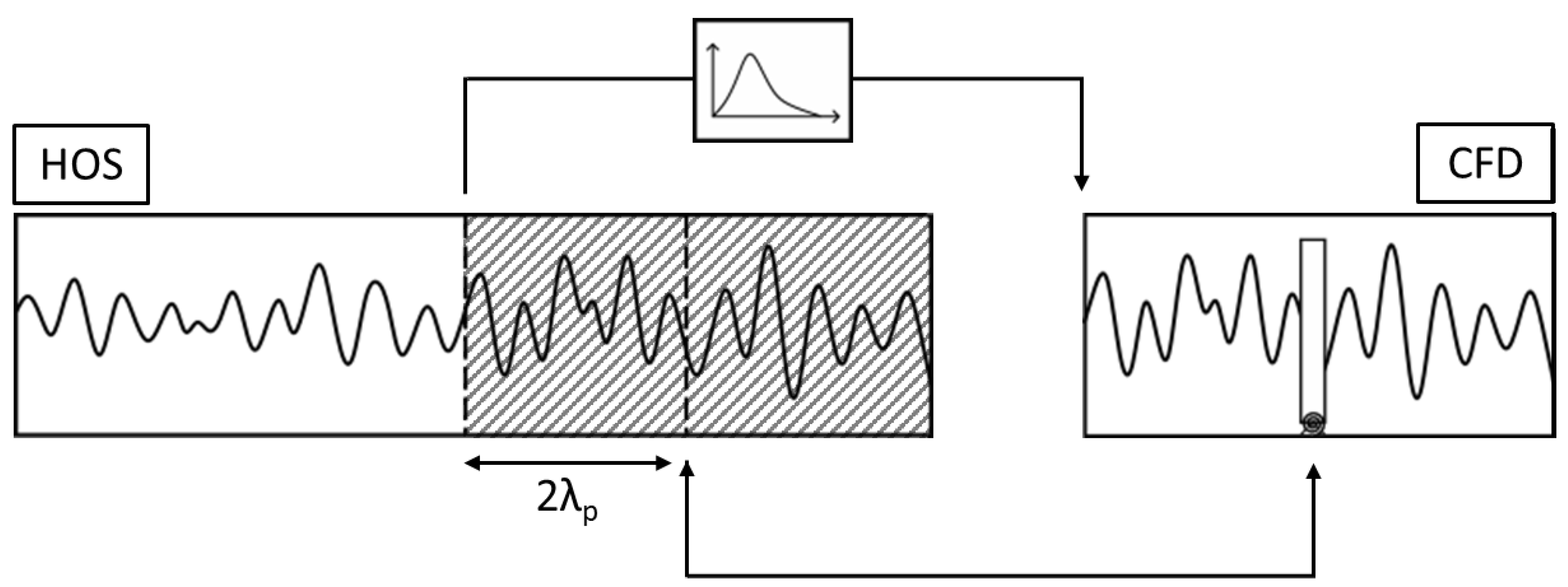
Previous work by Toffoli et al. [23] showed that a large amount of randomly generated (deep) water waves are needed to obtain reliable response statistics regarding nonlinear wave–wave interactions. Moreover, these waves have to travel over long distance to attain their nonlinear properties, when starting from an initial wave field composed of a random superposition of linear waves. If and when maximum non-Gaussianity is reached is primarily related to , with k the wave number and d the water depth. For deep water waves this typically occurs after about 10–15 wavelengths, while for intermediate water depths (), where monopiles are typically built, convergence is not reached even after 20 wavelengths, as will be illustrated further on. As the computational cost of using a full CFD model would be excessive, the domain decomposition strategy, demonstrated in Figure 1 is applied. As shown in Figure 1, the fluid domain is decomposed into a far field modeled by HOS and a near field accounted for by the CFD solver, OpenFOAM [24].
In the domain decomposition strategy, HOS is used to randomly generate a time series by a wave maker boundary first. In previous work by Toffoli et al. [7,23], the higher-order spectral method (HOSM), has shown to yield statistically significant results regarding the influence of third-order nonlinearities on the occurrence of extreme waves in random wave fields. The higher-order spectral implementation typically resolves the Laplace equations in cyclic wave number space with nonlinear free surface boundary conditions formulated in Equations (1) and (2) with and respectively the vertical velocity and the velocity potential at the free surface, [25].
Starting from a randomly generated initial wave field, HOSM then uses a series expansion to resolve the wave surface up to desired order of nonlinearity [11].
The higher-order spectral numerical wave tank, HOS-NWT, by Ducrozet et al. [26], is selected to obtain the spatial evolution of a wave field generated by a wave-making boundary. As a numerical wave tank domain is finite by definition and necessitates the presence of wave generation and absorption boundary conditions, HOS-NWT, adopts an additional velocity potential in an approach similar to what was done in Luquet et al. [20] to account for these boundary conditions. Similarly, as is the case for traditional HOS codes, no wave breaking models or dissipation have been implemented into the publicly available code [27], so that when breaking should occur, i.e., if the steepness exceeds a limit, the computation breaks down.
After running HOS-NWT, the input time series for the near field numerical wave basin in OpenFOAM is determined by taking the wave gauge corresponding to maximum kurtosis and assuming this probe to be the equivalent position of the structure in the near field OpenFOAM model. Subsequently, the time series measured at a wave gauge two peak wavelengths back, i.e., the distance between the wave generation boundary and the structure in the near field numerical modeling is then reconstructed by the olaFlow wave generation and absorption toolbox from the measured spectrum and used as boundary for the near field model.
Assuming incompressibility and irrotationality, the continuity and momentum equations in respectively Equations (3) and (4) together with the two-phase mixture continuity in Equation (5) are then solved by OpenFOAM’s interFoam solver.
In Equation (4), the hydrostatic pressure relates to the total pressure p as , and depicts a vector coefficient used for volume-of-fluid compression in Equation (5). represents the dynamic viscosity, the water density and the water volume fraction bounded between 0 and 1.
Before applying the measured wave spectrum to the near field boundary, the high frequencies in the HOS-NWT solution need to be filtered. The reason is two-fold. On the one hand, these high-frequencies are unphysical in the sense that they do not lie within the frequency range typically associated with wind-generated waves. On the other hand, when applying an unfiltered wave field including these high-frequency components as boundary condition to the near field, it jeopardizes numerical stability at the inlet. Moreover, including very low-frequency wave components might lead to an increasing water level in the CFD model. A low-frequency cut-off is therefore adopted as well. Filtering only retains energy in the frequency range from 0.33 to 3, with the peak wave frequency of the applied spectrum, which still includes the phenomena of interest for the simplified monopile herein considered. However, in case of compliant structures, a smaller low-frequent cut-off wave frequency might be considered to trigger the slow structural responses, while stiffer structures will define the high-frequent cut-off wave frequency.
As a first assessment regarding the applicability of the proposed domain decomposition model in obtaining response statistics for offshore structures in non-Gaussian seas, a simplified structural model is added to the wave flume after benchmarking the coupled approach’s ability to reproduce the HOS wave field. A monopile-founded offshore wind turbine modeled as a 1 DoF inverted pendulum with a spring-damper hinge aimed at approaching the first fore-aft bending frequency, is chosen. Due to the small excursions of the monopile in the water fraction, a one-way coupled approach, where waves impact on a fixed monopile to then apply the thus obtained wave loads in a structural solver, would also be acceptable. However, the inverted pendulum model also served the purpose of verifying mesh motion for a simple structure before transgressing to more complex multi-degrees-of-freedom motion.
2.2. A Simplified Structural Model
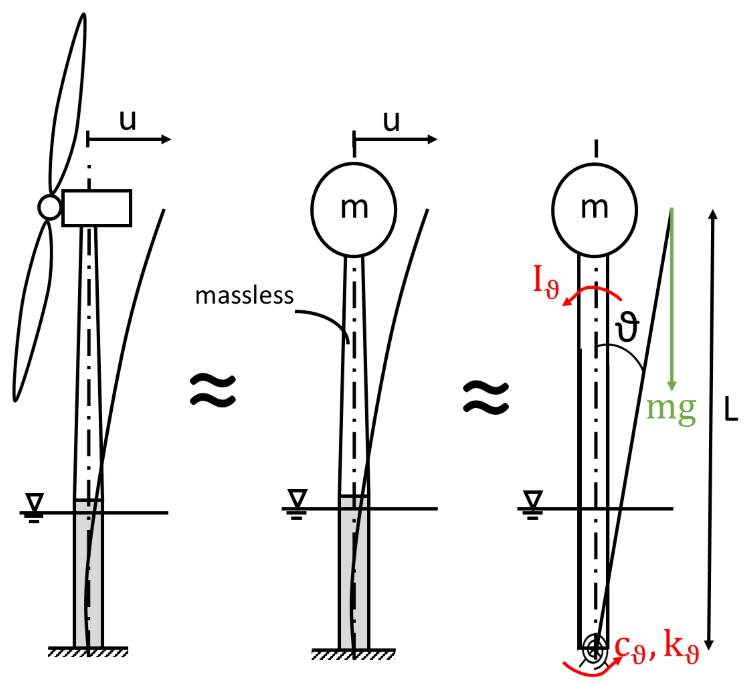
A simplified monopile, modeled as an inverted pendulum, is used to assess the applicability of the domain decomposition in deriving response statistics in non-Gaussian seas. This equivalent monopile is modeled through the capabilities already existing in OpenFOAM’s rigid body motion solver, which is frequently used for floating structures. As illustrated in Figure 2, the monopile is gradually simplified to a rigid inverted pendulum with a spring-damper hinge connection at the bottom of the wave flume, which adequately emulates the original monopile-tower assembly first fore-aft bending mode. Although doing so implies that the motion of the structure in the water is overestimated due to stiff modeling of the pile, this should give a first idea considering the possible impact of random wave loading on monopiles.
First, the monopile is reduced to a one degree-of-freedom system, for which the free vibration has been written down in Equation (6).
In Equation (6), m is the sum of the lumped mass of the tower and monopile assembly and the mass of the rotor and hub, c is the viscous damping based on the modal damping factor, , of 0.01 and k in this context the stiffness derived for the cantilevered beam.
Assuming the tower-monopile assembly to be stiff and massless, the equation of motion for the first fore-aft bending mode in Equation (6) then reduced to the momentum equilibrium, in terms of , for an inverted pendulum freely rotating about a spring-damper hinge, as illustrated in the free body diagram on the right-hand side of Figure 2.
In Equation (7), signifies the inertia about the spring-damper hinge, L the length of the tower-monopile assembly and g the gravitational constant. Enforcing the natural frequency and the modal damping, the equivalent spring-damper hinge constants and can be readily derived. As can be clearly noted, it has to be borne in mind that contrary to the original structural bending model with its inherent small angle approximations, the pendulum model in OpenFOAM takes into account the second-order effect associated with gravity. Hence, the moment resulting from gravity has to be taken along when determining the spring hinge stiffness, .
In Equation (8), the full expression for the momentum equilibrium of the equivalent monopile in water is shown, with a the added mass, the hydrodynamic damping, the hydrodynamic restoring coefficient and M the moment resulting from the hydrodynamic forcing.
As such, the monopile is reduced to a one-degree-of-freedom rigid body system with appropriate restraints and structural parameters. Its hydrodynamic properties are implicitly taken along by adopting several loops over the fluid solver and the rigid body motion solver.
3. Numerical Set-Up
3.1. Far Field
As a far field domain, a numerical wave basin of 25 peak wavelengths and 40 m water depth is modeled in HOS-NWT at full-scale, nihilating any possible scale effects, which should be sufficient for the considered sea state to develop its nonlinear characteristics. However, instead of the deep water waves considered in Toffoli et al. [12], intermediate conditions are studied here, which reduces the wave growth rate. An equilibrium state regarding non-Gaussianity might therefore not be reached by the end of the wave basin. At the inlet of the basin, waves are generated by a numerical flap-type wave maker from a JONSWAP spectrum applying linear wave maker theory. Input parameters to the wave maker are peak enhancement factors, , of 1, 3.3 and 6, a steepness, , of 0.1 and a relative water depth, , equal to 2, i.e., a moderately steep sea state in intermediate water depth, which corresponds to an environment where a monopile would be typically built. depicts the peak wave number and the significant wave height. A grid of 512 × 1 × 128 points, i.e., a spatial resolution of 11.29 m and a maximum resolvable frequency of 0.372 Hz, is used, which provides about ten points to model the peak wave length and two points for the smallest wave length. Wave data are sampled at 50 Hz. Furthermore, the HOS solutions are truncated at third order of nonlinearity, allowing for the nonlinear wave–wave interactions to occur [12]. Wave gauges are equidistantly placed along the full length of the wave flume at an interval of one peak wavelength. To prevent wave reflection at the end of the basin, a numerical relaxation zone of two peak wavelengths is provided at the outlet of the basin.
For each peak enhancement factor, seven runs of 1000 s were run, which amounts to approximately 7000 waves per input spectrum. One serial run for the far field model takes a CPU time of about 12 h for three hours of wave data on one Intel Xeon CPU E5-2630 v3 at 2.40 GHz × 16.
3.2. Near Field
3.2.1. Numerical Wave Flume
For the near field model, the latest version of the wave generation and absorption toolbox olaFlow is used together with OpenFOAM-v1906+. The near field is represented by a wave flume of total length five peak wavelenghts with the monopile being located at two peak wavelengths from the inlet. A schematic view of the near field domain is shown in Figure 3.
The waves obtained from HOS-NWT at two wavelengths before the location of interest are, after filtering, are input to olaFlow’s irregular wave generation boundary. To reconstruct the exact same time series and retain the non-Gaussianity developed over the course of the HOS-NWT model, the original phases are input to the irregular wave generation as well. In doing so, the result of the nonlinear wave–wave interactions developed up to the equivalent position of the near field wave generation boundary in the far field is retained. The remaining interactions to occur in between the wave generation boundary and the monopile are then taken care of by the near field CFD model. The benchmark will provide more insight in the validity of these assumptions and the near field resolution needed to guarantee correct reproduction of the original time-series.
At the outlet, active (shallow water) wave absorption is applied. As mentioned before, although olaFlow makes for fast evaluation of wave absorption profiles, it is meant to actively compensate shallow water velocity profiles [28]. Therefore, the (exponential) velocity profiles associated with deeper water waves cannot be adequately absorbed. In Higuera [29], several options for improvement to olaFlow’s active wave absorption, i.e., by slightly reformulating the original compensating velocity field and by combining it with passive wave absorption, are explored, generally arriving at reduced reflection at higher computational cost. Instead of applying these proposed improvements, acceptable and computationally efficient wave absorption will be obtained by including a domain of two peak wavelengths consisting of cells of increasing dimensions towards the active wave absorbing boundary, taking full advantage of numerical dissipation. Further on in this work, a reflection analysis along the lines Mansard and Funke [30] will assess the validity of this approach.
In benchmarking the hybrid HOS-CFD approach, the near-field numerical wave flume is modeled as two-dimensional. One run for the herein presented near field 2-D CFD model takes about 72 h on one Intel Xeon CPU E5-2630 v3 at 2.40 GHz × 16 for 3600 s.
3.2.2. Structural Model
As input to the structural model, the monopile presented by Jonkman and Musial [31] with the 77.6 m high National Renewable Energy Laboratory (NREL) 5 MW reference wind turbine by Jonkman et al. [32] on top is used. For nonlinear wave–wave interactions to occur, must be valid [7]. Therefore, an intermediate water depth of 40 m was chosen and the original monopile of 30 m length in a water depth of 20 m is lengthened up to 50 m. The monopile diameter of 6m and wall thickness of 0.06 m are kept the same. As mentioned earlier, the equivalent monopile is modeled by using OpenFOAM’s rigid body motion solver applying appropriate translational restraints and a spring-damper hinge constraint. The mass at the tower top is taken to be the sum of the actual mass of the rotor-hub-nacelle assembly and the lumped tower-monopile mass under the assumption of a clamped connection at the sea floor. The moment of inertia is then simply determined as this mass times total height squared. Knowing the dry natural frequency and the modql damping ratio, the stiffness and damping coefficients can then be readily derived. The original monopile properties and the equivalent monopile input to the structural model are listed in Table 1.
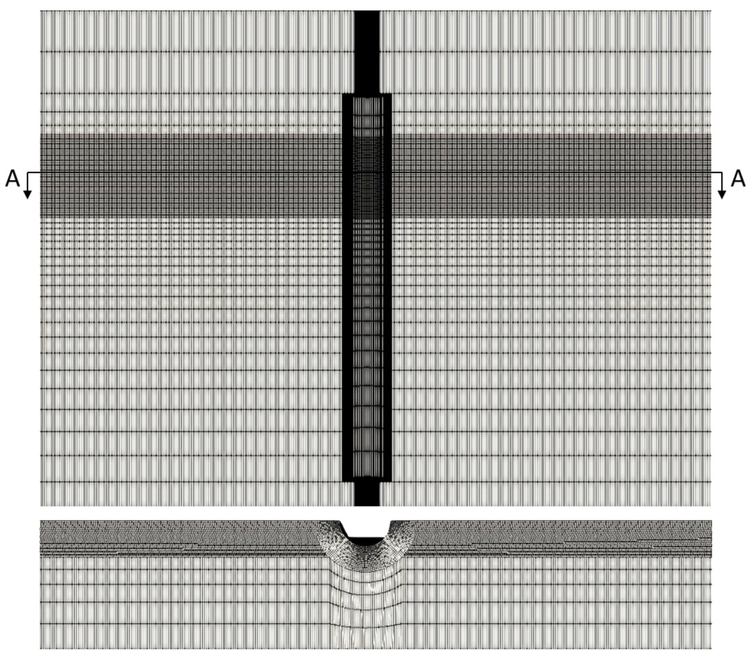
For the structural computations, the numerical wave flume is modeled by expanding the near field domain in Figure 3 up to 3D and by including the equivalent monopile model presented in Figure 2. As , with D the structural diameter, viscosity is not negligible, but as the Keulegan-Carpenter (KC) number corresponding to the peak of the input spectrum is still small () no vortex shedding is to be expected. Taking into account the absence of asymmetric vortex shedding and the structural symmetry, it is appropriate to model only half of the domain and the structure, applying symmetry boundary conditions at the symmetry surface, and thus saving considerate computational resources. The resulting three-dimensional mesh is shown in Figure 4. As can be seen in Figure 4, throughout the mesh in the x-direction the target refinement is withheld. For the y- and z-direction, gradual refinement is adopted towards this target refinement in the vicinity of the monopile and the wave surface. As part of the benchmark, this target refinement about the monopile and the free surface will be varied.
Simulations are run with an adaptive time step defined by a maximum Courant number (Co) of 0.5. Furthermore, OpenFOAM’s interFoam solver adopts the two inner loops for the pressure correction typically of PISO and three outer PIMPLE loop iterations to force convergence between the rigid body and the spring-damper hinge on the one hand and the wave–structure interaction on the other hand during each time step. As the motion in the water is limited, this small number of outer loops suffices. Relaxation and damping factors of, respectively, 0.95 and 0.90 are enforced in the rigid body solver using the implicit second-order Crank–Nicolson scheme. The terms in the Navier–Stokes are discretized using Gaussian integration and using Euler explicit time stepping. Preconditioned conjugate gradient and stabilized bi-conjugate gradient solvers are used for respectively solving for the initial guess for the velocities and the pressure correction equation.
Waves are presented to the near field’s numerical wave basin. Both the surface elevation and the structural response are sampled at 50 Hz. For each wave case seven realizations were fed to the near field and run for three weeks on five Intel Xeon CPU’s E5-2680 v2 at 2.8 GHz × 20, resulting in time series of approximately 1000 s, i.e., 160 peak waves. The actual length of the obtained time series depended on the spectra simulated, because the irregular wave surface associated with broad-bandedness gives rise to more spurious air velocities at the air-water surface, which significantly reduced the adaptive time steps. Simulating for the Pierson–Moskovitz spectrum took longer than the narrow-banded JONSWAP spectrum generally.
4. Results
4.1. Benchmark for the Wave Field
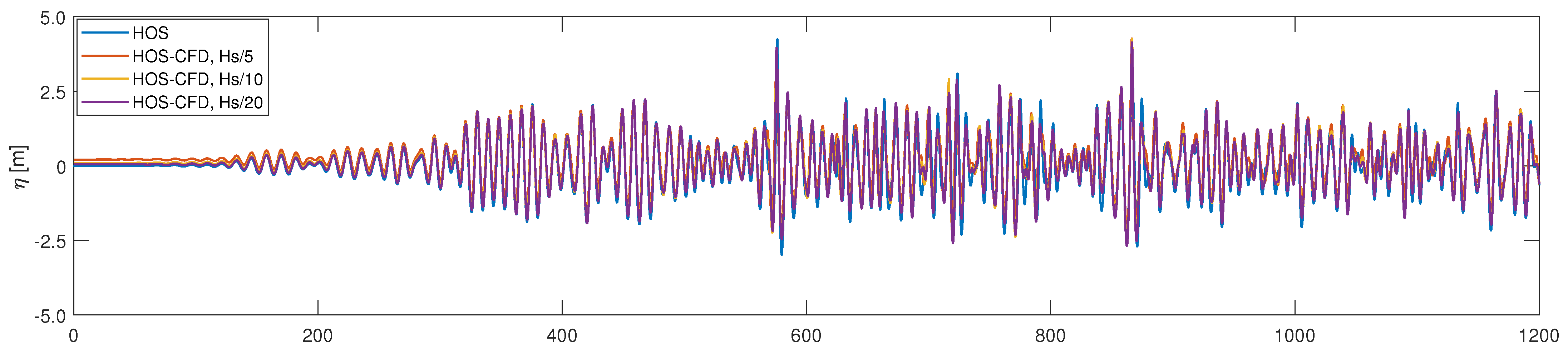
Before running the fully coupled HOS-CFD model, a benchmark study was conducted to verify the validity of the proposed domain decomposition strategy regarding the wave fields involved and to identify probable discrepancies between the HOS solution and the coupled HOS-CFD solution and their causes. In doing so, first, the HOS model has been used to compute the wave series at 23 peak wavelengths from the models’ wave maker. Next, the time series obtained two peak wavelengths back, was applied to the near field boundary and the CFD model was used to let the wave further evolve. Finally, the time series logged at the location of the would-be structure in the CFD model was compared to the original time series obtained at that very same position in the HOS model. The result is presented in Figure 5 for three different near field mesh resolutions, i.e., Hs/5, Hs/10 and Hs/20.
From Figure 5, it can be clearly seen that the signals of the coupled HOS-CFD and of HOS-NWT correspond closely both in terms of phases and peaks for all considered mesh resolutions. As mesh resolution increases, the reconstructed signal in HOS-CFD converges to the target signal obtained from HOS-NWT. Good agreement is found for Hs/20, although the signal corresponding to a resolution Hs/10 is a very close second. As optimal reconstruction of the target signal is key in this work, Hs/20 will be withheld in further considerations. Occasionally, slight underestimations are observed for the waves compared to their HOS counterparts. These underestimations are rather small at the beginning of the time series, but grow more pronounced towards the end. Two explanations for these observed differences in peak values seem plausible.
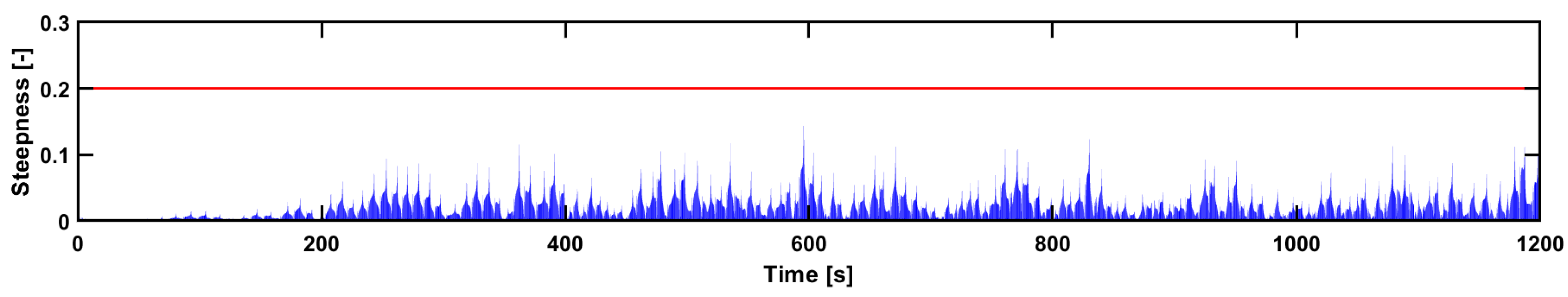
Firstly, no breaking model is included in HOS-NWT, while waves in OpenFOAM might prematurely break, i.e., before reaching their breaking limit, or lose energy to dissipation. Although publicly available HOS-NWT does not incorporate breaking models and dissipation, it does include a limit to the steepness above which the computation breaks down. Still, large peaks that overshoot the physics might be encountered. On the contrary, OpenFOAM’s interFoam solver does include viscosity and two-phase fluid interaction through diffusive transport equations for cell water fractions. The evolution of wave fields can therefore be expected to be more realistic in the sense that they are allowed to break. However, due to the dissipative nature of these transport equations, waves might lose energy to numerical dissipation. Therefore, a breaking detection was performed on the HOS output signal for with a the wave amplitude, the wave frequency and the wave limiting steepness. As this condition is only applicable for linear waves, the assessment of the wave breaking is based on a characteristic wave amplitude and characteristic wave frequency computed for each time instance by applying wavelet analysis along the lines of Liu and Babanin [33] with a limiting value, , of 0.2. As can be seen from Figure 6, the considered wave field from HOS is in no danger of breaking.
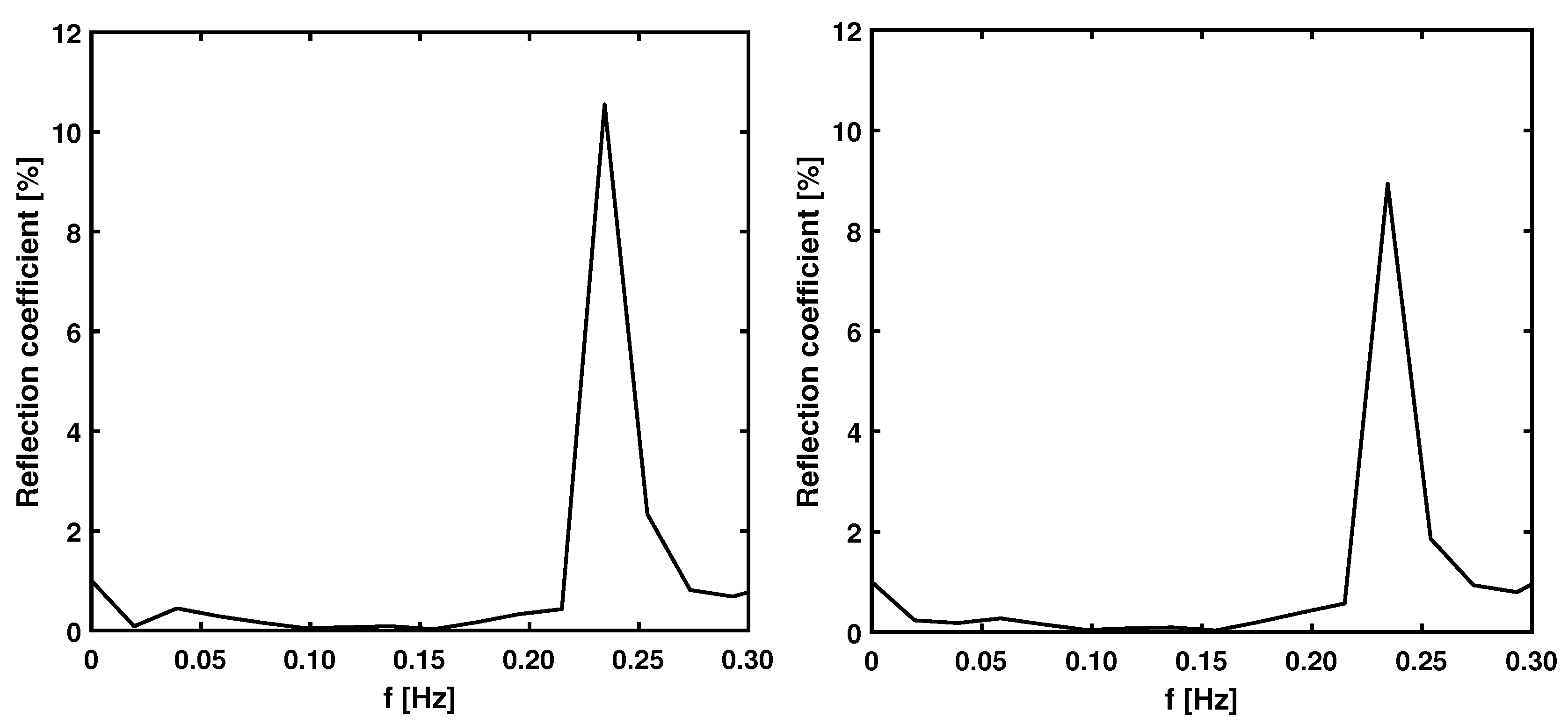
On the other hand, the differences in peak values could be attributed to the different wave absorption strategies used in HOS-NWT and the CFD model; in HOS-NWT a passive absorption based on numerical relaxation is applied, while in olaFlow active (shallow water) absorption combined with additional numerical dissipation is adopted. Therefore, a reflection analysis according to Mansard and Funke [30], has been applied to both HOS-NWT and CFD at the same respective positions. When comparing the reflection coefficients in Figure 7, it is clear that HOS-NWT shows larger reflection at the high frequencies.
Notwithstanding, the known inaccuracies of the reflection analysis with respect to the high-frequency tail, about 9% reflection can be noted in the high-frequency tail for CFD, while approximately 11% reflection is shown for HOS-NWT. Both models display small values for the reflection coefficient in the low-frequency tail as well. The values for the reflection coefficient for the HOS-NWT model are generally higher than the ones for the CFD model. This difference in absorbing long waves can be explained by the inherent differences between the active and passive wave absorption applied. As olaFlow is aimed at absorbing shallow water waves, it simply absorbs long waves best. Furthermore, in HOS-NWT, a numerical relaxation zone of two peak wavelengths is used, resulting in the increased reflection of wave components slightly longer than this zone.
The waves obtained by both the CFD and the coupled HOS-CFD model collide remarkably well. Discrepancies can most certainly be attributed to the differences in absorption strategy.
4.2. Verification of the Equivalent Monopile
In order to verify the applied simplified inverted pendulum model and to improve the understanding of the wave–structure interaction results further on, a free decay test for the model’s pitch motion has been conducted in the numerical wave flume. Figure 8 shows the pitch motion, , as it decays in time. Applying modal analysis through the MATLAB toolbox MACEC 3.3 [34], the natural frequency and the damping ratio are defined as respectively 0.253Hz and 1.4%, which lies close to the target values earlier defined in Table 1.
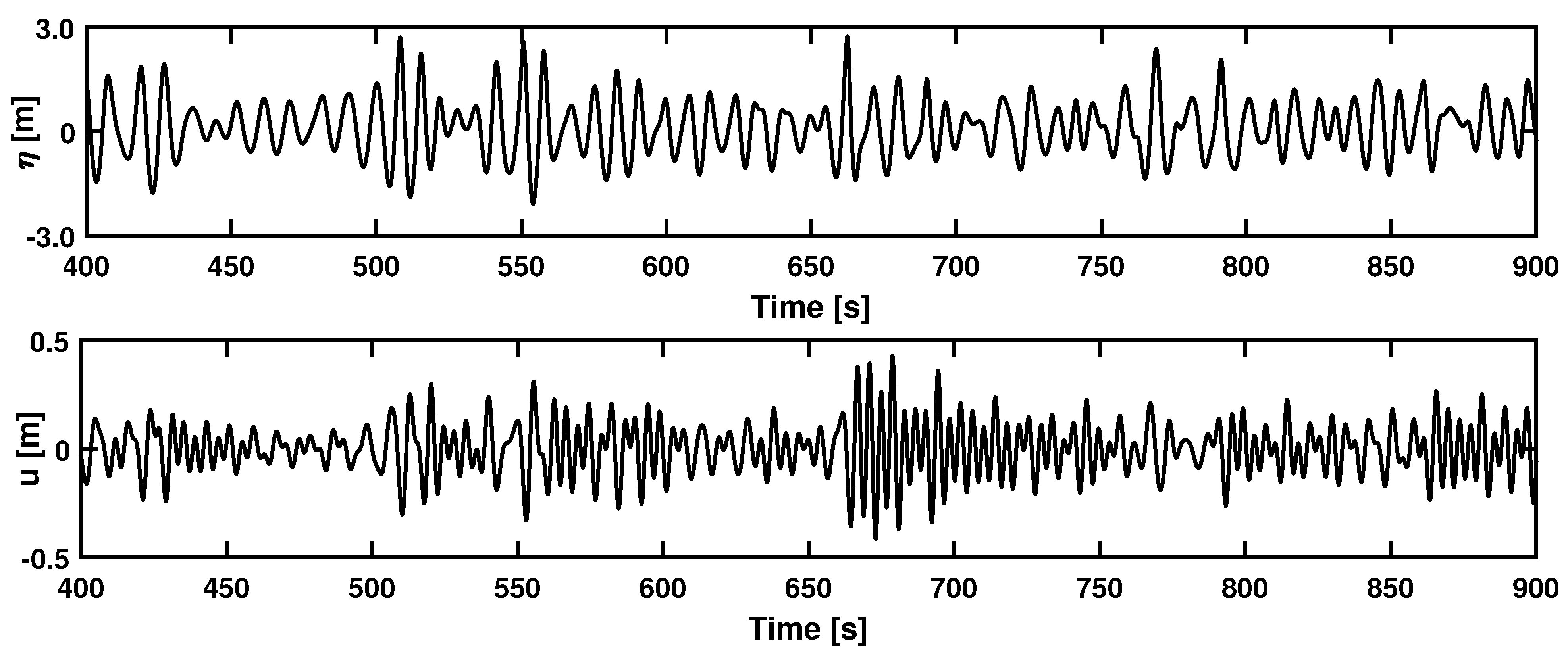
Furthermore, as can be seen from Figure 9, the equivalent monopile response closely mimics the wave elevation, which is expected as the natural frequency is situated on the right-hand side of the wave peak frequency. The high-frequency stiff monopile response is superposed onto the quasi-static response to the waves. Even for the short window presented, multiple high-frequency events can be noted. The most notable one is situated in between 650 and 700 s and corresponds most plausibly to a typical high-frequency ringing event; the response appears to build up over several periods and subsequently decays.
The equivalent monopile is therefore not only able to reproduce the monopile’s structural properties, it captures its typical high-frequency behavior as well. Having verified the validity of both the domain decomposition and the equivalent monopile, in the remainder of this work, some statistics regarding the waves and the responses will be drawn and their reliability will be assessed.
4.3. Application to Obtaining Non-Gaussian Response Statistics
While adopting the same wave parameters as previously used for the benchmark study, the applicability of the proposed domain decomposition strategy to obtaining response statistics for structures in non-Gaussian seas is hereafter studied. Seven Monte Carlo realizations of about 500 peak waves have been simulated for three wave spectra with different peak wave factors; i.e., 1, 3.3 and 6. The input spectra were chosen to contain similar energy content, i.e., same zero-order moment, , or standard deviation, . Using different spectral peak factors changes the shape of the wave spectrum with the spectrum corresponding to classified as broad-banded and the one with being narrow-banded.
Narrow-banded spectra are known to be especially prone to a special case of resonant wave–wave interactions, the so-called Benjamin–Feir instability, which modulates a wave train originally narrow-banded by exchanging energy with its close side-bands. As the Benjamin–Feir instability modulates narrow-banded wave trains, it is a considered to be a plausible candidate in explaining the formation of freak waves [35]. The Benjamin–Feir instability manifests itself to differing degrees in long-crested deep to intermediate water wave trains () [7,23]. Onorato et al. [36] summarized the influence of bandwidth and water depth on the occurrence of the Benjamin–Feir instability in the Benjamin–Feir index (BFI) as
with factors and for finite water depths defined as
The Benjamin–Feir indices for the herein considered wave spectra then become 0.09, 0.58 and 0.73 for respectively , the highest BFI incorporating the fact that instabilities will most likely occur for narrow-banded spectra.
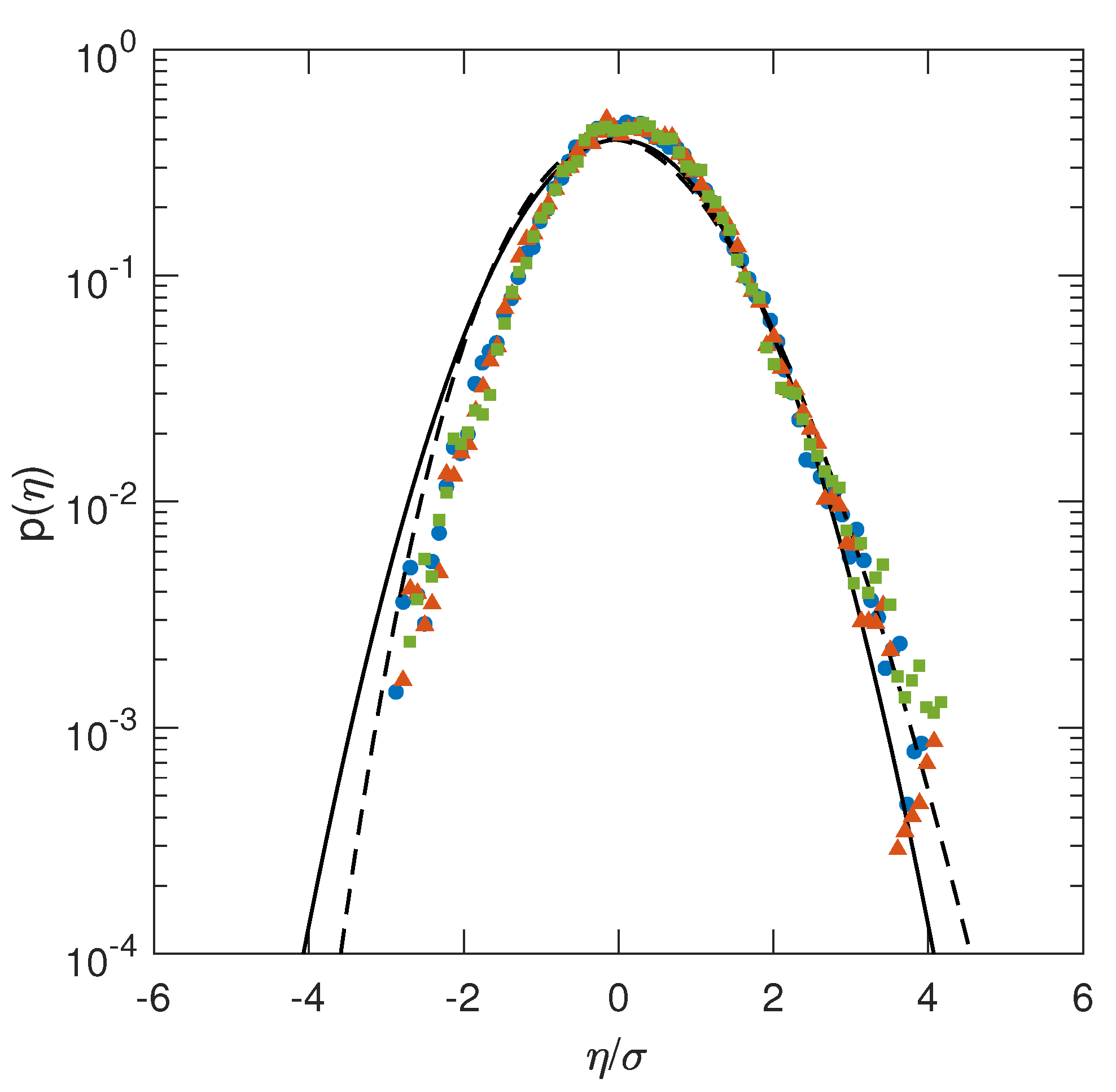
Figure 10 shows the probabilities of the wave elevations captured in the near field for the three wave spectra considered. These wave elevations correspond to the sea state captured at 23 peak wavelengths from the wave maker in the far field. For the sake of comparison, all wave elevations are normalized by their standard deviation . In addition, the normal probability density function and its second-order correction, computed along the lines of Tayfun [37], are shown. From Figure 10, all realizations appear to be skewed with respect to the Gaussian. The positive surface elevations evidently conform closest to the Tayfun distribution. However, the negative values overestimate the values expected for typically second-order waves. Furthermore, not much can be said regarding the differences between the spectra.
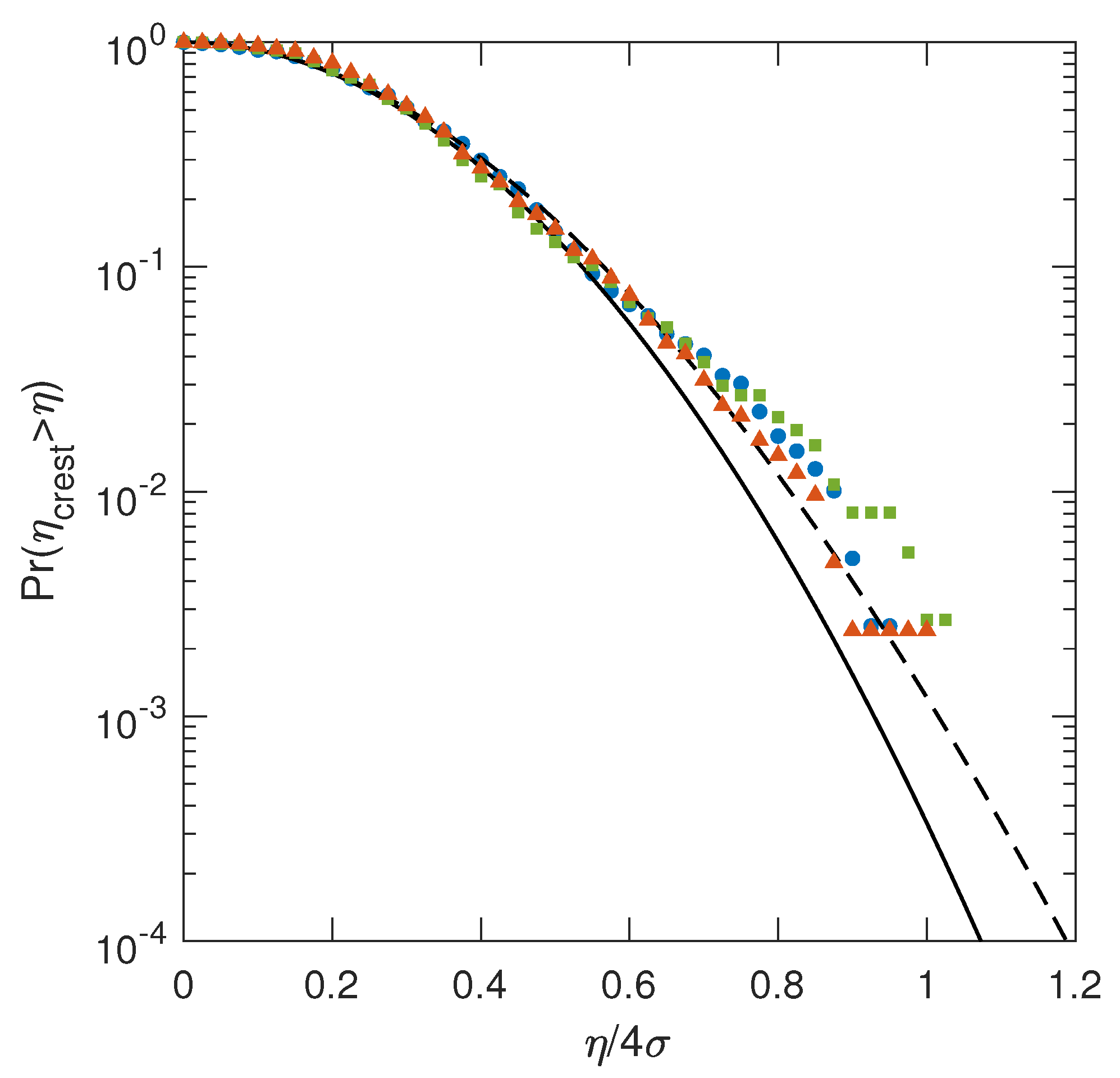
In Figure 11, the probability distributions for the wave crests are shown. The thresholds have been normalized by their wave height, i.e., . For comparison, the Rayleigh distribution, to which wave crests for linear waves tend, are drawn together with the Tayfun distribution for second-order wave crests. As expected, the wave crests resulting from all three wave specra conform best to the Tayfun distribution. Depending on the bandedness of the spectra, differences in wave crest distribution can be noted as well. For the largest BFI, corresponding to the narrow-banded case, strongest deviations from the Tayfun distribution can be noted. Overall, the statistics presented in Figure 11 are in strong agreement with the works by Onorato et al. [36] and Toffoli et al. [7].
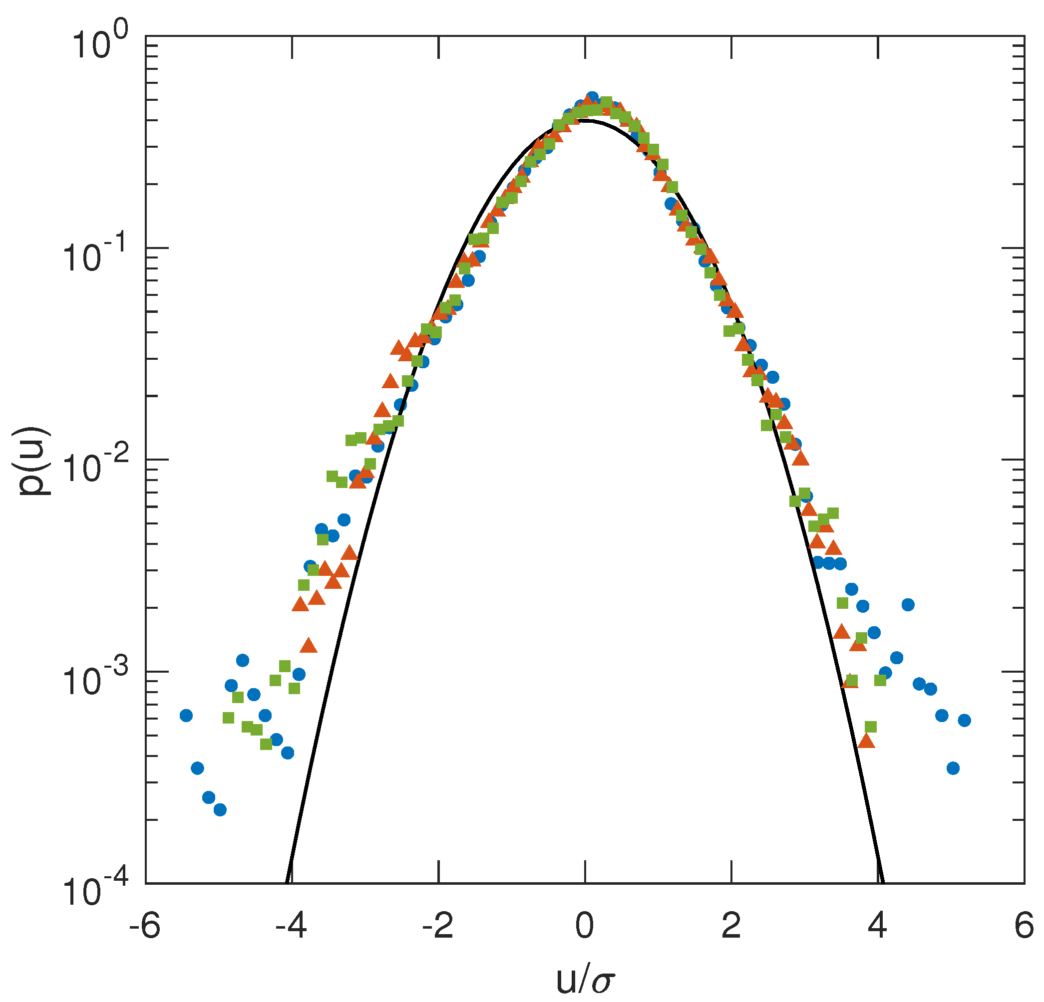
Figure 12 shows the tower top excursions with respect to the Gaussian. All displacements have been normalized by their respective standard deviation. The skewness of the responses compared to the Gaussian appears to reflect the skewness originally found for the probability density function of the wave elevations in Figure 10. Compared to Figure 10, the lower and upper tails seem to be heavier and clear differences are noted depending on wave spectral bandedness. The tails seem to be heaviest for the broad-banded specrum, corresponding to lowest BFI, while the narrow-banded wave spectrum results in slightly heavier tails than does the response spectrum corresponding to .
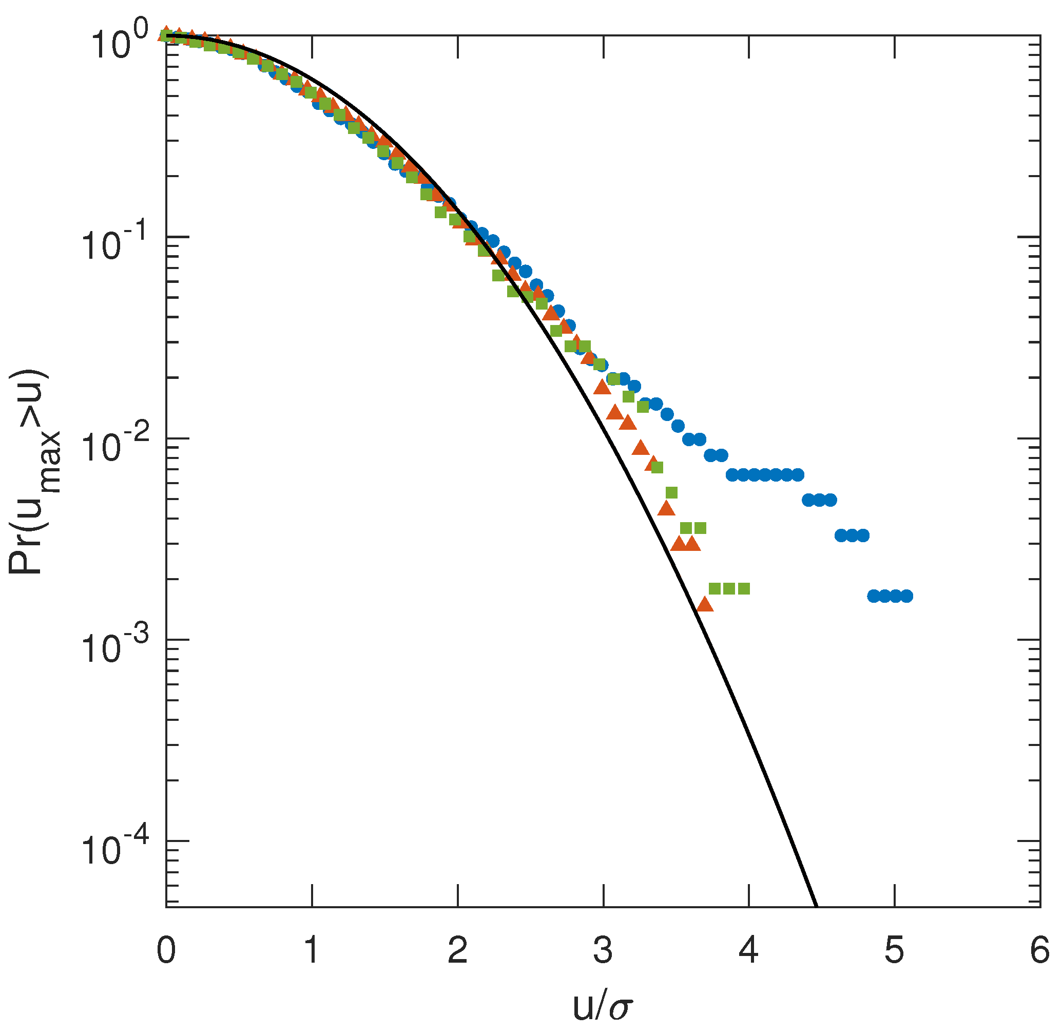
Moreover, Figure 13, depicting the probability distribution for the tower top displacements, appears to confirm the more extreme responses already found in the upper tail in Figure 12 for the broad-banded spectrum. Similarly, the narrow-banded spectrum results in more extreme responses than does the wave spectrum lying in between.
The largest response noted for the broad-banded spectrum could be attributed to its heavier high-frequency spectral tail, which continuously excites the tower’s first fore-aft bending resonant frequency. The remaining narrower-banded wave spectra have similar energy in their tails, with the narrowest-banded wave spectrum having obviously the least. Interestingly though, the narrowest-banded wave spectrum results in larger response than does the wave spectrum corresponding to . Therefore, energy considerations probably not tell the full story.
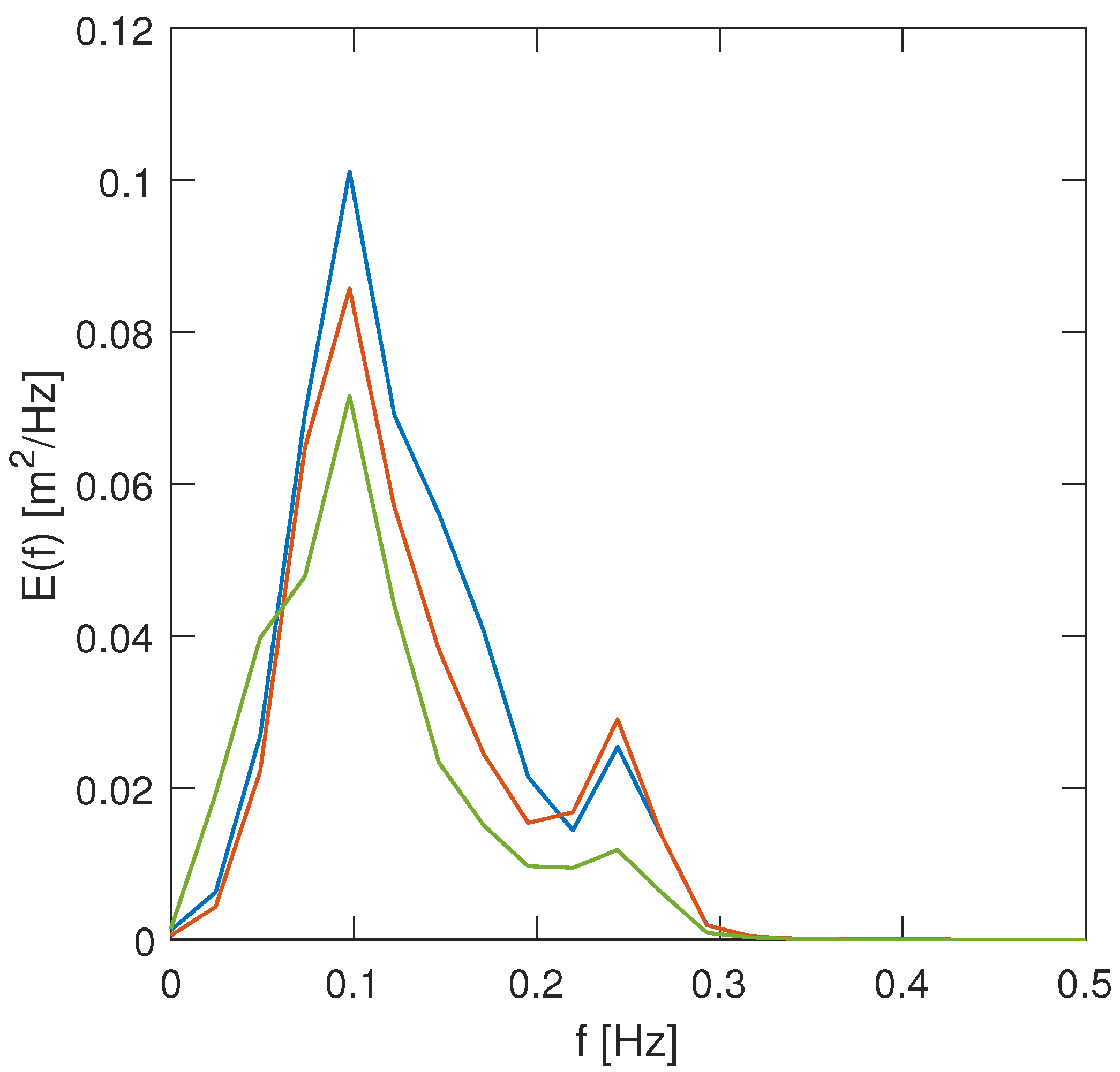
Figure 14, depicting the response spectra for the considered wave spectra smoothed using a Hann window of 512 samples (sampled at 50 Hz) and averaged over the seven realizations, shows that indeed the broad-banded wave spectrum results in highest response in its tail. The second broadest wave spectrum appears to do so as well. The narrow-banded spectrum shows overall the least energy. Therefore, it is most plausible that the larger response for the narrowest-banded spectrum as noted in Figure 13 originates from the larger waves associated with the higher probability of occurrence of the Benjamin–Feir instability. Moreover, looking at the response spectra, one would expect the response at the wave spectral peak to be largest for the narrow-banded wave spectrum and smallest for the broad-banded wave spectrum.
5. Discussion
From the above presented results, the proposed domain decomposition strategy is clearly able to both reproduce the non-Gaussianity of the wave field obtained from HOS-NWT with remarkable accuracy and capture some interesting dynamic response phenomena. Furthermore, a link appears to exist between the non-Gaussian wave statistics obtained through the decomposed model and the perceived simplified monopile responses, indicating that the model could be applied to studying the impact of nonlinear wave–wave interactions in offshore structural response. During this study, the question was raised of whether such a model would be able to generate enough data for converged response statistics. In answering this question, three points have to be considered: the extent of the data gathered and the sampling rate; the availability of computational resources; and most importantly, the response characteristics of the structure under consideration.
Regarding the first point, reducing the sampling frequency by five could deliver data at one-third of the above-mentioned computational costs as a large overhead exists in CFD in writing data to disk space, still leaving us at 7 × 1 week of computational time on five Intel Xeon CPU’s E5-2680 v2 at 2.8 GHz × 20. per wave spectral case. Having sufficient computational resources, simulating for two months would deliver enough data, i.e., ±10,000 waves, for a simple stiff structures as is the monopile. This is in line with the amount of waves previously used in studying modulational instability as one of the mechanisms underlying extreme wave formation [7].
For the monopile, the results indicate that nonlinear wave–wave interactions have their influence on its response statistics. Obviously, the Pierson–Moskowitz spectrum continuously excites the first fore-aft bending natural frequency due to its relatively high energy content in its high-frequency tail. However, results also indicate that although its limited energy content in the upper spectral tail, narrow-banded wave spectra might lead to larger response maxima than does a traditional JONSWAP spectrum characterized by . Based on the premise that narrow-banded waves lead to a higher occurrence of extreme waves and taking into account the ringing observed in Figure 9, a plausible guess could be that ringing more often occurs for these narrow-banded spectra. The above presented results agree with what would be expected from literature and therefore confirm the applicability of the proposed model in studying response statistics in non-Gaussian seas. Nonetheless, it has to be borne in mind that these preliminary observations are based on statistics that are not converged yet.
When considering compliant floating structures, eigenfrequencies are about an order of magnitude lower than, e.g., the monopile’s first natural frequency. Many more data would therefore be needed to arrive at converged response statistics for compliant structures. The bottleneck lies in the number of realizations of the slow difference frequency response realizations rather than the amount of waves. Computations are expected to become truly demanding in cases of 3D motion and directional wave fields, rendering the previously applied symmetry plane invalid. Therefore, although the model has shown to be able to capture the response phenomena related to nonlinear wave–wave interactions in non-Gaussian seas, and the estimate of the cost required for converged results for stiff offshore structures seems reasonable, the proposed methodology is not expected to be feasible for 3D motion, directional wave fields and compliant structures.
6. Conclusions
In this work, a time-domain approach for the response statistics in non-Gaussian seas based on domain decomposition through coupling between HOS-NWT and OpenFOAM has been proposed to overcome the combined cost of detailled near field CFD and the long domains needed for waves to develop the required non-Gaussian properties. A benchmark case for the coupled HOS-CFD model showed that the peaks and phases of the wave signal obtained by HOS-NWT are well reproduced. Furthermore, an equivalence between the monopile and its simplified structural model adopted herein exists, which allows one to capture typical hydrodynamic phenomena, such as ringing. It appears to be possible to deduce response statistics regarding the impacts of nonlinear wave–wave interactions, and a major implication for further research was found, as the wave extremes for the narrow-banded spectrum were mirrored in the corresponding response. However, not enough data were obtained for these observations to be conclusive.
Due to computational cost, the proposed methodology seems to be limited to stiff structures and unidirectional wave trains.
Author Contributions
Conceptualization, G.D. and A.T.; methodology, G.D. and A.T.; software, G.D.; validation, G.D..; formal analysis, G.D.; investigation, G.D.; resources, J.M. and A.T.; data curation, G.D.; writing—original draft preparation, G.D.; writing—review and editing, G.D., A.T., J.M and G.L.; visualization, G.D.; supervision, A.T., J.M. and G.L.; project administration, J.M. and G.L.; funding acquisition, G.D. and J.M. All authors have read and agreed to the published version of the manuscript.
Funding
This research was funded by the Research Foundation—Flanders grant numbers 11A1217N and V431019N.
Acknowledgments
The first author is a Ph.D. fellow of the Research Foundation—Flanders (FWO) (Ph.D. fellowship 11A1217N). This specific collaborative research came to fruition thanks to the travel grant awarded to the first author (Long stay travel grant V31019N) by the Research Foundation—Flanders (FWO).
Conflicts of Interest
The authors declare no conflict of interest.
References
- Breton, S.P.; Moe, G. Status, plans and technologies for offshore wind turbines in Europe and North America. Renew. Energy 2009, 34, 646–654. [Google Scholar] [CrossRef]
- Bilgili, M.; Yasar, A.; Simsek, E. Offshore wind power development in Europe and its comparison with onshore counterpart. Renew. Sustain. Energy Rev. 2011, 15, 905–915. [Google Scholar] [CrossRef]
- Bhattacharya, S. Challenges in design of foundations for offshore wind turbines. Eng. Technol. Ref. 2014, 1, 922. [Google Scholar] [CrossRef]
- DNV GL. DNV-OS-J103—Design of Floating Wind Turbine Structures. Available online: https://rules.dnvgl.com/docs/pdf/DNV/codes/docs/2013-06/OS-J103.pdf (accessed on 6 January 2021).
- Moan, T.; Zheng, X.Y.; Quek, S.T. Frequency-domain analysis of non-linear wave effects on offshore platform responses. Int. J. Non-Linear Mech. 2007, 42, 555–565. [Google Scholar] [CrossRef]
- Onorato, M.; Osborne, A.R.; Serio, M.; Cavaleri, L.; Brandini, C.; Stansberg, C. Extreme waves, modulational instability and second order theory: Wave flume experiments on irregular waves. Eur. J. Mech. B/Fluids 2006, 25, 586–601. [Google Scholar] [CrossRef]
- Toffoli, A.; Onorato, M.; Bitner-Gregersen, E.; Osborne, A.R.; Babanin, A. Surface gravity waves from direct numerical simulations of the Euler equations: A comparison with second-order theory. Ocean Eng. 2008, 35, 367–379. [Google Scholar] [CrossRef]
- Schløer, S.; Bredmose, H.; Bingham, H.B. The influence of fully nonlinear wave forces on aero-hydro-elastic calculations of monopile wind turbines. Mar. Struct. 2016, 50, 162–188. [Google Scholar] [CrossRef]
- Engsig-Karup, A.P.; Bingham, H.B.; Lindberg, O. An efficient flexible-order model for 3D nonlinear water waves. J. Comput. Phys. 2009, 228, 2100–2118. [Google Scholar] [CrossRef]
- Dommermuth, D.G.; Yue, D.K. A high-order spectral method for the study of nonlinear gravity waves. J. Fluid Mech. 1987, 184, 267–288. [Google Scholar] [CrossRef]
- West, B.J.; Brueckner, K.A.; Janda, R.S.; Milder, D.M.; Milton, R.L. A new numerical method for surface hydrodynamics. J. Geophys. Res. Ocean. 1987, 92, 11803–11824. [Google Scholar] [CrossRef]
- Toffoli, A.; Gramstad, O.; Trulsen, K.; Monbaliu, J.; Bitner-Gregersen, E.; Onorato, M. Evolution of weakly nonlinear random directional waves: Laboratory experiments and numerical simulations. J. Fluid Mech. 2010, 664, 313–336. [Google Scholar] [CrossRef]
- Weller, H.G.; Tabor, G.; Jasak, H.; Fureby, C. A tensorial approach to computational continuum mechanics using object-oriented techniques. Comput. Phys. 1998, 12, 620–631. [Google Scholar] [CrossRef]
- Paulsen, B.T.; Bredmose, H.; Bingham, H.B. An efficient domain decomposition strategy for wave loads on surface piercing circular cylinders. Coast. Eng. 2014, 86, 57–76. [Google Scholar] [CrossRef]
- Paulsen, B.T.; Bredmose, H.; Bingham, H.B.; Jacobsen, N.G. Forcing of a bottom-mounted circular cylinder by steep regular water waves at finite depth. J. Fluid Mech. 2014, 755, 1–34. [Google Scholar] [CrossRef]
- Jacobsen, N.G.; Fuhrman, D.R.; Fredsøe, J. A wave generation toolbox for the open-source CFD library: OpenFoam®. Int. J. Numer. Methods Fluids 2012, 70, 1073–1088. [Google Scholar] [CrossRef]
- Alberello, A.; Pakodzi, C.; Nelli, F.; Bitner-Gregersen, E.M.; Toffoli, A. Three dimensional velocity field underneath a breaking rogue wave. In Proceedings of the ASME 2017 36th International Conference on Ocean, Offshore and Arctic Engineering, Trondheim, Norway, 25–30 June 2017. [Google Scholar]
- Di Paolo, B.; Lara, J.L.; Barajas, G.; Losada, Í.J. Wave and structure interaction using multi-domain couplings for Navier-Stokes solvers in OpenFOAM®. Part I: Implementation and validation. Coast. Eng. 2020, 103799. [Google Scholar] [CrossRef]
- Larsen, B.E.; Fuhrman, D.R.; Roenby, J. Performance of interFoam on the simulation of progressive waves. Coast. Eng. J. 2019, 61, 380–400. [Google Scholar] [CrossRef] [Green Version]
- Luquet, R.; Ducrozet, G.; Gentaz, L.; Ferrant, P.; Alessandrini, B. Applications of the SWENSE Method to seakeeping simulations in irregular waves. In Proceedings of the 9th International Conference on Numerical Ship Hydrodynamics, Ann Arbor, MI, USA, 5–8 August 2007. [Google Scholar]
- Gatin, I.; Vukčević, V.; Jasak, H. A framework for efficient irregular wave simulations using Higher Order Spectral method coupled with viscous two phase model. J. Ocean Eng. Sci. 2017, 2, 253–267. [Google Scholar] [CrossRef]
- Gatin, I.; Vladimir, N.; Malenica, Š.; Jasak, H. Green sea loads in irregular waves with Finite Volume method. Ocean Eng. 2019, 171, 554–564. [Google Scholar] [CrossRef]
- Toffoli, A.; Benoit, M.; Onorato, M.; Bitner-Gregersen, E. The effect of third-order nonlinearity on statistical properties of random directional waves in finite depth. Nonlinear Process. Geophys. 2009, 16, 131. [Google Scholar] [CrossRef]
- Weller, Henry G and Tabor, Gavin and Jasak, Hrvoje and Fureby, Christer A tensorial approach to computational continuum mechanics using object-oriented techniques. Comput. Phys. 1998, 12, 620–631.
- Zakharov, V.E. Stability of periodic waves of finite amplitude on the surface of a deep fluid. J. Appl. Mech. Tech. Phys. 1968, 9, 190–194. [Google Scholar] [CrossRef]
- Ducrozet, G.; Bonnefoy, F.; Le Touzé, D.; Ferrant, P. A modified high-order spectral method for wavemaker modeling in a numerical wave tank. Eur. J. Mech. B/Fluids 2012, 34, 19–34. [Google Scholar] [CrossRef]
- Ducrozet, G.; Bonnefoy, F.; Perignon, Y. Applicability and limitations of highly non-linear potential flow solvers in the context of water waves. Ocean Eng. 2017, 142, 233–244. [Google Scholar] [CrossRef]
- Higuera, P.; Lara, J.L.; Losada, I.J. Realistic wave generation and active wave absorption for Navier–Stokes models: Application to OpenFOAM®. Coast. Eng. 2013, 71, 102–118. [Google Scholar] [CrossRef]
- Higuera, P. Enhancing active wave absorption in RANS models. Appl. Ocean Res. 2020, 94, 102000. [Google Scholar] [CrossRef]
- Mansard, E.; Funke, E. The Measurement of Incident and Reflected Spectra Using a Least squares Method. In Proceedings of the 17th International Conference on Coastal Engineering (ICCE), Sydney, Australia, 23–28 March 1980. [Google Scholar]
- Jonkman, J.; Musial, W. Offshore Code Comparison Collaboration (OC3) for IEA Wind Task 23 Offshore Wind Technology and Deployment; Technical Report; National Renewable Energy Lab. (NREL): Golden, CO, USA, 2010. [Google Scholar]
- Jonkman, J.; Butterfield, S.; Musial, W.; Scott, G. Definition of a 5-MW Reference Wind Turbine for Offshore System Development; Technical Report; National Renewable Energy Lab. (NREL): Golden, CO, USA, 2009. [Google Scholar]
- Liu, P.C.; Babanin, A.V. Using wavelet spectrum analysis to resolve breaking events in the wind wave time series. Ann. Geophys. 2004, 22, 3335–3345. [Google Scholar] [CrossRef]
- Reynders, E.; Schevenels, M.; De Roeck, G. MACEC 3.3: A Matlab Toolbox for Experimental and Operational Modal Analysis. 2014. Available online: https://bwk.kuleuven.be/bwm/macec/macec.pdf (accessed on 6 January 2021).
- Onorato, M.; Waseda, T.; Toffoli, A.; Cavaleri, L.; Gramstad, O.; Janssen, P.; Kinoshita, T.; Monbaliu, J.; Mori, N.; Osborne, A.R.; et al. Statistical properties of directional ocean waves: The role of the modulational instability in the formation of extreme events. Phys. Rev. Lett. 2009, 102, 114502. [Google Scholar] [CrossRef] [Green Version]
- Onorato, M.; Osborne, A.R.; Serio, M.; Cavaleri, L. Modulational instability and non-Gaussian statistics in experimental random water-wave trains. Phys. Fluids 2005, 17, 078101. [Google Scholar] [CrossRef] [Green Version]
- Tayfun, M.A. Narrow-band nonlinear sea waves. J. Geophys. Res. Ocean. 1980, 85, 1548–1552. [Google Scholar] [CrossRef]
Figure 1.
Time domain decomposition strategy.

Figure 2.
Equivalent monopile model.

Figure 3.
Schematic view of the near field time domain.

Figure 4.
Three-dimensional wave flume mesh with a simplified monopile model.

Figure 5.
Benchmark with surface elevation plotted against time for the higher-order spectral (HOS) model (blue) and the coupled model for mesh resolutions Hs/5 (red), Hs/10 (yellow) and Hs/20 (purple).
Figure 5.
Benchmark with surface elevation plotted against time for the higher-order spectral (HOS) model (blue) and the coupled model for mesh resolutions Hs/5 (red), Hs/10 (yellow) and Hs/20 (purple).

Figure 6.
Localized steepness, , plotted against time for the HOS result.

Figure 7.
Reflection coefficients for higher-order spectral numerical wave tank (HOS-NWT) (left) and OpenFOAM (right).
Figure 7.
Reflection coefficients for higher-order spectral numerical wave tank (HOS-NWT) (left) and OpenFOAM (right).

Figure 8.
Free decay test for the inverted spring-damper pendulum.

Figure 9.
Results for wave elevation (top) and structural response (bottom).

Figure 10.
Probability density function of the surface elevations with respect to the surface elevations normalized by their standard deviation, as computed by near-field time domain for BFI = 0.09 (•), BFI = 0.58 (▲) and BFI = 0.73 (■) plotted against the normal pdf (full line) and its second-order correction (dashed line).

Figure 11.
Probability distribution of the wave crests with respect to the wave elevations normalized by their standard deviations, as computed by near-field time domain for BFI = 0.09 (•), BFI = 0.58 (▲) and BFI = 0.73 (■) plotted against the Rayleigh distribution (full line) and the Tayfun distribution (dashed line).

Figure 12.
Probability density function tower top displacements with respect to the displacements normalized by their standard deviations, as computed by near-field time domain for BFI = 0.09 (•), BFI = 0.58 (▲) and BFI = 0.73 (■) plotted against the normal pdf (–).
Figure 12.
Probability density function tower top displacements with respect to the displacements normalized by their standard deviations, as computed by near-field time domain for BFI = 0.09 (•), BFI = 0.58 (▲) and BFI = 0.73 (■) plotted against the normal pdf (–).

Figure 13.
Probability distribution maximum tower top displacements with respect to the displacements normalized by their standard deviation, as computed by near-field time domain for BFI = 0.09 (•), BFI = 0.58 (▲) and BFI = 0.73 (■) plotted against the Rayleigh distribution (–).
Figure 13.
Probability distribution maximum tower top displacements with respect to the displacements normalized by their standard deviation, as computed by near-field time domain for BFI = 0.09 (•), BFI = 0.58 (▲) and BFI = 0.73 (■) plotted against the Rayleigh distribution (–).

Figure 14.
Response density spectra for the tower top displacements for (blue), (orange) and (green).
Figure 14.
Response density spectra for the tower top displacements for (blue), (orange) and (green).


Table 1.
Structural parameters for the original monopile and the simplified monopile.
| Original Monopile | Equivalent Monopile | ||
|---|---|---|---|
| Mass rotor-nacelle | 350,000 kg | (Lumped) mass | 615,000 kg |
| Mass tower-monopile | 725,575 kg | Moment of inertia | 10,013,282,400 kg·m2 |
| Center of mass | 71,946 m | Location of lumped mass | 127.6 m |
| Stiffness | 1,711,570 N/m | Spring stiffness | 28,637,234,480 N·m/rad |
| Modal damping factor | 0.01 | Spring damping | 334,080,290 N·m·s/rad |
| Natural frequency (dry) | 0.26550 Hz | Natural frequency (wet) | 0.25385 Hz |
Publisher’s Note: MDPI stays neutral with regard to jurisdictional claims in published maps and institutional affiliations. |
© 2021 by the authors. Licensee MDPI, Basel, Switzerland. This article is an open access article distributed under the terms and conditions of the Creative Commons Attribution (CC BY) license (http://creativecommons.org/licenses/by/4.0/).
Share and Cite
MDPI and ACS Style
Decorte, G.; Toffoli, A.; Lombaert, G.; Monbaliu, J. On the Use of a Domain Decomposition Strategy in Obtaining Response Statistics in Non-Gaussian Seas. Fluids 2021, 6, 28. https://0-doi-org.brum.beds.ac.uk/10.3390/fluids6010028
AMA Style
Decorte G, Toffoli A, Lombaert G, Monbaliu J. On the Use of a Domain Decomposition Strategy in Obtaining Response Statistics in Non-Gaussian Seas. Fluids. 2021; 6(1):28. https://0-doi-org.brum.beds.ac.uk/10.3390/fluids6010028
Chicago/Turabian StyleDecorte, Griet, Alessandro Toffoli, Geert Lombaert, and Jaak Monbaliu. 2021. "On the Use of a Domain Decomposition Strategy in Obtaining Response Statistics in Non-Gaussian Seas" Fluids 6, no. 1: 28. https://0-doi-org.brum.beds.ac.uk/10.3390/fluids6010028