The Effect of Cornering on the Aerodynamics of a Multi-Element Wing in Ground Effect


Aeronautical and Automotive Engineering, Loughborough University, Loughborough LE11 3TU, UK
*
Authors to whom correspondence should be addressed.
Fluids 2021, 6(1), 3; https://0-doi-org.brum.beds.ac.uk/10.3390/fluids6010003
Submission received: 30 November 2020
/
Revised: 16 December 2020
/
Accepted: 18 December 2020
/
Published: 22 December 2020
(This article belongs to the Special Issue Aerodynamics and Aeroacoustics of Vehicles)
Abstract
:This research investigates the effects of cornering on a multi-element wing in ground effect with the aim to improve the understanding of such in the effort to improve the performance of open-wheel race cars. A numerical validation study was performed to confirm the validity of the Detached Eddy Simulation CFD methodology used. This involved comparing numerical data with wind tunnel experimental data using a force balance and PIV for the velocity field to reveal the trajectory of the trailing vortex system. Once validated, the CFD was used to test the wing within a cornering condition as well as fixed yaw condition and its aerodynamic performance relative to the straight-line condition was analysed. Asymmetry was the general theme concerning the on-surface pressure distribution with this most prominent under the cornering condition. Ultimately, minimal change was observed regarding the downforce generated whilst drag was found to increase in the cornering condition and decrease slightly in the fixed yaw condition. Asymmetry was also observed in the wake of the wing where alterations to the relative strengths of the vortices was observed as well as their downstream paths which was generally governed by the direction of the freestream flow.
1. Introduction
Significant research and development have been invested in improving the aerodynamic performance of open-wheel race cars in the effort to reduce lap times [1]. The front wing of these cars operates in ground effect, thereby allowing for increased levels of downforce [2,3] relative to under a freestream condition; typically, it is responsible for generating 25–30% of the car’s total downforce [4]. However, due to its location, it must generate this downforce without compromising the aerodynamic performance of components downstream [5,6]; this is achieved by management of its wake topology.
Whilst cornering is the most critical operating condition of a race car [7,8], most studies conducted on inverted wings in ground effect have focused on the straight-line condition. A wing in ground effect demonstrates significant sensitivity to ground clearance [3,9,10,11]. As the ground clearance reduced, the downforce and drag levels increased; however, below a critical ground proximity, the downforce sharply reduces with the merging of the wing and ground boundary layers [3,10] or flow separation [2,9]. Furthermore, a thicker ground boundary layer results in a reduction of downforce [2,3,10,11].
The wake consists of two main features: the shear layer wake directly from the aerofoil and the trailing vortex system. The former, takes the form of periodic shedding of discrete vortices with the incorporation of a transverse flapping motion [12]. As this travelled downstream, it grows with a reducing velocity deficit due to turbulent mixing [12]. In the case of a multi-element wing, the main-element dominated this wake generation [9,13] and was sensitive to ground clearance whilst that of the flap generally remained unchanged [9]. The trailing vortex system is formed through a pressure gradient between the inner and outer surfaces of the endplate leading to the separation and curling of the boundary layer [14]. The bottom endplate vortex, termed the edge vortex [14,15], increases the downforce of the wing as its low-pressure core impinges on the suction-side of the flap [15]; its strength was also linked to the downforce-increase rate as the ground clearance reduced [14,15].
Exposing the wing to the yaw or cornering condition has been shown in previous work to introduce significant asymmetry to the flow-field. Under the yaw condition, both drag and downforce reduced. This was attributed to a reduction in effective diffuser angle, loss of vortex enhancement and a change of stagnation locations [16]. An asymmetric pressure distribution was present with one side of the wing producing more downforce than the other [16]. In the wake, all vortices formed by the lateral movement in the same direction as the mean flow were strengthened whilst those formed against the mean flow were weakened [16]. Under the cornering condition, downforce was reduced whilst drag increased [7]. Again, an asymmetrical suction-side pressure distribution was exhibited with the outboard displacement of the peak suction [7] as well as localised modifications near the endplates [6,7]. The off-surface flow-field also demonstrated asymmetry where the inboard edge vortex was strengthened whilst the opposite occurred for the outboard counterpart [7]. The vortex trajectories were also affected relative to the straight-line condition [6,7] demonstrating both vertical and spanwise asymmetry due to the freestream condition [7].
In this work, we aim to build upon the existing literature by performing a comprehensive evaluation of the aerodynamic flow-field about an inverted, three-element, part-span flap wing in ground effect under a straight-line, cornering and fixed yaw conditions, allowing for a direct comparison between the three operating conditions. The latter condition relates to the fact that wind tunnels are still used as the primary aerodynamic development tool in industry and do not permit the use of true cornering conditions [1,7]. Therefore, the effects of cornering are evaluated via combinations of yaw in the attempt to achieve flow conditions that are as representative of cornering conditions as possible [1]. In the present work, after an experimental validation study, all studies have been conducted via Improved Delayed Detached Eddy Simulation (IDDES) in conjunction with the k-ω SST turbulence model within STAR-CCM+.
2. Methodology
2.1. Experimental Methodology
2.1.1. Wing Geometry
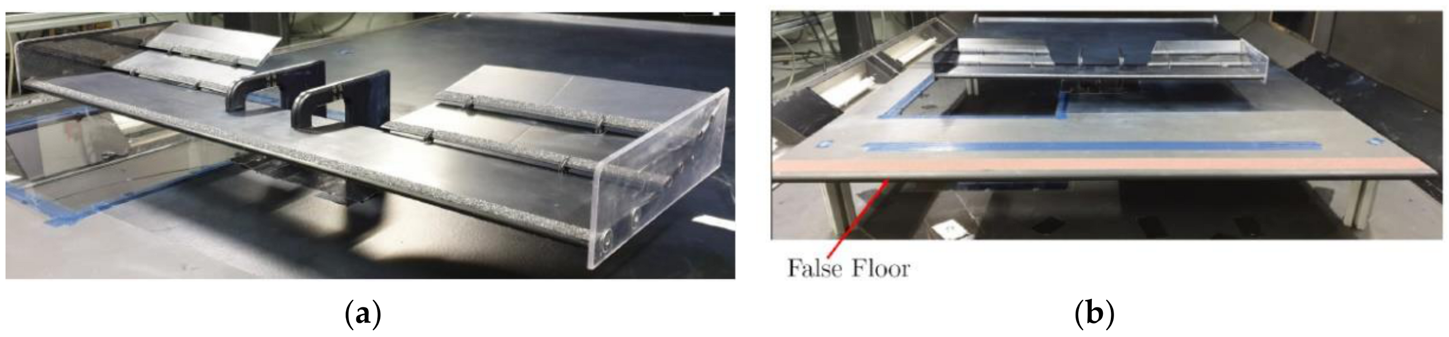
To ensure a flow structure representative of that produced by the many front wing designs used in the motorsport industry, a 50% scale generic wing was used as presented by Figure 1.
The wing consisted of a three-element, part-span flap design with flat endplates. The main-element is a NACA2412 profile with a chord length of 130 mm and an angle of incidence of 0°. Each flap is a Göttingen 795 profile with a chord length of 75 mm and an angle of incidence of 13° and 22° degrees respectively concerning the upstream and downstream flaps. The total chord length, c, is 270 mm with consideration of a 5 mm element overlap. The wingspan is 820 mm. Additional components such as the swan-neck mounts were required to connect the wing to the force-balance whilst small supports were attached between the wing elements to minimise aerodynamic deflection.
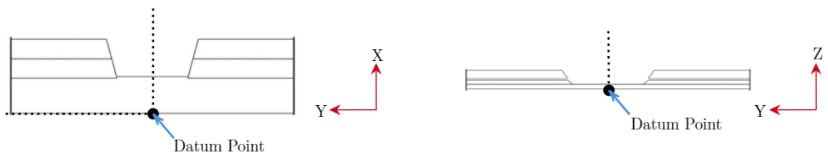
All cases were run at a ground clearance of 57.5 mm measured from the lower X-direction edge of the endplate to the ground; equivalent to 0.213 h/c. This ground clearance was selected based on a ground clearance sensitivity study to obtain the lowest ground clearance whilst ensuring the trailing vortex system remained intact. The datum point is presented by Figure 2.
As the numerical simulations assumed a fully turbulent boundary layer, grit strips featuring 35-micron particles were applied to the leading-edge of each element as shown by Figure 1a. Flow visualisation via flow-vis paint confirmed a fully turbulent boundary layer with the elimination of any laminar separation bubble.
2.1.2. Wind Tunnel
All experimental work was conducted using Loughborough University’s Large open circuit Wind Tunnel at a chord length-based Reynolds number of 0.55 × 10⁶. The dimensions of the working section are 1920 mm in width, 1320 mm in height and 3600 mm in length; more information on the wind tunnel’s specification can be found in [17]. This resulted in a blockage ratio of 4.3%.
As the working section does not feature a moving ground plane and a wing in ground effect demonstrates considerable sensitivity to the thickness of the ground boundary layer, a false floor was mounted above the tunnel’s ground plane as shown by Figure 1b. This is effectively a secondary floor that was mounted in the freestream flow i.e., above the boundary layer of the ground to ensure a thinner onset boundary layer is experienced by the wing.
To evaluate its effectiveness, a boundary layer velocity profile was gathered; importantly, this experiment was performed without the wing geometry to allow access for the transverse to which a Cobra probe was attached. The test was conducted at a freestream velocity of 30 m/s and the boundary layer was sampled at the location of the leading-edge of the wing. A comparison between the measured boundary layer and numerical boundary layer showed that the difference in boundary layer thickness between the two methods was determined as 4%. Further analysis using the numerical representation showed the displacement thickness to reduce from 6.5 mm to 1.9 mm at the onset of the wing geometry with the inclusion of the false floor.
The aerodynamic forces were measured using a six-component force-balance, sampled for 45 s excluding a flow settling time of 15 s; a larger sampling time was not required due to the inherent aerodynamic steadiness of the wing.
The freestream velocity used to normalise the aerodynamic forces was corrected using the MIRA blockage correction [18] as per Equation (1).
where BR is the blockage ratio in %.
This corrected freestream velocity was subsequently used to obtain the force areas of the wing as the following equations:
2.1.3. Stereo Particle Image Velocimetry (PIV)
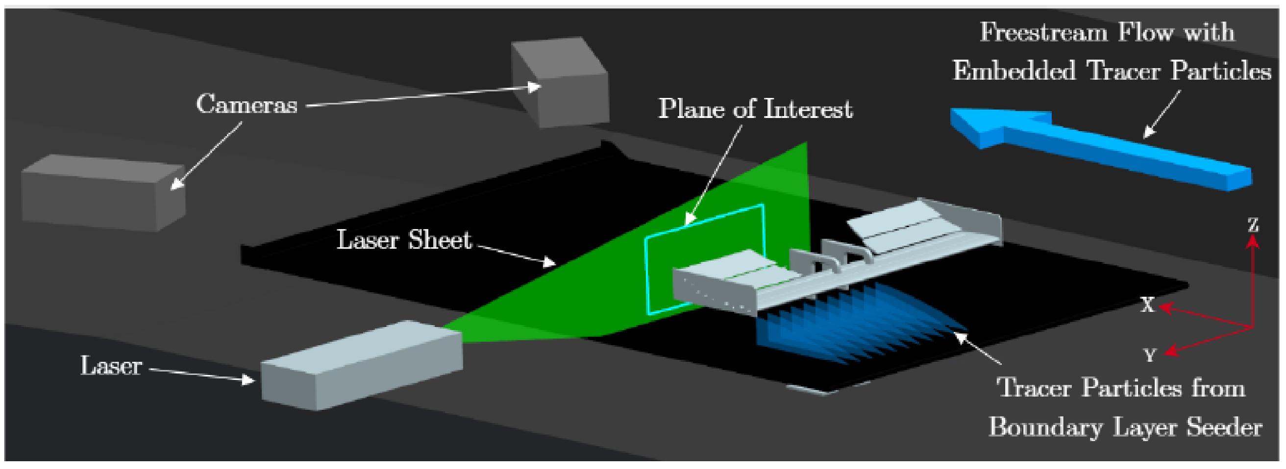
Stereo Particle Image Velocimetry (PIV) was selected to gather all cross-plane data in a setup illustrated in Figure 3. Tracer particles in the form of Di-Ethyl-Hexyl-Sebacat (DEHS) with a mean diameter of 1 µm were seeded into the freestream flow via a rake at the inlet of the wind tunnel as well as a boundary layer seeder located within the false floor. These particles were illuminated by a Litron 200 mJ Neodymium-Doped Yttrium Aluminium Garnet (Nd:YAG) double-pulsed laser. The images produced were captured via a pair of LaVision Imager ProX or LaVision SCMOS cameras (dependent on the resolution targeted) that were equipped with a tilt mechanism to take advantage of the Scheimflug principle upon which a Nikon Nikkor lens with a focal length of 50 mm or 105 mm (dependent on the resolution targeted) was attached with the aperture set to f# 4.
During the data acquisition of each PIV plane, 1000 image pairs were taken a sampling frequency of 2.5 Hz. This resulted in a total sampling time of 400 s. Once the raw images had been obtained, they were post-processed via a multi-pass scheme with an initial window size of 128 × 128 pixels with a square weighting and an overlap of 50%. This reduced to final window size of 24 × 24 pixels with a circular weighting and an overlap of 75%.
2.2. Numerical Methodology
2.2.1. Wing Geometries
To perform a numerical validation exercise, the model used in the experiment was recreated accurately in simulation. After the validation exercise, this geometry was scaled up to 100% for the main study. For the full-scale geometry simulations, the swan neck mounts and flap supports required in the experiment were removed to avoid complicating the simulations.
2.2.2. Computational Domain
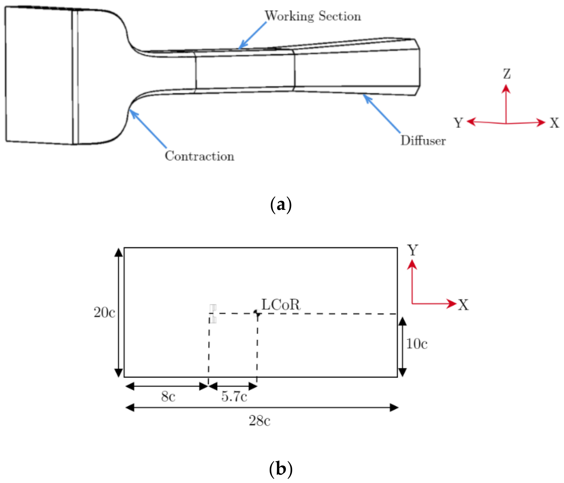
For the numerical validation, a partial model of the wind tunnel was used as shown by Figure 4a. For the main study the computational domain consisted of a rectangular geometry as presented in Figure 4b, giving a blockage ratio of 0.25%. For the straight-line condition, half-geometry simulations were performed to take advantage of the symmetry along the Y-axis; the blockage ratio, however, remained unchanged.
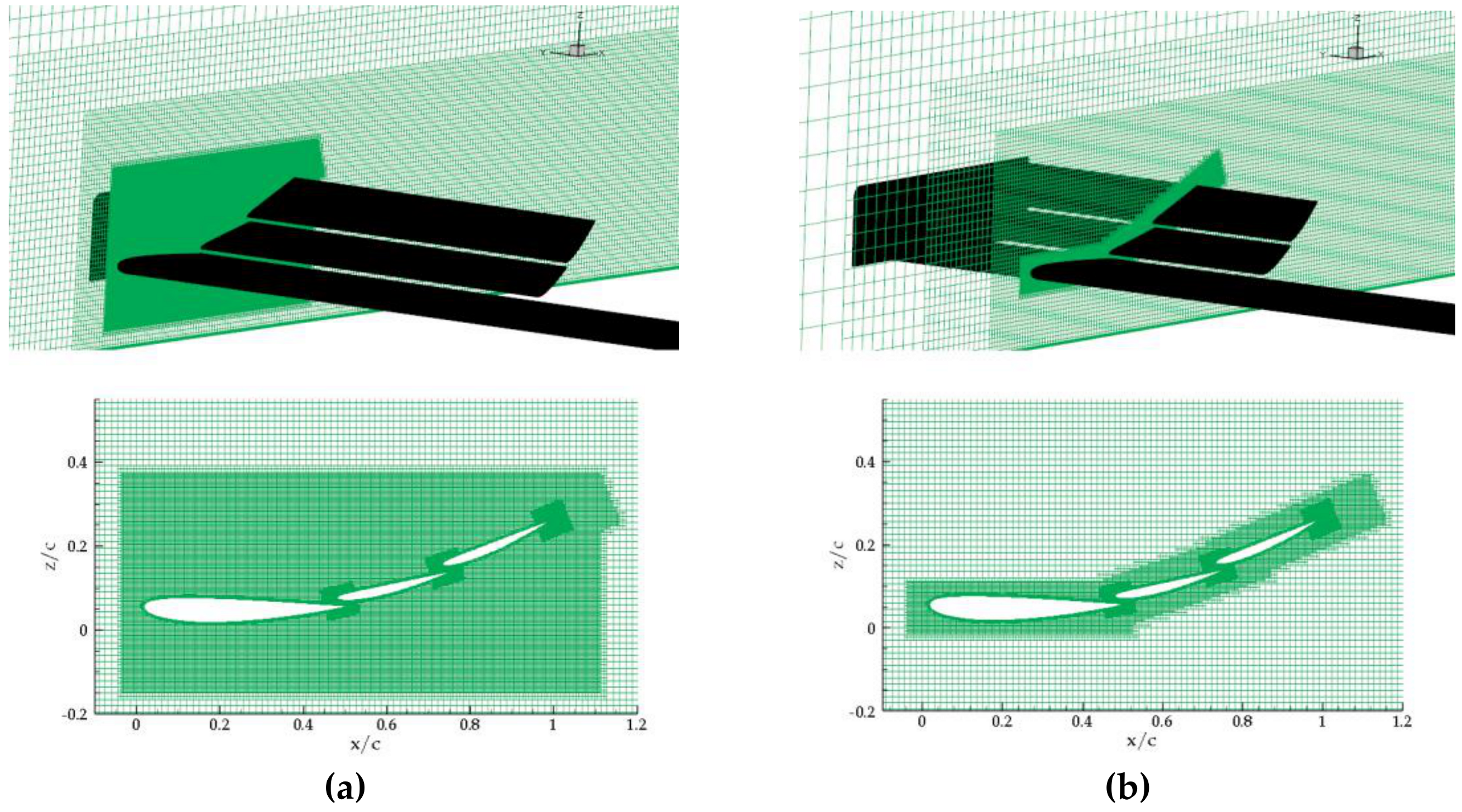
2.2.3. Meshing
The computational domain and its contents were discretised via structured hexahedral cells in conjunction with prismatic layers (Figure 5); the latter used to resolve boundary layers down to and including the viscous sublayer. The non-dimensional wall distance, y+, was <1 for all relevant surfaces. Before deciding the final mesh topology, a sensitivity study was performed to obtain mesh parameters that generate a flow solution that is no longer sensitive to increased mesh refinement. Regions of high vorticity were highly sensitive to mesh resolution and thus required an increased cell count. The final mesh for the numerical validation case consisted of 34 million cells. Concerning the full-scale geometry simulation, the cell size was scaled by 2× to ensure consistency with the half-scale counterpart and resulted in a cell count of approximately 58 million cells for the full-geometry simulation and hence equated to 29 million cells for the half-geometry simulation.
2.2.4. Physics Modelling
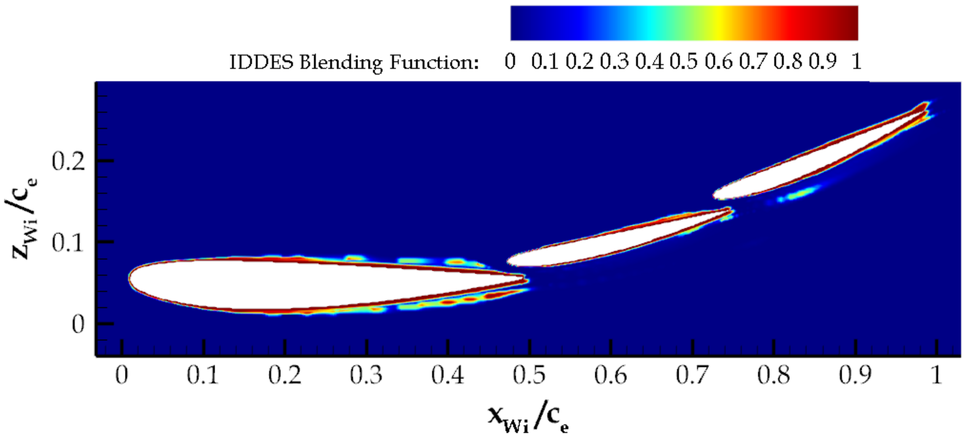
All simulations adopted the Detached Eddy Simulation (DES) approach under the implicit time model with the k-ω SST turbulence model. DES is a hybrid approach between Reynolds-Averaged Navier-Stokes (RANS) and Large Eddy Simulation (LES); the former was used to resolve attached flows whilst the latter resolved unsteady flows [19]; an example of such is shown by Figure 6 where the boundary layer is resolved via RANS whilst LES is adopted away from the surface thereby yielding the benefit of avoiding excessive dissipation of vortices which is commonly associated with RANS. The second-order upwind/central differencing convection hybrid scheme was applied for the numerical discretisation and the Semi-Implicit Method for Pressure Linked Equations (SIMPLE) was utilised as the pressure-velocity coupling algorithm; more information on such can be found in the STAR-CCM+ documentation [19].
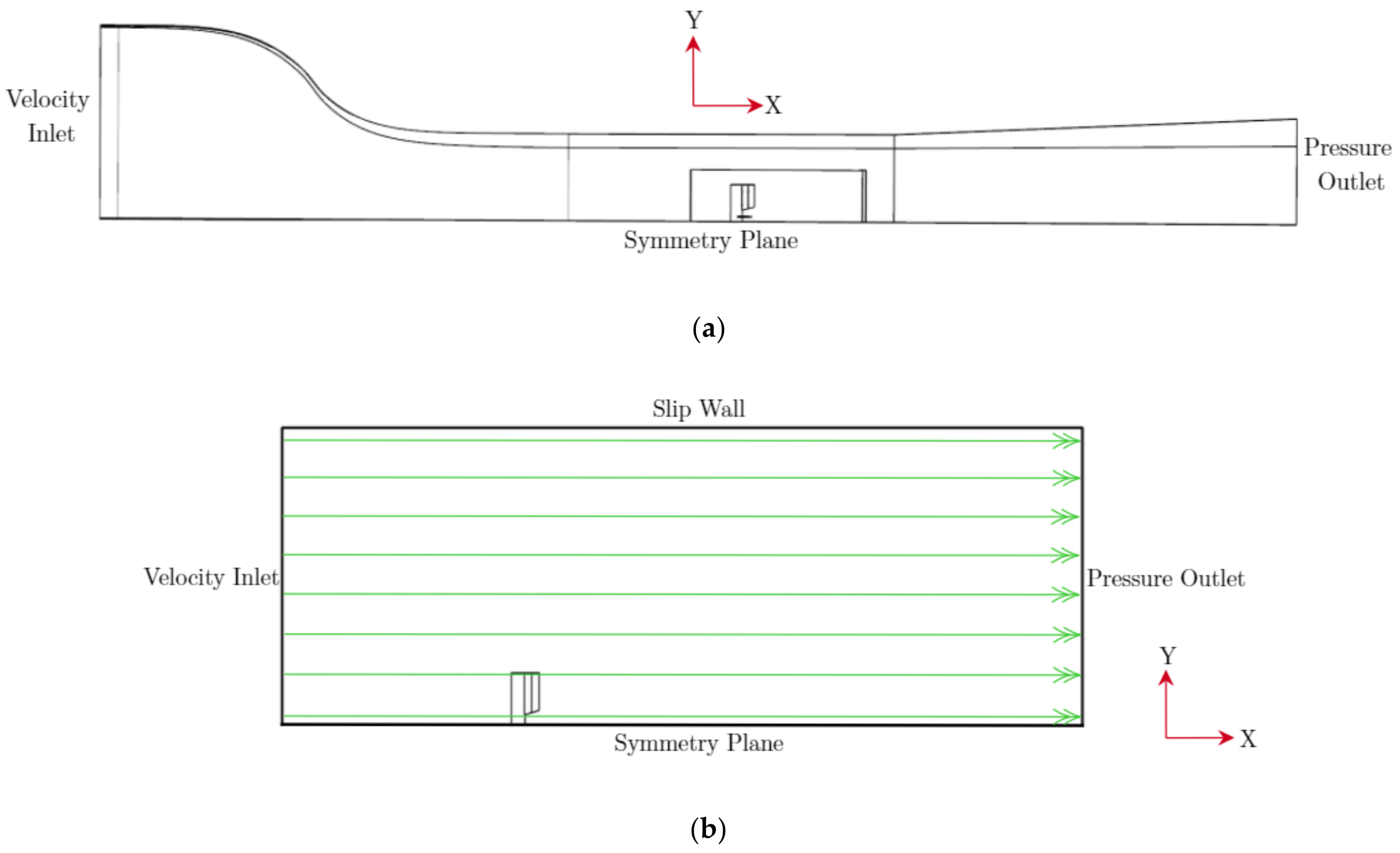
Regarding the numerical validation case, the boundary conditions presented by Figure 7a were applied. The velocity inlet was set to 4.05 m/s, as the contraction ratio is 7.4 this resulted in the desired working section freestream velocity of 30 m/s. All walls were assigned a no-slip condition to match the experimental conditions.
For the main study, conventional boundary conditions were applied as shown by Figure 7b. The ground plane was set as a moving, no-slip wall with its velocity corresponding to the freestream velocity whilst the “roof” was set to a slip wall to eliminate the effects of viscosity; the wing surfaces were assigned as no-slip walls. Whilst the flow is never perfectly symmetric, the symmetrical wing geometry was operating in a symmetrical flow-field in the straight-line condition and importantly, was not a bluff body. Therefore, minimal macro-scale asymmetry was present even in the case of the instantaneous wake and hence a symmetry plane was assigned to take advantage of this and thus reduce unnecessary computational expense. At the inlet, the velocity magnitude was set to zero in the absolute reference frame. Instead, to induce a non-zero freestream velocity through the domain, the Rigid Body Motion (RBM) technique in the form of translational motion of 22 m/s in the -X-direction was applied. This led to a chord-length based Reynolds number of 0.8 × 10⁶. This method is discussed in further detail shortly.
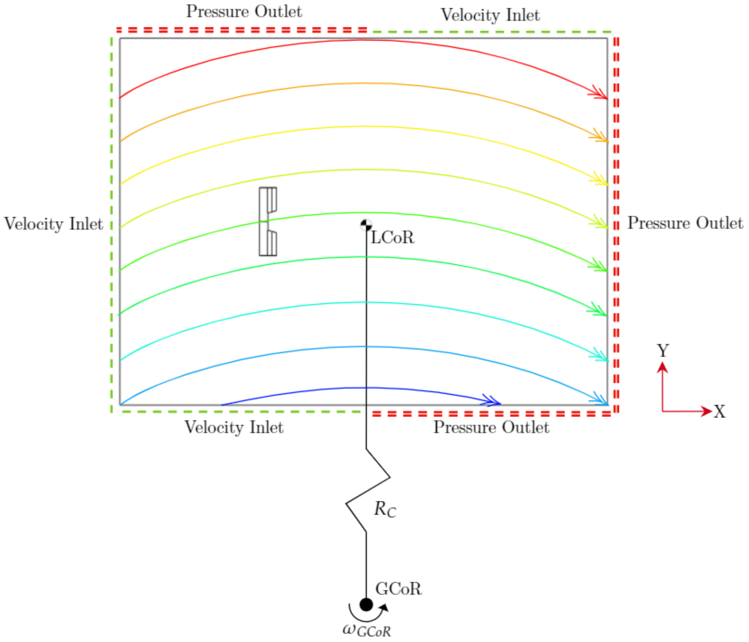
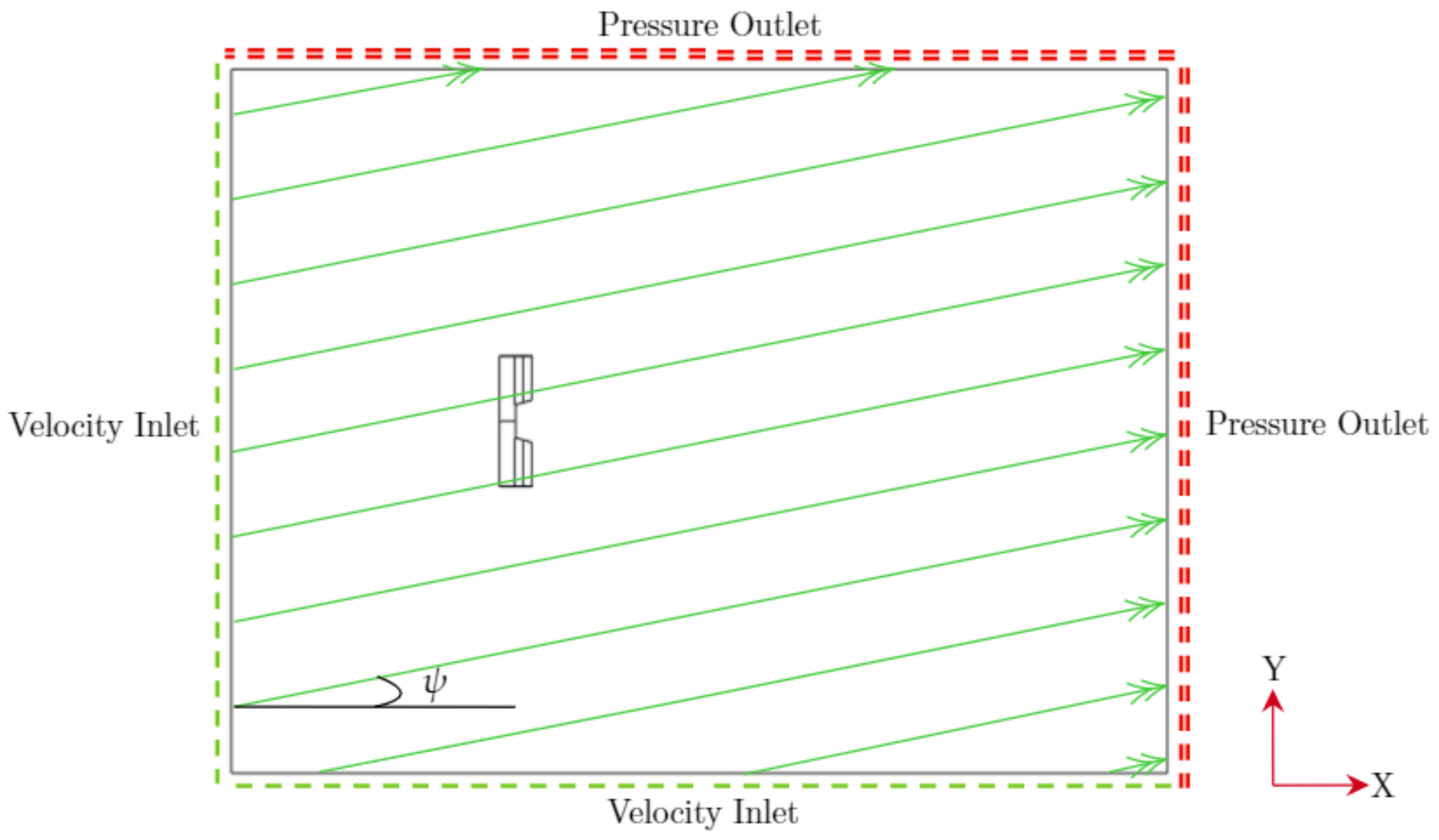
The cornering condition requires the consideration of both the topology of the computational domain and the simulation of motion. Regarding the topology, either a rectangular computational domain or a curved domain must be selected with the associated boundary conditions, as discussed in [20]. Whilst it is easier to apply the appropriate boundary conditions with a curved domain, it does not allow the simulation of multiple corner radii via the same domain or mesh nor does it allow the simulation of multiple operating conditions such as the straight-line condition. Therefore, a rectangular domain was used and the boundary conditions assigned for this are shown in Figure 8. Similarly to the straight-line condition, the velocity at the inlets was set to zero in the absolute reference frame. The ground plane was set as a moving, no-slip wall with it rotating in the opposite sense to the motion of the domain in the relative reference frame. The pressure outlets were specified a uniform gauge pressure 0 Pa relative to the atmospheric pressure of 101,325 Pa.
For the simulation of motion, the domain is required to rotate about an external point represented as the Global Centre of Rotation (GCoR). Typically, three methods are available to simulate this rotation: a moving reference frame (MRF), the Rigid Body Motion (RBM) or the overset mesh. The overset approach allows for complex combinations of motion but introduces extra computational cost and complexity. The MRF approach simulates motion by adding a grid flux term to the conservation equations whilst keeping the mesh stationary. However, MRF is not recommended for unsteady flow solutions [21]. Therefore, the RBM technique was used in which the grid flux was calculated based on the prescribed displacement of the entire mesh at each time-step. This method is an alternative to the overset mesh technique that avoids the interpolation errors associated with the latter. The front wing was positioned 5.7c forward of the assumed location of the centre of mass of the race car, denoted as the Local Centre of Rotation (LCoR) in Figure 8. The angular velocity at the GCoR (ωGCoR) was set such that the tangential velocity at the LCoR i.e., the reference velocity, matched the freestream velocity set for the straight-line condition; based on a corner radius of 20 m. Larger corner radii were also simulated but a corner radius of 20 m demonstrated the effects of cornering in the most pronounced fashion.
The fixed yaw condition is also reliant on the motion of the domain, in this case the RBM method with translational motion in both the -X direction and -Y direction was applied with the velocity magnitude equating to the freestream velocity in the straight-line condition. The boundary conditions are shown by Figure 9. The yaw angle was set to 8.75°, based on the local yaw angle at the datum point of the wing during the 20 m radius cornering case.
2.2.5. Temporal Discretisation
The time-step used for the simulations was set at 2.3 × 10⁻⁵ s for the validation case and 6.273 × 10⁻⁵ s for the main study, to ensure that the Courant-Friedrichs-Lewy (CFL) number was <1 in all regions of interest. The number of inner iterations was set to 5 after sampling the velocity and pressure at various locations within the flow-field to determine the minimum number of iterations required for convergence at a particular time instant. The flow solution was time-averaged for 30,000 time-steps, initiated after a physical time of 0.5 s to allow the flow to develop.
2.2.6. Post-Processing
In line with the relative simplicity of the straight-line and fixed yaw conditions, the direction each force vector was defined as per Figure 10. It must be noted that the force coefficients in the wind axis (WA) are also presented for the fixed yaw condition as further information.
These forces were subsequently normalised by dividing them by the dynamic pressure allowing for force area to be obtained as per the following equations:
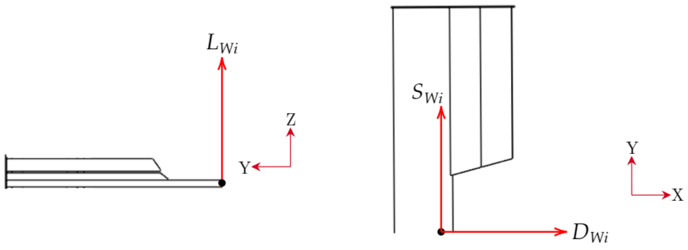
The drag force vector was defined as the force opposing the heading motion/velocity of a body. Thus, it was aligned to the tangent of the body’s path whilst the side-force, by definition, as the force acting orthogonally to the drag force; as illustrated in Figure 11. This follows Keogh et al. [20] and Keogh [22], that the drag force is linearly proportional to the moment acting about the GCoR (MDWi) to oppose the circular path of the body. The lift force vector is unaltered.
To implement this method within CFD, the drag force is computed using Equation (7) as adopted by Joseffson et al. [23].
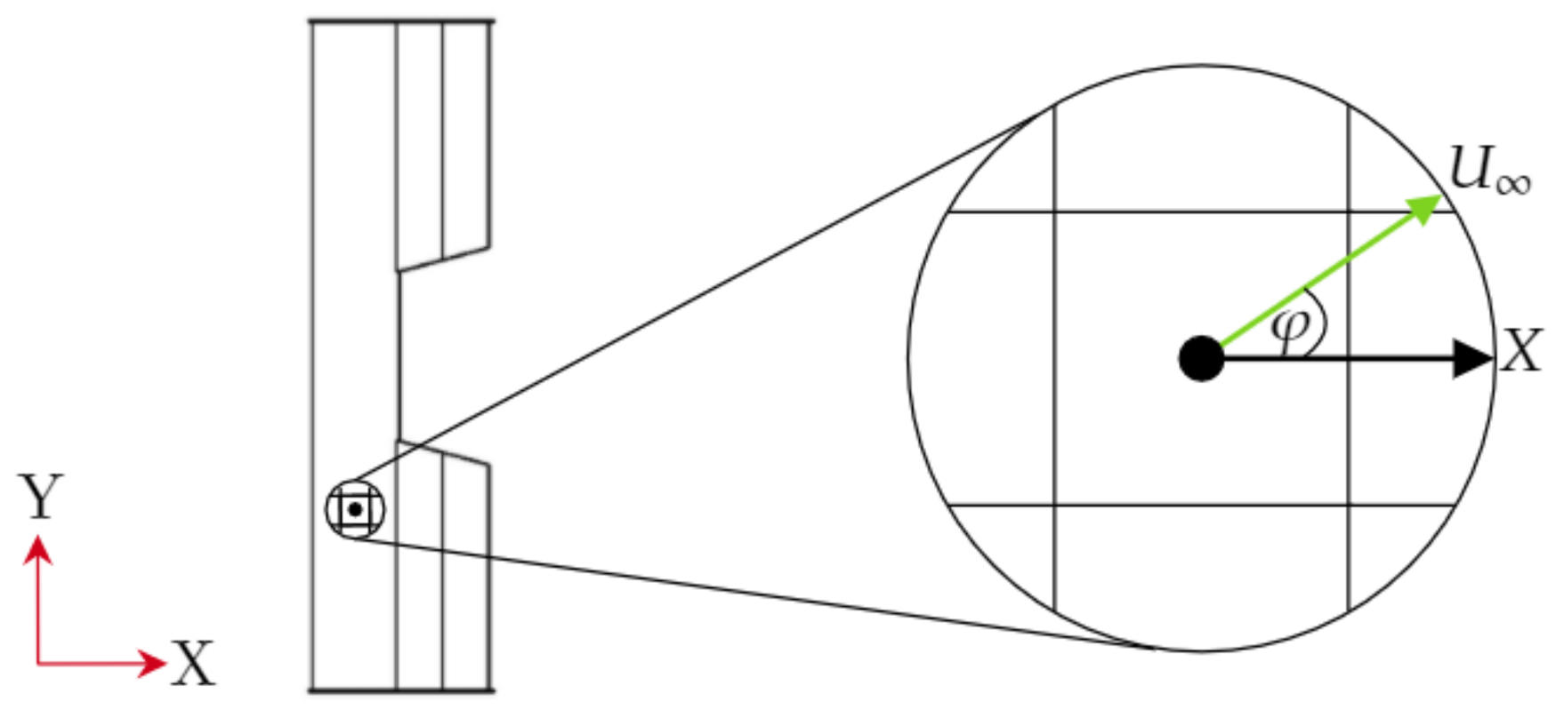
where P is the pressure, A is the cell area., is the wall shear stress and is the local yaw angle between the flow and the X-axis at a cell’s location as per Figure 12.
Once the contribution of each cell was determined, the total drag force was obtained via the summation of these incremental contributions as per the Equation (8).
where N is the number of mesh cells associated to the wing’s surface.
Similarly, the method was applied to obtain the side-force as per Equations (9) and (10).
Due to the spatial variation of the freestream velocity, normalization via a constant freestream velocity is likely to lead to confusion in the results. Instead, the freestream velocity, based on distance from centre of rotation, at the location of each mesh cell, , was utilised. Therefore, similarly to Josefsson et al.’s [23] method to calculate the drag force, the force coefficients were calculated on a cell-by-cell basis before each incremental contribution was summed to obtain the total force area coefficient of lift, drag and side force as per the following equations.
Whilst in the existing literature the total pressure data is presented in the form of a coefficient, a more intuitive method is to a present a percentage of total pressure loss by comparing the effects on total pressure of the presence of the geometry in the computational domain relative to an empty domain on a cell-by-cell basis. This gives insight into the effective energy change within the flow-field and, allows a direct comparison across the operating conditions despite the freestream total pressure variation present in the cornering scenario. Equation (14) was used to compute this.
where is the total pressure with geometry placed in the domain and is total pressure in an empty domain.
The vorticity of the flow-field was calculated via the inclusion of all vorticity components resulting in the magnitude of vorticity to be presented. This was subsequently normalised by taking into account the chord length of the wing, c or ce (the latter used for the numerical validation case) and the freestream velocity as per Equation (15); for the cornering condition, the reference freestream velocity was used.
3. Results & Discussion: Numerical Validation
A comparison of the forces generated in the experiment and simulation, are presented in Table 1. The numerical solution overpredicts downforce by 3% whilst drag is underpredicted by 3.7%. Besides numerical errors, there was slight deflection of the flap elements in the experiment, with this most pronounced in vicinity of the inboard tips resulting in a reduction of effective camber that may be responsible for some difference in lift. Furthermore, the grit strips applied to the leading-edges may have resulted in a reduction in peak suction as well as increased drag. Overall, this results in the wing efficiency to be overpredicted by 7%. However, the agreement between the experiment and simulation is very good.
The formation of endplate vortices (Figure 13) shows broadly good correlation between the experimental and simulated flow field. The top endplate vortex is underpredicted by 9% and laterally located 0.7% further away from the wing’s centreline and elevated by 4%. The peak vorticity magnitude of the bottom endplate vortex is also underpredicted by 7% and it is located 0.6% further away from the centreline and elevated by 33% relative to that observed under the experimental conditions equivalent to 0.009 h/ce.
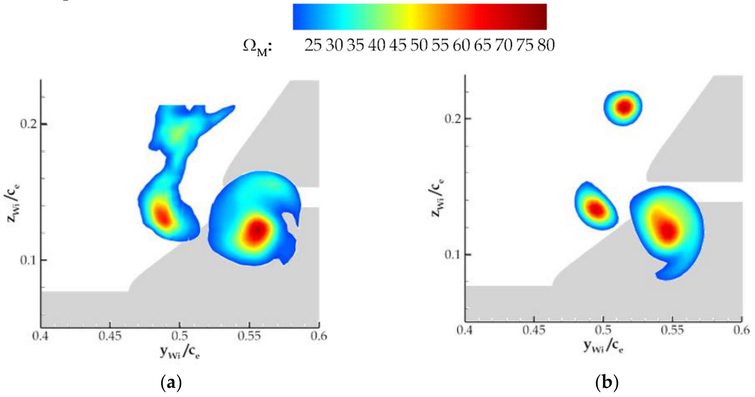
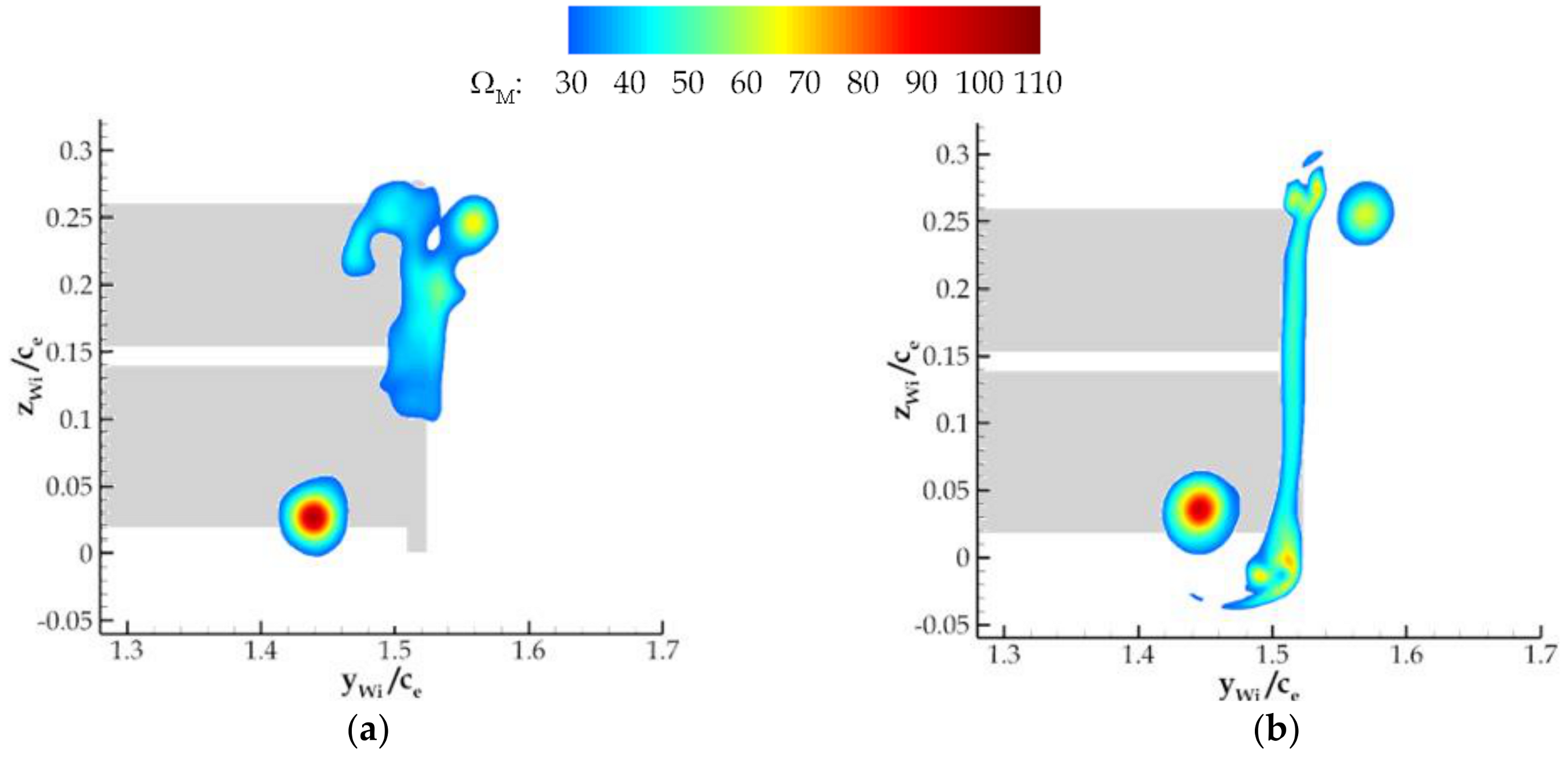
The inboard flap tip vortex also shows good agreement with the three vortex cores measured being present in the numerical solution (Figure 14). However, minor discrepancies are observed. For example, the numerical solution underpredicts the largest vorticity patch from a size and strength context. The patch on the left of this is in better agreement but its size again is underpredicted whilst its strength is overpredicted. The largest discrepancy, however, is demonstrated by the uppermost patch which is much more regular in shape and consists of more vorticity than that demonstrated by the experiment. Also, the beginnings of vortex merger of such with the lower patch is not observed. It is also laterally positioned further away from the wing’s centreline and further away from the ground. Note that the downwards deflection of the flaps in the experiment may be responsible for much of this discrepancy alongside the grit strips applied to the leading-edges of the flap elements.
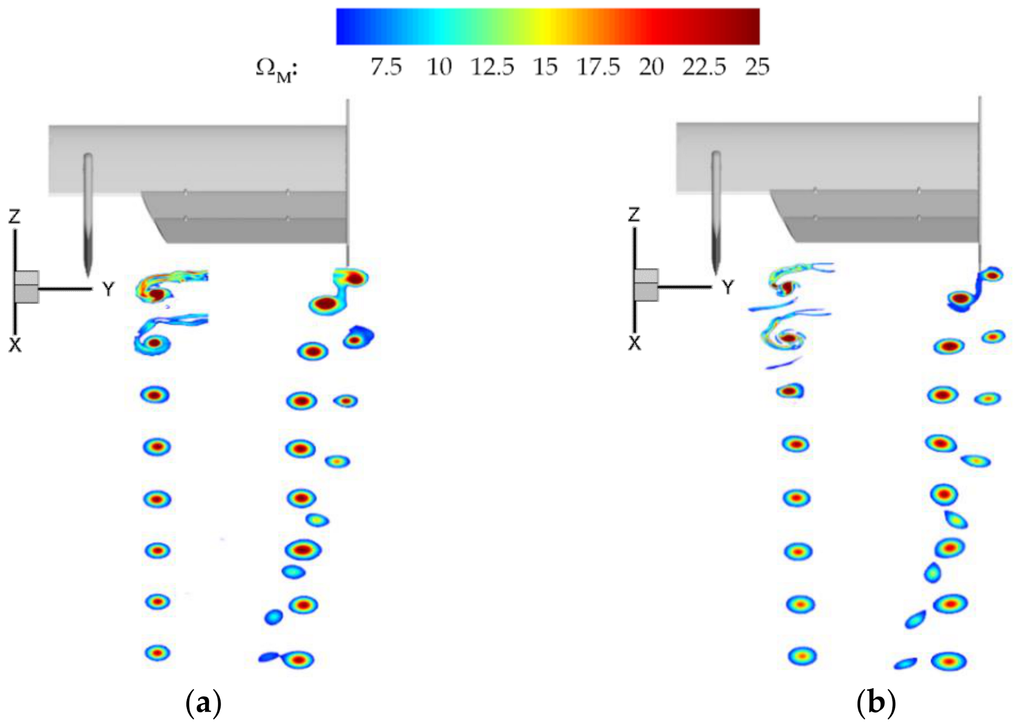
Concerning the downstream behaviour of the trailing vortex system, as presented by Figure 15, good agreement was observed for their position as well as the merger of the endplate vortices. However, all vortices were relatively displaced further away from the centreline of the wing with downstream distance in the numerical solution. The dissipation rates of the inboard flap tip vortex and the bottom endplate vortex were also significantly larger in the numerical solution.
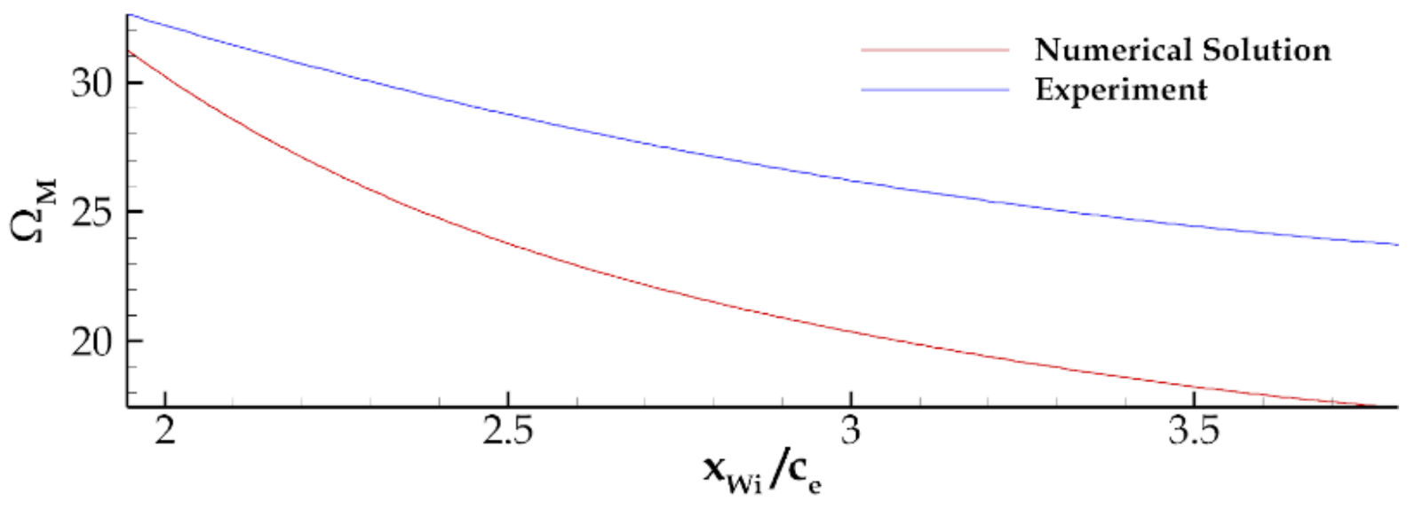
Focusing on the inboard flap tip vortex as this was a single, isolated vortex with minimal influence of the other vortices, Figure 16 demonstrates the ever-increasing discrepancy in vorticity magnitude with downstream distance; at xWi/ce = 1.944 was 5% but grew to 36% at xWi/ce = 3.796. The dissipation of vortices tends to be rapid in general purpose CFD codes [19] and thus for this study was unavoidable without an unfeasible increase mesh cell count.
4. Results & Discussion: Comparison of Straight-line, Cornering & Fixed Yaw Conditions
With the accuracy of the numerical methodology demonstrated in the previous section for the 50% scale model, it is now applied to the full-scale case to investigate the differences seen in straight-line fixed yaw and cornering conditions.
4.1. Cornering Flow-Field Characteristics
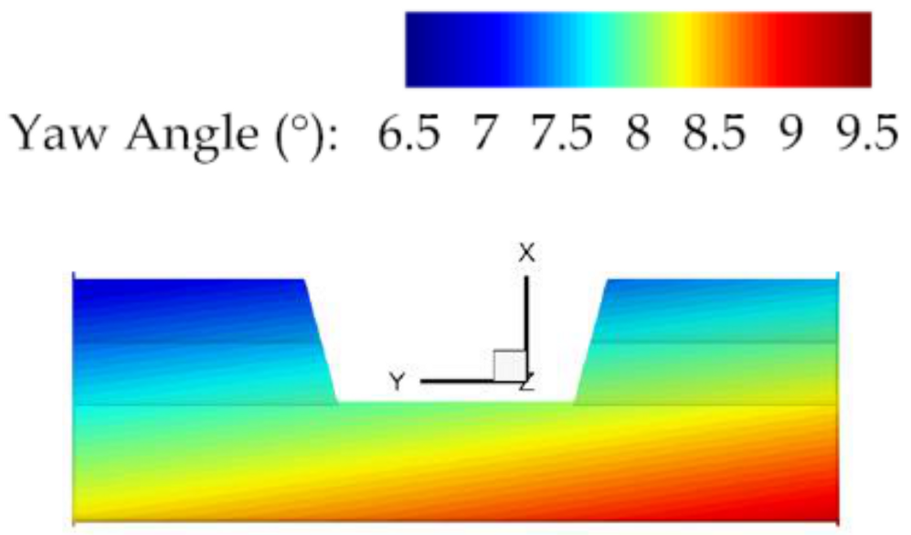
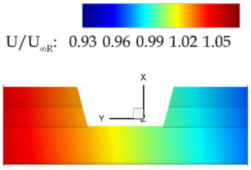
The cornering condition consists of a combination of two aspects: the varying approach angle of the oncoming freestream flow resulting in a curved flow as well as variation in freestream velocity. From a yaw angle perspective, (Figure 17), the most extreme yaw angle is located at the leading-edge of the inboard endplate; this gradually reduced away from this region. A maximum yaw angle variation of 2° is observed across the surface of the wing.
The freestream velocity, (Figure 18), results in the outboard region of the wing experiencing a greater freestream velocity relative to the inboard region with a variation of up to 5% across the wingspan. A further consequence of this was the outboard region experiences a greater total pressure and hence energy relative to the inboard region. This was because the freestream static pressure remains constant whilst the dynamic pressure was found to increase.
4.2. On-Surface Pressure Distribution
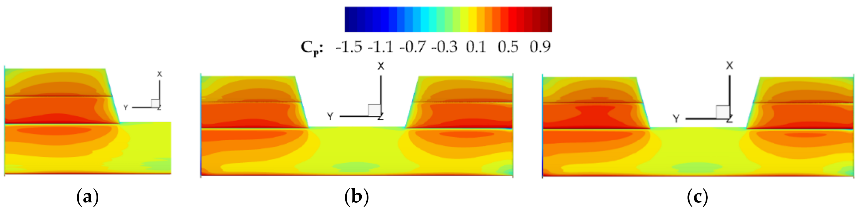
The surface pressures under the straight-line condition, illustrated by Figure 19a, shows the higher pressure is most intensely concentrated in the mid-span region between the inboard tips of the flaps and the endplate; this being the region where three-dimensional effects are the least intrusive. Away from this region, the pressure progressively reduces as the flow accelerates towards regions of lower pressure via an increasing spanwise velocity component.
The introduction of the cornering (Figure 19b) and fixed yaw conditions (Figure 19c) results in an asymmetrical pressure distribution with the former demonstrating this to a greater degree. The first and largest contributor unique to the cornering condition is the varying freestream total pressure. This results in the overall pressure magnitudes to be greater on the outboard surfaces relative that in a straight-line condition whilst the opposite occurs on the inboard side. Specifically, this behaviour is due to the variation in the amount of potential energy available because of the total pressure variation.
The second contributor is associated with the behaviour in the vicinity of the endplates, where the impact of yaw is dominant and is therefore also present in the fixed yaw condition. The inner face of the outboard endplate sees a notable increase in pressure due to this face representing the windward side. This subsequently impinges on both the main-element and upstream flap with it most pronounced on the former. A region of significant pressure loss is also located within the first quarter of the main-element’s chord length at the inboard junction between the main-element and endplate. This is attributed to the flow acceleration around the leading-edge of the endplate from its outer face to its inner face resulting in a suction peak that impinges on the main-element.
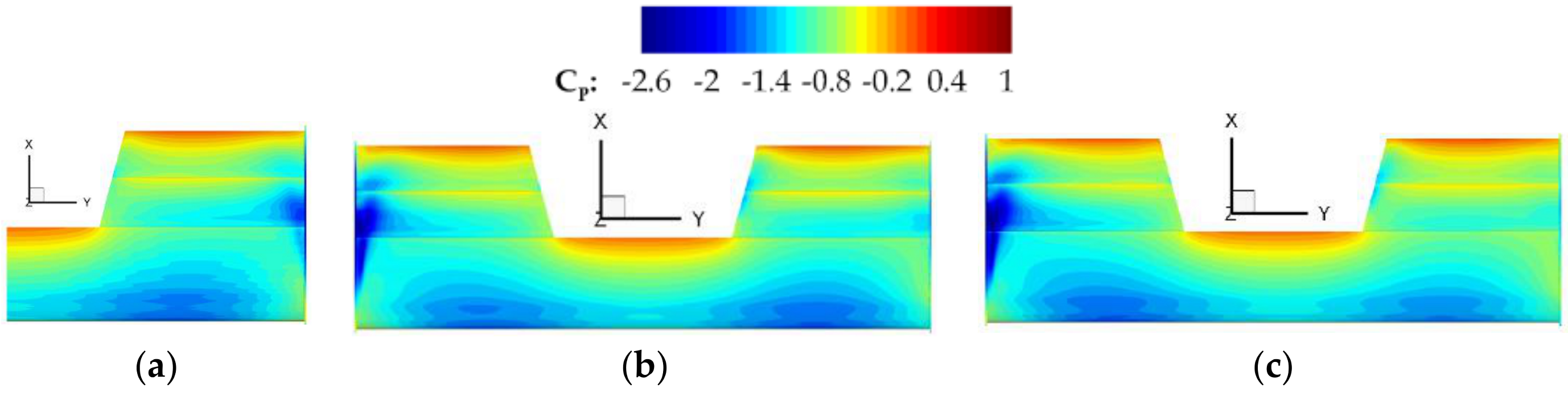
Moving onto the suction surfaces under the straight-line condition, (Figure 20a), in the central main-element section where there are no flaps, suction is notably weaker compared to the region under the influence of the flaps. This demonstrates the circulation benefit of a multi-element design over a single-element design as per Smith [24]. Where there are flaps, the most intense suction is situated between the inboard tips of the flaps and the endplate. This suction is also strongly biased towards its leading-edge due to the aerofoil profile and the absence of a slat element. Downstream of this region, pressure recovery is demonstrated in agreement with Van den Berg [25]. Towards the endplate, a region of intense suction is noted which is attributed to the impingement of the low-pressure core of the edge vortex [15].
Similarly to the pressure surfaces, for the cornering condition, one of the main contributors is the varying freestream total pressure. This results in greater suction to be achieved on the outboard region of the wing relative to that observed in a straight-line condition whilst the opposite occurs on the inboard region. However, it is no longer the largest contributor towards the asymmetry.
Instead, the effect of yaw is recognised as being the dominant contributor and is shared with the fixed yaw condition. On the outboard side of the cornering wing, the region of intense vortex-induced suction is substantially reduced in comparison to when in a straight-line condition. This is because the reduced pressure imbalance between the inner and outer faces of the endplate leads to the weakening of the bottom endplate vortex. Conversely, the inboard side experiences a substantially increased vortex-induced suction.
Furthermore, in the region where the inboard tip vortex is generated, an additional patch of suction is observed on the outboard of the wing. This is of greater intensity than when in a straight-line condition whilst the converse is true in the region where inboard tip vortex is generated. The additional patch of suction is vortex-induced because the trajectory of the freestream flow, draws the vortex directly under the flaps. This leads to a notable region of pressure impingement.
The main discrepancy between the fixed yaw and the cornering conditions, is that away from the endplates, suction is found to be greater on the inboard side of the wing relative to the outboard side under the fixed yaw condition. This is attributed the respective strengthening and weakening of the inboard and outboard bottom endplate vortices, and the associated pressure impingement that results in an asymmetric pressure distribution between the two regions; this being also true under the cornering condition. However, the absence of the varying freestream total pressure under the fixed yaw condition results in the outboard side of the wing generating lesser suction whilst generating more suction on the inboard side of the wing.
4.3. Force Analysis
The forces generated by the wing under all the operating conditions are presented in Table 2.
A reduction of only 0.4% and 0.5% in downforce is noted for the cornering and fixed yaw conditions respectively relative to the straight-line condition. The drag increases by 5% in the cornering condition relative to the straight-line condition. Whilst the lift-induced drag plays a small role, the increase of drag is predominantly due to the influence of the endplates; where the pressure distribution in the vehicle axis would be incorrectly interpreted as side-force, but here contributes to drag. The wing efficiency meanwhile is reduced by 5%. The fixed yaw condition also sees a drag decrease of 1%. This is chiefly due to the increased strength of inboard bottom endplate vortex being more than outbalanced by the decrease in the suction of its outboard counterpart leading to an overall decrease of induced drag. In this case the wing efficiency increases by 0.5%.
Both the cornering and fixed yaw conditions introduce a non-zero side-force. However, the cornering condition produces a side-force 33% less than the yaw condition. This is largely due to the interpretation of the direction of the force vectors which are not common between the two conditions. Whilst only the endplates contribute towards the side-force in the fixed yaw condition, in the cornering condition both the pressure and suction surfaces of the wing elements generate a force that results in a negative wind-axis side-force whilst the pressure distribution on the endplates acts in the opposite direction creating a positive wind-axis side-force; ultimately, this results in the reduction of the absolute side-force magnitude. However, when presented in the wind-axis, the drag and side force for the fixed yaw case show good agreement with that for cornering. This suggests that if a suitable fixed yaw angle is chosen, e.g., based on the local yaw angle of the datum point of the wing during cornering, then representative data for forces experienced during the corner can be obtained from a fixed yaw test for an isolated wing.
4.4. Off-Surface Flow-Field
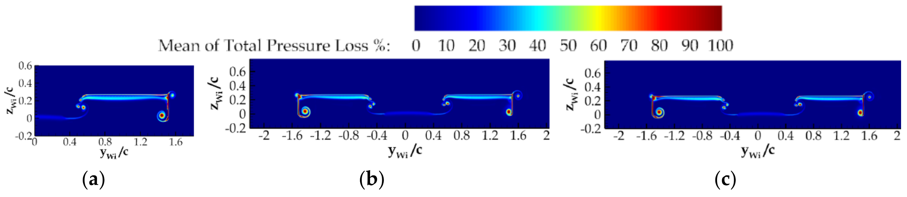
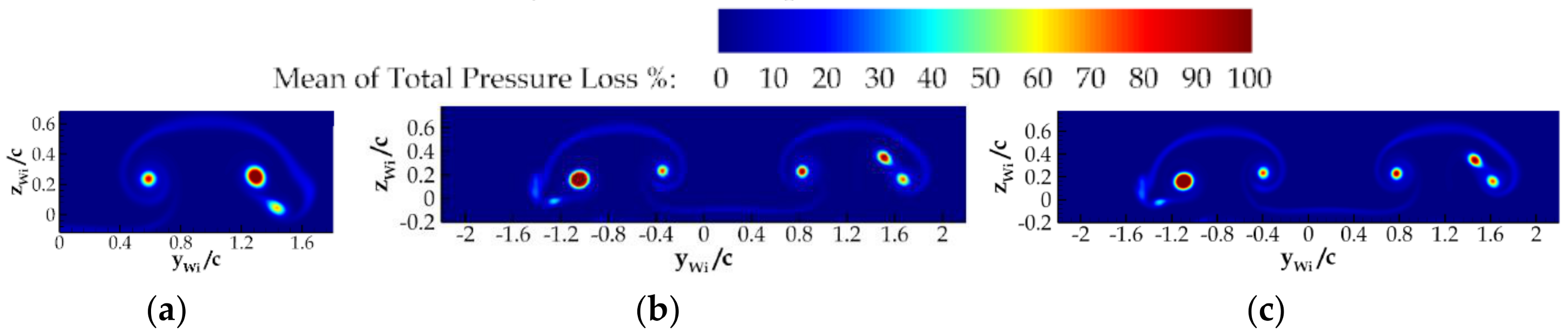
The off-surface flow-field is dominated by the shear layer shed directly from each wing element and the trailing vortex system as presented by Figure 21a. The shear layer production is dominated by the main-element both in thickness and the intensity of the energy loss; this is in agreement with Zhang et al. [9] and Soso et al. [13]. This behaviour is largely unaltered under the cornering and fixed yaw conditions.
Further downstream, (Figure 22a), the shear layer from each element is unifies into single region of energy deficit. This unified shear layer wake mixes and diffuses into the undisturbed freestream flow with its energy loss decreasing and its thickness increasing in agreement with Zhang et al. [12]. Furthermore, due to the induced velocities of the trailing vortex system, a proportion of this wake is pulled towards the vortices leading the overall shape of the wake to resemble an inverted “U”.
Under both the cornering and fixed yaw conditions, notable differences from the straight-line case are observed, one of which is that the wake is shifted outboards to coincide with the direction of the freestream flow and the path of the trailing vortex system. Other differences are ascribed to the variation in the vortex strengths within this system and their associated induced velocities as well as the accelerated merging of inboard endplate vortices. The single salient difference between the cornering and fixed yaw conditions is that the wake is shifted outboard more aggressively for the latter as per the trajectory of the freestream flow.
4.4.1. Formation of the Trailing Vortex System
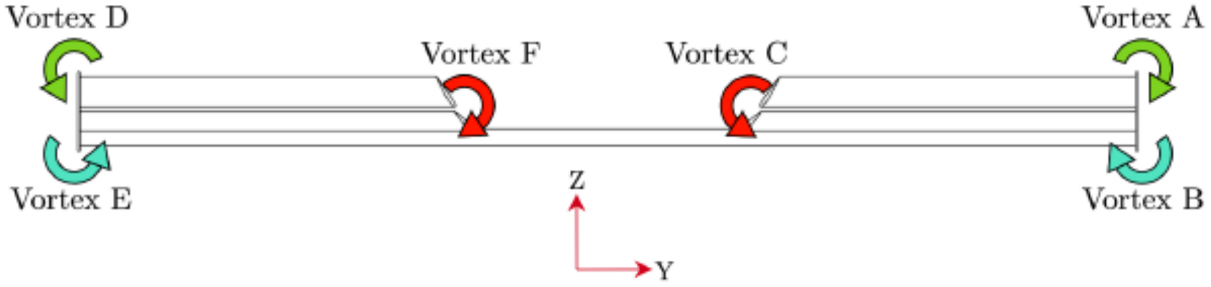
To aid in the explanations, the vortices within the trailing vortex system of the wing have been labelled as shown by Figure 23.
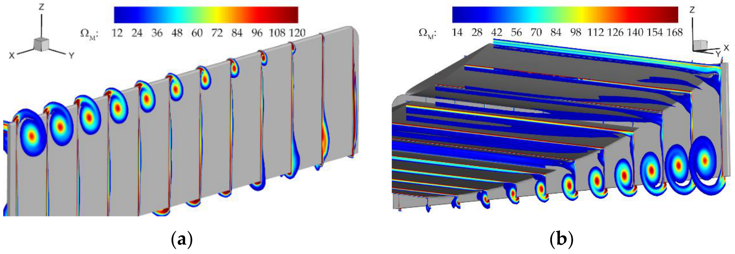
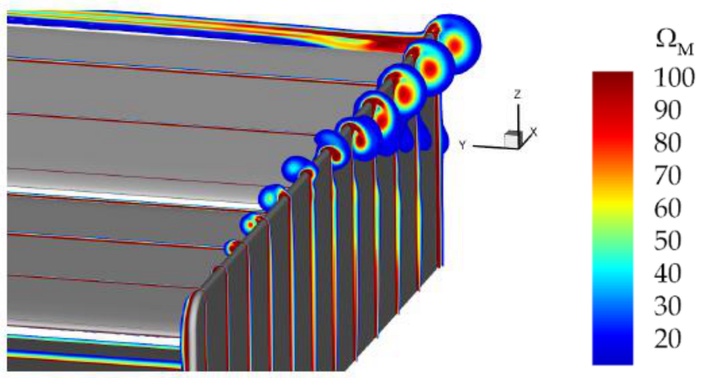
Both Vortex A and Vortex B form because of a spanwise velocity component. As per Figure 24, the separated shear layers caused by this curl up to form circular, coherent and regular vortices. With increasing chordwise distance from the leading-edge of the endplate, these vortices are continuously fed by the separated shear layer leading to an increase in diameter of the vortices.
Whilst the vortices are, overall, formed through an identical process to that under a straight-line condition, the formation of Vortex D is altered for both the cornering and fixed yaw conditions; an example using the cornering condition is demonstrated by Figure 25. An initial vortex is formed on the inner face of the inboard endplate due to the higher pressure of the outer compared to the inner face of the endplate due to the local yaw. As the pressure increases downstream via the flaps, the direction of the pressure gradient is reversed, and Vortex D begins to form. Consequently, the initial vortex dissipates with its residue being consumed by Vortex D.
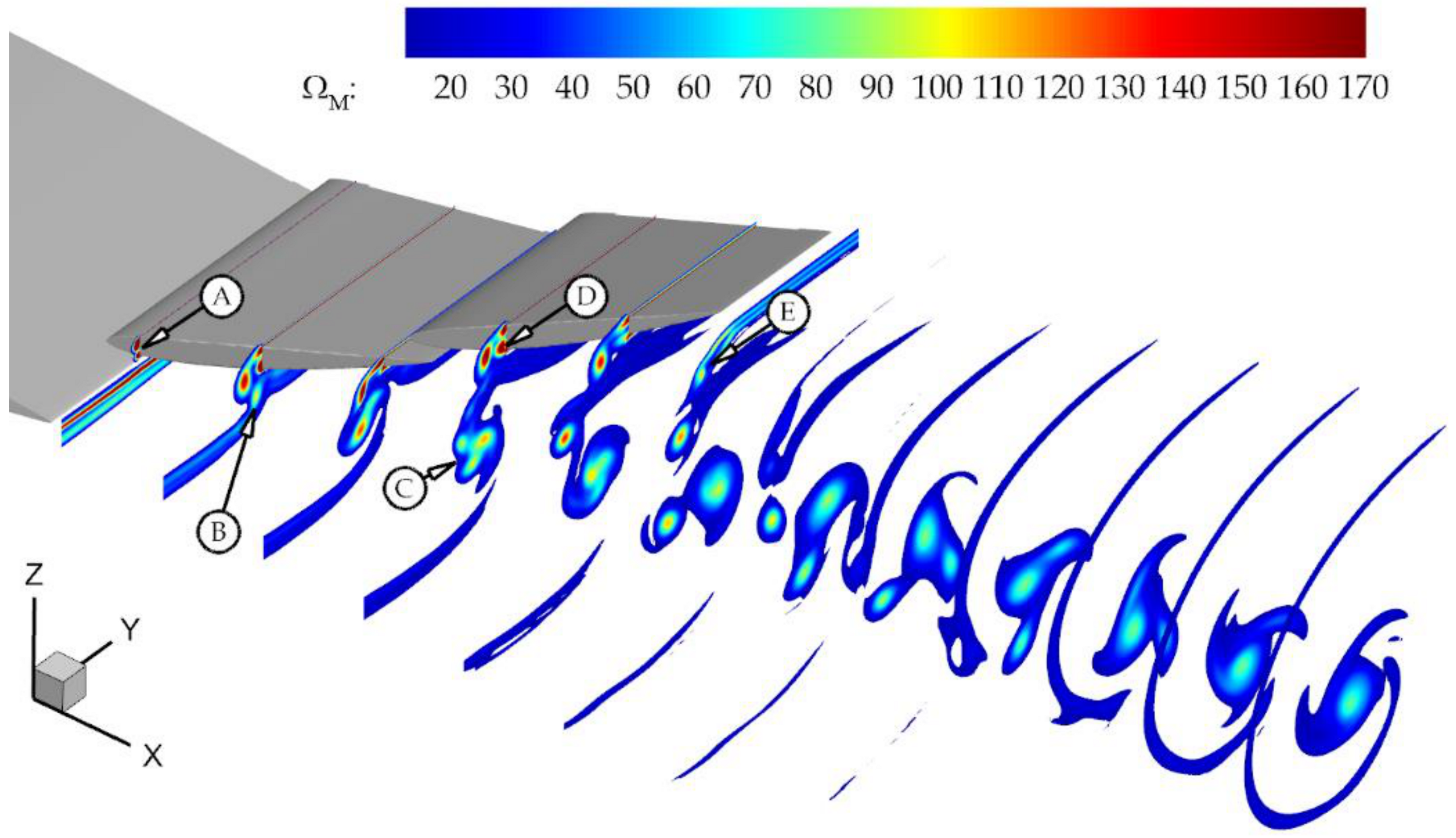
The formation of Vortex C is considerably more complex as it is the product of multiple patches of concentrated vorticity that the free shear layer wraps about, (Figure 26). Beginning at (A), an initial pair of counter-rotating patches of vorticity is formed; these are attached to the inner face of the upstream flap just downstream from its leading-edge. Downstream of this point, as the mainstream flow curled over, the patch of vorticity with the same sign is augmented whilst the other patch is dissipated. The induced motion of the augmented vorticity patch leads to the rotation of the separated shear layer from the trailing-edge of the main-element - to the extent that a second patch of co-rotating vorticity is formed denoted by (B). At the mid-chord point of the flap, the augmented patch of vorticity breaks away from the inner face of the flap and merges with the second patch of vorticity. From this point to the trailing-edge of the flap, two more patches of co-rotating vorticity form and detach from the inner face of the flap in a sequential manner. These begin to merge with the “main” patch of vorticity creating a vorticity region consisting of three co-rotating patches under the downstream flap as denoted by (C).
The downstream flap also contributes to Vortex C as two patches of vorticity are formed and break away from its inner face. As these featured a rotational direction that complements the main area of vorticity, they are drawn together. In the instance that the patch features a rotational direction that is opposite to the curling of the mainstream flow (D), this is observed to dissipate shortly after detachment. A further patch of concentrated vorticity is shed from the trailing-edge separated shear layer as denoted by (E); however, this is found to rapidly dissipate before it could play a significant role in the formation of the final vortex. As the three remaining patches of vorticity travel downstream, they begin to merge such that the two latest patches of vorticity are found to sequentially wrap around the main patch in a process similar to that shown by Trieling et al. [26]. This results in a single, coherent vortex core. The entire process is completed within 1.15c. Overall, neither the cornering nor fixed yaw conditions alter the formation process.
4.4.2. Initial Vortex Strengths, Dimensions & Positioning
Under the straight-line condition (Figure 27a), Vortex B is the strongest as it is formed via the strongest pressure gradient. It has a peak vorticity magnitude that is 46% greater than Vortex A and 63% greater than Vortex C (shown in Figure 28a). All vortices, however, can be defined as “jet-like” [27] as their axial velocity is up to twice as great as the freestream velocity.
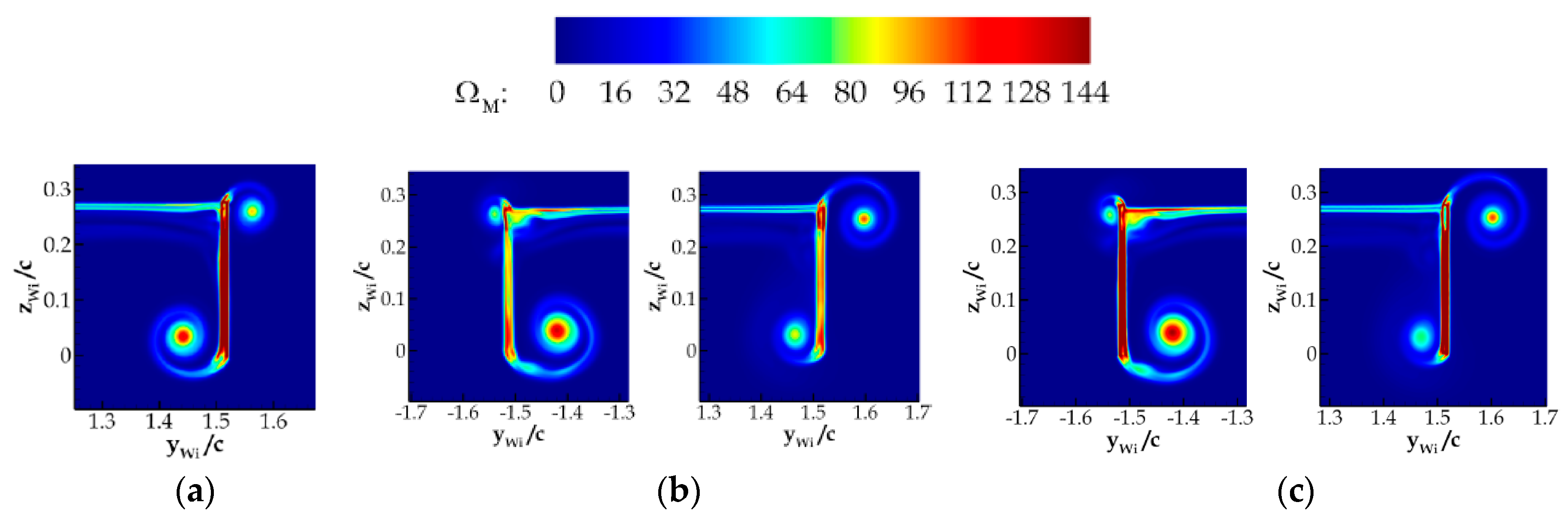
One of the largest alterations relative to the straight-line condition involves the comparative strengths of vortices within the trailing vortex system, particularly those shed from the endplates. In general, Vortex A and E are strengthened whilst the opposite occurs regarding Vortex B and D under the cornering or fixed yaw condition; this is quantified by Table 3 with a pictorial representation shown by Figure 27.
Comparing the cornering condition against the fixed yaw condition shows that the magnitude of strengthening or weakening of each vortex differ significantly. This is a combination of the effects of the freestream total pressure and the yaw angle variation present in the cornering condition; both of which are fixed for the yaw case. For example, Vortex E is strengthened to a larger degree under the yaw condition compared to the cornering condition despite the greater local yaw angle under the latter condition due to the reduced freestream total pressure.
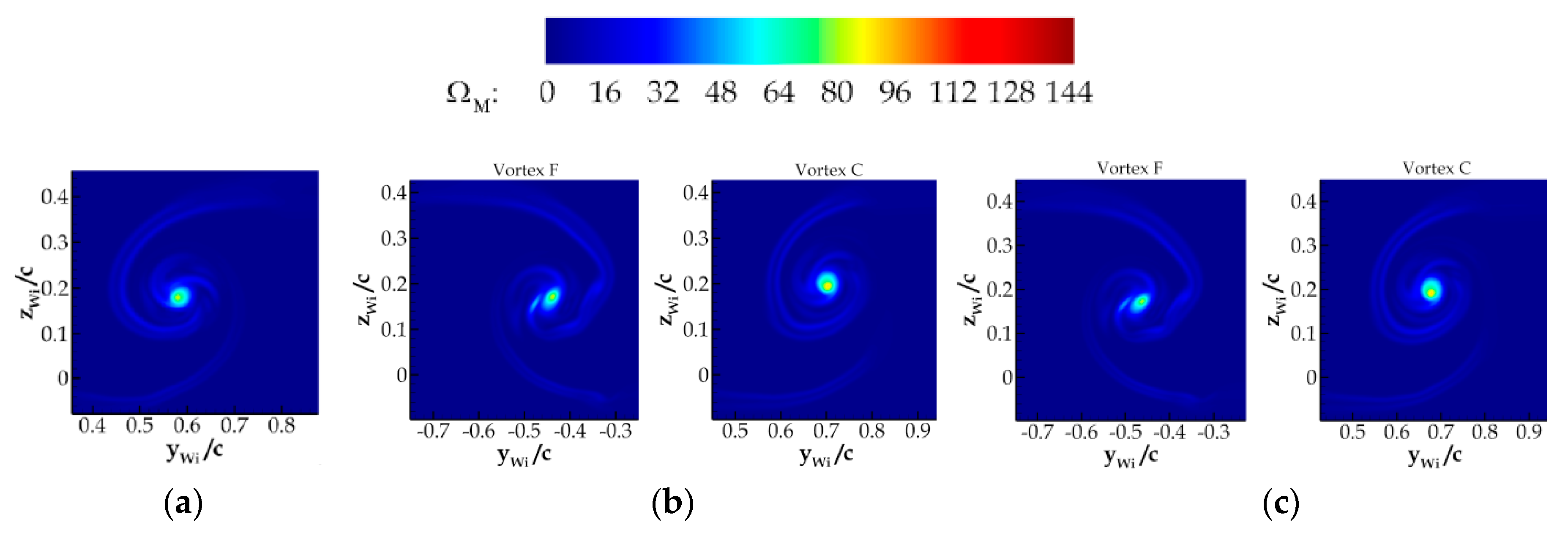
Vortex C and F are also significantly affected regarding their strength. Under the cornering condition, Vortex C is strengthened whilst Vortex F is weakened (Figure 28 and Table 4), with the relative strengthening of Vortex C being much greater than the weakening of Vortex F. The fixed yaw condition results in the strengthening of both Vortex C and F.
The size of a vortex involves a strong relationship with its strength as well as whether it has experienced any vortex merger. To elaborate, Vortex B was 52% larger in core diameter than Vortex A and 30% larger than Vortex C; the boundary of the core being defined as ΩM = 50. Interestingly, therefore, Vortex C consists of a larger core than Vortex A despite being weaker. This demonstrates one of the effects of vortex merging as noted in the existing literature [28,29]. Ultimately, it is found that the faster the vortex’s swirl rate, the larger the vortex core which may be further increased via vortex merger. This finding is unaltered under the cornering and fixed yaw angle conditions.
Whilst the location of the endplate vortices is largely unaffected by the cornering or fixed yaw conditions, the inboard tip vortices are greatly influenced by the direction of the freestream flow. Vortex F is located to be significantly closer to the centreline of the wing; at xWi/c = 1.624, by approximately 19% and 24% under the cornering and fixed yaw conditions respectively relative to the straight-line condition. Conversely, Vortex C is positioned further away from the centreline; at xWi/c = 1.624, by approximately 16% and 21% under the cornering and fixed yaw conditions respectively. The vertical positioning of the inboard tip vortices is also observed to differ where Vortex C is located consistently further away from the ground relative to Vortex F. In comparison to the straight-line condition, at xWi/c = 1.624, Vortex C is positioned approximately 6% further away from the ground whilst Vortex F is positioned approximately 6% closer the ground regarding the cornering condition. Under the fixed yaw condition, Vortex C is positioned approximately 7% further away from the ground whilst Vortex F is positioned approximately 6% closer to the ground.
4.4.3. Downstream Behaviour
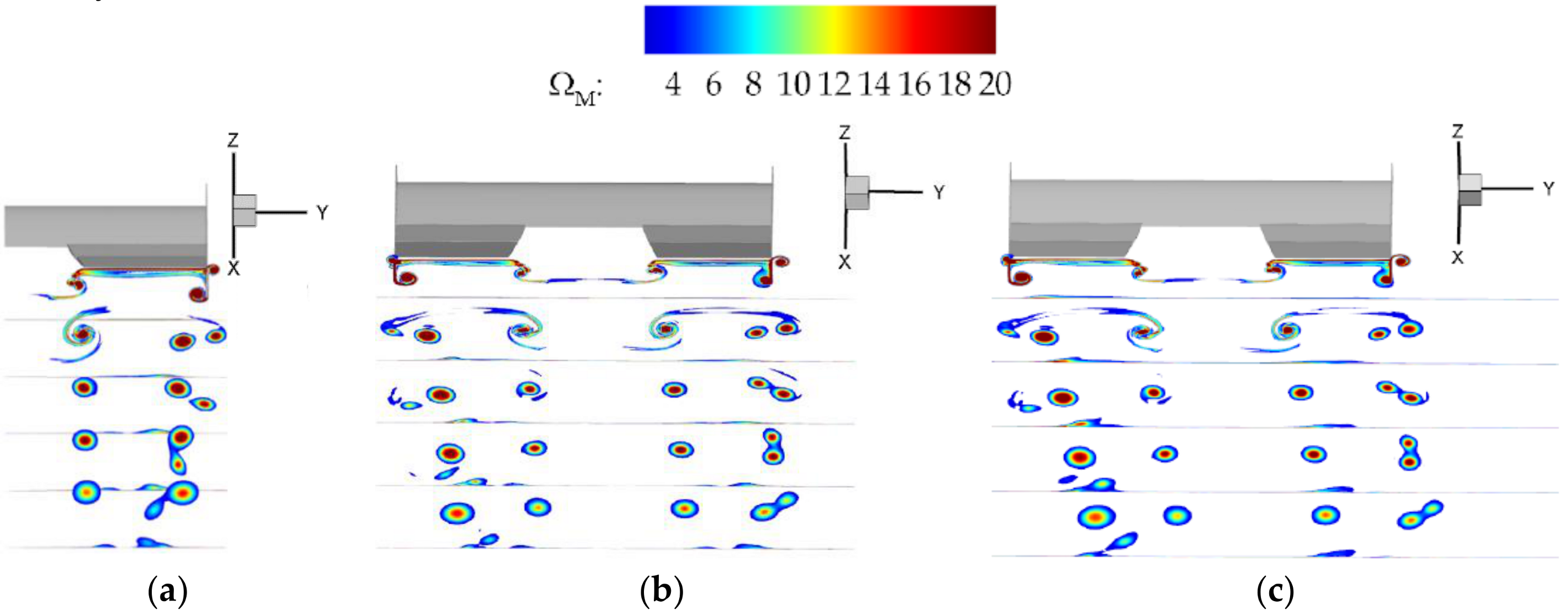
The downstream behaviour of the trailing vortex system under the straight-line condition, (Figure 29a), consists of three prominent features. These are the co-rotating vortex merger of Vortex A and Vortex B, the formation of a ground boundary layer and its consequent effects and the counter-rotating vortex interaction between Vortex C and the other vortices within the system.
Beginning with the downstream behaviour of Vortex A and Vortex B, these two co-rotating vortices are observed to eventually merge to form a single, coherent vortex. The merging process follows closely that described by Meunier et al. [28] and Cerretelli et al. [29] where both vortices initially rotate about each other. Within the critical separation distance, the weaker Vortex A is wrapped around Vortex B as described by Trieling et al. [26] whilst simultaneously transmitting its vorticity to the latter until it ceases to exist.
Focusing on the development of a ground boundary layer, as per Harvey et al.’s [30] observation, a ground boundary layer is formed due to the proximity of the vortices; this leads to the formation of a secondary vortex in some cases. It is believed that the existence of the secondary vortex is governed by a combination of the primary vortex consisting of sufficient strength and being positioned close enough to the ground. As Vortex A swings directly below Vortex B during the merging process, the development of the secondary vortex is accelerated.
Discussing the counter-rotating vortex interaction between Vortex C and the other vortices within the trailing vortex system, it is observed that the trailing vortex system features an upwards trajectory, most noticeably Vortex C. This behaviour is explained by considering each vortex as a point and treating Vortex C and the other vortices as a system of counter-rotating vortices of unequal strength. By applying the theory stated by Leweke et al. [31] and Batchelor [32], Vortex C is elevated as it is the weaker vortex.
Under the cornering and fixed yaw conditions, the downstream behaviour is affected in two main ways relative to the straight-line condition. This first is the path of the trailing vortex system and the second is downstream distance that is required for vortex merger to complete for the appropriate vortices.
Concerning the vortex trajectories, the path of each vortex, aside from the influence of the interaction with the other vortices, consists of a trajectory that follows the freestream flow. This, therefore, leads to the vortex system to be displaced outboards relative to the position of the wing with this behaviour augmented under fixed yaw relative to the cornering condition. This is particularly noticeable for the tip vortices C and F. This highlights the potential advantages of including true cornering in simulations if considering the interaction of vortices with downstream elements.
For both yaw and cornering, Vortex D and Vortex E merge within a significantly shorter downstream distance whilst Vortex A and Vortex B requires a greater distance in comparison to the straight-line condition. This is due to the differential in strength between the vortices in the vortex pair such that the greater the differential, the shorter the distance required to complete merger.
5. Conclusions
In this work we have used an SST Detached Eddy Simulation approach to investigate the changes to the aerodynamic performance of a representative race car front wing when cornering. The methodology has been validated against experimental work also presented in this paper. The simulations were seen to be in very good agreement with the experiment for forces and the off-surface velocity field. The simulation and experiment both revealed a trailing vortex system consisting of vortices produced at the top and bottom of the end plates and vortices produced at the tips of the part span flaps. The validated methodology was then applied to a direct comparison of straight-line and cornering conditions as well as a case at a fixed yaw angle based on the local yaw of the datum point of the cornering case. The latter represents what can be done in wind tunnel testing. The downforce was reduced slightly and the drag (defined as resistance to local freestream velocity) increased by around 5% as well as a side force (defined as force normal to local freestream) was also produced. This was due to the combined effects of both a variable local yaw and a higher freestream velocity at the outboard tip leading to modifications to the surface pressure distribution. The downstream trajectory of the vortex system was seen to be significantly altered between the straight line and cornering cases.
The fixed yaw case showed some differences to the surface pressure distribution from the cornering case although it was broadly similar. When defined in the original body axis the drag and side force differed from both straight line and cornering conditions. But when resolved into directions aligned with and normal to the wind direction a close agreement was seen between cornering and yaw cases. This suggests that if careful consideration is given to achieving an appropriate yaw angle then a fixed yaw test can give representative data for cornering performance of an isolated wing. However, the subsequent downstream trajectory of the vortex system was seen to be different for the cornering and yaw cases with the vortices being carried further outboard in the yaw case. Due to this care should be taken if attempting to investigate the interaction of multiple components on a vehicle using a fixed yaw test.
Author Contributions
Conceptualization, D.P., A.G. and M.P.; methodology, D.P.; software, D.P.; validation, D.P.; formal analysis, D.P.; investigation, D.P.; data curation, D.P.; writing—original draft preparation, D.P.; writing—review and editing, D.P., A.G. and M.P.; visualization, D.P.; supervision, A.G. and M.P.; project administration, A.G. and M.P. All authors have read and agreed to the published version of the manuscript.
Funding
This research was funded by both Loughborough University and the Engineering and Physical Sciences Research Council (EPSRC). We acknowledge the use of Athena at HPC Midlands+, which was funded by the EPSRC on grant EP/P 020232/1.
Acknowledgments
Both Max Varney and Andrew Horsey must be acknowledged for the technical support provided for the experimental part of this work.
Conflicts of Interest
The authors declare no conflict of interest. The funders had no role in the design of the study; in the collection, analyses, or interpretation of data; in the writing of the manuscript, or in the decision to publish the results”.
References
- Toet, W. Aerodynamics and aerodynamic research in Formula 1. Aeronaut. J. 2013, 117, 1–26. [Google Scholar] [CrossRef]
- Zerihan, J.; Zhang, X. Aerodynamics of a Single Element Wing in Ground Effect. J. Aircr. 2000, 37, 1058–1064. [Google Scholar] [CrossRef]
- Ranzenbach, R.; Barlow, J.B. Two-Dimensional Airfoil in Ground Effect, An Experimental and Computational Study. SAE Tech. Pap. Ser. 1994, 942509. [Google Scholar] [CrossRef]
- Agathangelou, B.; Gascoyne, M. Aerodynamic Design Considerations of a Formula 1 Racing Car. SAE Tech. Pap. Ser. 1998, 980399. [Google Scholar] [CrossRef]
- Zhang, X.; Toet, W.; Zerihan, J. Ground Effect Aerodynamics of Race Cars. Appl. Mech. Rev. 2006, 59, 33–49. [Google Scholar] [CrossRef] [Green Version]
- Wright, P.; Matthews, T. Formula 1 Technology. In Formula 1 Technology; SAE International: Warrendale, PA, USA, 2001. [Google Scholar]
- Keogh, J.; Doig, G.; Barber, T.; Diasinos, S. The Aerodynamics of a Cornering Inverted Wing in Ground Effect. Appl. Mech. Mater. 2014, 553, 205–210. [Google Scholar] [CrossRef] [Green Version]
- Keogh, J.; Doig, G.; Diasinos, S.; Barber, T. The influence of cornering on the vortical wake structures of an inverted wing. Proc. Inst. Mech. Eng. Part D: J. Automob. Eng. 2015, 229, 1817–1829. [Google Scholar] [CrossRef] [Green Version]
- Zhang, X.; Zerihan, J. Aerodynamics of a Double-Element Wing in Ground Effect. AIAA J. 2003, 41, 1007–1016. [Google Scholar] [CrossRef] [Green Version]
- Ranzenbach, R.; Barlow, J. Cambered Airfoil in Ground Effect—An Experimental and Computational Study. SAE Tech. Pap. Ser. 1996, 960909. [Google Scholar] [CrossRef]
- Marshall, D.; Newman, S.; Williams, C. Boundary layer effects on a wing in ground-effect. Aircr. Eng. Aerosp. Technol. 2010, 82, 99–106. [Google Scholar] [CrossRef]
- Zhang, X.; Zerihan, J. Off-Surface Aerodynamic Measurements of a Wing in Ground Effect. J. Aircr. 2003, 40, 716–725. [Google Scholar] [CrossRef]
- Soso, M.; Wilson, P.A. Investigating Changes to the Downforce Curve of a Double Element Airfoil in Ground Effect. SAE Tech. Pap. Ser. 2004. [Google Scholar] [CrossRef]
- 7th International symposium on applications of laser techniques to fluid mechanics. Int. J. Multiph. Flow 1994, 20. [CrossRef]
- Zhang, X.; Zerihan, J. Edge Vortices of a Double Element Wing in Ground Effect. J. Aircr. 2004, 41, 1127–1137. [Google Scholar] [CrossRef]
- Roberts, L.S.; Finnis, M.V.; Knowles, K.; Correia, J. Aerodynamic characteristics of a wing-and-flap configuration in ground effect and yaw. Proc. Inst. Mech. Eng. Part D: J. Automob. Eng. 2015, 230, 841–854. [Google Scholar] [CrossRef]
- Johl, G.S. The Design and Performance of a 1.9 m × 1.3 m Indraft Wind Tunnel. Ph.D. Thesis, Loughborough University, Loughborough, UK, 2010. [Google Scholar]
- Newnham, P.S. The Influence of Turbulence on the Aerodynamic Optimisation of Bluff Body Road Vehicles. Ph.D. Thesis, Loughborough University, Loughborough, UK, 2007. [Google Scholar]
- Siemens STAR-CCM+. User Guide V13.02; Siemens: Munich, Germany, 2018. [Google Scholar]
- Keogh, J.; Barber, T.J.; Diasinos, S.; Doig, G. Techniques for Aerodynamic Analysis of Cornering Vehicles. SAE Tech. Pap. Ser. 2015. [Google Scholar] [CrossRef]
- Wilson, J. Will a Moving Reference Frame (MRF) approach give a time-accurate flow solution? Siemens STAR-CCM+ Steve Portal 2018. Article No. 22106. [Google Scholar]
- Keogh, J. The Aerodynamic Effects of the Cornering Flow Conditions. Ph.D. Thesis, The University of New South Wales, Sidney, Australia, 2016. [Google Scholar]
- Josefsson, E.; Hagvall, R.; Urquhart, M.; Sebben, S. Numerical Analysis of Aerodynamic Impact on Passenger Vehicles during Cornering. SAE Tech. Pap. Ser. 2018. [Google Scholar] [CrossRef] [Green Version]
- Smith, A.M.O. High-Lift Aerodynamics. J. Aircr. 1975, 12, 501–530. [Google Scholar] [CrossRef] [Green Version]
- Van den Berg, M.A. Aerodynamic Interaction between a Inverted Wing with a Rotating Wheel. Ph.D. Thesis, University of Southampton, Faculty of Engineering and Applied Science, School of Engineering Sciences, Southampton, UK, 2007. [Google Scholar]
- Trieling, R.R.; Fuentes, O.U.V.; Van Heijst, G.J.F. Interaction of two unequal corotating vortices. Phys. Fluids 2005, 17, 87103. [Google Scholar] [CrossRef] [Green Version]
- Delery, J.M. Aspects of vortex breakdown. Prog. Aerosp. Sci. 1994, 30, 1–59. [Google Scholar] [CrossRef]
- Meunier, P.; Le Dizès, S.; Leweke, T. Physics of vortex merging. Comptes Rendus Phys. 2005, 6, 431–450. [Google Scholar] [CrossRef] [Green Version]
- Ceretelli, C.; Williamson, C.H.K. The physical mechanism for vortex merging. J. Fluid Mech. 2003, 475, 41–47. [Google Scholar] [CrossRef]
- Harvey, J.K.; Perry, F.J. Flowfield produced by trailing vortices in the vicinity of the ground. AIAA J. 1971, 9, 1659–1660. [Google Scholar] [CrossRef]
- Leweke, T.; Le Dizès, S.; Williamson, C.H. Dynamics and Instabilities of Vortex Pairs. Annu. Rev. Fluid Mech. 2016, 48, 507–541. [Google Scholar] [CrossRef] [Green Version]
- Batchelor, G.K. An Introduction to Fluid Dynamics; Cambridge University Press: Cambridge, UK, 2000. [Google Scholar]
Figure 1.
An image of the experimental setup. (a) Wing geometry; (b) False floor.

Figure 2.
Schematic diagram illustrating the datum point of the wing geometry i.e., xWi/c = 0, yWi/c = 0 and zWi/c = 0.
Figure 2.
Schematic diagram illustrating the datum point of the wing geometry i.e., xWi/c = 0, yWi/c = 0 and zWi/c = 0.

Figure 3.
PIV setup used to capture cross-plane velocity data.

Figure 4.
A schematic diagram showing an isometric view of the computational domains. (a) Numerical validation variant; (b) Full-scale simulation variant.
Figure 4.
A schematic diagram showing an isometric view of the computational domains. (a) Numerical validation variant; (b) Full-scale simulation variant.

Figure 5.
An illustration of the final mesh obtained from the mesh sensitivity study. (a) ywi/c = 1.11; (b) ywi/c = 1.76.
Figure 5.
An illustration of the final mesh obtained from the mesh sensitivity study. (a) ywi/c = 1.11; (b) ywi/c = 1.76.

Figure 6.
Contour showing the IDDES blending function at xWi/ce = 0.648; when the function = 0, LES is used, when the function = 1, RANS is used.
Figure 6.
Contour showing the IDDES blending function at xWi/ce = 0.648; when the function = 0, LES is used, when the function = 1, RANS is used.

Figure 7.
The boundary conditions applied for the straight-line condition. (a) Numerical validation variant; (b) Full-scale straight- line variant.
Figure 7.
The boundary conditions applied for the straight-line condition. (a) Numerical validation variant; (b) Full-scale straight- line variant.

Figure 8.
The boundary conditions for the cornering condition.

Figure 9.
The boundary conditions for the fixed yaw condition where φ represents the yaw angle.

Figure 10.
A schematic diagram showing the direction of the force vectors with respect to the wing under the straight-line and yaw conditions.
Figure 10.
A schematic diagram showing the direction of the force vectors with respect to the wing under the straight-line and yaw conditions.

Figure 11.
A schematic diagram showing the direction of the drag force and side-force vectors under the cornering condition; dWi denotes the absolute distance between the centre of pressure and the GCoR.
Figure 11.
A schematic diagram showing the direction of the drag force and side-force vectors under the cornering condition; dWi denotes the absolute distance between the centre of pressure and the GCoR.

Figure 12.
A schematic diagram defining the yaw angle of a particular cell.

Figure 13.
Contours showing a comparison of the mean vorticity magnitude of the endplate vortices at xWi/ce = 1.056. (a) Experiment (Unrepresentative reflection-induced vorticity visible near top endplate vortex); (b) Numerical solution.
Figure 13.
Contours showing a comparison of the mean vorticity magnitude of the endplate vortices at xWi/ce = 1.056. (a) Experiment (Unrepresentative reflection-induced vorticity visible near top endplate vortex); (b) Numerical solution.

Figure 14.
Contours showing a comparison of the mean vorticity magnitude of the inboard flap tip vortex at xWi/ce = 1.019. (a) Experiment; (b) Numerical solution.
Figure 14.
Contours showing a comparison of the mean vorticity magnitude of the inboard flap tip vortex at xWi/ce = 1.019. (a) Experiment; (b) Numerical solution.

Figure 15.
Contours showing the mean vorticity magnitude at several transverse locations ranging from xWi/ce = 1.204 and xWi/ce = 3.796. (a) Experiment; (b) Numerical solution.
Figure 15.
Contours showing the mean vorticity magnitude at several transverse locations ranging from xWi/ce = 1.204 and xWi/ce = 3.796. (a) Experiment; (b) Numerical solution.

Figure 16.
Graph showing the vorticity magnitude of the inboard tip vortex with downstream distance; curves are fitted to a 4th order polynomial.
Figure 16.
Graph showing the vorticity magnitude of the inboard tip vortex with downstream distance; curves are fitted to a 4th order polynomial.

Figure 17.
Contour showing the freestream yaw angle distribution on the surfaces under the cornering condition.
Figure 17.
Contour showing the freestream yaw angle distribution on the surfaces under the cornering condition.

Figure 18.
Contour showing the freestream velocity distribution on the wing under the cornering condition.
Figure 18.
Contour showing the freestream velocity distribution on the wing under the cornering condition.

Figure 19.
Contours showing the mean pressure coefficient distribution on the pressure surfaces. The stagnation pressure coefficient is 1 at the inboard and outboard region for the cornering condition; this is because it is calculated on a single reference velocity coinciding with that assigned at the LCoR. (a) Straight-line Condition; (b) Cornering condition; (c) Fixed yaw condition.

Figure 20.
Contours showing the mean pressure coefficient distribution on the pressure surfaces. (a) Straight-line Condition; (b) Cornering condition; (c) Fixed yaw condition.
Figure 20.
Contours showing the mean pressure coefficient distribution on the pressure surfaces. (a) Straight-line Condition; (b) Cornering condition; (c) Fixed yaw condition.

Figure 21.
Contours showing the mean of the total pressure loss at xWi/c = 1.019; the contour range has been capped to a maximum of 100% to improve the visibility of the wake. (a) Straight-line condition; (b) Cornering condition; (c) Fixed yaw condition.
Figure 21.
Contours showing the mean of the total pressure loss at xWi/c = 1.019; the contour range has been capped to a maximum of 100% to improve the visibility of the wake. (a) Straight-line condition; (b) Cornering condition; (c) Fixed yaw condition.

Figure 22.
Contours showing the mean of the total pressure loss at xWi/c = 2.545; the contour range has been capped to a maximum of 100% to improve the visibility of the wake. (a) Straight-line condition; (b) Cornering condition; (c) Fixed yaw condition.
Figure 22.
Contours showing the mean of the total pressure loss at xWi/c = 2.545; the contour range has been capped to a maximum of 100% to improve the visibility of the wake. (a) Straight-line condition; (b) Cornering condition; (c) Fixed yaw condition.

Figure 23.
A schematic diagram showing the trailing vortex system.

Figure 24.
Contours showing the mean vorticity magnitude at several transverse locations ranging from xWi/c = 0.0189 to xWi/c = 1 under the straight-line condition. (a) Formation of Vortex A; (b) Formation of Vortex B.
Figure 24.
Contours showing the mean vorticity magnitude at several transverse locations ranging from xWi/c = 0.0189 to xWi/c = 1 under the straight-line condition. (a) Formation of Vortex A; (b) Formation of Vortex B.

Figure 25.
Contour showing the mean vorticity magnitude at several transverse locations ranging from xWi/c = 0.0189 and xWi/c = 1.019 along the inboard endplate under the cornering condition.
Figure 25.
Contour showing the mean vorticity magnitude at several transverse locations ranging from xWi/c = 0.0189 and xWi/c = 1.019 along the inboard endplate under the cornering condition.

Figure 26.
Contours showing the mean vorticity magnitude at several transverse locations ranging from xWi/c = 0.507 and xWi/c = 1.624 under the straight-line condition.
Figure 26.
Contours showing the mean vorticity magnitude at several transverse locations ranging from xWi/c = 0.507 and xWi/c = 1.624 under the straight-line condition.

Figure 27.
Contours showing the mean vorticity magnitude of the endplate vortices at xWi/c = 1.019. (a) Straight-line condition; (b) Cornering condition; (c) Fixed yaw condition.
Figure 27.
Contours showing the mean vorticity magnitude of the endplate vortices at xWi/c = 1.019. (a) Straight-line condition; (b) Cornering condition; (c) Fixed yaw condition.

Figure 28.
Contours showing the mean vorticity magnitude of Vortex C at xWi/c = 1.624. (a) Straight-line condition; (b) Cornering condition; (c) Fixed yaw condition.
Figure 28.
Contours showing the mean vorticity magnitude of Vortex C at xWi/c = 1.624. (a) Straight-line condition; (b) Cornering condition; (c) Fixed yaw condition.

Figure 29.
Contours showing the mean vorticity magnitude at several transverse locations ranging from xWi/c = 1.019 and xWi/c = 3.704; the colour contour limits have significantly been decreased compared to previous figures to aid visualization. (a) Straight-line condition (b) Cornering condition; (c) Fixed yaw condition.


Table 1.
A table showing the lift and drag areas as well as the efficiency values obtained under the two evaluation methods.
Table 1.
A table showing the lift and drag areas as well as the efficiency values obtained under the two evaluation methods.
| Evaluation Method | CLWiA (m2) | CDWiA (m2) | |CLWiA|/CDWiA |
|---|---|---|---|
| Numerical | −0.169 | 0.026 | 6.500 |
| Experimental | −0.164 | 0.027 | 6.074 |
Table 2.
A table showing the lift, drag and side-force areas as well as the efficiency values obtained under all three conditions.
Table 2.
A table showing the lift, drag and side-force areas as well as the efficiency values obtained under all three conditions.
| Operating Condition | CLWiA (m2) | CDWiA (m2) | CSWiA (m2) | |CLWiA|/CDWiA |
|---|---|---|---|---|
| Straight-line | −0.808 | 0.100 | - | 8.080 |
| Cornering | −0.805 | 0.105 | 0.030 | 7.667 |
| Fixed Yaw | −0.804 | 0.099 | 0.045 | 8.121 |
| Fixed Yaw (WA) | −0.804 | 0.105 | 0.029 | 7.657 |
Table 3.
A table showing the change in strength of the endplate vortices at xWi/c = 1.019 under the cornering and fixed yaw conditions relative to the straight-line condition.
Table 3.
A table showing the change in strength of the endplate vortices at xWi/c = 1.019 under the cornering and fixed yaw conditions relative to the straight-line condition.
| Operating Condition | Vortex A | Vortex B | Vortex D | Vortex E |
|---|---|---|---|---|
| Cornering | +16% | −34% | −13% | +5% |
| Fixed Yaw | +17% | −43% | −9% | +12% |
Table 4.
A table showing the change in strength of the inboard flap tip vortices at xWi/c = 1.624 under the cornering and fixed yaw conditions relative to the straight-line condition.
Table 4.
A table showing the change in strength of the inboard flap tip vortices at xWi/c = 1.624 under the cornering and fixed yaw conditions relative to the straight-line condition.
| Operating Condition | Vortex C | Vortex F |
|---|---|---|
| Cornering | +11% | −2% |
| Fixed Yaw | +10% | +1% |
Publisher’s Note: MDPI stays neutral with regard to jurisdictional claims in published maps and institutional affiliations. |
© 2020 by the authors. Licensee MDPI, Basel, Switzerland. This article is an open access article distributed under the terms and conditions of the Creative Commons Attribution (CC BY) license (http://creativecommons.org/licenses/by/4.0/).
Share and Cite
MDPI and ACS Style
Patel, D.; Garmory, A.; Passmore, M. The Effect of Cornering on the Aerodynamics of a Multi-Element Wing in Ground Effect. Fluids 2021, 6, 3. https://0-doi-org.brum.beds.ac.uk/10.3390/fluids6010003
AMA Style
Patel D, Garmory A, Passmore M. The Effect of Cornering on the Aerodynamics of a Multi-Element Wing in Ground Effect. Fluids. 2021; 6(1):3. https://0-doi-org.brum.beds.ac.uk/10.3390/fluids6010003
Chicago/Turabian StylePatel, Dipesh, Andrew Garmory, and Martin Passmore. 2021. "The Effect of Cornering on the Aerodynamics of a Multi-Element Wing in Ground Effect" Fluids 6, no. 1: 3. https://0-doi-org.brum.beds.ac.uk/10.3390/fluids6010003