The Zoo of Modes of Convection in Liquids Vibrated along the Direction of the Temperature Gradient


Department of Mechanical and Aerospace Engineering, University of Strathclyde, James Weir Building, 75 Montrose Street, Glasgow G1 1XJ, UK
*
Author to whom correspondence should be addressed.
Fluids 2021, 6(1), 30; https://0-doi-org.brum.beds.ac.uk/10.3390/fluids6010030
Submission received: 9 December 2020
/
Revised: 2 January 2021
/
Accepted: 5 January 2021
/
Published: 8 January 2021
(This article belongs to the Special Issue Thermal Flows)
Abstract
:Thermovibrational flow can be seen as a variant of standard thermogravitational convection where steady gravity is replaced by a time-periodic acceleration. As in the parent phenomena, this type of thermal flow is extremely sensitive to the relative directions of the acceleration and the prevailing temperature gradient. Starting from the realization that the overwhelming majority of research has focused on circumstances where the directions of vibrations and of the imposed temperature difference are perpendicular, we concentrate on the companion case in which they are parallel. The increased complexity of this situation essentially stems from the properties that are inherited from the corresponding case with steady gravity, i.e., the standard Rayleigh–Bénard convection. The need to overcome a threshold to induce convection from an initial quiescent state, together with the opposite tendency of acceleration to damp fluid motion when its sign is reversed, causes a variety of possible solutions that can display synchronous, non-synchronous, time-periodic, and multi-frequency responses. Assuming a square cavity as a reference case and a fluid with Pr = 15, we tackle the problem in a numerical framework based on the solution of the governing time-dependent and non-linear equations considering different amplitudes and frequencies of the applied vibrations. The corresponding vibrational Rayleigh number spans the interval from Raω = 104 to Raω = 106. It is shown that a kaleidoscope of possible variants exist whose nature and variety calls for the simultaneous analysis of their temporal and spatial behavior, thermofluid-dynamic (TFD) distortions, and the Nusselt number, in synergy with existing theories on the effect of periodic accelerations on fluid systems.

1. Introduction
The direction of the prevailing temperature gradient is known to be an essential factor determining the properties of many distinct forms of thermal convection. This concept applies to both the stability scenario (i.e., the hierarchy of bifurcations undergone by the considered system when the applied temperature difference is increased) and the related patterning behavior. Archetypal situations for which the response of fluid systems to the application of an imposed temperature difference has been widely explored in the past are the cases where the thermal gradient is parallel or perpendicular to a fundamental reference direction typical of the considered problem.
For standard thermogravitational flow, i.e., fluid convection induced by buoyancy effects in non-thermally homogeneous fluids, this “reference direction” is obviously represented by gravity. Two fundamental conditions have enjoyed widespread attention over the years, leading to a true dichotomy in the literature, i.e., the cases where the angle Θ between the temperature gradient and gravity is either 0° or 90°. The former circumstance corresponds to the paradigm of Rayleigh–Bénard (RB) convection (namely fluid motion in a domain uniformly heated from below and cooled from above), the latter (originally studied by Hadley [1]) can be technically realized considering systems laterally bounded by vertical walls kept at different constant temperatures.
This rigid classification can also be found in companion problems where gravity is replaced by surface-tension effects (that is the case of fluid systems with a free surface, i.e., an interface where a liquid is in contact with another immiscible fluid). Fluid flow takes a different nomenclature according to the angle formed by the prevailing temperature gradient and the free interface. In particular, Θ = 0° and 90° correspond to the so-called thermocapillary and Marangoni–Bénard (MB) convection types, respectively.
Interestingly, buoyancy and surface-tension driven convection share more than a simple similarity in the related nomenclature. For both cases, a certain temperature difference (ΔT) must be exceeded before convection is produced when the temperature gradient is vertical (i.e., a “critical” ΔT exists), whereas fluid starts to move immediately (regardless of the effective magnitude of ΔT) when this gradient is horizontal.
However, while Marangoni–Bénard convection has been investigated essentially in infinite layers or domains uniformly heated from below with large horizontal extension, for Rayleigh–Bénard convection, a significant number of studies have been appearing where insights have been sought from consideration of the simplified setting corresponding to a square cavity. This configuration has enjoyed a widespread attention over the years owing to its simplicity and the concurrent possibility to produce flows that display or break the various intrinsic symmetries of this geometry (reflectional symmetries with respect to the vertical, horizontal, and diagonal directions). Moreover, it is known that if the Rayleigh number is increased beyond a certain critical threshold, the flow established inside the cavity can develop a complex sequence of instabilities (steady→time-periodic→low-dimensional chaos→fully turbulent states) even if fluid motion is forced to maintain a two-dimensional (2D) structure. Owing to space limitations, we do not strive to review the incredible amount of work existing on this subject. Mizushima [2] provided a complete characterization of the critical Rayleigh number for the onset of convection from the diffusive state considering convective disturbances with different possible symmetries. Mizushima and Adachi [3] concentrated on the ensuing non-linear regime, illustrating that the combination of fundamental modes that become critical for similar values of the Rayleigh number can result in different patterns. Relevant examples of typical dynamics can also be found in the numerical study by Goldhirsch et al. [4], where several complicated flow structures and textural transitions were observed together with multi-stability effects, i.e., the possibility to obtain different solutions (for a fixed geometry and boundary conditions) depending on the considered initial conditions.
For the turbulent regime, the reader is referred to the interesting theoretical works by Villermaux [5] and Kadanoff [6] and the more recent review (specifically devoted to the square cavity) by Lappa [7] (and all references therein).
Although the field of RB convection has reached a level of maturity, in the sense that various techniques are in position to address almost any question, we may ask regarding the various possible states or regimes for this type of flow—unfortunately, the companion problem where steady gravity is replaced by an acceleration changing periodically in time has not received considerable (similar) attention.
This flow is generally referred to as ‘thermovibrational convection’ because the most obvious (simplest) way to create an acceleration that varies sinusoidally in time is to apply vibrations to a fluid container. The average value of the acceleration produced in this way is zero, which explains why this form of convection is extremely relevant to the microgravity environment (conditions established onboard the International Space Station and other orbiting platforms), and it has recently enjoyed a remarkable resurgence in interest.
Similar to all the other types of thermal convection discussed before, also in this case, the angle between the imposed temperature gradient and the direction of the acceleration can have a remarkable impact on the emerging flow. In addition to the acceleration amplitude, the imposed ΔT, and the aforementioned angle Θ, an additional degree of freedom influencing the dynamics is represented by the ‘frequency’ of vibrations. Nevertheless, only a limited number of studies are available in the literature where this variant of buoyancy flow was considered (Monti et al. [8]; Alexander [9]; Alexander et al. [10,11]; Feonychev and Dolgikh [12]; Gershuni and Lyubimov [13]; Monti et al. [14]; Naumann [15]; Mialdun et al. [16]; Melnikov et al. [17]; Lyubimova et al. [18]; Bouarab et al. [19]; Shevtsova et al. [20,21]; Maryshev et al. [22]; Vorobev and Lyubimova [23]; Lappa, [24,25,26,27,28]; Lappa and Burel [29]). Still fewer articles have been devoted to the case where vibrations and temperature gradient are parallel. Moreover, most of them examined cases where vibrations were combined with steady gravity (modulated gravity), leading to results (see, e.g., Lappa [30] for an exhaustive review), which have limited translational relevance to pure thermovibrational convection.
To the best of our knowledge, only Hirata et al. [31] considered the pure thermovibrational flow in a square cavity assuming zero gravity and no inclination between vibrations and the temperature gradient. In the present study, an attempt is made to extend that earlier investigation to larger values of the Prandtl number and the Rayleigh number and elaborate a unified picture of the related hierarchy of instabilities and patterning behavior.
2. Mathematical Model
2.1. The Geometry
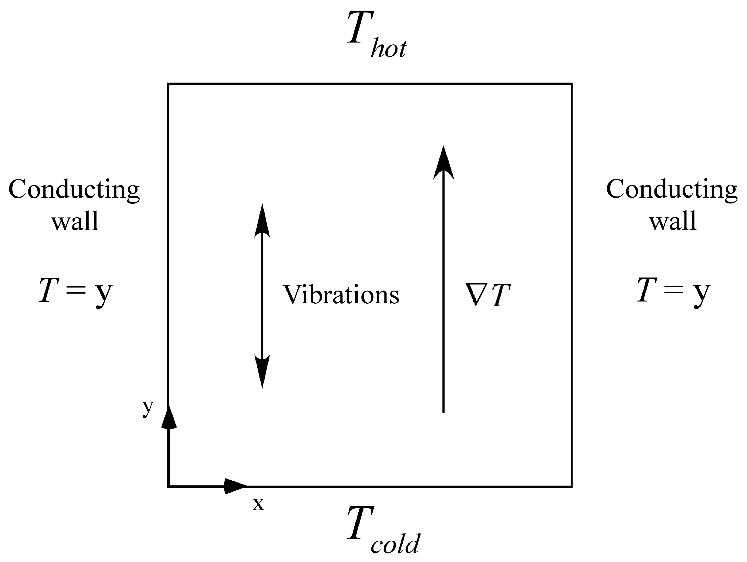
In keeping with a large portion of the work outlined in the introduction for standard RB convection, a simple 2D square cavity is considered. Microgravity conditions are assumed (no steady gravity). The direction of the temperature gradient and vibrations as well as the wall boundary conditions can be seen in Figure 1.
The buoyancy force responsible for fluid motion is produced by a sinusoidal displacement of the cavity with respect to time in addition to a temperature difference imposed along the same direction of shaking (along the y axis in Figure 1). The time periodic displacement (i.e., the vibrations) can be modeled mathematically as:
where b is the amplitude, ω = 2πf is the angular frequency of the displacement, and is the unit vector along the direction of vibrations. The ensuing time-varying acceleration can formally be obtained by taking the second derivative of Equation (1), which reads:
and satisfies the condition:
which shows that its time-averaged value over one period of oscillation 2π/ω is zero.
2.2. Balace Equations and Boundary Conditions
Using the Boussinesq approximation, and scaling the Cartesian coordinates (x,y), time (t), velocity (V), pressure (p), and temperature (T) by the reference quantities L, L2/α, α/L, ρα2/L2,and ΔT, respectively (where α is the fluid thermal diffusivity and ρ is the fluid density), the balance equations for mass, momentum, and energy can be cast in compact form as:
where:
and is the thermal expansion coefficient, ν is the fluid kinematic viscosity, and ΔT is the imposed temperature difference. As the reader will easily realize, Ω is the non-dimensional frequency of vibrations and might be seen as a variant of the classical Rayleigh number (based on the amplitude of the vibrations-induced acceleration bω2 in place of the standard gravity g).
Since in the present work, the vibrations and the imposed temperature gradient are both directed along the y axis, the projection of the momentum equation on the coordinate axes shown in Figure 1 reads:
where:
These equations must be integrated with the relevant initial and boundary conditions, which in the present work are set as follows:
i.e., quiescent conditions and linear temperature distribution along y at the initial instant (t = 0) and
i.e., no-slip conditions for all the solid walls, conducting thermal conditions for the walls parallel to imposed vibrations, and different constant temperatures on the perpendicular boundaries.
T = y and u = v = 0 for 0 ≤ x ≤ 1, 0 ≤ y ≤ 1 and t = 0
T = y and u = v = 0 for x = 0, x = 1, 0 ≤ y ≤ 1 and t > 0
T = 0 and u = v = 0 for y = 0, 0 ≤ x ≤ 1 and t > 0
T = 1 and u = v = 0 for y = 1, 0 ≤ x ≤ 1 and t > 0
2.3. Embedded Symmetries
Notably, following Mizushima [2], assembled in this way, these equations and the related boundary conditions allow meaningful “a priori” reflections about the possible symmetries of the emerging convective modes in a square cavity, which can be categorized as follows:
- (ss): The symmetric–symmetric mode. This mode is characterized by an even number of rolls along the two coordinate axes. It reduces to a configuration with the central symmetry if the same number (m) of rolls affects both the x and y directions, i.e., mx = my (whereas a columnar arrangement is obtained if my > mx).
- (sa): The symmetric–antisymmetric mode. This mode displays symmetry only with respect to the y-axis; accordingly, the flow typically features an odd number of rolls along y and an even number of rolls along the other axis.
- (as): The antisymmetric–symmetric mode. This mode displays symmetry only with respect to the x-axis; accordingly, the flow typically features an odd number of rolls along x and an even number of rolls along the other axis.
- (aa): The antisymmetric–antisymmetric mode. No symmetry is retained in this case, as the number of rolls is odd along both axes (a single column being obtained for my > mx = 1).
This classification, largely used in the past (see, e.g., Mizushima [2] and Mizushima and Adachi [3]) to interpret the typical patterning behavior of standard buoyancy convection in square cavities heated from below and cooled from above (Rayleigh–Bénard convection), will be applied in the present work to characterize the spatial properties of the emerging thermovibrational flow.
3. Numerical Method
The integration of Equations (4)–(6) in addition to the initial and boundary conditions allows for the unknown pressure (p), velocity (V), and temperature (T) fields to be found. The related procedure (time-marching algorithm) is described in the present section.
Along these lines, it is worth starting from the simple observation that, as implicitly made evident by the aforementioned set of equations, these three fundamental physical quantities (“primitive variables”) display a varying degree of interrelation, depending on the specific couple considered. As an example, while V and p are intimately linked through the momentum equation, the temperature field (T) can be determined once the velocity field is known through the energy equation (Equation (6)).
In particular, the link between the first two unknowns is at the root of the so-called class of projection or fractional methods (Harlow and Welch [32]; Chorin [33]; Temam [34]; Gresho and Sani [35]; Gresho [36]; Guermond and Quartapelle [37]; Guermond et al. [38]). These techniques rely on the so-called Hodge decomposition theorem, which states that any vector field can be decomposed into a divergence-free contribution and the gradient of a scalar potential (a curl-free part). Stripped to its essentials, the related computational scheme can synthetically be described as follows. Initially, the pressure is artificially neglected in the balance of momentum in order to obtain an equation (Equation (18)) where only the velocity field requires solving for:
In this way, even though the pressure is initially unknown, a time-marching procedure can be started. However, the field V* obtained through integration of this equation is called ‘provisional’ because, obviously, it does not account for the impact of pressure on fluid flow; moreover, it does not satisfy the incompressibility constraint (represented by the separate equation for the balance of mass). Nevertheless, using the aforementioned Hodge decomposition theorem, V* can formally be split into two contributions as follows:
where V and ∇p play the role of divergence-free vector and the gradient of a scalar potential, respectively. This step is purely formal, as p is one of the unknowns. The next conceptual ingredient needed to obtain a complete time-marching procedure that consists of forcing V = V*−C∇p into Equation (4). In this way, indeed, a ‘working’ equation for the effective determination of the pressure is obtained:
V*= V+ C∇p
This equation represents the ‘core’ of all variants pertaining to the aforementioned class of projection (or fractional) methods. After Equation (18) has been integrated, the pressure can be determined solving Equation (20); finally, the sought divergence-free velocity field can be computed from Equation (19) as V = V*−C∇p (assuming C = Δt where Δt is the time integration step).
The well-posedness of this approach is guaranteed by another important fundamental theorem—that is, the so-called theorem of the inverse calculus (see, e.g., Ladyzhenskaya [39]); it states that a vector field is uniquely determined when its divergence and curl are assigned; in the present case, these are and , where the latter equality follows from the well-known mathematical property of the curl operator to annihilate the gradient of a scalar function, i.e., (Gresho [36]; Lappa [40]; Lappa and Boaro [41]).
In the present work, we have used the specific variant of this class of methods available in the OpenFOAM computational platform (OpenCFD Ltd 2019, London, UK), i.e., the so-called PISO (Pressure Implicit Split Operator) approach (originally elaborated by Issa [42]). The OpenFOAM implementation of this method relies on a collocated grid approach, which means that the unknowns are defined in the center of the computational cells. Moreover, in order to improve the coupling of velocity and pressure, a special interpolation of the velocity is applied on the cell faces (Rhie and Chow [43]), while the third unknown T is determined in a segregated manner after the computation of V and p. Finally, we wish to remark that we have used backward differencing in time and upwind differencing schemes in space for both the convective term and diffusion term, while the solution of Equation (20) has been based on a Generalized Geometric-Algebraic Multi-Grid (GAMG) strategy.
4. Validation
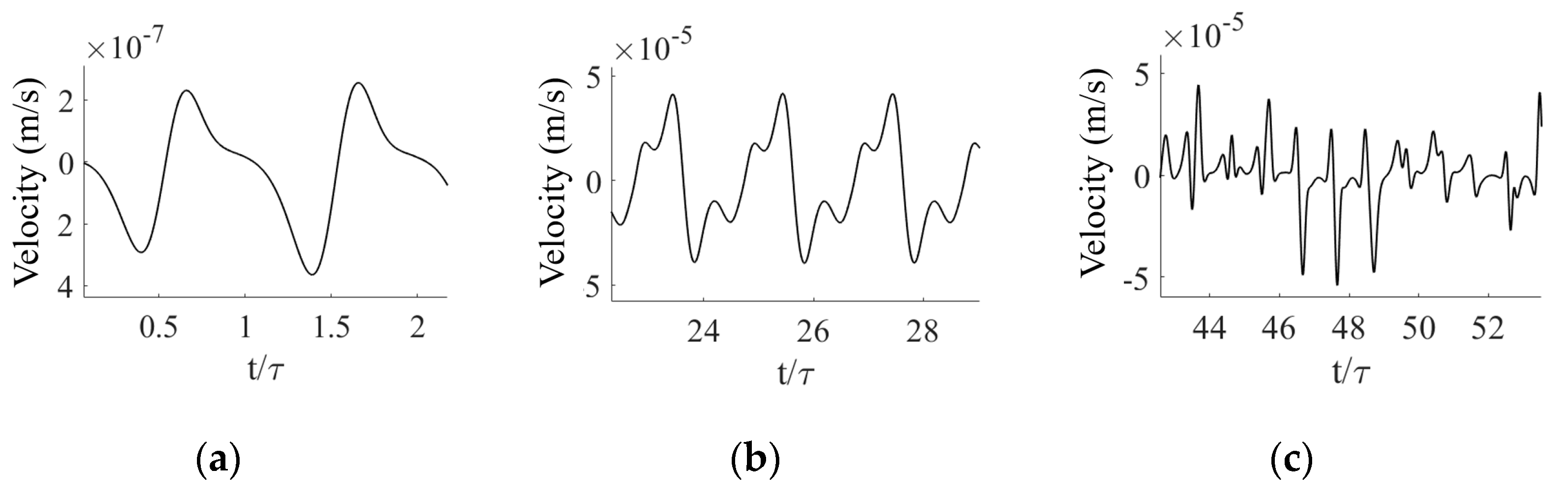
Before numerical results can be interpreted, it is imperative that the strategy for the solution of the governing equations is validated against available relevant benchmarks. Given our specific target, the earlier study by Hirata et al. [31] is specifically considered for such a purpose. In particular, three cases are chosen: (a) Ω = 200, = 7 × 10⁴, (b) Ω = 500, = 105, and (c) Ω = 200, = 105 (the velocity signals for these cases are readily available to the reader in the original study, making the comparison with the current results straightforward). As the reader will realize by inspecting Figure 2, the present results are in excellent agreement with the original signals reported by Hirata et al. [31], both in shape and periodicity.
For the sake of completeness, additional validation has been obtained considering quantitative comparison with other well-known benchmarks in the literature concerned with classical RB convection in a square cavity ([44,45]). These comparisons have already been published in Lappa and Inam [46] and are not duplicated here for the sake of brevity.
5. Grid Refinement Study
Due to the potential complexity of the flow considered in this study, close attention must also be given to the grid adopted for the numerical simulations. Although mesh refinement criteria for thermovibrational flow are not available, meaningful indications in this regard can be obtained through ‘analogies’ with parent forms of convection. As an example, relevant similarities with standard gravitational convection in high-Pr fluids include the development of thermal boundary layers for relatively high values of the Rayleigh number. For the case of standard buoyancy flow, as an example, Russo and Napolitano [47] showed that a working correlation for the thickness of the thermal boundary layer can be introduced as follows:
The presence of such boundary layers cannot be ignored when designing an adequate mesh and can be translated into precise numerical requirements. As an example, relevant information along these lines can be found in the study on RB convection by Shishkina et al. [48], where the number of cells required in the thermal boundary layer has been specified directly as a function of Ra, i.e.,
Another important influential factor to be taken into account (especially when one targets high-Ra regimes) in the preliminary definition of a computational grid is the so-called Kolmogorov length scale, i.e., the need to keep the size of the computational cell sufficiently small to capture the ‘eddies’ that are produced when the flow assumes a turbulent behavior. It is known that for standard RB convection (De et al. [49]), this characteristic (non-dimensional) length scales as
All these criteria should be regarded as a set of multiple requirements finally leading to a relevant mesh. Assuming the worst conditions considered in the present work, i.e., the highest possible value of , all these constraints taken together would return a uniform mesh 102 × 102.
To verify the consistency of this way of thinking with the standard approach generally used to define a suitable mesh (i.e., a ‘classical grid refinement study’), we have increased progressively the number of computational nodes until convergence has been obtained. The outcomes of such a study are presented in Figure 3, where the maximum of the difference between the instantaneous temperature and the corresponding time-averaged (over the period of vibrations) value has been plotted (the so-called thermofluid-dynamic distortion). It can be seen that the results for a grid of size 82 × 82 are extremely close to that of the grid size 102 × 102, which implicitly indicates that (toward the end to save computational time) one may limit to considering the former coarser mesh. However, in order to meet all the possible criteria described before (see Table 1), we have decided to use the 102 × 102 mesh for all the cases considered in the present work.
As an additional layer of validation, comparisons with an in-house explicit code have also been made (this is presented a posteriori in Section 6.2, where the same mesh resolution of 102 × 102 is used).
6. Results
With the numerical approach robustly tested by (1) verifying its ability to capture available results in the literature and (2) checking its convergence under mesh refinement (forcing the used grids to also satisfy existing practical and theoretical criteria about mesh design), we have then simulated a vast range of cases by varying parametrically the vibrational Rayleigh number and the frequency of vibrations over three orders of magnitude. In particular, the same value of the Prandtl number originally considered by Lappa [7] has been examined (Pr = 15) with the two-fold purpose of (1) extending that earlier study conducted for classical RB convection in a square cavity to the case of thermovibrational flow and (2) expanding the space of parameters originally examined by Hirata et al. [31]. In order to consider conditions for which the flow can still be considered laminar or weakly chaotic (the investigation of the fully turbulent regime being beyond the scope of the present work), the maximum value of the Rayleigh number has been limited to 106.
The work/study progresses with the aid and support of both global parameters and detailed velocity fields for a better representation of the emerging dynamics. While a coarse-grained macroscopic perspective is used at the beginning by providing results in terms of maps (Section 6.1 and Section 6.2) and general trends in terms of ‘distortions’ (Section 6.3) and Nusselt number (Section 6.4), the problem is considered from a fine-grained micromechanical level in Section 6.5 (in terms of flow temporal behavior and related symmetries). We finally link (Section 7) the resulting statistics to the evolution of global parameters to provide useful information about the underlying cause-and-effect relationships.
6.1. Regime Classification
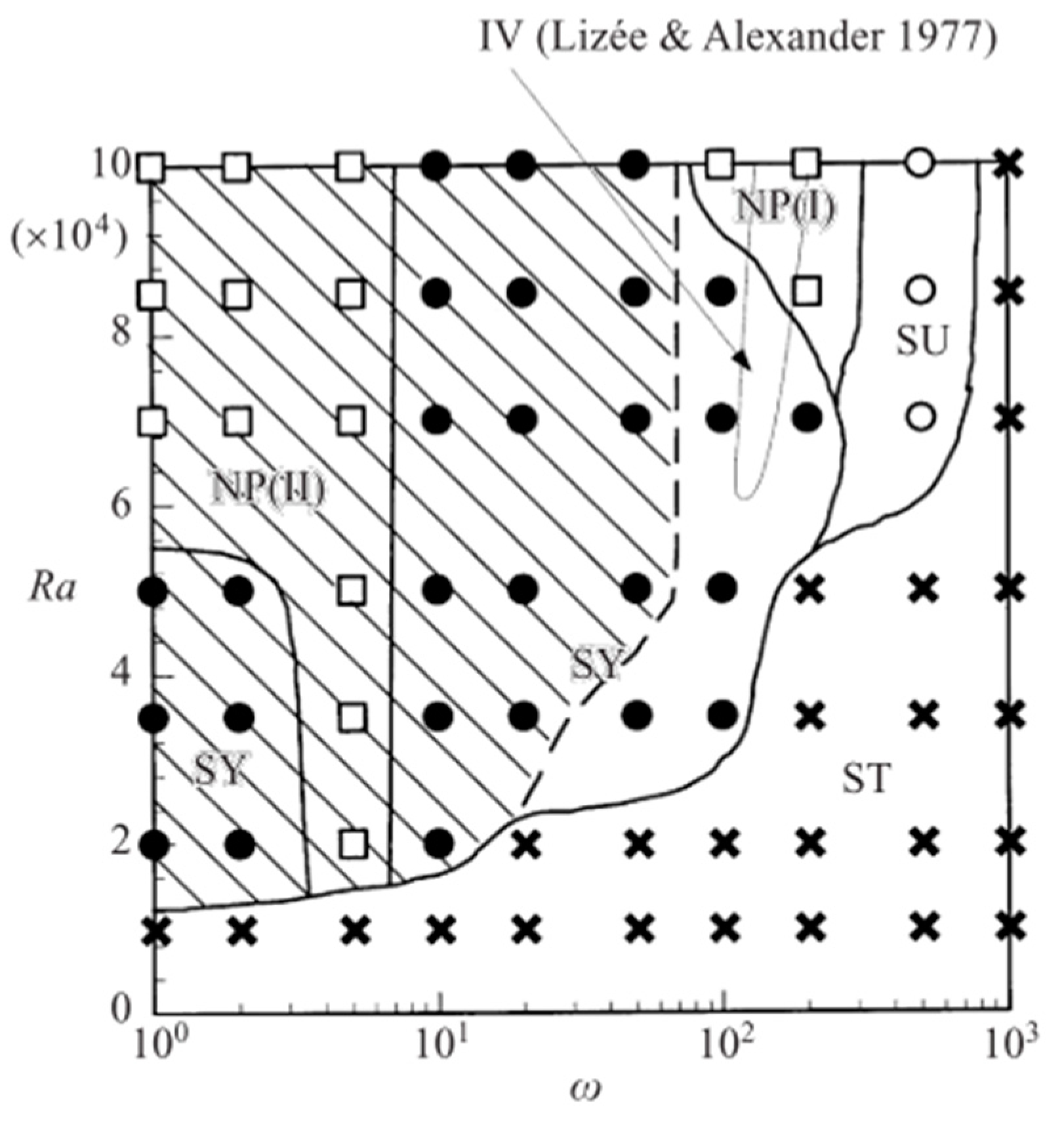
As the present study has been expressly conceived as an extension of the numerical investigation originally conducted by Hirata et al. [31], the simplest way to place the present results in an adequate context is to start from an overview of that work (see Figure 4).
The diversity of flow regimes that exist for pure thermovibrational convection in a square cavity when the temperature gradient is imposed parallel to the vibration can be clearly seen in this figure. Hirata et al. [31] split these regimes into four possible categories, namely, Synchronous (SY), Subharmonic (SU), Non-periodic (NP), and Stable (ST) solutions. Unfortunately, these authors limited themselves to considering values of the vibrational Rayleigh number in the range (104 ≤ ≤ 105, the constraint on the upper value being essentially an outcome of the limited computational resources available at that time). This figure is instructive also for another reason. It shows the well-known stabilization of thermovibrational flow when the frequency of vibrations is increased (Simonenko and Zen’kovskaja [50]; Simonenko [51]; Gershuni and Zhukhovitskii [52]; Gershuni et al. [53]; Gershuni and Zhukhovitskii [54]); we will come back to this fundamental concept later.
A total of 66 new simulations have been conducted in the present work. In line with Hirata et al. [31], Ω has been varied from Ω = 1 to Ω = 103, with the addition of a very high value of Ω = 104. As explained before, a fluid with Pr = 15 has been considered in place of Pr = 7. Another distinguishing mark of the present analysis is the extension to = 106.
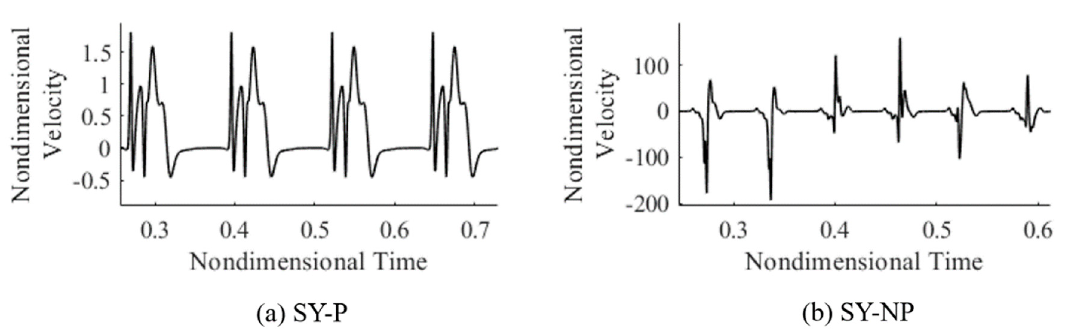
Before starting to deal with the detailed discussion of these results, we wish to anticipate that although the regimes (SY, SU, NP, and ST) were sufficient to compartmentalize the flow in the range of parameters considered by Hirata et al. [31], additional classes of flow have been identified for the cases simulated here in the interval (105 < < 106). These new findings have implicitly led to the need to introduce a distinction within the synchronous regime whereby a flow may be synchronous and periodic or synchronous and non-periodic (SY-P or SY-NP). Relevant examples of such new solutions are shown in Figure 5a,b, respectively. In particular, Figure 5a relates to the circumstances where the velocity signal is identical over each period for all periods (therefore, the signal can be considered synchronous and periodic). By contrast, although the signal shown in Figure 5b is still synchronous in time with the applied forcing (i.e., the vibrations), it also exhibits turbulent busts every period; moreover, the signal is not periodic, as the bursts display a more or less erratic evolution in time.
6.2. Map Extension
The main outcome of the present parametric investigation, i.e., the extended map, is presented in Figure 6. It is divided into regions where clusters of convective modes can be observed. Although stabilization is achieved at extremely high frequencies (Ω = 104), the predominant flow regime apparent for high vibrational Rayleigh numbers ( > 5 × 10⁵) is the aforementioned SY-NP case denoted by ![Fluids 06 00030 i010]() . The red sinusoidal signal included in the insets represents the forcing applied to the system; it is instrumental in making evident that the turbulent bursts for the SY-NP mode occur synchronously with the forcing but do not display the same behavior for each period. These solutions are less ordered than those found for the lower vibrational Rayleigh numbers whereby they appear in less organized clusters. The appearance of the SY-P regime is more sporadic. However, this mode of convection also exists at extremely high Rayleigh numbers ( = 106), which indicates that an increase in does not systematically lead to a more chaotic system (in some regions of parameters (Ω = 103), the flow reverts from an NS-NP back to an SY-P state).
. The red sinusoidal signal included in the insets represents the forcing applied to the system; it is instrumental in making evident that the turbulent bursts for the SY-NP mode occur synchronously with the forcing but do not display the same behavior for each period. These solutions are less ordered than those found for the lower vibrational Rayleigh numbers whereby they appear in less organized clusters. The appearance of the SY-P regime is more sporadic. However, this mode of convection also exists at extremely high Rayleigh numbers ( = 106), which indicates that an increase in does not systematically lead to a more chaotic system (in some regions of parameters (Ω = 103), the flow reverts from an NS-NP back to an SY-P state).
 . The red sinusoidal signal included in the insets represents the forcing applied to the system; it is instrumental in making evident that the turbulent bursts for the SY-NP mode occur synchronously with the forcing but do not display the same behavior for each period. These solutions are less ordered than those found for the lower vibrational Rayleigh numbers whereby they appear in less organized clusters. The appearance of the SY-P regime is more sporadic. However, this mode of convection also exists at extremely high Rayleigh numbers ( = 106), which indicates that an increase in does not systematically lead to a more chaotic system (in some regions of parameters (Ω = 103), the flow reverts from an NS-NP back to an SY-P state).
 In agreement with Hirata et al. [31], in the range of low frequencies Ω < 200, the fluid displays a stationary behavior over a certain sub-interval of the period τ (= 2π/Ω) of the applied vibrations.
In addition to enlightening the reader on the complexity and unpredictability of the flow regime (with the exception of extremely high values of Ω for which the dynamics reduce to the emergence of a quiescent thermally diffusive state), this map provides a picturesque description of the velocity signals and the fluid behavior.
The thermal response of the system is described in the next section where some dedicated (‘ad hoc’) definitions and concepts are introduced.
However, before starting to deal with thermal effects, we wish to remark that an extra layer of validation (with respect to that illustrated in Section 4) has been implemented comparing the results obtained here for the new cases (using OpenFOAM) with those provided by the same code used by Lappa [25] and Lappa and Burel [29] (see Figure 7). Both OpenFOAM and this code pertain to the same class of pressure–velocity methods discussed before. However, while OpenFOAM is based on an implicit approach (for what concerns the time integration) and on a collocated distribution of unknowns, the computational platform used by Lappa [25] and Lappa and Burel [29] relies on an explicit approach and a ‘staggered’ arrangement of variables, respectively.
It can be seen that despite the differences highlighted above, the shape and periodicity of the signals produced by both codes are in agreement (the discrepancy in signal amplitude can be expected as the exact location of the probes and the positive direction of the axes of the reference Cartesian system differ from solver to solver).
6.3. Themofluid-Dynamic Disturbances
A further understanding of the observed dynamics can be gained through the so-called thermofluid-dynamic (TFD) distortions. These characteristic quantities have enjoyed a widespread use in past studies concerned with the effect of vibrations on non-isothermal fluid systems (see, e.g., Monti et al. [14]). They can be used to characterize in a synthetic way the thermal response of the fluid to the application of a time-varying acceleration.
However, a proper introduction of these characteristic quantities requires a short excursus on the peculiar properties of thermovibrational flows. In particular, it is worth recalling that a non-isothermal fluid subjected to vibrations can develop a stationary response in addition to the oscillatory velocity field directly induced by the time-periodic acceleration. The latter can easily be explained assuming a straightforward cause-and-effect relationship between the time-varying buoyancy force and the induced fluid motion. The former requires a more involved interpretation. This stationary response (detectable through analysis of the time-averaged flow field) is an outcome of the non-linear nature of the balance equations (Savino and Lappa [55]). It becomes significant when the frequency of vibrations is sufficiently high and their amplitude is relatively small, i.e., in the so-called Gershuni regime (Simonenko and Zen’kovskaja [50]; Simonenko [51]; Gershuni and Zhukhovitskii [52]; Gershuni et al. [53]; Gershuni and Zhukhovitskii [54]; Savino and Lappa [55]; Lappa [30]). Indeed, for the opposite circumstances for which the frequency is small and the amplitude large, the linear response (direct proportionality between the oscillatory flow and the time-dependent acceleration) is dominant [55]. The time-averaged and fluctuating components of the velocity and temperature fields can formally be defined as:
and
In the present work, these quantities have been determined “a posteriori” after evaluating V and T via direct numerical solution of the governing equations in their complete time-dependent and non-linear form, as illustrated in Section 3.
The above-mentioned distortions can be defined accordingly as follows:
where Tdiff represents the temperature field that would be established in the absence of convection (in other words, a purely diffusive temperature profile, which using the reference system indicated in Figure 1 would simply read Tdiff = y).
Taking into account that (as illustrated above) the local temperature can be split into a time-averaged steady component plus a fluctuating part , Equation (26) can be further expanded as:
where represents the companion averaged distortion, i.e.,
Global measures can be defined accordingly as:
.
TFD = max (δT) for 0 ≤ x ≤ 1, 0 ≤ y ≤ 1 to ≤ t ≤ to + τ (where τ=2π/Ω)
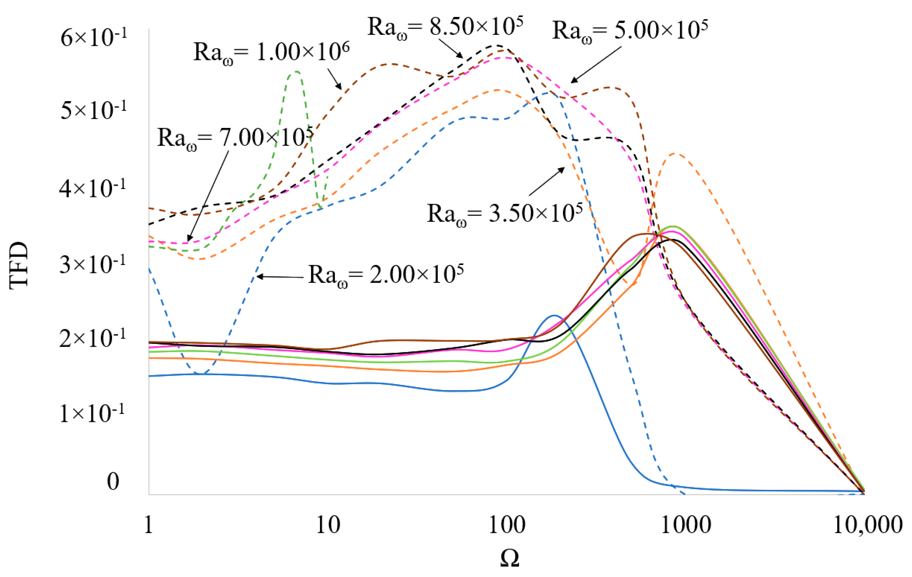
These quantities are reported in Figure 8 and Figure 9 for different circumstances (δT and represented by dashed and solid lines, respectively).
As quantitatively substantiated by these figures, the oscillatory thermofluid dynamic disturbance (TFD) is generally higher that the time-averaged one over the considered range of frequencies.
In particular, the time-averaged disturbances are approximately constant if their dependence on either or Ω is considered until the critical value of Ω = 500 is attained, where these disturbances are seen to increase (with the exception of the case = 2 × 10⁵ for which the TFDaveraged tends to 0).
For what concerns the oscillatory disturbances, an increase in TFD occurs until the critical value of Ω = 100, while for Ω > 100, the opposite trend can be seen.
Remarkably, all the TFD distortions tend to zero as the frequency grows. A simple way to think about this scenario is to consider that it reflects the existence of the almost quiescent states already reported in Figure 6. However, from a physical point of view, this trend can be interpreted directly, taking into account a well-known property of thermovibrational flow for high frequencies (for Ω ≥ 104, i.e., when the Gershuni regime is approached (Savino and Lappa [55]). As originally argued by Birikh at al. [56], indeed, in the limit as the frequency tends to infinite, if temperature distortions with respect to the purely diffusive case are present, the major role of the mean vibration force is that of forcing isotherms to turn and become perpendicular to the vibration direction. To elucidate further the significance of this observation, one should keep in mind that in other words, this simply means that an intrinsic property of thermovibrational convection induced by vibrations parallel to the imposed temperature difference is to tend naturally to a quiescent thermally diffusive state as Ω is increased (which provides the sought physical justification for the ST states reported in the existence map).
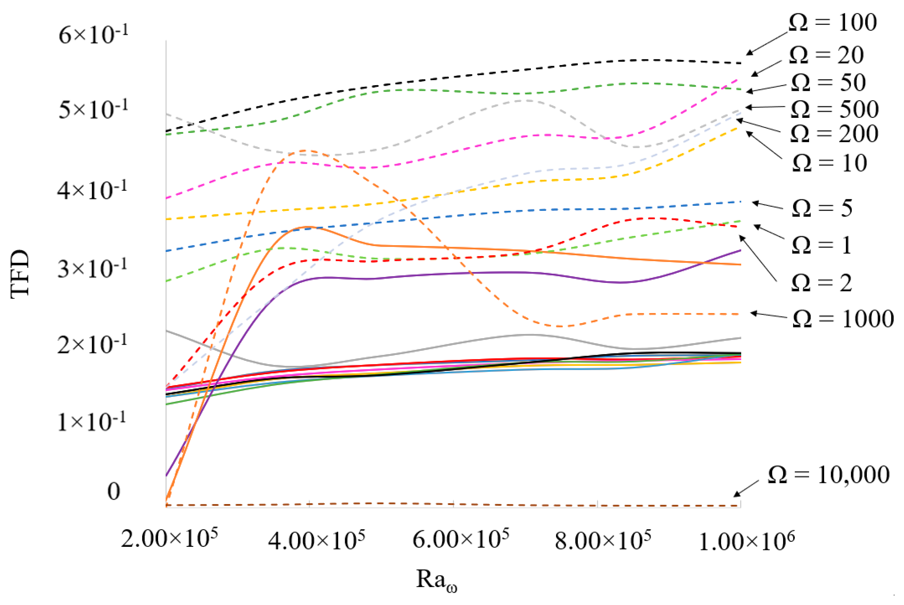
Apart from showing that the oscillatory disturbances prevail over the time averaged ones, Figure 8 and Figure 9 are also instrumental in revealing that the increase of the vibrational amplitude () affects the two types of distortions differently: as already explained to a certain extent before, the time-averaged disturbances seem quasi-independent of the increase in (or value of Ω in fact), whereas the instantaneous (complete) TFD are appreciably affected by both and Ω.
6.4. Evaluation of the Nusselt Number
In keeping with the previous section, further analysis of the thermal behavior of the system may be carried out by looking at another global parameter, i.e., the classical Nusselt number, namely the ratio of heat transfer due to convection over the heat transfer due to conduction along a given boundary. In our case, this non-dimensional number can be defined as:
and we introduce accordingly
Numax= max (Nu) for to ≤ t ≤ to + τ.
In the case of high frequencies, it has been shown in the previous section that when parallel to the temperature gradient, the vibrations have a stabilizing effect on the flow. This trend can still be appreciated when cases with > 105 and the SY-NP and NS-NP regimes are considered. As witnessed by Figure 10, a remarkable decrease in Numax occurs for Ω = 1000 (Numax ideally tending to 1 in the limit as Ω→∞). However, as still evident in this figure, a peak is located Ω = 100. For all values of at low frequencies (Ω < 20), Numax remains constant; then, it grows for intermediate frequencies (50 < Ω < 100) and finally decreases for high values of Ω (Ω > 1000).
However, upon increasing (as expected), Numax tends to become higher for all values of Ω (Figure 11).
Notably, the peak located at Ω ≅ 100 is consistent with the maximum taken by the TFD (see again Figure 8), and the key to understanding this finding lies in considering that, given the dominance of instantaneous effects on time-averaged ones, the effective configuration of the temperature field (in terms of topology of the isotherms and ensuing heat exchange at the boundaries) must essentially be ascribed to the fluctuating components of velocity and temperature. As already outlined above, the tendency of the Nusselt number toward the unit value as Ω is increased is indirect evidence of the fact that fluid motion tends to be suppressed in those conditions.
6.5. Streamlines and Patterning Behaviors
In this section, we finally concentrate on the effective patterning behavior of the flow for the different regimes reported in Figure 6. Emphasis is put on the interval 105 < ≤ 106, as these circumstances were not covered in the earlier study by Hirata et al. [31].
Along these lines, we begin from the case = 106, Ω = 104, i.e., a condition for which the flow is almost negligible (“stable state”). As shown by Figure 12, it manifests itself as an (ss) convective mode characterized by two rolls along each coordinate axis. This extremely weak flow starts as a four-roll configuration. From there, small rolls nucleate at the corners of the cavity and, as time passes, they tend to merge with their respective neighbors until the original quadrupolar arrangement is recovered. This nucleation occurs twice in the space of a period rapidly regaining the four-roll configuration. The periodicity of this evolutionary scenario is consistent with the velocity signal (which is sinusoidal and synchronous with the forcing period).
Another characteristic type of solution present in the map (Figure 6) is the synchronous and periodic state (SY-P). This mode of convection can be found mainly at the center and at the left side of the map for < 5 × 10⁵. As illustrated in Figure 13, this regime presents periodically identical instantaneous velocity fields and streamlines. In this case, the quadrupolar (four-roll) configuration is interrupted at each period by the genesis of two small rolls in the center of the lower part of the cavity, which are eventually flattened, hence allowing the flow to return to the original pattern.
The next figure of the sequence (Figure 14) illustrates a Subharmonic case (SU). In this figure, the typical behavior of a subharmonic mode of convection can be recognized in both the velocity field and streamlines snapshots. The period of the flow is double with respect to that of the forcing. However, the signature of the forcing period τ can still be recognized if one considers the two spikes (one large and one small) visible in the signal (then, these spikes are repeated with a slightly lower amplitude in the second forcing period). This is also quantitatively substantiated by the panels (a) and (b), where the magnitude of the first velocity field is (slightly) higher than that of the second.
In terms of spatial symmetry, the (aa) type is dominant (one single roll). However, during one period of flow oscillation, modes with the (ss) symmetry are excited, which combined with the main roll give rise to one diagonal clockwise-oriented vortex with two small counter-rotating eddies located in opposite corners of the cavity or a columnar arrangement of three superposed rolls slightly inclined to the left.
The next case serves to reveal the intrinsic features of the synchronous and non-periodic regime (SY-NP) found at higher vibrational Rayleigh numbers and at low and intermediate frequencies. As already explained in Section 6.1, a distinguishing mark of this type of solutions is the existence of bursts in the velocity signal, which display a more or less random nature.
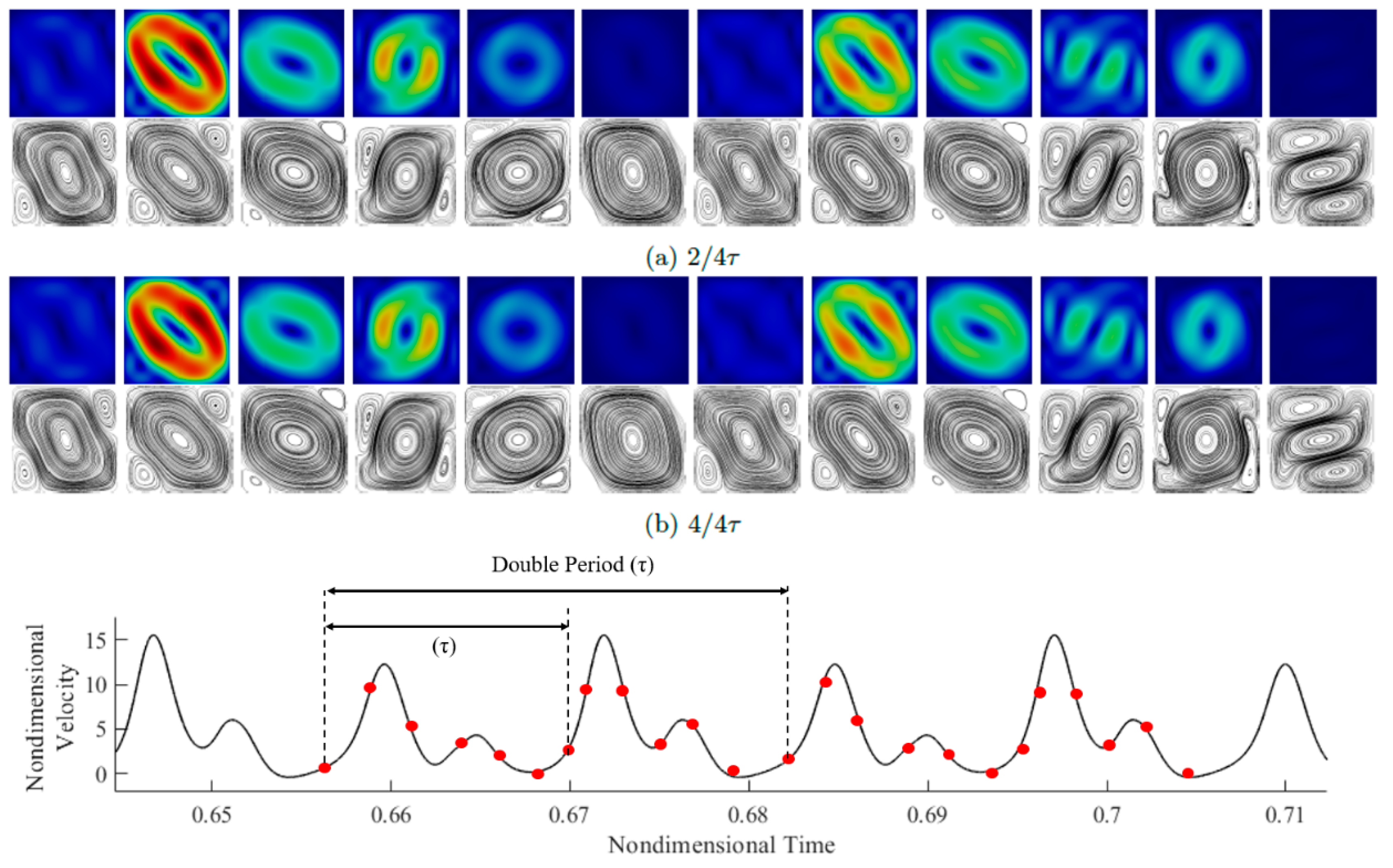
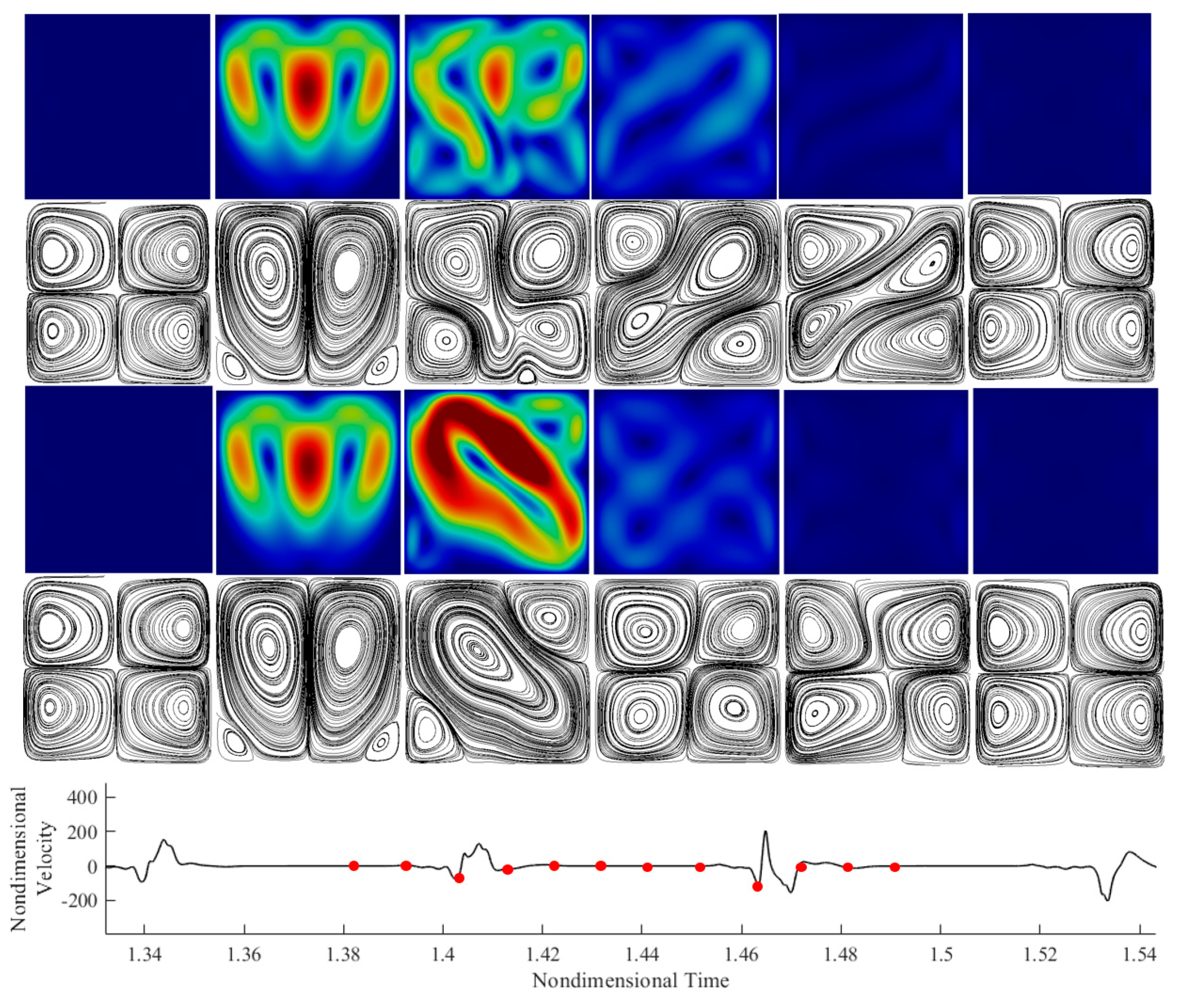
In particular, here, the case of = 8.5 × 10⁵, Ω = 100 is taken as a representative example (Figure 15). As a fleeting glimpse into this figure would immediately confirm, the fluid becomes almost quiescent over a fixed sub-interval of each period.
Although the velocity profile shows a large difference in behavior over time, the instantaneous velocity field and streamlines witness that the actual pattern is different at each turbulent burst. This is evident in the third, fourth, and fifth snapshots of the sequence for each period. Although the bust occurs at the same point in time, the flow structure changes considerably.
When the velocity magnitude is close to zero, the streamlines present again the four-roll configuration; when a burst occurs, as shown in snapshot 3, existing vortices merge, and new rolls appear randomly. In terms of spatial symmetry, although in certain sub-intervals of the period solutions with the (sa) symmetry also appear (two vertically extended rolls in a side-by-side configuration), the (ss) mode with four rolls is generally dominant.
Figure 16 can be finally used to get insights into the non-synchronous and non-periodic regime (NS-NP) apparent in the region of high vibrational frequencies. Easily identifiable, these solutions exhibit no adherence to the imposed vibrational forcing. As the reader will easily realize by inspecting Figure 16, the behavior of the flow changes randomly and presents a number of interesting and unpredictable topological (in terms of streamlines) features, which essentially result from the excitation and superposition of convective modes with different symmetries.
7. Discussion and Conclusions
Originally conceived as an extension of other works in the literature, the present study has confirmed that a kaleidoscope of solutions can be obtained in an apparently innocuous configuration such as a square cavity subjected to vibrations parallel to the applied temperature difference. Considering relatively high values (heretofore unexplored) of the vibrational Rayleigh number and non-dimensional angular frequency, two new states have been identified in the space of parameters, namely, periodic and non-periodic synchronous modes of convection. The peculiarity of the latter resides in its ability to produce turbulent bursts, which occur synchronously with the forcing but do not display the same behavior in each period of oscillation. Although the appearance of the synchronous periodic solution is more sporadic, this mode of convection can manifest itself also for high Rayleigh numbers, which indicates that an increase in does not systematically lead to more chaotic phenomena.
Comparison with equivalent studies conducted for the same value of the Prandtl number, same geometry, and same range of values of the Rayleigh number for classical Rayleigh–Bénard convection indicates that the set of potentially excitable modes with different symmetries is greatly expanded when the steady gravity is replaced by a time-periodic acceleration. From the limited series of snapshots included in the present work, the predominantly occurring symmetries are represented by the symmetric–symmetric mode (ss) (generally appearing as a quadrupolar pattern) and the diagonal mode characterized by a predominant central vortex ornated with two smaller outer corner rolls. However, occasional manifestations of other patterns are also possible, including (but not limited to) the vertical two-roll configuration (sa), the columnar arrangement of three horizontally stretched rolls, as well as other three-roll configurations. In line with earlier studies on the companion problem of standard RB convection, we argue that an explanation for this variety of multicellular states can be rooted in the existence of multiple solutions, i.e., different possible modes of convection that coexist in the space of parameters and can be excited for comparable values of the driving force (Mizushima [2]; Hof et al. [57]; Leong [58]; Lappa [59]). These modes are not mutually exclusive, nor are they truly progressive, which means that they can be excited at different times or at the same time, resulting in new patterns due to their non-linear combination.
A comparison of instantaneous and time-averaged effects also leads to meaningful conclusions. The former is generally dominant over the entire range of values of and Ω considered. The dependence on the problem parameters also displays notable differences. While time-averaged quantities are almost independent from the vibrational Rayleigh number, instantaneous ones grow (as expected) with this parameter. However, as the angular frequency of the imposed vibrations is increased, both fluctuating and time-averaged (stationary) effects (as properly quantified through the so-called TFD distortions) tend to be damped until a completely motionless state is attained (for a cut-off value of the frequency that grows with the considered value of ). This scenario is consistent with that revealed by the Nusselt number (which tends to 1 as this cut-off value is exceeded, thereby indicating that purely thermally diffusive conditions are established). It is also congruent with the so-called Birikh’s law, i.e., the expected tendency of the time-averaged vibration force to create isotherms perpendicular to the direction of vibrations when the frequency becomes relatively high (thereby causing a strong increase in the value of the Rayleigh number needed to produce convection, which ideally tends to infinite in the limit as Ω→∞, [60]).
The peak visible in both the instantaneous TFD and Nu plot at Ω ≅ 100 for relatively high values of the vibrational Rayleigh number calls for a complementary explanation. This can be further elaborated in its simplest form on the basis of the argument that the fluctuating components of velocity and temperature are dominant and therefore play a crucial role in determining the intensity of the heat exchange at the solid boundaries. Moreover, we argue that an explanation for the non-monotone behavior must be sought in the spatial symmetries of the dominant flow. Indeed, the specific value of the angular frequency for which the maximum is attained (Ω ≅ 100) in the range of high values of the vibrational Rayleigh number corresponds to conditions where the (ss) symmetry (multicellular state) is dominant (its reverberation on the heat exchange being an increase in magnitude).
Given the lack of studies specifically conceived to investigate the properties of pure thermovibrational flow in conditions for which the temperature gradient is parallel to the direction of shaking, this work has been conducted under the optimistic idea that it may provide a common point of origin from which many studies in the community may depart (including meaningful extensions to three-dimensional configurations). These future works might be based on the same variegated approach used in the present work, which has proven instrumental in unraveling processes that are interwoven or overshadowed and successful at illuminating the dynamical mechanisms at play on these systems, thereby making research results easier to compare and providing researchers with reasonable values to assume for areas outside their experience.
Author Contributions
Data curation, G.C.; Formal analysis, M.L.; Investigation, G.C. and M.L.; Methodology, M.L.; Software, G.C. and M.L.; Supervision, M.L.; Visualization, G.C.; Writing—original draft, G.C. and M.L.; Writing—review and editing, M.L. All authors have read and agreed to the published version of the manuscript.
Funding
This work has been supported by the UK Space Agency (grants ST/S006354/1 and ST/V005588/1) in the framework of the “particle vibration” (T-PAOLA) project.
Institutional Review Board Statement
Not applicable.
Informed Consent Statement
Informed consent was obtained from all subjects involved in the study.
Data Availability Statement
Publicly available datasets were analyzed in this study. These data can be found in the pure repository of the University of Strathclyde.
Conflicts of Interest
The authors declare no conflict of interest.
Nomenclature
| Nomenclature | |
| b | Vibration amplitude |
| Nu | Nusselt number |
| p | Pressure |
| Pr | Prandtl number |
| Ra | Rayleigh number |
| s | Displacement |
| T | Temperature |
| t | Time |
| u | Velocity component along x |
| V | Velocity |
| v | Velocity component along y |
| x | Horizontal coordinate |
| y | Vertical coordinate |
| Greek Symbols | |
| α | Thermal diffusivity |
| βT | Thermal expansion coefficient |
| ν | Kinematic viscosity |
| ρ | Fluid density |
| ω | Dimensional angular frequency |
| Ω | Non-dimensional angular frequency |
| ΔT | Temperature difference |
| τ | Non-dimensional period of vibrations |
| δ | Thickness |
| ζ | Kolmogorov length scale |
| Subscripts | |
| BL | Boundary layer |
| Cold | Cold |
| diff | Diffusive |
| Hot | Hot |
| max | Maximum |
| Superscripts | |
| Lab | Laboratory |
References
- Hadley, G. Concerning the cause of the general trade winds. Philos. Trans. R. Soc. Lond. 1735, 29, 58–62. [Google Scholar]
- Mizushima, J. Onset of thermal convection in a finite two–dimensional box. J. Phys. Soc. Jpn. 1995, 64, 2420–2432. [Google Scholar] [CrossRef]
- Mizushima, J.; Adachi, T. Sequential Transitions of the Thermal Convection in a Square Cavity. J. Phys. Soc. Jpn. 1997, 66, 79–90. [Google Scholar] [CrossRef]
- Goldhirsch, I.; Pelz, R.B.; Orszag, S.A. Numerical simulation of thermal convection in a two-dimensional finite box. J. Fluid Mech. 1989, 199, 1–28. [Google Scholar] [CrossRef]
- Villermaux. Memory-induced low frequency oscillations in closed convection boxes. Phys. Rev. Lett. 1995, 75, 4618–4621. [Google Scholar] [CrossRef]
- Kadanoff, L.P. Turbulent Heat Flow: Structures and Scaling. Physics Today 2001, 54, 34–39. [Google Scholar] [CrossRef]
- Lappa, M. Some considerations about the symmetry and evolution of chaotic Rayleigh–Bénard convection: The flywheel mechanism and the “wind” of turbulence. C. R. Mécanique 2011, 339, 563–572. [Google Scholar] [CrossRef]
- Monti, R.; Langbein, D.; Favier, J.J. Influence of residual accelerations on fluid physics and material science experiments. In Fluid and material Science in Space: A European Perspective; Walter, H.U., Ed.; Springer: Berlin, Germany, 1987; Chapter XVIII; pp. 637–680. [Google Scholar]
- Alexander, J.I.D. Low gravity experiment sensitivity to residual acceleration: A review. Microgravity Sci. Technol. 1990, 3, 52–68. [Google Scholar]
- Alexander, J.I.D.; Ouazzani, J.; Rosenberger, F. Analysis of the low gravity tolerance of Bridgman-Stockbarger crystal growth, II. Transient and periodic accelerations. J. Cryst. Growth 1991, 113, 21–38. [Google Scholar] [CrossRef]
- Alexander, J.I.D.; Garandet, J.-P.; Favier, J.J.; Lizee, A. g-jitter effects on segregation during directional solidification of tin-bismuth in the MEPHISTO furnace facility. J. Cryst. Growth 1997, 178, 657–661. [Google Scholar]
- Feonychev, A.I.; Dolgikh, G.A. Influence of vibration on heat and mass transfer in microgravity conditions. Microgravity Q. 1994, 4, 233–240. [Google Scholar]
- Gershuni, G.Z.; Lyubimov, D.V. Thermal Vibrational Convection; Wiley: Chichester, UK, 1998. [Google Scholar]
- Monti, R.; Savino, R.; Lappa, M. Microgravity sensitivity of typical fluid physics experiment. In Proceedings of the 17th Microgravity Measurements Group Meeting, Cleveland, OH, USA, 24–26 March 1998; Published in the Meeting Proceedings in NASA CP-1998-208414. pp. 1–15. [Google Scholar]
- Naumann, R.J. An analytical model for transport from quasi-steady and periodic accelerations on spacecraft. Int. J. Heat Mass Transf. 2000, 43, 2917–2930. [Google Scholar] [CrossRef]
- Mialdun, A.; Ryzhkov, I.I.; Melnikov, D.E.; Shevtsova, V. Experimental Evidence of Thermal Vibrational Convection in a Nonuniformly Heated Fluid in a Reduced Gravity Environment. Phys. Rev. Lett. 2008, 101, 084501. [Google Scholar] [CrossRef] [PubMed] [Green Version]
- Melnikov, D.; Ryzhkov, I.; Mialdun, A.; Shevtsova, V. Thermovibrational Convection in Microgravity: Preparation of a Parabolic Flight Experiment. Microgravity Sci. Technol. 2008, 20, 29–39. [Google Scholar] [CrossRef]
- Lyubimova, T.P.; Perminov, A.V.; Kazimardanov, M.G. Stability of quasi-equilibrium states and supercritical regimes of thermal vibrational convection of a Williamson fluid in zero gravity conditions. Int. J. Heat Mass Transf. 2019, 129, 406–414. [Google Scholar] [CrossRef]
- Bouarab, S.; Mokhtari, F.; Kaddeche, S.; Henry, D.; Botton, V.; Medelfef1, A. Theoretical and numerical study on high frequency vibrational convection: Influence of the vibration direction on the flow structure. Phys. Fluids 2019, 31, 043605. [Google Scholar] [CrossRef] [Green Version]
- Shevtsova, V.; Lyubimova, T.; Saghir, Z.; Melnikov, D.; Gaponenko, Y.; Sechenyh, V.; Legros, J.C.; Mialdun, A. IVIDIL: On-board g-jitters and diffusion controlled phenomena. J. Phys. Conf. Ser. 2011, 327, 012031. [Google Scholar] [CrossRef]
- Shevtsova, V.; Mialdun, A.; Melnikov, D.; Ryzhkov, I.; Gaponenko, Y.; Saghir, Z.; Lyubimova, T.; Legros, J.C. The IVIDIL experiment onboard the ISS: Thermodiffusion in the presence of controlled vibrations. C. R. Mécaniq 2011, 339, 310–317. [Google Scholar] [CrossRef]
- Maryshev, B.; Lyubimova, T.; Lyubimov, D. Two-dimensional thermal convection in porous enclosure subjected to the horizontal seepage and gravity modulation. Phys. Fluids 2013, 25, 084105. [Google Scholar] [CrossRef]
- Vorobev, A.; Lyubimova, T. Vibrational convection in a heterogeneous binary mixture. Part I. Time-averaged equations. J. Fluid Mech. 2019, 870, 543–562. [Google Scholar] [CrossRef] [Green Version]
- Lappa, M. Control of convection patterning and intensity in shallow cavities by harmonic vibrations. Microgravity Sci. Technol. 2016, 28, 29–39. [Google Scholar] [CrossRef] [Green Version]
- Lappa, M. The patterning behavior and accumulation of spherical particles in a vibrated non-isothermal liquid. Phys. Fluids 2014, 26, 093301. [Google Scholar] [CrossRef] [Green Version]
- Lappa, M. Numerical study into the morphology and formation mechanisms of threedimensional particle structures in vibrated cylindrical cavities with various heating conditions. Phys. Rev. Fluids 2016, 1, 25. [Google Scholar] [CrossRef] [Green Version]
- Lappa, M. On the multiplicity and symmetry of particle attractors in confined non-isothermal fluids subjected to inclined vibrations. Int. J. Multiphase Flow 2017, 93, 71–83. [Google Scholar] [CrossRef] [Green Version]
- Lappa, M. On the formation and morphology of coherent particulate structures in non-isothermal enclosures subjected to rotating g-jitters. Phys. Fluids 2019, 31, 11. [Google Scholar] [CrossRef] [Green Version]
- Lappa, M.; Burel, T. Symmetry Breaking Phenomena in Thermovibrationally Driven Particle Accumulation Structures. Phys. Fluids 2020, 32, 23. [Google Scholar] [CrossRef]
- Lappa, M. Thermal Convection: Patterns, Evolution and Stability; John Wiley & Sons, Ltd.: Chichester, UK, 2009. [Google Scholar]
- Hirata, K.; Sasaki, T.; Tanigawa, H. Vibrational effects on convection in a square cavity at zero gravity. J. Fluid Mech. 2001, 445, 327–344. [Google Scholar] [CrossRef]
- Harlow, F.H.; Welch, J.E. Numerical calculation of time-dependent viscous incompressible flow with free surface. Phys. Fluids 1965, 8, 2182–2189. [Google Scholar] [CrossRef]
- Chorin, A.J. Numerical solutions of the Navier-Stokes equations. Math. Comput. 1968, 22, 745–762. [Google Scholar] [CrossRef]
- Temam, R. Sur l’approximation de la solution des èquations de Navier-Stokes par la mèthode des pas fractionnaires (I). Arch. Rat. Mech. Anal. 1969, 33, 377–385. [Google Scholar] [CrossRef]
- Gresho, P.M.; Sani, R.T. On pressure boundary conditions for the incompressible Navier-Stokes equations. Int. J. Numer. Meth. Fluids 1987, 7, 1111–1145. [Google Scholar] [CrossRef]
- Gresho, P.M. Incompressible fluid dynamics: Some fundamental formulation issues. Ann. Rev. Fluid Mech. 1991, 23, 413–453. [Google Scholar] [CrossRef]
- Guermond, J.-L.; Quartapelle, L. On stability and convergence of projection methods based on pressure Poisson equation. Int. J. Numer. Meth. Fluids 1998, 26, 1039–1053. [Google Scholar] [CrossRef] [Green Version]
- Guermond, J.-L.; Minev, P.; Shen, J. An Overview of Projection Methods for Incompressible Flows. Comput. Methods. Comput. Methods Appl. Mech. Eng. 2006, 195, 6011–6045. [Google Scholar] [CrossRef] [Green Version]
- Ladyzhenskaya, O.A. The Mathematical Theory of Viscous Incompressible Flow, 2nd ed.; Gordon and Breach: New York, NY, USA; London, UK,, 1969. [Google Scholar]
- Lappa, M. Strategies for parallelizing the three-dimensional Navier-Stokes equations on the Cray T3E. In Science and Supercomputing at CINECA; Voli, M., Ed.; CINECA: Bologna, Italy, 1997; Volume 11, pp. 326–340. ISBN 10:88-86037-03-1. [Google Scholar]
- Lappa, M.; Boaro, A. Rayleigh-Bénard convection in viscoelastic liquid bridges. J. Fluid Mech. 2020, 904. [Google Scholar] [CrossRef]
- Issa, R.I. Solution of the implicitly discretized fluid flow equations by operator-splitting. J. Comp. Phys. 1986, 62, 40–65. [Google Scholar] [CrossRef]
- Rhie, C.M.; Chow, W.L. Numerical study of the turbulent flow past an airfoil with trailing edge separation. AIAA J. 1983, 21, 1525–1532. [Google Scholar] [CrossRef]
- Lappa, M.; Inam, S. Thermogravitational and hybrid convection in an obstructed compact cavity. Int. J. Thermal Sci. 2020, 156, 21. [Google Scholar] [CrossRef]
- Ouertatani, N.; Cheikh, N.B.; Beya, B.B.; Lili, T. Numerical simulation of two-dimensional Rayleigh-Benard convection in an enclosure. C. R. Mecanique 2008, 336, 464–470. [Google Scholar] [CrossRef]
- Soong, C.Y.; Tzeng, P.Y.; Chiang, D.C.; Sheu, T.S. Numerical study on mode-transition of natural convection in differentially heated inclined enclosures. Int. J. Heat Mass Transf. 1995, 39, 2869–2882. [Google Scholar] [CrossRef]
- Russo, G.; Napolitano, L.G. Order of Magnitude Analysis of unsteady Marangoni and Buoyancy free convection. In Proceedings of the 35th Congress of the International Astronautical Federation, Lausanne, Switzerland, 7–13 October 1984. [Google Scholar]
- Shishkina, O.; Stevens, R.J.A.M. Grossmann, S.; Lohse, D. Boundary layer structure in turbulent thermal convection and its consequences for the required numerical resolution. New J. Phys. 2010, 12, 17. [Google Scholar] [CrossRef]
- De, A.K.; Eswaran, V.; Mishra, P.K. Scalings of heat transport and energy spectra of turbulent Rayleigh-Bénard convection in a large-aspect-ratio box. Int. J. Heat Fluid Flow 2017, 67, 111–124. [Google Scholar] [CrossRef] [Green Version]
- Simonenko, I.B.; Zen’kovskaja, S.M. On the effect of highfrequency vibrations on the origin of convection. Izv. Akad. Nauk SSSR. Ser. Meh. Zhidk. Gaza 1966, 5, 51–55. [Google Scholar]
- Simonenko, I.B. A justification of the averaging method for a problem of convection in a field rapidly oscillating forces and other parabolic equations. Mat. Sb. 1972, 129, 245–263. [Google Scholar] [CrossRef]
- Gershuni, G.Z.; Zhukhovitskii, E.M. Free thermal convection in a vibrational field under conditions of weightlessness. Sov. Phys. Dokl. 1979, 24, 894–896. [Google Scholar]
- Gershuni, G.Z.; Zhukhovitskii, E.M.; Yurkov Yu, S. Vibrational thermal convection in a rectangular cavity. Izv. Akad. Nauk SSSR Mekh. Zhidk. Gaza 1982, 4, 94–99. [Google Scholar] [CrossRef]
- Gershuni, G.Z.; Zhukhovitskii, E.M. Vibrational thermal convection in zero gravity. Fluid Mech. Sov. Res. 1986, 15, 63–84. [Google Scholar]
- Savino, R.; Lappa, M. Assessment of the thermovibrational theory: Application to g-jitter on the Space-station. J. Spacecraft Rockets 2003, 40, 201–210. [Google Scholar] [CrossRef]
- Birikh, R.V.; Briskman, V.A.; Chernatynski, V.I. Roux, B. Control of thermocapillary convection in a liquid bridge by high frequency vibrations. Microgravity Q. 1993, 3, 23–28. [Google Scholar]
- Hof, B.; Lucas, G.J.; Mullin, T. Flow state multiplicity in convection. Phys. Fluids 1999, 11, 2815–2817. [Google Scholar] [CrossRef]
- Leong, S.S. Numerical study of Rayleigh-Bénard convection in a cylinder. Numer. Heat Transf. Part A 2002, 41, 673–683. [Google Scholar] [CrossRef]
- Lappa, M. On the Nature of Fluid-dynamics. In Understanding the Nature of Science; Lindholm, P., Ed.; Science, Evolution and Creationism, BISAC: SCI034000; Nova Science Publishers Inc.: Hauppauge, NY, USA, 2019; Chapter 1; pp. 1–64. ISBN 978-1-53616-016-1. Available online: https://novapublishers.com/shop/understanding-the-nature-of-science/ (accessed on 10 October 2020).
- Gershuni, G.Z.; Zhukhovitskii, E.M. Convective instability of a fluid in a vibration field under conditions of weightlessness. Fluid Dyn. 1981, 16, 498–504. [Google Scholar] [CrossRef]
Figure 1.
Square cavity with characteristic size L, delimited by solid walls (one at y = 0 cooled, the other at y = 1 heated, perfectly conducting conditions on the remaining sidewalls: T = y for x = 0 and x = 1).
Figure 1.
Square cavity with characteristic size L, delimited by solid walls (one at y = 0 cooled, the other at y = 1 heated, perfectly conducting conditions on the remaining sidewalls: T = y for x = 0 and x = 1).

Figure 2.
Time evolution of velocity at (a) Ω = 200, = 7 × 10⁴, (b) Ω = 500, = 105, and (c) Ω = 200, = 105, respectively. Corresponding to cases (b), (c), and (d) of Figure 4 in Hirata et al. [31].
Figure 2.
Time evolution of velocity at (a) Ω = 200, = 7 × 10⁴, (b) Ω = 500, = 105, and (c) Ω = 200, = 105, respectively. Corresponding to cases (b), (c), and (d) of Figure 4 in Hirata et al. [31].

Figure 3.
Convergence of the thermofluid-dynamic disturbances as a result of grid refinement for the case Pr = 7, = 106, Ω = 100.
Figure 3.
Convergence of the thermofluid-dynamic disturbances as a result of grid refinement for the case Pr = 7, = 106, Ω = 100.

Figure 4.
Periodicity map for Pr = 7: ![Fluids 06 00030 i001]() Syncronous case (SY);
Syncronous case (SY); ![Fluids 06 00030 i002]() 1/2 Subharmonic case (SU);
1/2 Subharmonic case (SU); ![Fluids 06 00030 i003]() Non-periodic case (NP),
Non-periodic case (NP), ![Fluids 06 00030 i004]() Stable case (ST). The shaded area represents the cases where the flow is stationary over a certain time interval. Figure after [31].
Stable case (ST). The shaded area represents the cases where the flow is stationary over a certain time interval. Figure after [31].
 Syncronous case (SY);
  1/2 Subharmonic case (SU);
  Non-periodic case (NP),
  Stable case (ST). The shaded area represents the cases where the flow is stationary over a certain time interval. Figure after [31].
Figure 4.
Periodicity map for Pr = 7: ![Fluids 06 00030 i001]() Syncronous case (SY);
Syncronous case (SY); ![Fluids 06 00030 i002]() 1/2 Subharmonic case (SU);
1/2 Subharmonic case (SU); ![Fluids 06 00030 i003]() Non-periodic case (NP),
Non-periodic case (NP), ![Fluids 06 00030 i004]() Stable case (ST). The shaded area represents the cases where the flow is stationary over a certain time interval. Figure after [31].
Stable case (ST). The shaded area represents the cases where the flow is stationary over a certain time interval. Figure after [31].
Syncronous case (SY); 1/2 Subharmonic case (SU); Non-periodic case (NP), Stable case (ST). The shaded area represents the cases where the flow is stationary over a certain time interval. Figure after [31].
Figure 5.
Cases = 2 × 10⁵, Ω = 50 and = 7 × 10⁵, Ω = 100 respectively (a) shows the case synchronous and periodic(SY-P) and (b) the case synchronous and non-periodic(SY-NP).
Figure 5.
Cases = 2 × 10⁵, Ω = 50 and = 7 × 10⁵, Ω = 100 respectively (a) shows the case synchronous and periodic(SY-P) and (b) the case synchronous and non-periodic(SY-NP).

Figure 6.
Response of the velocity field to the imposed periodic acceleration (Pr = 15): ![Fluids 06 00030 i005]() Synchronous and periodic case (SY-P);
Synchronous and periodic case (SY-P); ![Fluids 06 00030 i006]() 1/2 Subharmonic case (SU);
1/2 Subharmonic case (SU); ![Fluids 06 00030 i007]() Synchronous and non-periodic case (SY-NP);
Synchronous and non-periodic case (SY-NP); ![Fluids 06 00030 i008]() Non-periodic and non-synchronous case (NP-NS); Stable case (ST)
Non-periodic and non-synchronous case (NP-NS); Stable case (ST) ![Fluids 06 00030 i009]() (quiescent states). The shaded area represents the cases where the flow is stationary over a certain sub-interval of the period of the applied vibrations.
(quiescent states). The shaded area represents the cases where the flow is stationary over a certain sub-interval of the period of the applied vibrations.
 Synchronous and periodic case (SY-P);
  1/2 Subharmonic case (SU);
  Synchronous and non-periodic case (SY-NP);
  Non-periodic and non-synchronous case (NP-NS); Stable case (ST)
  (quiescent states). The shaded area represents the cases where the flow is stationary over a certain sub-interval of the period of the applied vibrations.
Figure 6.
Response of the velocity field to the imposed periodic acceleration (Pr = 15): ![Fluids 06 00030 i005]() Synchronous and periodic case (SY-P);
Synchronous and periodic case (SY-P); ![Fluids 06 00030 i006]() 1/2 Subharmonic case (SU);
1/2 Subharmonic case (SU); ![Fluids 06 00030 i007]() Synchronous and non-periodic case (SY-NP);
Synchronous and non-periodic case (SY-NP); ![Fluids 06 00030 i008]() Non-periodic and non-synchronous case (NP-NS); Stable case (ST)
Non-periodic and non-synchronous case (NP-NS); Stable case (ST) ![Fluids 06 00030 i009]() (quiescent states). The shaded area represents the cases where the flow is stationary over a certain sub-interval of the period of the applied vibrations.
(quiescent states). The shaded area represents the cases where the flow is stationary over a certain sub-interval of the period of the applied vibrations.
Synchronous and periodic case (SY-P); 1/2 Subharmonic case (SU); Synchronous and non-periodic case (SY-NP); Non-periodic and non-synchronous case (NP-NS); Stable case (ST) (quiescent states). The shaded area represents the cases where the flow is stationary over a certain sub-interval of the period of the applied vibrations.
Figure 7.
Validation of OpenFOAM solver against an in-house solver for various areas of the map.

Figure 8.
Influence of Ω on the global thermofluid-dynamic (TFD) disturbances (the dashed and solid lines indicating instantaneous and time-averaged variants, respectively).
Figure 8.
Influence of Ω on the global thermofluid-dynamic (TFD) disturbances (the dashed and solid lines indicating instantaneous and time-averaged variants, respectively).

Figure 9.
Influence of on the global thermofluid-dynamic (TFD) disturbances (the dashed and solid lines indicating instantaneous and time-averaged variants, respectively).
Figure 9.
Influence of on the global thermofluid-dynamic (TFD) disturbances (the dashed and solid lines indicating instantaneous and time-averaged variants, respectively).

Figure 10.
Influence of Ω on the maximum Nusselt number (Numax) across the heated wall of the cavity.
Figure 10.
Influence of Ω on the maximum Nusselt number (Numax) across the heated wall of the cavity.

Figure 11.
Influence of on the maximum Nusselt number (Numax) across the heated wall of the cavity.

Figure 12.
Instantaneous patterning behavior for the case ST, where it is shown that the nucleation of the external rolls occurs at approximately 0.3τ and 0.8τ and that the four-roll configuration is re-established fully when the acceleration tends to zero.
Figure 12.
Instantaneous patterning behavior for the case ST, where it is shown that the nucleation of the external rolls occurs at approximately 0.3τ and 0.8τ and that the four-roll configuration is re-established fully when the acceleration tends to zero.

Figure 13.
Instantaneous streamlines and velocity magnitude over two periods for the case = 3.5 × 10⁵, Ω = 200 (SY-P) accompanied by the velocity signal. The 12 red dots represent the time at which the snapshots are taken (six snapshots for each period).
Figure 13.
Instantaneous streamlines and velocity magnitude over two periods for the case = 3.5 × 10⁵, Ω = 200 (SY-P) accompanied by the velocity signal. The 12 red dots represent the time at which the snapshots are taken (six snapshots for each period).

Figure 14.
Instantaneous streamlines and velocity magnitude over two periods of forcing (panel (a): first period, panel (b): second period) for the case = 3.5 × 10⁵, Ω = 500 (SU), accompanied by the velocity signal. The 24 red dots represent the time at which the snapshots are taken (six snapshots for each period).

Figure 15.
Instantaneous streamlines and velocity magnitude over two periods for the case = 8.5 × 10⁵, Ω = 100, accompanied by the velocity signal. The 12 red dots represent the time at which the snapshots are taken (six snapshots for each period).
Figure 15.
Instantaneous streamlines and velocity magnitude over two periods for the case = 8.5 × 10⁵, Ω = 100, accompanied by the velocity signal. The 12 red dots represent the time at which the snapshots are taken (six snapshots for each period).

Figure 16.
Instantaneous streamlines and velocity magnitude over two periods for the case = 106, Ω = 500 (NS-NP), which are accompanied by the velocity signal. The 12 red dots represent the time at which the snapshots are taken (six snapshots for each period).
Figure 16.
Instantaneous streamlines and velocity magnitude over two periods for the case = 106, Ω = 500 (NS-NP), which are accompanied by the velocity signal. The 12 red dots represent the time at which the snapshots are taken (six snapshots for each period).


Table 1.
102 × 102 grid results versus theoretical requirements.
| Criteria | Theoretical Values | Values Provided by the Numerical Simulation |
|---|---|---|
| Cell size determined by Kolmogorov length scale | 1.61 × 10⁻² | 9.80 × 10⁻³ |
| Boundary layer thickness (Russo and Napolitano) | 3.16 × 10⁻⁴ | 2.98 × 10⁻² |
| Number of cells required in boundary layer (Shishkina et al.) | 3 | 3 |
Publisher’s Note: MDPI stays neutral with regard to jurisdictional claims in published maps and institutional affiliations. |
© 2021 by the authors. Licensee MDPI, Basel, Switzerland. This article is an open access article distributed under the terms and conditions of the Creative Commons Attribution (CC BY) license (http://creativecommons.org/licenses/by/4.0/).
Share and Cite
MDPI and ACS Style
Crewdson, G.; Lappa, M. The Zoo of Modes of Convection in Liquids Vibrated along the Direction of the Temperature Gradient. Fluids 2021, 6, 30. https://0-doi-org.brum.beds.ac.uk/10.3390/fluids6010030
AMA Style
Crewdson G, Lappa M. The Zoo of Modes of Convection in Liquids Vibrated along the Direction of the Temperature Gradient. Fluids. 2021; 6(1):30. https://0-doi-org.brum.beds.ac.uk/10.3390/fluids6010030
Chicago/Turabian StyleCrewdson, Georgie, and Marcello Lappa. 2021. "The Zoo of Modes of Convection in Liquids Vibrated along the Direction of the Temperature Gradient" Fluids 6, no. 1: 30. https://0-doi-org.brum.beds.ac.uk/10.3390/fluids6010030