A Note on the Steady Navier–Stokes Equations Derived from an ES–BGK Model for a Polyatomic Gas

Abstract

The two-temperature Navier–Stokes equations derived from an ellipsoidal Bhatnagar-Gross-Krook (ES-BGK) model for a polyatomic gas (Phys. Rev. E 102, 023104 (2020)) are considered in regimes where bulk viscosity is much greater than the shear viscosity. Possible existence of a shock-wave solution for the steady version of these hydrodynamic equations is investigated resorting to the qualitative theory of dynamical systems. Stability properties of upstream and downstream equilibria are discussed for varying parameters.

1. Introduction

The investigation of polyatomic gases by means of tools of Kinetic Theory [1,2] and of Extended Thermodynamics [3] has gained much interest in recent years, due to the important role that polyatomic constituents play in practical applications. Boltzmann descriptions model the non-translational degrees of freedom by means of an internal energy variable, which could be assumed discrete [2,4] or continuous [5]. Since these Boltzmann equations are very awkward to deal with, simpler kinetic models have been proposed, mainly of Bhatnagar-Gross-Krook (BGK) type, replacing integral Boltzmann operators by proper relaxation operators driving distribution functions towards the Maxwellian equilibrium configuration. Various BGK models have been proposed for polyatomic gases, possibly also involving mixtures of monoatomic and polyatomic particles and simple chemical reactions [6,7,8,9,10,11,12,13]. Unfortunately, classical BGK approximations are not able to fit the correct Prandtl number [1]. This has motivated the construction of ellipsoidal (ES)–BGK models, with non-isotropic attractors involving parameters that could be adjusted to recover physical transport coefficients [14,15,16,17]. Several open problems are still in order for such models, even for monoatomic gases, especially for gas mixtures; a comparison of existing models for binary mixtures may be found in [18]. However, relaxation models with non-Gaussian attractors have been proposed also for polyatomic gases [14,19,20], and this research line is still very active, focusing the attention also on mixtures and on the separation between rotational and vibrational internal energies [21,22].

The starting point of the present paper is the kinetic ES–BGK model for a single polyatomic gas, originally proposed in [14] and then reformulated in a systematic way in [19]. In this model the gas distribution depends also on a continuous internal energy, and the gas is assumed to be polytropic (or calorically perfect), namely with a constant ratio of specific heats at constant pressure/volume, depending only on the number of particle degrees of freedom. The non-isotropic attractor involves two auxiliary parameters, $\theta \in (0,1]$ and $\nu \in [-\frac{1}{2},1)$, to be chosen to fit the Prandtl number and the bulk viscosity, typical of polyatomic gases and due to internal energy. Two different temperatures naturally appear at the macroscopic level: the classical kinetic temperature due to motion of particles, and an internal temperature due to vibrational and rotational degrees of freedom.

A standard Chapman–Enskog expansion [23] of this kinetic model provides classical hydrodynamic equations at Euler or Navier–Stokes level [14,24], with constitutive laws for shear and bulk viscosities and for thermal conductivity depending also on the additional parameters $\theta$, $\nu$. As usual, Navier–Stokes system is composed by 5 equations for density, mean velocity and global temperature. However, it is well known that in polyatomic gases there could be significant differences in relaxation times of different internal modes, therefore the one-temperature description is not enough to capture the flow properties [3,25,26,27]. For this reason, the most common description beyond the Euler level for polyatomic particles consists of a set of 6-moment equations, where global temperature is separated into the translational part and the internal one [28,29]. In the paper [30], two-temperature Navier–Stokes equations have been formally derived from the ES–BGK model proposed in [14] in the asymptotic limit where the parameter $\theta$ is as small as the Knudsen number. This corresponds to assuming that the bulk viscosity (appearing in the correction to the classical scalar pressure due to the polyatomic structure) is much larger than shear viscosity. In other words, the difference between translational and internal temperature is not negligible during the evolution; this holds for instance for carbon dioxide CO${}_2$, which is known to have slowly relaxing internal modes [26,27].

In papers [30,31] the shock-wave structure for a polyatomic gas with large bulk viscosity has been numerically investigated both for the ES–BGK kinetic equations and for the two-temperature hydrodynamic approximation. A shock-wave solution occurs when physical quantities undergo steep but continuous changes across a thin layer of a few mean free paths. The shock-wave problem for polyatomic gases has been studied in the literature also based on Extended Thermodynamics [32,33], or for different hydrodynamic closures [34], derived from kinetic models involving a discrete set of internal energy levels for molecules [35]. Profiles of different types appear, which become increasingly steep for increasing Mach number. It is well known that multi-temperature descriptions could give rise to other interesting phenomena in case of gas mixtures, such as the occurrence of (multiple) discontinuities in shock profiles [36,37,38]. Such shock waves may be generated in explosions [39,40], and could give rise to combustion phenomena [41,42]. The occurrence of shock waves in the atmosphere is well known, for instance in the re-entry of space vehicles [43] or during the passage of a meteoroid [44]. Therefore, a deep knowledge of conditions allowing shock-wave formation in polyatomic gases or in gas mixtures could be very useful for practical applications.

An analytical approach to the investigation of the stationary shock-wave solution may be found in [45], where the half-space problems of evaporation and condensation for the steady Navier–Stokes equations are investigated, owing to methods of qualitative theory of dynamical systems. In these problems, a semi-infinite expanse of a gas is bounded by its plane condensed phase at $x=0$ with a given surface temperature, and a steady flow of the gas at infinity is evaporating from or condensing onto the condensed phase. Both evaporation and condensation phenomena may be dealt with simultaneously by fixing the asymptotic state with positive velocity and formally considering the flow in the interval $0<x<+\infty$ for evaporation and $-\infty <x<0$ for condensation. In this formulation, the shock-wave profile may be regarded as the evaporation solution which remains bounded for all $x>0$, since it represents the heteroclinic orbit tending to the fixed state for $x\to +\infty$ and to the other equilibrium of the steady Navier–Stokes equations for $x\to 0$. The same analysis has been recently performed also for a binary mixture of monoatomic gases [46].

Following this last approach, in the present paper the possibility of the existence of the shock–wave profiles numerically constructed in [30,31] will be discussed from the mathematical point of view. More specifically, the steady two-temperature Navier–Stokes equations will be reformulated as a system of seven first–order ordinary differential equations (ODEs) in normal form, which may be reduced to a set of four independent equations owing to the physical conservation laws. Properties of the two admissible steady states (upstream and downstream equilibria) will be discussed for varying parameters, showing that in the supersonic regime the upstream state has an unstable manifold, which may give origin to the shock-wave orbit that for $x\to +\infty$ enters the stable (two-dimensional) manifold of the downstream equilibrium. It will be also shown that both equilibria are globally unstable, and this motivates also from the analytical point of view the non-trivial numerical algorithm used in [30,31] for the construction of the shock profiles, obtained as the steady solution of an evolution problem with proper boundary conditions.

The paper is organized as follows. In Section 2 macroscopic fields of a polyatomic gas are defined and the basic features of the ES–BGK model proposed in [14,19] are summarized. Then, in Section 3 the scaling and the main steps of the Chapman–Enskog procedure leading to six-field Navier–Stokes equations are presented. Section 4 is devoted to the investigation of the steady Navier–Stokes equations, and in particular of the stability properties of upstream and downstream equilibria for varying parameters, with comments on the possible existence of a shock-wave solution. Finally, Section 5 contains some concluding remarks.

2. The Kinetic Ellipsoidal Bhatnagar-Gross-Krook (ES–BGK) Model

In this section, the ES–BGK type model proposed in [14] for a single polyatomic gas is summarized. To take into account the internal degrees of freedom, the distribution function f of the gas is assumed to depend also on a continuous energy variable $\mathcal{E}$, ranging on the positive real axis. One has thus to deal with $f(t,\mathbf{x},\mathbf{v},\mathcal{E})$, where t denotes time, $\mathbf{x}$ the space variable, and $\mathbf{v}$ the velocity variable. The main macroscopic fields are recovered by integrating the distribution function, multiplied by suitable weights, with respect to both $\mathbf{v}$ and $\mathcal{E}$. More precisely, mass density $\rho$, mean velocity $\mathbf{u}$ and pressure tensor $\mathbf{p}$ are provided by

$$\begin{array}{c}{\displaystyle \rho ={\int }_{{\mathbb{R}}^3}{\int }_0^{\infty }fd\mathcal{E}d\mathbf{v},\mathbf{u}=\frac{1}{\rho }{\int }_{{\mathbb{R}}^3}{\int }_0^{\infty }\mathbf{v}fd\mathcal{E}d\mathbf{v},}\\ {\displaystyle \mathbf{p}={\int }_{{\mathbb{R}}^3}{\int }_0^{\infty }(\mathbf{v}-\mathbf{u})\otimes (\mathbf{v}-\mathbf{u})fd\mathcal{E}d\mathbf{v}.}\end{array}$$

(1)

Here and below, for convenience the particle mass is assumed to be $m=1$. The parameter $\delta \ge 2$ denotes the number of internal degrees of freedom of the gas molecule, and $\gamma$ the ratio between specific heats at constant pressure and at constant volume, which reads as

$$\gamma =\frac{\delta +5}{\delta +3}.$$

(2)

A polyatomic gas is characterized by a translational temperature $T_{tr}$, related to the three translational degrees of freedom, and by an internal temperature $T_{int}$, related to the energy of the internal modes and to the number $\delta$. These partial temperatures are defined, respectively, as

$$T_{tr}=\frac{1}{3\rho }{\int }_{{\mathbb{R}}^3}{\int }_0^{\infty }{|\mathbf{v}-\mathbf{u}|}^{2}fd\mathcal{E}d\mathbf{v},$$

(3)

$$T_{int}=\frac{2}{\delta \rho }{\int }_{{\mathbb{R}}^3}{\int }_0^{\infty }\mathcal{E}fd\mathcal{E}d\mathbf{v}$$

(4)

(where the Boltzmann constant has been set equal to 1 for simplicity). Global temperature T is then deduced as a weighted sum of $T_{tr}$ and $T_{int}$ as

$$T=\frac{3T_{tr}+\delta T_{int}}{3+\delta }.$$

(5)

Also, the global heat flux vector is defined by a sum $\overline{\mathbf{q}}=\mathbf{q}+{\mathbf{q}}_{int}$ where $\mathbf{q}$ is the translational contribution to the heat flux and ${\mathbf{q}}_{int}$ is the internal contribution:

$$\mathbf{q}=\frac{1}{2}{\int }_{{\mathbb{R}}^3}{\int }_0^{+\infty }{|\mathbf{v}-\mathbf{u}|}^2(\mathbf{v}-\mathbf{u})fd\mathcal{E}d\mathbf{v},{\mathbf{q}}_{int}={\int }_{{\mathbb{R}}^3}{\int }_0^{+\infty }\mathcal{E}(\mathbf{v}-\mathbf{u})fd\mathcal{E}d\mathbf{v}.$$

(6)

The kinetic equation of ES–BGK type for the evolution of the distribution f proposed in [14] reads as

$$\frac{\partial f}{\partial t}+\mathbf{v}·{\nabla }_{\mathbf{x}}f=A_c\left(T\right)\rho (\mathcal{G}-f).$$

(7)

On the right-hand side, the quantity $A_c\left(T\right)\rho$ represents the collision frequency of gas molecules, which is independent of the kinetic variables $\mathbf{v}$ and $\mathcal{E}$, but dependent on macroscopic fields $\rho$ and, possibly, T. The relaxation operator drives the distribution f toward the ellipsoidal attractor $\mathcal{G}$ provided by

$$\mathcal{G}=\frac{\rho {\mathcal{E}}^{\delta /2-1}}{{\left(2\pi \right)}^{3/2}{[det\left(\underline{\mathcal{T}}\right)]}^{1/2}{T}_{rel}^{\delta /2}\Gamma (\delta /2)}exp\left(-\frac{1}{2}(v_i-u_i){\underline{\mathcal{T}}}_{ij}^{-1}(v_j-u_j)-\frac{\mathcal{E}}{T_{rel}}\right).$$

(8)

The fictitious temperature $T_{rel}$ is a proper average, by means of a parameter $\theta \in (0,1]$, of global and internal temperatures:

$$T_{rel}=\theta T+(1-\theta )T_{int}.$$

(9)

The distribution $\mathcal{G}$ is not Maxwellian, since it involves a non-isotropic tensor ${\underline{\mathcal{T}}}_{ij}$ defined through temperatures, pressure tensor, $\theta$ and an additional parameter $\nu \in [-1/2,1)$ as

$${\left(\underline{\mathcal{T}}\right)}_{ij}=(1-\theta )\left[(1-\nu )T_{tr}{\delta }_{ij}+\nu \frac{p_{ij}}{\rho }\right]+\theta T{\delta }_{ij}$$

(10)

or equivalently, using the viscous stress tensor ${\omega }_{ij}=p_{ij}-\rho T_{tr}{\delta }_{ij}$, as

$${\left(\underline{\mathcal{T}}\right)}_{ij}=(1-\theta )\left[T_{tr}{\delta }_{ij}+\nu \frac{{\omega }_{ij}}{\rho }\right]+\theta T{\delta }_{ij}.$$

(11)

The collision equilibrium of the ES–BGK model (7) corresponds to $f=\mathcal{G}$; this equality implies that all temperatures coincide ($T_{rel}=T_{int}=T_{tr}=T$), therefore the equilibrium profile is provided by the expected Maxwellian distribution, with explicit dependence also on the internal energy $\mathcal{E}$ (see [5,19] for further details). The present kinetic model preserves the conservations of mass, momentum and total energy, and the validity of the H-theorem (entropy dissipation) is guaranteed [14,19].

The new parameters $\theta$ and $\nu$ allow adjustment of the values of Prandtl number (that in classical BGK model is forced to be one), and of the bulk viscosity typical of polyatomic gases. Indeed, to fix the values of parameters $\nu$, $\theta$, and of the function $A_c\left(T\right)$ one can fit some experimental data with the values of transport coefficients (shear viscosity $\mu$, thermal conductivity $\kappa$, Prandtl number Pr, bulk viscosity ${\mu }_b$) corresponding to classical Navier–Stokes equations derived from this model [24]:

$$\mu =\frac{1}{1-\nu +\theta \nu }\frac{T}{A_c\left(T\right)},\kappa =\frac{\delta +5}{2}\frac{T}{A_c\left(T\right)},$$

$$\mathrm{Pr}=\frac{1}{1-\nu +\theta \nu },{\mu }_b=\frac{1}{\theta }\frac{2\delta }{3(3+\delta )}\frac{\mu }{\mathrm{Pr}}.$$

3. Chapman-Enskog Asymptotic Expansion

It is well known [1] that if appropriate dimensionless variables are introduced, measuring each quantity in terms of a typical unit measure, the dimensionless version of the kinetic equation reads as

$$Sh\frac{\partial f}{\partial t}+\mathbf{v}·{\nabla }_{\mathbf{x}}f=\frac{1}{Kn}{A}_c\left(T\right)\rho (\mathcal{G}-f),$$

(12)

where $Sh$ stands for the Strouhal number representing the ratio between typical macroscopic and kinetic velocities, and $Kn$ is the Knudsen number, ratio of the particle mean free path to a macroscopic length. In the present asymptotic analysis leading to fluid-dynamic equations it is assumed as usual $Sh=1$, and a collision dominated regime in which $Kn\ll 1$ is considered. For simplicity, the same symbols will be used for the dimensionless quantities and for the corresponding dimensional ones. At the end of the asymptotic procedure, one may formally come back to the dimensional version of equations by simply setting $Kn=1$.

In the paper [14] it has been proved that the ratio between the bulk viscosity (correction to the classical scalar pressure due to the internal degrees of freedom) and the shear viscosity is inversely proportional to the parameter $\theta$. This motivated the investigation, in [30] and in the present paper, of the asymptotic regime where $\theta$ is of the same order of magnitude of the Knudsen number. Indeed, this regime allows description of the macroscopic behavior of gases, such as carbon dioxide CO${}_2$, with a bulk viscosity much larger than other transport coefficients. Specifically, here the Knudsen number is cast as $Kn=\beta \theta$, where $\beta$ denotes a positive constant of the order of unity; consequently, the rescaled ES–BGK equation reads as

$$\beta \theta \frac{\partial f}{\partial t}+\beta \theta \mathbf{v}·{\nabla }_{\mathbf{x}}f=A_c\left(T\right)\rho (\mathcal{G}\left(\theta \right)-f),$$

(13)

where the notation $\mathcal{G}\left(\theta \right)$ is used to emphasize that the attractor (8) explicitly depends on the small parameter $\theta$.

In the formal limit $\theta \to 0$, in Equation (13) only the leading-order relaxation operator appears:

$$A_c\left(T\right)\rho ({\mathcal{G}}_{{|}_{\theta =0}}-f)=0,$$

where, noting that for $\theta \to 0$ one has $T_{rel}=T_{int}$,

$$\begin{array}{ccc}{\displaystyle {\mathcal{G}}_{{|}_{\theta =0}}}& =& {\displaystyle \frac{\rho {\mathcal{E}}^{\delta /2-1}}{{\left(2\pi \right)}^{3/2}{[det\left({\underline{\mathcal{T}}}_{{|}_{\theta =0}}\right)]}^{1/2}{T}_{int}^{\delta /2}\Gamma (\delta /2)}}\hfill \\ & \times & {\displaystyle exp\left(-\frac{1}{2}(v_i-u_i){\left({\underline{\mathcal{T}}}_{ij}^{-1}\right)}_{{|}_{\theta =0}}(v_j-u_j)-\frac{\mathcal{E}}{T_{int}}\right)}\hfill \end{array}$$

(14)

with

$${\left({\underline{\mathcal{T}}}_{ij}\right)}_{{|}_{\theta =0}}=T_{tr}{\delta }_{ij}+\nu \frac{{\omega }_{ij}}{\rho }.$$

(15)

This leading-order operator has six collision invariants such that ${\displaystyle {\int }_{{\mathbb{R}}^3}{\int }_0^{+\infty }\phi (\mathbf{v},\mathcal{E})\left({\mathcal{G}}_{{|}_{\theta =0}}-f\right)d\mathcal{E}d\mathbf{v}=0}$, provided by the weight functions

$$\phi (\mathbf{v},\mathcal{E})=1,\mathbf{v},\frac{1}{2}{\left|\mathbf{v}\right|}^2,\mathcal{E},$$

corresponding to the six macroscopic fields

$$\rho ,\mathbf{u},T_{tr},T_{int}.$$

(16)

The Chapman–Enskog expansion [23] is a formal power series expansion in terms of the small parameter $\theta$. According to such procedure, the above quantities (16) represent the six hydrodynamic variables to be left unexpanded in the asymptotic expansion. The resulting fluid-dynamic equations will correspond to evolution equations, at the Navier–Stokes level, for such six hydrodynamic quantities. In view of the Navier–Stokes approximation, a truncation to the first order is sufficient, thus the distribution is expanded as

$$f=f^{\left(0\right)}+\theta f^{\left(1\right)}.$$

The fact that the six fields (16) must remain unexpanded implies that

$${\rho }^{\left(0\right)}=\rho ,{\mathbf{u}}^{\left(0\right)}=\mathbf{u},T_{tr}^{\left(0\right)}=T_{tr},T_{int}^{\left(0\right)}=T_{int},$$

and, equivalently, the constraints

$${\rho }^{\left(1\right)}=0,{\mathbf{u}}^{\left(1\right)}=\mathbf{0},T_{tr}^{\left(1\right)}=0,T_{int}^{\left(1\right)}=0.$$

Consequently, also global temperature remains unexpanded: $T=(3T_{tr}+\delta T_{int})/(3+\delta )$. On the other hand, auxiliary fields $T_{rel}$ and ${\underline{\mathcal{T}}}_{ij}$ appearing in the attractor (8) depend on the expansion parameter $\theta$ explicitly and through the expansion of the viscous stress ${\omega }_{ij}$:

$$T_{rel}=T_{int}+\theta (T-T_{int}),{\underline{\mathcal{T}}}_{ij}=T_{tr}{\delta }_{ij}+\nu \frac{{\omega }_{ij}^{\left(0\right)}}{\rho }+\theta \left[(T-T_{tr}){\delta }_{ij}+\nu \frac{{\omega }_{ij}^{\left(1\right)}}{\rho }\right],$$

and consequently

$$\begin{array}{c}{\displaystyle T_{rel}^{\left(0\right)}=T_{int},T_{rel}^{\left(1\right)}=T-T_{int},}\\ {\displaystyle {\underline{\mathcal{T}}}_{ij}^{\left(0\right)}=T_{tr}{\delta }_{ij}+\nu \frac{{\omega }_{ij}^{\left(0\right)}}{\rho },{\underline{\mathcal{T}}}_{ij}^{\left(1\right)}=(T-T_{tr}){\delta }_{ij}+\nu \frac{{\omega }_{ij}^{\left(1\right)}}{\rho }.}\end{array}$$

(17)

By inserting the expansion of the distribution f and of the macroscopic fields into the rescaled kinetic Equation (13), a formal limit $\theta \to 0$ simply provides at the leading order $f^{\left(0\right)}={\mathcal{G}}^{\left(0\right)}$, where ${\mathcal{G}}^{\left(0\right)}$ is analogous to ${\mathcal{G}}_{{|}_{\theta =0}}$ provided in (14), but with the leading-order tensor ${\underline{\mathcal{T}}}_{ij}^{\left(0\right)}$ given in (17). Taking account of the fact that the pressure tensor of $f^{\left(0\right)}$, given by $p_{ij}^{\left(0\right)}=\rho T_{tr}{\delta }_{ij}+{\omega }_{ij}^{\left(0\right)}$, is coinciding with the same second order moment of ${\mathcal{G}}^{\left(0\right)}$, which results in $\rho T_{tr}{\delta }_{ij}+\nu {\omega }_{ij}^{\left(0\right)}$, and recalling that $\nu \ne 1$, the leading-order viscous stress tensor turns out to vanish, i.e., ${\omega }_{ij}^{\left(0\right)}=0$, as physically expected at the Euler level. The leading-order solution may thus be cast as

$$f^{\left(0\right)}=\frac{\rho {\mathcal{E}}^{\delta /2-1}}{{\left(2\pi T_{tr}\right)}^{3/2}{T}_{int}^{\delta /2}\Gamma (\delta /2)}exp\left(-\frac{{|\mathbf{v}-\mathbf{u}|}^2}{2T_{tr}}-\frac{\mathcal{E}}{T_{int}}\right).$$

(18)

Macroscopic equations for the six hydrodynamic fields at Navier–Stokes accuracy can be obtained by inserting the Chapman–Enskog expansions up to the first order into the weak form of the kinetic Equation (13), which dividing by $\theta$ reads as

$$\begin{array}{ccc}& & \beta \frac{\partial }{\partial t}\left({\int }_{{\mathbb{R}}^3}{\int }_0^{+\infty }\phi (\mathbf{v},\mathcal{E})[f^{\left(0\right)}+\theta f^{\left(1\right)}]d\mathcal{E}d\mathbf{v}\right)\hfill \\ & +& \beta {\nabla }_{\mathbf{x}}·\left({\int }_{{\mathbb{R}}^3}{\int }_0^{+\infty }\mathbf{v}\phi (\mathbf{v},\mathcal{E})[f^{\left(0\right)}+\theta f^{\left(1\right)}]d\mathcal{E}d\mathbf{v}\right)\hfill \\ & =& A_c\left(T\right)\rho {\int }_{{\mathbb{R}}^3}{\int }_0^{+\infty }\phi (\mathbf{v},\mathcal{E})[{\mathcal{G}}^{\left(1\right)}-f^{\left(1\right)}]d\mathcal{E}d\mathbf{v}.\hfill \end{array}$$

(19)

With $\phi (\mathbf{v},\mathcal{E})=1$, the continuity equation is recovered

$$\frac{\partial \rho }{\partial t}+{\nabla }_{\mathbf{x}}·\left(\rho \mathbf{u}\right)=0,$$

(20)

then $\phi (\mathbf{v},\mathcal{E})=\mathbf{v}$ gives the expected momentum equation

$$\frac{\partial \left(\rho \mathbf{u}\right)}{\partial t}+{\nabla }_{\mathbf{x}}·[\rho \mathbf{u}\otimes \mathbf{u}+\rho T_{tr}\underline{\mathbf{I}}+\theta {\underline{\omega }}^{\left(1\right)}]=\mathbf{0},$$

(21)

the weight function ${\displaystyle \phi (\mathbf{v},\mathcal{E})=\frac{1}{2}{\left|\mathbf{v}\right|}^2}$ provides an equation for kinetic energy (or, equivalently, for the translational temperature)

$$\begin{array}{ccc}& & \frac{\partial }{\partial t}\left(\frac{3}{2}\rho T_{tr}+\frac{1}{2}\rho {\left|\mathbf{u}\right|}^2\right)+{\nabla }_{\mathbf{x}}·\left[\left(\frac{5}{2}\rho T_{tr}+\frac{1}{2}\rho {\left|\mathbf{u}\right|}^2\right)\mathbf{u}+\theta \mathbf{u}·{\underline{\omega }}^{\left(1\right)}+\theta {\mathbf{q}}^{\left(1\right)}\right]\hfill \\ & =& \frac{A_c\left(T\right)}{\beta }{\rho }^2\frac{3}{2}(T-T_{tr}),\hfill \end{array}$$

(22)

while $\phi (\mathbf{v},\mathcal{E})=\mathcal{E}$ yields an equation for the internal temperature

$$\frac{\partial }{\partial t}\left(\rho \frac{\delta }{2}{T}_{int}\right)+{\nabla }_{\mathbf{x}}·\left(\rho \frac{\delta }{2}{T}_{int}\mathbf{u}+\theta {\mathbf{q}}_{int}^{\left(1\right)}\right)=\frac{A_c\left(T\right)}{\beta }{\rho }^2\frac{\delta }{2}(T-T_{int}).$$

(23)

In (22) and (23), the quantities ${\mathbf{q}}^{\left(1\right)}$ and ${\mathbf{q}}_{int}^{\left(1\right)}$ represent the first-order corrections of kinetic and internal heat fluxes defined in (6). The sum of these equations correctly reproduces the conservation of total energy.

Notice that on the right-hand sides of (22)–(23) there are no contributions due to moments of $f^{\left(1\right)}$, since the macroscopic fields corresponding to collision invariants are not expanded. There appear only contributions due to ${\mathcal{G}}^{\left(1\right)}$, and specifically to $T_{rel}^{\left(1\right)}$ and to the trace of ${\underline{\mathcal{T}}}_{ij}^{\left(1\right)}$; these terms are complete, in the sense that $T_{rel}$ and the trace of ${\underline{\mathcal{T}}}_{ij}$ do not contain higher powers of the parameters $\theta$, therefore there is no need to use the next order of the expansion ${\mathcal{G}}^{\left(2\right)}$ on the right-hand side of (19).

To close the set of Equations (20)–(23) one has to express the quantities ${\underline{\omega }}^{\left(1\right)}$, ${\mathbf{q}}^{\left(1\right)}$ and ${\mathbf{q}}_{int}^{\left(1\right)}$ in terms of the six unknowns $(\rho ,\mathbf{u},T_{tr},T_{int})$. To this aim, the first-order terms ($\mathcal{O}\left(\theta \right)$) of the rescaled ES–BGK Equation (13) are considered, i.e.,

$$\beta \frac{\partial f^{\left(0\right)}}{\partial t}+\beta \mathbf{v}·{\nabla }_{\mathbf{x}}{f}^{\left(0\right)}=A_c\left(T\right)\rho \left({\mathcal{G}}^{\left(1\right)}-f^{\left(1\right)}\right),$$

(24)

from which the first-order correction of the distribution function is deduced as

$$f^{\left(1\right)}={\mathcal{G}}^{\left(1\right)}-\frac{\beta }{A_c\left(T\right)\rho }\left(\frac{\partial f^{\left(0\right)}}{\partial t}+\mathbf{v}·{\nabla }_{\mathbf{x}}{f}^{\left(0\right)}\right).$$

(25)

The explicit calculation of the derivatives of the leading-order distribution $f^{\left(0\right)}$ given in (18) leads to

$$\begin{array}{ccc}& & \frac{\partial f^{\left(0\right)}}{\partial t}+\mathbf{v}·{\nabla }_{\mathbf{x}}{f}^{\left(0\right)}=f^{\left(0\right)}\left\{\frac{1}{\rho }\left(\frac{\partial \rho }{\partial t}+\mathbf{v}·{\nabla }_{\mathbf{x}}\rho \right)-\frac{(\mathbf{v}-\mathbf{u})}{T_{tr}}·\left(\frac{\partial \mathbf{u}}{\partial t}+\mathbf{v}·{\nabla }_{\mathbf{x}}\mathbf{u}\right)\right.\hfill \\ & & \left.+\left(\frac{{|\mathbf{v}-\mathbf{u}|}^2}{2{\left(T_{tr}\right)}^2}-\frac{3}{2T_{tr}}\right)\left(\frac{\partial T_{tr}}{\partial t}+\mathbf{v}·{\nabla }_{\mathbf{x}}{T}_{tr}\right)+\left(\frac{\mathcal{E}}{{\left(T_{int}\right)}^2}-\frac{\delta }{2T_{int}}\right)\left(\frac{\partial T_{int}}{\partial t}+\mathbf{v}·{\nabla }_{\mathbf{x}}{T}_{int}\right)\right\}.\hfill \end{array}$$

As usual in the Chapman–Enskog procedure [23], the temporal derivatives can be eliminated from this expression using the Euler equations for the macroscopic fields, which are essentially provided by the leading-order ($\mathcal{O}\left({\theta }^0\right)$) terms of Equations (20)–(23). The distribution ${\mathcal{G}}^{\left(1\right)}$ may then be computed as

$${\mathcal{G}}^{\left(1\right)}={\left(\frac{\partial \mathcal{G}}{\partial \theta }\right)}_{{|}_{\theta =0}},$$

and skipping all intermediate computations (the interested readers can find further details in [30]) one finally gets

$$\begin{array}{ccc}\hfill f^{\left(1\right)}& =& f^{\left(0\right)}\left\{\frac{\nu }{\rho }\frac{1}{2T_{tr}^2}(v_i-u_i){\omega }_{ij}^{\left(1\right)}(v_j-u_j)\right.\hfill \\ & -& \frac{\beta }{A_c\left(T\right)\rho }\left[\frac{1}{T_{tr}}{\nabla }_{\mathbf{x}}\mathbf{u}:(\mathbf{v}-\mathbf{u})\otimes (\mathbf{v}-\mathbf{u})-\frac{1}{3}\frac{{|\mathbf{v}-\mathbf{u}|}^2}{T_{tr}}{\nabla }_{\mathbf{x}}·\mathbf{u}\right.\hfill \\ & +& \left.\left.\left[\frac{{|\mathbf{v}-\mathbf{u}|}^2}{2T_{tr}}-\frac{5}{2}\right](\mathbf{v}-\mathbf{u})·\frac{{\nabla }_{\mathbf{x}}{T}_{tr}}{T_{tr}}+\left(\frac{\mathcal{E}}{T_{int}}-\frac{\delta }{2}\right)(\mathbf{v}-\mathbf{u})·\frac{{\nabla }_{\mathbf{x}}{T}_{int}}{T_{int}}\right]\right\}.\hfill \end{array}$$

(26)

At this point, the needed first-order corrections can be recovered as suitable moments of the distribution $f^{\left(1\right)}$. Viscous stress is provided by

$$\begin{array}{ccc}{\omega }_{ij}^{\left(1\right)}& =& {\displaystyle {\int }_{{\mathbb{R}}^3}{\int }_0^{\infty }(v_i-u_i)(v_j-u_j)f^{\left(1\right)}d\mathcal{E}d\mathbf{v}-\frac{1}{3}{\int }_{{\mathbb{R}}^3}{\int }_0^{\infty }{|\mathbf{v}-\mathbf{u}|}^2{\delta }_{ij}{f}^{\left(1\right)}d\mathcal{E}d\mathbf{v}}\hfill \\ & =& {\displaystyle \nu {\omega }_{ij}^{\left(1\right)}-\frac{\beta T_{tr}}{A_c\left(T\right)}\left[\frac{\partial u_i}{\partial x_j}+\frac{\partial u_j}{\partial x_i}-\frac{2}{3}{\nabla }_{\mathbf{x}}·\mathbf{u}{\delta }_{ij}\right],}\hfill \end{array}$$

that yields

$${\omega }_{ij}^{\left(1\right)}=-\frac{\beta T_{tr}}{A_c\left(T\right)(1-\nu )}\left[\frac{\partial u_i}{\partial x_j}+\frac{\partial u_j}{\partial x_i}-\frac{2}{3}{\nabla }_{\mathbf{x}}·\mathbf{u}{\delta }_{ij}\right].$$

(27)

Analogously, kinetic and internal heat fluxes read, respectively, as

$${\mathbf{q}}^{\left(1\right)}=\frac{1}{2}{\int }_{{\mathbb{R}}^3}{\int }_0^{\infty }{|\mathbf{v}-\mathbf{u}|}^2(\mathbf{v}-\mathbf{u})f^{\left(1\right)}d\mathcal{E}d\mathbf{v}=-\left(\frac{\beta }{A_c\left(T\right)}\frac{5}{2}{T}_{tr}\right){\nabla }_{\mathbf{x}}{T}_{tr},$$

(28)

$${\mathbf{q}}_{int}^{\left(1\right)}={\int }_{{\mathbb{R}}^3}{\int }_0^{\infty }\mathcal{E}\mathbf{v}{f}^{\left(1\right)}d\mathcal{E}d\mathbf{v}=-\left(\frac{\beta }{A_c\left(T\right)}\frac{\delta }{2}{T}_{tr}\right){\nabla }_{\mathbf{x}}{T}_{int}.$$

(29)

In conclusion, by inserting results (27)–(29) into Equations (20)–(23) and coming back to the dimensional form, which formally means to set $Kn=\beta \theta =1$, the system of two-temperature Navier–Stokes equations for a polyatomic gas reads as

$$\frac{\partial \rho }{\partial t}+{\nabla }_{\mathbf{x}}·\left(\rho \mathbf{u}\right)=0,$$

(30)

$$\frac{\partial \left(\rho \mathbf{u}\right)}{\partial t}+{\nabla }_{\mathbf{x}}·\left[\rho \mathbf{u}\otimes \mathbf{u}+\rho T_{tr}\underline{I}-\frac{T_{tr}}{A_c\left(T\right)(1-\nu )}\left(\frac{\partial u_i}{\partial x_j}+\frac{\partial u_j}{\partial x_i}-\frac{2}{3}{\nabla }_{\mathbf{x}}·\mathbf{u}{\delta }_{ij}\right)\right]=\mathbf{0},$$

(31)

$$\begin{array}{ccc}& & \frac{\partial }{\partial t}\left(\frac{3}{2}\rho T_{tr}+\frac{1}{2}\rho {\left|\mathbf{u}\right|}^2\right)+{\nabla }_{\mathbf{x}}·\left[\left(\frac{5}{2}\rho T_{tr}+\frac{1}{2}\rho {\left|\mathbf{u}\right|}^2\right)\mathbf{u}\right.\hfill \\ & & \left.-\mathbf{u}·\frac{T_{tr}}{A_c\left(T\right)(1-\nu )}\left(\frac{\partial u_i}{\partial x_j}+\frac{\partial u_j}{\partial x_i}-\frac{2}{3}{\nabla }_{\mathbf{x}}·\mathbf{u}{\delta }_{ij}\right)-\frac{1}{A_c\left(T\right)}\frac{5}{2}{T}_{tr}{\nabla }_{\mathbf{x}}{T}_{tr}\right]\hfill \\ & & =\theta A_c\left(T\right){\rho }^2\frac{3\delta }{2(3+\delta )}(T_{int}-T_{tr}),\hfill \end{array}$$

(32)

$$\frac{\partial }{\partial t}\left(\rho T_{int}\right)+{\nabla }_{\mathbf{x}}·\left(\rho T_{int}\mathbf{u}-\frac{1}{A_c\left(T\right)}{T}_{tr}{\nabla }_{\mathbf{x}}{T}_{int}\right)=\theta A_c\left(T\right){\rho }^2\frac{3}{3+\delta }(T_{tr}-T_{int}).$$

(33)

Notice that the parameter $\theta$, typical of the considered ES–BGK model and able to account for the ratio between bulk and shear viscosity, appears only in the collision contribution on the right-hand side, and measures the relaxation speed of temperatures. The other parameter $\nu$ appears in the shear viscosity coefficient, allowing thus to fit the Prandtl number of the gas considered in physical applications.

4. Shock-Wave Solution for Steady Navier–Stokes Equations

To investigate the existence of a shock-wave solution of Navier–Stokes Equations (30)–(33), it is convenient to replace the variable $T_{tr}$ by the global temperature T. Indeed, by substituting the expression

$$T_{tr}=\frac{1}{3}\left[(3+\delta )T-\delta T_{int}\right]$$

into (30)–(33), the system becomes

$$\begin{array}{ccc}& & \frac{\partial \rho }{\partial t}+{\nabla }_{\mathbf{x}}·\left(\rho \mathbf{u}\right)=0,\hfill \\ \hfill \end{array}$$

(34)

$$\begin{array}{ccc}& & \frac{\partial \left(\rho \mathbf{u}\right)}{\partial t}+{\nabla }_{\mathbf{x}}·\left[\rho \mathbf{u}\otimes \mathbf{u}+\frac{1}{3}\rho \left[(3+\delta )T-\delta T_{int}\right]\underline{I}\right.\hfill \\ & & \left.-\frac{(3+\delta )T-\delta T_{int}}{3A_c\left(T\right)(1-\nu )}\left(\frac{\partial u_i}{\partial x_j}+\frac{\partial u_j}{\partial x_i}-\frac{2}{3}{\nabla }_{\mathbf{x}}·\mathbf{u}{\delta }_{ij}\right)\right]=\mathbf{0},\hfill \\ \hfill \end{array}$$

(35)

$$\begin{array}{ccc}& & \frac{\partial }{\partial t}\left(\rho T+\frac{1}{3+\delta }\rho {\left|\mathbf{u}\right|}^2\right)+{\nabla }_{\mathbf{x}}·\left\{\frac{1}{3}\left(5T-\frac{2\delta }{3+\delta }{T}_{int}\right)\rho \mathbf{u}+\frac{1}{3+\delta }\rho {\left|\mathbf{u}\right|}^2\mathbf{u}\right.\hfill \\ & & -\frac{2}{3}\left(T-\frac{\delta }{3+\delta }{T}_{int}\right)\frac{\mathbf{u}}{A_c\left(T\right)(1-\nu )}·\left(\frac{\partial u_i}{\partial x_j}+\frac{\partial u_j}{\partial x_i}-\frac{2}{3}{\nabla }_{\mathbf{x}}·\mathbf{u}{\delta }_{ij}\right)\hfill \\ & & \left.+\frac{1}{3A_c\left(T\right)}\left[(3+\delta )T-\delta T_{int}\right]\left[-\frac{5}{3}{\nabla }_{\mathbf{x}}T+\frac{2\delta }{3(3+\delta )}{\nabla }_{\mathbf{x}}{T}_{int}\right]\right\}=0,\hfill \\ \hfill \end{array}$$

(36)

$$\begin{array}{c}\frac{\partial }{\partial t}\left(\rho T_{int}\right)+{\nabla }_{\mathbf{x}}·\left(\rho T_{int}\mathbf{u}-\frac{1}{3A_c\left(T\right)}\left[(3+\delta )T-\delta T_{int}\right]{\nabla }_{\mathbf{x}}{T}_{int}\right)\hfill \\ =\theta A_c\left(T\right){\rho }^2(T-T_{int}).\hfill \end{array}$$

(37)

From now on, a stationary flow of an ideal polyatomic gas in the x-direction will be considered; assuming axial symmetry around x-axis, the problem is thus one-dimensional in space. The steady one-dimensional version of Navier–Stokes Equations (34)–(37) reads as

$$\begin{array}{ccc}& & \frac{d}{dx}\left(\rho u\right)=0,\hfill \\ \hfill \end{array}$$

(38)

$$\begin{array}{ccc}& & \frac{d}{dx}\left[\rho u^2+\frac{1}{3}\rho \left[(3+\delta )T-\delta T_{int}\right]-\frac{[(3+\delta )T-\delta T_{int}]}{3A_c\left(T\right)(1-\nu )}\frac{4}{3}\frac{du}{dx}\right]=0,\hfill \\ \hfill \end{array}$$

(39)

$$\begin{array}{ccc}& & \frac{d}{dx}\left\{\frac{1}{3}\left(5T-\frac{2\delta }{3+\delta }{T}_{int}\right)\rho u+\frac{1}{3+\delta }\rho u^3\right.-\frac{2}{3}\left(T-\frac{\delta }{3+\delta }{T}_{int}\right)\frac{u}{A_c\left(T\right)(1-\nu )}\frac{4}{3}\frac{du}{dx}\hfill \\ & & \left.+\frac{1}{3A_c\left(T\right)}\left[(3+\delta )T-\delta T_{int}\right]\left[-\frac{5}{3}\frac{dT}{dx}+\frac{2\delta }{3(3+\delta )}\frac{d{T}_{int}}{dx}\right]\right\}=0,\hfill \\ \hfill \end{array}$$

(40)

$$\begin{array}{ccc}& & \frac{d}{dx}\left(\rho T_{int}u-\frac{1}{3A_c\left(T\right)}\left[(3+\delta )T-\delta T_{int}\right]\frac{d{T}_{int}}{dx}\right)=\theta A_c\left(T\right){\rho }^2(T-T_{int}).\hfill \end{array}$$

(41)

By defining

$$U=\frac{du}{dx},\tau =\frac{dT}{dx},{\tau }_{int}=\frac{d{T}_{int}}{dx},$$

(42)

Equations (38)–(42) constitute a system of seven first-order ODEs for the seven unknown fields

$$\rho ,u,T,T_{int},U,\tau ,{\tau }_{int}.$$

A simple integration of the conservation Equations (38)–(40) provides the following constraints

$$\begin{array}{ccc}& & \rho u=J_a,\hfill \\ \hfill \end{array}$$

(43)

$$\begin{array}{ccc}& & J_{a}u+\frac{1}{3}\frac{J_a}{u}\left[(3+\delta )T-\delta T_{int}\right]-\frac{[(3+\delta )T-\delta T_{int}]}{3A_c\left(T\right)(1-\nu )}\frac{4}{3}\frac{du}{dx}=J_b,\hfill \\ \hfill \end{array}$$

(44)

$$\begin{array}{ccc}& & \frac{1}{3}\left(5T-\frac{2\delta }{3+\delta }{T}_{int}\right)J_a+\frac{1}{3+\delta }{J}_a{u}^2-\frac{2}{3(3+\delta )}\left[(3+\delta )T-\delta T_{int}\right]\frac{u}{A_c\left(T\right)(1-\nu )}\frac{4}{3}\frac{du}{dx}\hfill \\ & & +\frac{1}{3A_c\left(T\right)}\left[(3+\delta )T-\delta T_{int}\right]\left[-\frac{5}{3}\frac{dT}{dx}+\frac{2\delta }{3(3+\delta )}\frac{d{T}_{int}}{dx}\right]=J_c,\hfill \end{array}$$

(45)

where $J_a$, $J_b$, $J_c$ denote suitable constants. The relations (43)–(45) identify thus three macroscopic quantities that remain constant during the flow; these constraints allow the elimination of three unknowns, namely to recover them in terms of the other ones as

$$\begin{array}{ccc}& & \rho =\frac{J_a}{u},\hfill \\ \hfill \end{array}$$

(46)

$$\begin{array}{ccc}& & U=(J_{a}u-J_b)\frac{3}{4}\frac{3A_c\left(T\right)(1-\nu )}{(3+\delta )T-\delta T_{int}}+\frac{J_a}{4u}3A_c\left(T\right)(1-\nu ),\hfill \\ \hfill \end{array}$$

(47)

$$\begin{array}{ccc}& & \tau =\frac{2\delta }{5(3+\delta )}{\tau }_{int}-\frac{9A_c\left(T\right)}{5[(3+\delta )T-\delta T_{int}]}\left(J_c-J_{a}T+\frac{1}{3+\delta }{J}_a{u}^2-\frac{2}{3+\delta }{J}_{b}u\right),\hfill \end{array}$$

(48)

so that finally one has to study a system of four first-order ODEs for the unknowns u, T, $T_{int}$, ${\tau }_{int}$, which may be cast in normal form as

$$\begin{array}{ccc}& & \frac{du}{dx}=\frac{3}{4}{A}_c\left(T\right)(1-\nu )\left[\frac{3(J_{a}u-J_b)}{(3+\delta )T-\delta T_{int}}+\frac{J_a}{u}\right],\hfill \\ \hfill \end{array}$$

(49)

$$\begin{array}{ccc}& & \frac{dT}{dx}=\chi (u,T,T_{int},{\tau }_{int}),\hfill \\ \hfill \end{array}$$

(50)

$$\begin{array}{ccc}& & \frac{d{T}_{int}}{dx}={\tau }_{int},\hfill \\ \hfill \end{array}$$

(51)

$$\begin{array}{ccc}& & \frac{d{\tau }_{int}}{dx}=-\theta \frac{3{\left[A_c\left(T\right)\right]}^2}{(3+\delta )T-\delta T_{int}}{\left(\frac{J_a}{u}\right)}^2(T-T_{int})+\frac{3A_c\left(T\right)J_a+\delta {\tau }_{int}}{(3+\delta )T-\delta T_{int}}{\tau }_{int}\hfill \\ \hfill \\ & & +\left[\frac{A_c^{\prime }\left(T\right)}{A_c\left(T\right)}-\frac{3+\delta }{(3+\delta )T-\delta T_{int}}\right]{\tau }_{int}\chi (u,T,T_{int},{\tau }_{int}),\hfill \end{array}$$

(52)

where the function $\chi (u,T,T_{int},{\tau }_{int})$ reads as

$$\begin{array}{ccc}& & \chi (u,T,T_{int},{\tau }_{int})\hfill \\ & =& \frac{2\delta }{5(3+\delta )}{\tau }_{int}-\frac{9A_c\left(T\right)}{5[(3+\delta )T-\delta T_{int}]}\left(J_c-J_{a}T+\frac{1}{3+\delta }{J}_a{u}^2-\frac{2}{3+\delta }{J}_{b}u\right).\hfill \end{array}$$

(53)

Some properties of the above system can be investigated by using the qualitative theory of dynamical systems. In particular, in such frame a steady shock-wave solution can be seen as a heteroclinic orbit connecting two proper equilibrium states at $\pm \infty$. In this regard, the steady states (fixed points) of the ODEs system (49)–(52) will be explicitly determined. From equation (51), the equilibrium condition

$${\tau }_{int}=0$$

is immediately recovered. Then, taking into account this result, from equation (52) the constraint

$$T_{int}=T$$

must hold in any equilibrium configuration. Consequently, Equation (49) provides

$$T=-u\left(u-\frac{J_b}{J_a}\right),$$

which, inserted into the right-hand side of (50), yields an algebraic second order equation for u:

$$\frac{4+\delta }{3+\delta }{J}_a{u}^2-\frac{5+\delta }{3+\delta }{J}_{b}u+J_c=0.$$

(54)

The constants $J_a$, $J_b$, $J_c$ are determined by the conditions (43)–(45). Let $E_1$ indicate the upstream equilibrium (as $x\to -\infty$), whose macroscopic quantities are denoted by the subscript 1, and $E_2$ the downstream equilibrium (as $x\to +\infty$), whose macroscopic quantities are denoted by the subscript 2. It should be noted that in the present formulation, $E_1$ is characterized by the quartet $(u_1,T_1,{\left(T_{int}\right)}_1,{\left({\tau }_{int}\right)}_1)=(u_1,T_1,T_1,0)$, and $E_2$ by $(u_2,T_2,{\left(T_{int}\right)}_2,{\left({\tau }_{int}\right)}_2)=(u_2,T_2,T_2,0)$. If the macroscopic fields at upstream infinity are fixed as

$${\rho }_1={\rho }_{\infty },u_1=u_{\infty },T_1={\left(T_{int}\right)}_1=T_{\infty },U_1={\tau }_1={\left({\tau }_{int}\right)}_1=0,$$

then constants $J_a$, $J_b$, $J_c$ read as

$$J_a={\rho }_{\infty }{u}_{\infty },J_b={\rho }_{\infty }{u}_{\infty }^2+{\rho }_{\infty }{T}_{\infty },J_c=\frac{1}{3+\delta }{\rho }_{\infty }{u}_{\infty }^3+\frac{5+\delta }{3+\delta }{\rho }_{\infty }{u}_{\infty }{T}_{\infty }.$$

(55)

Defining in the usual way the upstream Mach number as

$$M=\sqrt{\frac{u_{\infty }^2}{\gamma T_{\infty }}}\mathrm{where}\gamma =\frac{5+\delta }{3+\delta },$$

(56)

Equation (54) may be cast as

$$\frac{\gamma +1}{2}\frac{M^2}{u_{\infty }}{u}^2-\left(\gamma M^2+1\right)u+\left(\frac{\gamma -1}{2}{M}^2+1\right)u_{\infty }=0,$$

which provides the solutions

$$u_1=u_{\infty },u_2=\frac{(\gamma -1)M^2+2}{(\gamma +1)M^2}{u}_{\infty }.$$

Consequently, the system (49)–(52) admits the upstream equilibrium $E_1$ and the downstream equilibrium $E_2$ defined as

$$\begin{array}{ccc}{E}_1& =& (u_1,T_1,T_1,0)=(u_{\infty },T_{\infty },T_{\infty },0),\hfill \\ E_2& =& (u_2,T_2,T_2,0)\hfill \\ & =& {\displaystyle \left(\frac{(\gamma -1)M^2+2}{(\gamma +1)M^2}{u}_{\infty },\frac{\left(2\gamma M^2-\gamma +1\right)\left[(\gamma -1)M^2+2\right]}{{(\gamma +1)}^2{M}^2}{T}_{\infty },\right.}\hfill \\ & & {\displaystyle \left.\frac{\left(2\gamma M^2-\gamma +1\right)\left[(\gamma -1)M^2+2\right]}{{(\gamma +1)}^2{M}^2}{T}_{\infty },0\right).}\hfill \end{array}$$

(57)

Notice that $T_2>0$, hence the equilibrium $E_2$ is admissible, only if $M^2>(\gamma -1)/\left(2\gamma \right)$, and this threshold is strictly less than 1.

The stability properties of the equilibria $E_{\mathsf{eq}}=(u_{\mathsf{eq}},T_{\mathsf{eq}},T_{\mathsf{eq}},0)$, with $\mathsf{eq}=1,2$, will be now investigated. To this aim, the Jacobian matrix of the right-hand side of (49)–(52) is computed, keeping only the terms that do not vanish at equilibrium states. Skipping all intermediate computations, the Jacobian matrix evaluated at the equilibria reads as

$$J_{|\mathsf{eq}}=\left(\begin{array}{cccc}{a}_{11}& a_{12}& a_{13}& 0\\ a_{21}& a_{22}& 0& a_{24}\\ 0& 0& 0& 1\\ 0& a_{42}& a_{43}& a_{44}\end{array}\right)$$

(58)

where

$$a_{11}=\frac{3}{4}{A}_c\left(T_{\mathsf{eq}}\right)(1-\nu )J_a\left(\frac{1}{T_{\mathsf{eq}}}-\frac{1}{u_{\mathsf{eq}}^2}\right),$$

$$a_{12}=-\frac{3}{4}{A}_c\left(T_{\mathsf{eq}}\right)(1-\nu )\frac{(3+\delta )(J_a{u}_{\mathsf{eq}}-J_b)}{3T_{\mathsf{eq}}^2},$$

$$a_{13}=\frac{3}{4}{A}_c\left(T_{\mathsf{eq}}\right)(1-\nu )\frac{\delta (J_a{u}_{\mathsf{eq}}-J_b)}{3T_{\mathsf{eq}}^2},$$

$$a_{21}=-\frac{3A_c\left(T_{\mathsf{eq}}\right)}{5T_{\mathsf{eq}}}\frac{2}{3+\delta }(J_a{u}_{\mathsf{eq}}-J_b),$$

$$a_{22}=\frac{3A_c\left(T_{\mathsf{eq}}\right)}{5T_{\mathsf{eq}}}{J}_a,a_{24}=\frac{2\delta }{5(3+\delta )},$$

$$a_{42}=-\theta \frac{{\left[A_c\left(T_{\mathsf{eq}}\right)\right]}^2}{T_{\mathsf{eq}}}{\left(\frac{J_a}{u_{\mathsf{eq}}}\right)}^2,$$

$$a_{43}=\theta \frac{{\left[A_c\left(T_{\mathsf{eq}}\right)\right]}^2}{T_{\mathsf{eq}}}{\left(\frac{J_a}{u_{\mathsf{eq}}}\right)}^2,a_{44}=\frac{A_c\left(T_{\mathsf{eq}}\right)}{T_{\mathsf{eq}}}{J}_a.$$

The eigenvalues of the Jacobian matrix (58) are the solutions ${\lambda }_i$, $i=1,\dots ,4$, to the fourth order equation

$$\begin{array}{c}{\displaystyle {\lambda }^4-\mathrm{tr}\left(J_{|\mathsf{eq}}\right){\lambda }^3+\left[a_{11}{a}_{22}+a_{11}{a}_{44}+a_{22}{a}_{44}-a_{24}{a}_{42}-a_{12}{a}_{21}-a_{43}\right]{\lambda }^2}\\ {\displaystyle +\left[a_{11}{a}_{24}{a}_{42}-a_{11}{a}_{22}{a}_{44}+a_{12}{a}_{21}{a}_{44}+a_{11}{a}_{43}+a_{22}{a}_{43}\right]\lambda +det\left(J_{|\mathsf{eq}}\right)=0.}\end{array}$$

(59)

Unfortunately, the coefficients of ${\lambda }^2$ and $\lambda$ in (59) are not manageable from the analytical point of view, thus a complete investigation of the sign of eigenvalues for varying parameters may be performed only resorting to numerical routines. However, some analytical considerations could be done on the trace and the determinant of the Jacobian matrix (58), representing the sum and the product of the eigenvalues, respectively.

The trace of the matrix $J_{|\mathsf{eq}}$ reads as

$$\mathrm{tr}\left(J_{|\mathsf{eq}}\right)=\frac{A_c\left(T_{\mathsf{eq}}\right)}{T_{\mathsf{eq}}}{J}_a\left[\frac{3}{4}(1-\nu )\left(1-\frac{T_{\mathsf{eq}}}{u_{\mathsf{eq}}^2}\right)+\frac{8}{5}\right].$$

For the equilibrium $E_1$ it holds

$$\mathrm{tr}\left(J_{|E_1}\right)=\frac{A_c\left(T_{\infty }\right)}{T_{\infty }}{J}_a\left[\frac{3}{4}(1-\nu )\left(1-\frac{1}{\gamma M^2}\right)+\frac{8}{5}\right]$$

therefore

$$\mathrm{tr}\left(J_{|E_1}\right)>0⟺M^2>\frac{1}{\gamma }\frac{15(1-\nu )}{32+15(1-\nu )}$$

and the threshold on the right-hand side is strictly less than 1. Therefore for $M^2>1$, the supersonic range in which steady shock wave is usually admissible, the sum of the eigenvalues of the Jacobian matrix $J_{|E_1}$ is strictly positive; consequently, $J_{|E_1}$ admits at least one eigenvalue with positive real part, and correspondingly the equilibrium $E_1$ is a source, with an unstable manifold of dimension at least 1 which may give origin to the shock-wave solution.

For the equilibrium $E_2$, after some computations one has

$$\mathrm{tr}\left(J_{|E_2}\right)=\frac{A_c\left(T_2\right)}{T_2}{J}_a\left[\frac{3}{4}(1-\nu )\frac{\gamma (\gamma -3)M^2+3\gamma -1}{\gamma (\gamma -1)M^2+2\gamma }+\frac{8}{5}\right]$$

thus

$$\mathrm{tr}\left(J_{|E_2}\right)>0⟺\gamma \left[15(1-\nu )(\gamma -3)+32(\gamma -1)\right]M^2+15(1-\nu )(3\gamma -1)+64\gamma >0.$$

Since $\nu <1$ and $1<\gamma <5/3$, only the coefficient of $M^2$ could be negative. More precisely, setting

$${\gamma }^{*}=\frac{45(1-\nu )+32}{15(1-\nu )+32},M^{*}=\frac{1}{\gamma }\frac{15(1-\nu )(3\gamma -1)+64\gamma }{15(1-\nu )(3-\gamma )-32(\gamma -1)}$$

(notice that ${\gamma }^{*}>1$ and $M^{*}>1$), it can be checked that if $\gamma >{\gamma }^{*}$ then $\mathrm{tr}\left(J_{|E_2}\right)>0$, while if $\gamma <{\gamma }^{*}$ then $\mathrm{tr}\left(J_{|E_2}\right)>0$ only if $M^2<M^{*}$. Note that for $\nu <-1/15$ the threshold ${\gamma }^{*}$ overcomes $5/3$, thus only the case $\gamma <{\gamma }^{*}$ is in order. When $\mathrm{tr}\left(J_{|E_2}\right)<0$, the existence of at least an eigenvalue with a negative real part, and therefore of a stable manifold, is guaranteed, and therefore a heteroclinic orbit connecting equilibria $E_1$ (at $x\to -\infty$) and $E_2$ (at $x\to +\infty$) should exist.

As concerns the determinant of the Jacobian matrix $J_{|\mathsf{eq}}$, it may be cast as

$$\begin{array}{ccc}\hfill det\left(J_{|\mathsf{eq}}\right)& =& \frac{9}{20}(1-\nu )\theta \frac{{\left[A_c\left(T_{\mathsf{eq}}\right)\right]}^4}{T_{\mathsf{eq}}^2}{\left(\frac{J_a}{u_{\mathsf{eq}}}\right)}^2\hfill \\ & \times & \left[-{\left(J_a\right)}^2\left(\frac{1}{T_{\mathsf{eq}}}-\frac{1}{u_{\mathsf{eq}}^2}\right)+\frac{2}{3+\delta }\frac{{(J_a{u}_{\mathsf{eq}}-J_b)}^2}{T_{\mathsf{eq}}^2}\right].\hfill \end{array}$$

(60)

It is easy to check that in $E_1$ the content of the square brackets in (60) reads as $-{\rho }_{\infty }^2\gamma (M^2-1)$, therefore

$$\begin{array}{cc}det\left(J_{|E_1}\right)<0\hfill & \mathrm{if}{M}^2>1,\hfill \\ det\left(J_{|E_1}\right)>0\hfill & \mathrm{if}{M}^2<1.\hfill \end{array}$$

Computations in equilibrium $E_2$ are much longer; skipping all intermediate details, in $E_2$ the content of the square brackets in (60) reads as

$$\frac{{\left(J_a\right)}^2{T}_1}{{\left(T_2\right)}^2}\frac{1}{(\gamma +1)M^2}\left[2\gamma M^4-(3\gamma -1)M^2+\gamma -1\right],$$

that turns out to vanish for $M^2=1$ and $M^2=\frac{\gamma -1}{2\gamma }$ (Mach value corresponding to vanishing $T_2$). In conclusion

$$\begin{array}{cc}det\left(J_{|E_2}\right)>0\hfill & \mathrm{if}{M}^2>1,\hfill \\ det\left(J_{|E_2}\right)<0\hfill & {\displaystyle \mathrm{if}\frac{\gamma -1}{2\gamma }<M^2<1.}\hfill \end{array}$$

Consequently, in both equilibria $E_1$, $E_2$ an eigenvalue of the Jacobian matrix vanishes for $M^2=1$, therefore the properties of the equilibria (dimension of stable and unstable manifolds) change across $M^2=1$. Notice that since the determinant of the Jacobian matrix is proportional to the parameter $\theta$, in problems with large bulk viscosity (thus with very small $\theta$), an eigenvalue is almost vanishing for any Mach number, in both upstream and downstream equilibria. Moreover, the above analysis shows that for $M^2>1$, the upstream equilibrium $E_1$ has at least a real negative eigenvalue, therefore a stable manifold. The occurrence of an eigenvalue very close to zero together with the fact that the four eigenvalues, at least in the equilibrium $E_1$, do not have real parts of the same sign, could cause some numerical problems in the construction of shock-wave solutions.

Numerical Analysis of the Steady Shock Wave

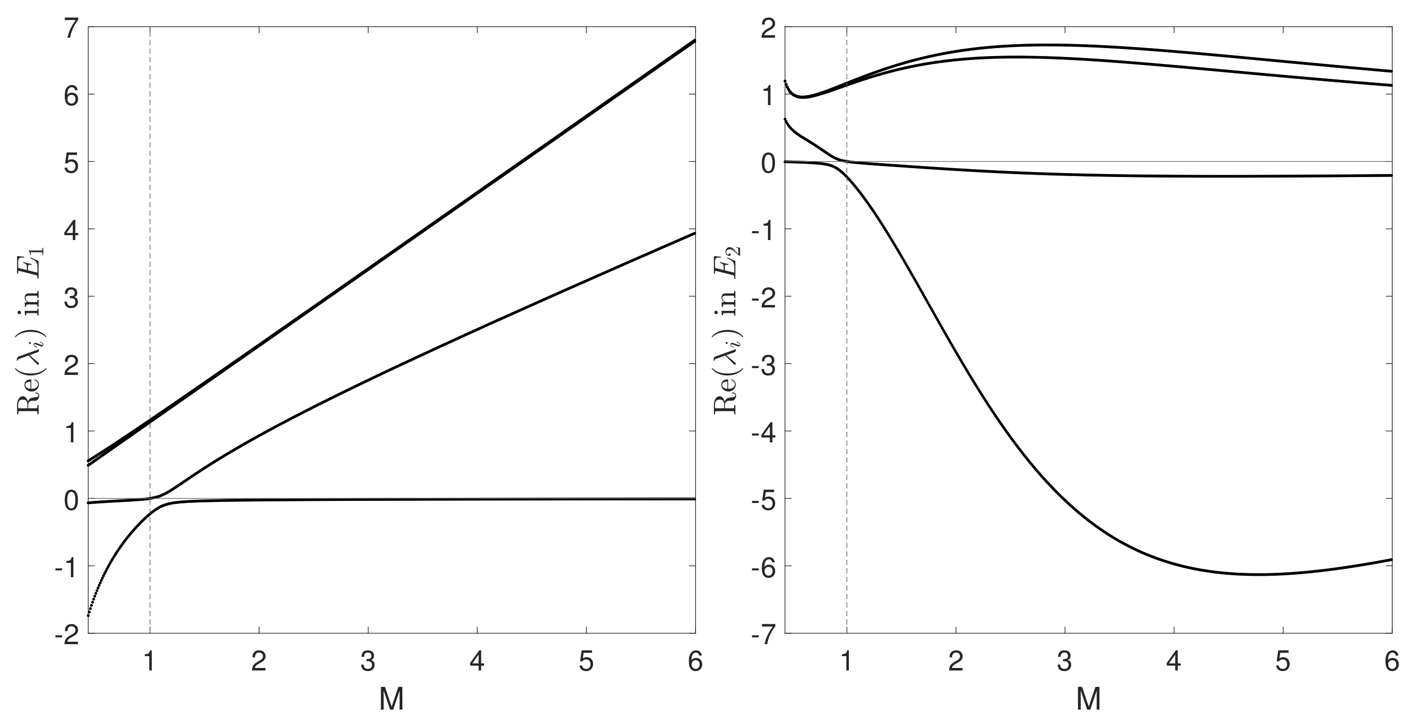
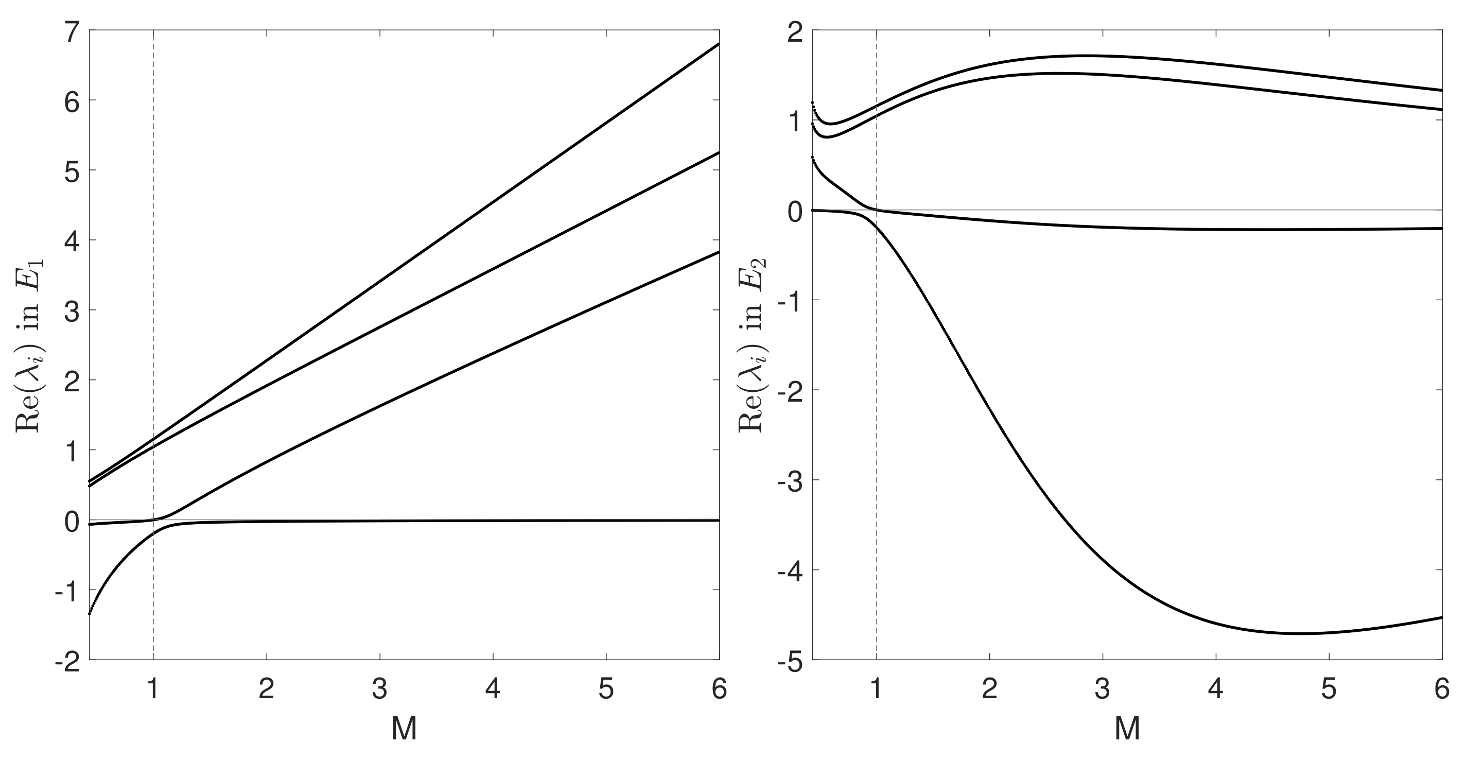
To carry on the investigation of stability of upstream and downstream steady states, the real part of eigenvalues of $J_{|E_1}$ and $J_{|E_2}$ versus Mach number will be computed owing to a proper Matlab routine, for varying parameters. In the reference case, the same values adopted in numerical simulations performed in the papers [30,31] are used: several degrees of freedom $\delta =4$, the Prandtl number $\mathrm{Pr}=0.761$ and the ratio of the bulk viscosity ${\mu }_b$ to the shear viscosity $\mu$ equal to 10, which correspond to $\nu =-0.33$ and $\theta =0.05$.

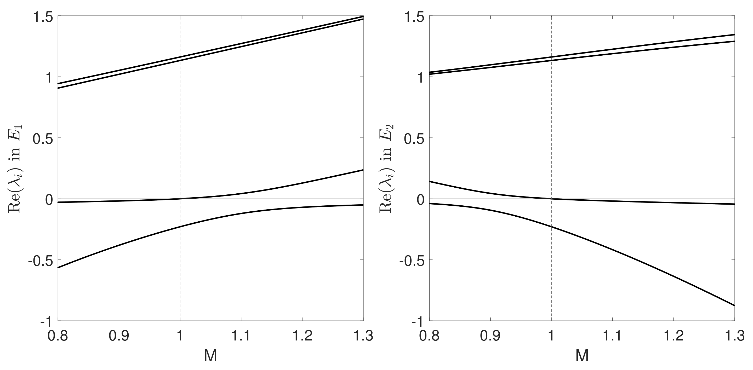
Figure 1 shows that in both equilibria one eigenvalue is close to 0. In the upstream equilibrium $E_1$ two eigenvalues of the Jacobian are very close to each other, but they are both real (a zoom of the results for $M\in [0.8,1.3]$ is plotted in Figure 2). For $\sqrt{\frac{\gamma -1}{2\gamma }}<M<1$, the upstream equilibrium $E_1$ has two positive and two negative real eigenvalues in its Jacobian (one of the negative ones is close to 0), while in the downstream equilibrium $E_2$ three eigenvalues are positive, and one is slightly below 0. Please note that $E_2$ is strongly unstable (the one-dimensional stable manifold corresponds to an almost vanishing eigenvalue), and this is consistent with the fact that in the subsonic regime the shock-wave solution connecting upstream and downstream equilibria is physically not admissible. On the other hand, for $M>1$, besides the almost vanishing (negative) eigenvalue due to the smallness of the parameter $\theta$, the equilibrium $E_1$ has three positive eigenvalues while $E_2$ has two positive and one negative eigenvalues. The shock-wave solution starting from $E_1$ should thus enter the stable manifold of $E_2$. Since $E_2$ is not asymptotically stable (the highest eigenvalue is positive), it is not easy to numerically capture the heteroclinic orbit which tends to $E_2$ for $x\to +\infty$. An analogous drawback occurs when reversing the x-axis (setting $\widehat{x}=-x$) and trying to construct the trajectory connecting $E_2$ to $E_1$; indeed, again $E_1$ is not an attractor, since the small eigenvalue becomes positive in the reverse setting. The plots corresponding to the same data of the reference case but with $\theta =0.0005$, choice adopted in the shock-wave figures reported in the paper [30], are not shown here, since results are very similar, but with an eigenvalue almost vanishing for any Mach (of the order of ${10}^{-3}$). Notice that in [30] the steady shock-wave profile has been obtained following a different approach, namely as the limiting (steady) solution of an evolution problem (with also time derivatives) having as boundary conditions the equilibrium states.

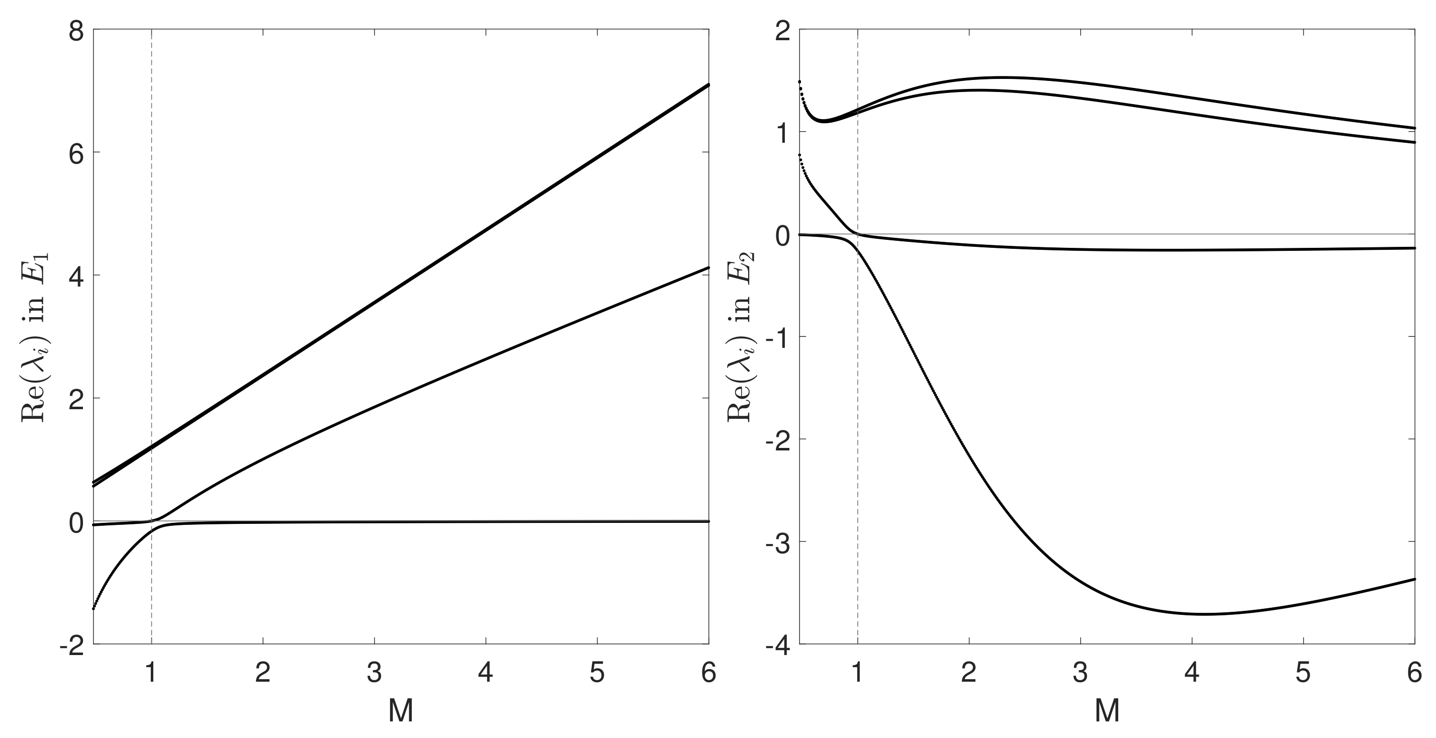
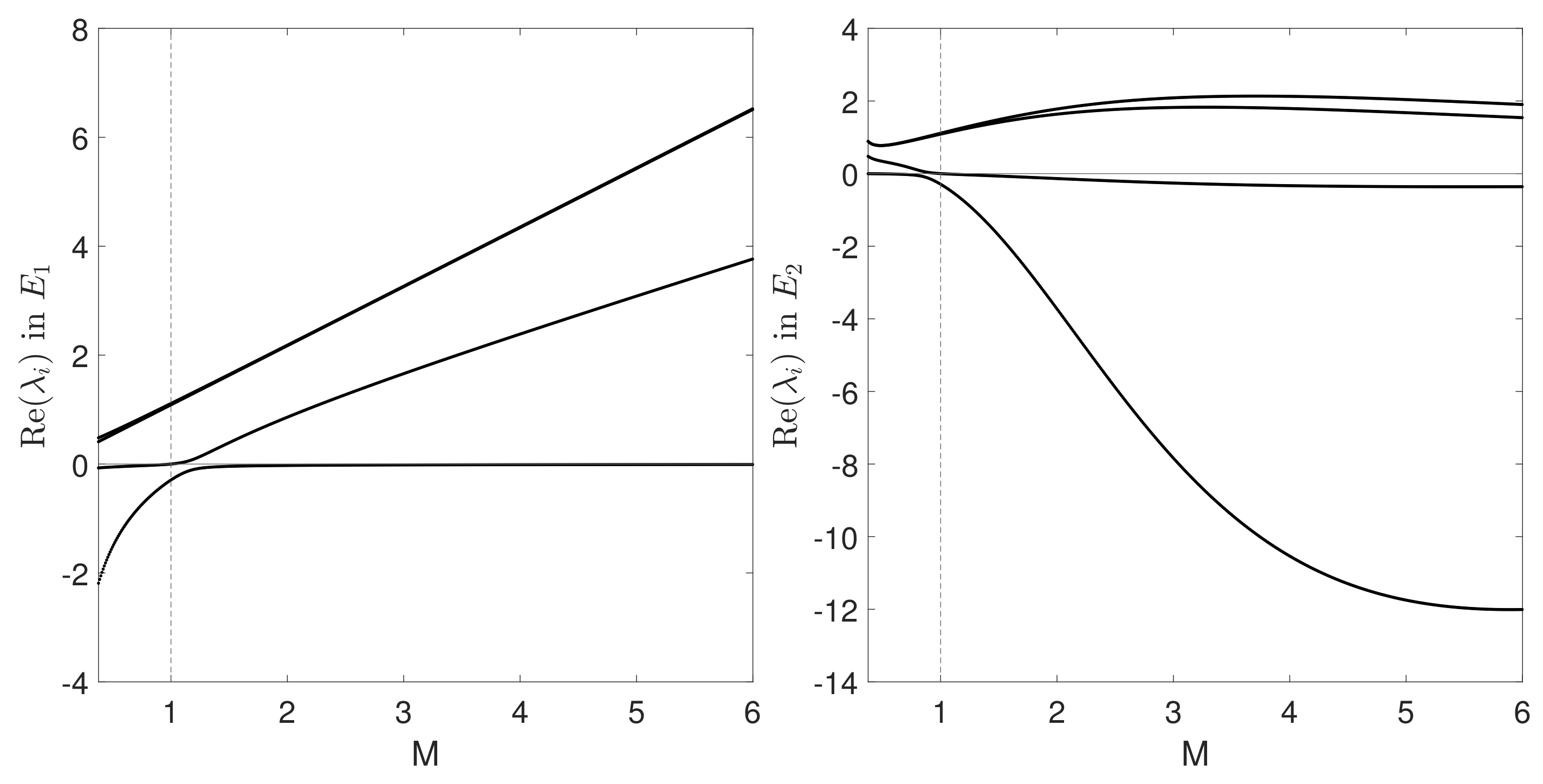
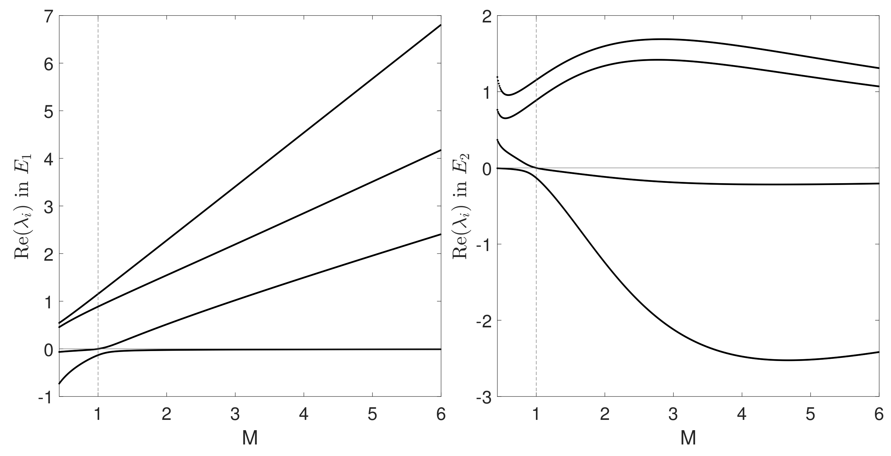
The number of degrees of freedom $\delta$ does not affect very much the nature of eigenvalues. See the case $\delta =2$ in Figure 3 and the case $\delta =8$ in Figure 4. The modulus of eigenvalues at equilibrium $E_1$ is slightly decreasing with respect to $\delta$, while the modulus of eigenvalues at $E_2$ increases versus $\delta$; however, the sign and the nature of each eigenvalue do not change.

Moreover, the trend of eigenvalues versus Mach number does not show evident changes even when the parameter $\theta$ becomes higher, namely in situations with bulk viscosity comparable to other transport coefficients. Figure 5 shows the case relevant to $\theta =0.3$ and $\mathrm{Pr}=0.761$, providing thus $\nu =-0.448$; note that in both equilibria the difference between the two highest eigenvalues is larger (hence more visible in the figures) than in the reference case. Of course, the physical validity of the present Navier–Stokes equations is not guaranteed in regimes with high $\theta$, since the Chapman–Enskog procedure leading from the kinetic to the hydrodynamic description was based on the assumption of $\theta$ with the same order of magnitude as the Knudsen number [30]. Moreover, high values of $\theta$ together with physical Prandtl numbers could provide $\nu$ lower than $-0.5$, not admissible for the ES–BGK model [14] described in Section 2; for instance, $\theta =0.5$ and $\mathrm{Pr}=0.761$ would yield $\nu =-0.628$.

Some changes in the modulus of eigenvalues and in the trends of the highest ones occur if the value for the parameter $\nu$ is increased with respect to the reference case. Figure 6 and Figure 7 show the results relevant to the options $\nu =0$ (corresponding to a classical isotropic BGK, see the tensor $\underline{\mathcal{T}}$ defined in (11)) and $\nu =0.5$, respectively.

It should be noted that all eigenvalues at upstream and downstream equilibria remain real for varying parameters, and the dimensions of stable and unstable manifolds remain the same as in the reference case. This latter result follows also from the determinant of the Jacobian matrix, given in (60), computed at the equilibria; indeed, a change in the sign of one eigenvalue would imply the change of sign also of the determinant, and this occurs only if $\theta$ becomes negative or $\nu$ exceeds 1 (not admissible options), or if one passes from the supersonic to the subsonic regime. The fact that both equilibria are unstable (even reversing the x-axis) implies that the construction of the shock-wave orbit as solution of the set of ODEs (49)–(52) is not easily manageable in practice from a numerical point of view; for this reason, the strategy presented in [30], which aims at obtaining the shock-wave solution as the limiting solution of a sort of Riemann problem, seems to be more suitable for the present frame.

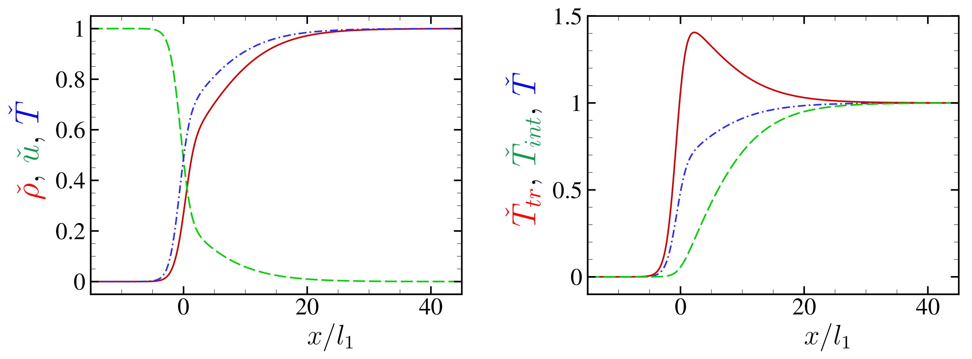
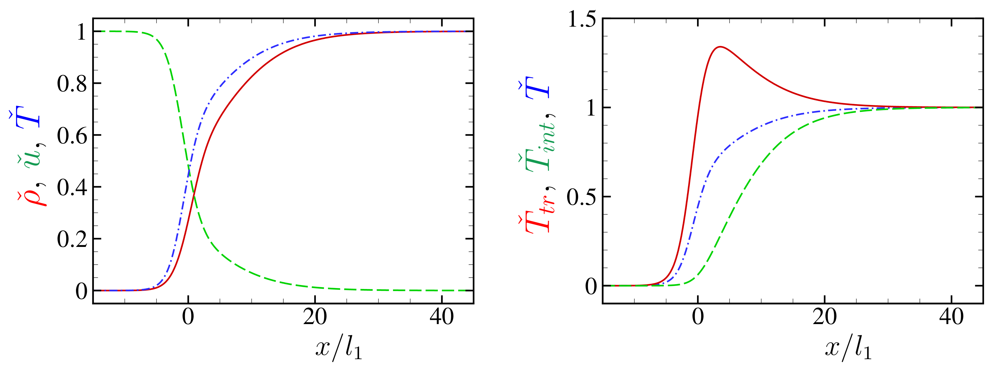
Using that procedure, the shock profiles for $M=2$ and parameters $\delta$, $\theta$, $\nu$ used in Figure 5, Figure 6 and Figure 7 are constructed; corresponding results are shown in Figure 8, Figure 9 and Figure 10, respectively. The numerical method is the same finite-difference scheme used in the paper [30], so details are skipped here. The domain is restricted to $-D_n\le \eta \le D_p$ and the grid points are chosen as ${\eta }_i$ ($i=-N_n,-N_n+1,\cdots ,0,\cdots ,N_p-1,N_p$) in such a way that ${\eta }_{-N_n}=-D_n$, ${\eta }_0=0$, and ${\eta }_{N_p}=D_p$; the length of the grid interval $[{\eta }_{i-1},{\eta }_i]$ is denoted by $\Delta {\eta }_i$, i.e., $\Delta {\eta }_i={\eta }_i-{\eta }_{i-1}$, and $t_n$ ($n=0,1,2,\cdots$) stands for the discrete time, i.e., $t_n=n\Delta t$ with $\Delta t$ being the constant time step. The values used in the present computations are $(D_n,N_n)=(56.4,1000)$, $(D_p,N_p)=(113,2000)$, $\Delta {\eta }_i=0.0564$, and $\Delta t=2.82\times {10}^{-4}$. In the figures, the plots of the normalized macroscopic fields

$$\check{\rho }=\frac{\rho -{\rho }_1}{{\rho }_2-{\rho }_1},\check{u}=\frac{u-u_2}{u_1-u_2},\check{T}=\frac{T-T_1}{T_2-T_1},{\check{T}}_{tr}=\frac{T_{tr}-T_1}{T_2-T_1},{\check{T}}_{int}=\frac{T_{int}-T_1}{T_2-T_1},$$

will be shown versus the normalized space variable $x/l_1$, where $l_1={(8R{T}_1/\pi )}^{1/2}/A_c\left(T_1\right){\rho }_1$ ( where $A_c\left(T\right)$ has been set to be constant). Denoting by $h_i^n$ the value of the function $h(t,\eta )$ at $t=t_n$ and $\eta ={\eta }_i$, where h indicates $\rho$, u, $T_{tr}$, etc., the following quantity is checked as a measure of accuracy of our computation

$$d=\underset{-N_n<i<N_p}{max}|({\rho }_i^n{u}_i^n-{\rho }_1{u}_1)/\left({\rho }_1{u}_1\right)|$$

(which should be zero theoretically); it turns out to be $d=1.2\times {10}^{-6}$ (in Figure 8), $1.3\times {10}^{-6}$ (in Figure 9), and $5.7\times {10}^{-6}$ (in Figure 10).

In Figure 8, corresponding to $\theta =0.3$, the profiles are smooth, and a temperature overshoot occurs for translational temperature $T_{tr}$. It is worth noting that in the present numerical simulation the convergence to the shock-wave solution is much faster than in cases discussed in the paper [30], corresponding to a smaller $\theta$ (of the order of ${10}^{-4}$ there): indeed, the parameter $\theta$, appearing on the right-hand side of equation for $T_{int}$, measures the relaxation speed of temperatures. On the other hand, in Figure 9 and Figure 10 where the value of the parameter $\nu$ is increased, a more evident difference appears between the values assumed by translational and internal temperatures in the intermediate part of the shock profile, and global temperature T, which may be seen as a weighted average of the two partial temperatures, shows a quite steep profile close to the upstream equilibrium, followed by a flatter tail reaching the downstream value.

For the values of M, $\delta$, and $\mathrm{Pr}$ in Figure 8, Figure 9 and Figure 10, the profiles should approach those with a double-layer structure composed of a thin front layer with a steep change and a thick rear layer with a slow relaxation, which is called Type-C profile in [32,47], as $\theta$ becomes small. This tendency can be observed in Figure 9 and Figure 10, where $\theta$ is relatively small ($\theta =0.05$).

5. Concluding Remarks

In this paper, the shock-wave structure has been investigated for a system of two-temperature Navier–Stokes equations, suitable for polyatomic gases with bulk viscosity much greater than shear viscosity, as CO${}_2$ [48]. Besides usual continuity equation and momentum equation, this set of PDEs contains two separate evolution equations for translational temperature $T_{tr}$ and internal temperature $T_{int}$. The steady version of the macroscopic system has been considered, and owing to conservation laws and to proper changes of variables, it has been transformed into a set of four independent first-order ODEs. Our analytical study of the shock-wave solution follows the ideas outlined in [45] which, in the frame of the evaporation–condensation problem, describes the shock-wave profile as the solution that remains bounded for all values of the space variable x, since it represents the heteroclinic orbit connecting the upstream equilibrium of the steady equations to the downstream one. The stability properties of such equilibria have been investigated, resorting to the qualitative theory of dynamical systems. In more detail, the signs of eigenvalues of the Jacobian matrix have been computed at upstream and downstream equilibria, by an analytical investigation of the matrix trace and determinant (sum and product of eigenvalues, respectively), and by means of numerical computations. It has been established that in the supersonic regime, with Mach number greater than one, the upstream state has a three-dimensional unstable manifold (which may give origin to the shock-wave profile), while the downstream one has a two-dimensional stable manifold (which may attract the heteroclinic orbit), therefore the existence of a shock-wave solution is possible. Moreover, it has been checked that an eigenvalue is of the same order of magnitude as the ratio between shear and bulk viscosities, therefore very small for CO${}_2$. Simulations for various values of the parameters involved in the kinetic model, such as the number of degrees of freedom $\delta$ and the parameters $\theta$ and $\nu$ contained in the original ES–BGK model, have been shown and commented on.

Since neither the upstream nor the downstream equilibria are asymptotically stable, it is quite difficult to numerically construct the shock-wave profile as a heteroclinic orbit for the set of ODEs. This difficulty in reaching the downstream state has already been pointed out in [49] for ordinary (one-temperature) Navier–Stokes equations. The situation is slightly better when the x-axis is reversed, since in this formulation the upstream equilibrium (to be reached for $-x\to +\infty$) has only one positive eigenvalue, with very small magnitude. However, the weak stability of equilibria suggests that the most suitable numerical strategy is the algorithm used in the paper [30], which recovers the shock wave as the steady solution of an evolution problem with proper boundary conditions (a sort of Riemann problem). The analysis performed in this paper allows thus to justify the use of a finite-difference scheme for an apparently much more complicated time-dependent problem to numerically provide a steady shock-wave solution. Such a numerical procedure has been adopted in this paper to show the shock-wave profiles even in cases with the ratio between shear and bulk viscosity much greater than in CO${}_2$. Therefore, the obtained profiles are not typical of the real CO${}_2$ gas. However, even if the ratio is not so small as in CO${}_2$ gas, the profiles tend to exhibit a double-layer structure, consisting of a thin front layer and a thick rear layer, which appears for CO${}_2$ gas [30,31,32,47] and is called Type-C profile in [32,47]. The presence of these profiles in other asymptotic regimes is worth investigating in the future, even starting from different kinetic models for polyatomic gases. Another interesting work, already in progress, concerns the derivation of suitable slip boundary conditions for the present macroscopic equations, following the procedure outlined in [24,50] for different Navier–Stokes systems. Moreover, this kind of analytical and numerical analysis could be repeated for other kinetic models. Indeed, a single ES–BGK model might not recover all possible situations. For instance, it has been shown that the models proposed in [14,20] cannot adjust the translational thermal conductivity, once the total thermal conductivity is fixed [51]; for this reason, they are not good enough to describe thermal transpiration, which is strongly related to translational (and not total) conductivity [52,53]. Different models are needed for this problem, in the spirit of the one proposed in [54] and possibly with also velocity-dependent relaxation frequencies, to take into account the influence of the intermolecular potential of the original Boltzmann collision kernel. The analysis of the shock-wave structure in these models would be also useful in view of applications.

References

- Cercignani, C. The Boltzmann Equation and Its Applications; Springer: New York, NY, USA, 1988. [Google Scholar]
- Giovangigli, V. Multicomponent Flow Modeling; Birkhäuser: Boston, MA, USA, 1999. [Google Scholar]
- Ruggeri, T.; Sugiyama, M. Rational Extended Thermodynamics beyond the Monatomic Gas; Springer International Publishing: Cham, Switzerland, 2015. [Google Scholar]
- Groppi, M.; Spiga, G. Kinetic approach to chemical reactions and inelastic transitions in a rarefied gas. J. Math. Chem. 1999, 26, 197–219. [Google Scholar] [CrossRef]
- Desvillettes, L.; Monaco, R.; Salvarani, F. A kinetic model allowing to obtain the energy law of polytropic gases in the presence of chemical reactions. Eur. J. Mech. B/Fluids 2005, 24, 219–236. [Google Scholar] [CrossRef]
- Arima, T.; Ruggeri, T.; Sugiyama, M. Extended thermodynamics of rarefied polyatomic gases: 15-field theory incorporating relaxation processes of molecular rotation and vibration. Entropy 2018, 20, 301. [Google Scholar] [CrossRef] [PubMed] [Green Version]
- Baranger, C.; Dauvois, Y.; Marois, G.; Mathé, J.; Mathiaud, J.; Mieussens, L. A BGK model for high temperature rarefied gas flows. Eur. J. Mech. B/Fluids 2020, 80, 1–12. [Google Scholar] [CrossRef] [Green Version]
- Bisi, M.; Cáceres, M.J. A BGK relaxation model for polyatomic gas mixtures. Commun. Math. Sci. 2016, 14, 297–325. [Google Scholar] [CrossRef]
- Bisi, M.; Monaco, R.; Soares, A.J. A BGK model for reactive mixtures of polyatomic gases with continuous internal energy. J. Phys. A Math. Theor. 2018, 51, 125501. [Google Scholar] [CrossRef] [Green Version]
- Bisi, M.; Travaglini, R. A BGK model for mixtures of monoatomic and polyatomic gases with discrete internal energy. Physica A 2020, 547, 124441. [Google Scholar] [CrossRef]
- Morse, T.F. Kinetic model for gases with internal degrees of freedom. Phys. Fluids 1964, 7, 159–169. [Google Scholar] [CrossRef]
- Rahimi, B.; Struchtrup, H. Macroscopic and kinetic modelling of rarefied polyatomic gases. J. Fluid Mech. 2016, 806, 437–505. [Google Scholar] [CrossRef] [Green Version]
- Struchtrup, H. The BGK model for an ideal gas with an internal degree of freedom. Transp. Theor. Stat. Phys. 1999, 28, 369–385. [Google Scholar] [CrossRef]
- Andries, P.; Le Tallec, P.; Perlat, J.P.; Perthame, B. The Gaussian-BGK model of Boltzmann equation with small Prandtl number. Eur. J. Mech. B/Fluids 2000, 19, 813–830. [Google Scholar] [CrossRef] [Green Version]
- Brull, S. An ellipsoidal statistical model for gas mixtures. Commun. Math. Sci. 2015, 13, 1–13. [Google Scholar] [CrossRef]
- Groppi, M.; Monica, S.; Spiga, G. A kinetic ellipsoidal BGK model for a binary gas mixture. EPL Europhys. Lett. 2011, 96, 64002. [Google Scholar] [CrossRef]
- Holway, L.H. Kinetic theory of shock structure using an ellipsoidal distribution function. In Rarefied Gas Dynamics; (Proc. Fourth Internat. Sympos., Univ. Toronto, 1964); Academic Press: New York, NY, USA, 1966; Volume I, pp. 193–215. [Google Scholar]
- Todorova, B.N.; Steijl, R. Derivation and numerical comparison of Shakhov and Ellipsoidal Statistical kinetic models for a monoatomic gas mixture. Europ. J. Mech. B/Fluids 2019, 76, 390–402. [Google Scholar] [CrossRef] [Green Version]
- Brull, S.; Schneider, J. On the ellipsoidal statistical model for polyatomic gases. Contin. Mech. Thermodyn. 2009, 20, 489–508. [Google Scholar] [CrossRef] [Green Version]
- Holway, L.H., Jr. New statistical models for kinetic theory: Methods of construction. Phys. Fluids 1966, 9, 1658–1673. [Google Scholar] [CrossRef]
- Mathiaud, J.; Mieussens, L. BGK and Fokker-Planck models of the Boltzmann equation for gases with discrete levels of vibrational energy. J. Stat. Phys. 2020, 178, 1076–1095. [Google Scholar] [CrossRef] [Green Version]
- Todorova, B.N.; White, C.; Steijl, R. Modeling of nitrogen and oxygen gas mixture with a novel diatomic kinetic model. AIP Adv. 2020, 10, 095218. [Google Scholar] [CrossRef]
- Chapman, S.; Cowling, T.G. The Mathematical Theory of Non-Uniform Gases, 3rd ed.; Cambridge University Press: Cambridge, UK, 1991. [Google Scholar]
- Hattori, M.; Kosuge, S.; Aoki, K. Slip boundary conditions for the compressible Navier–Stokes equations for a polyatomic gas. Phys. Rev. Fluids 2018, 3, 063401. [Google Scholar] [CrossRef]
- Bruno, D.; Giovangigli, V. Relaxation of internal temperature and volume viscosity. Phys. Fluids 2011, 23, 093104. [Google Scholar] [CrossRef] [Green Version]
- Kustova, E.; Mekhonoshina, M. Multi–temperature vibrational energy relaxation rates in CO2. Phys. Fluids 2020, 32, 096101. [Google Scholar] [CrossRef]
- Kustova, E.; Mekhonoshina, M.; Kosareva, A. Relaxation processes in carbon dioxide. Phys. Fluids 2019, 31, 046104. [Google Scholar] [CrossRef]
- Arima, T.; Ruggeri, T.; Sugiyama, M.; Taniguchi, S. On the six–field model of fluids based on extended thermodynamics. Meccanica 2014, 49, 2181–2187. [Google Scholar] [CrossRef]
- Bisi, M.; Ruggeri, T.; Spiga, G. Dynamical pressure in a polyatomic gas: Interplay between kinetic theory and extended thermodynamics. Kinet. Relat. Mod. 2018, 11, 71–95. [Google Scholar] [CrossRef] [Green Version]
- Aoki, K.; Bisi, M.; Groppi, M.; Kosuge, S. Two–temperature Navier–Stokes equations for a polyatomic gas derived from kinetic theory. Phys. Rev. E 2020, 102, 023104. [Google Scholar] [CrossRef]
- Kosuge, S.; Aoki, K. Shock-wave structure for a polyatomic gas with large bulk viscosity. Phys. Rev. Fluids 2018, 3, 023401. [Google Scholar] [CrossRef]
- Taniguchi, S.; Arima, T.; Ruggeri, T.; Sugiyama, M. Overshoot of the non–equilibrium temperature in the shock wave structure of a rarefied polyatomic gas subject to the dynamic pressure. Int. J. Non-Linear Mech. 2016, 79, 66–75. [Google Scholar] [CrossRef]
- Taniguchi, S.; Arima, T.; Ruggeri, T.; Sugiyama, M. Shock wave structure in rarefied polyatomic gases with large relaxation time for the dynamic pressure. J. Phys. Conf. Ser. 2018, 1035, 012009. [Google Scholar] [CrossRef]
- Pavic-Colic, M.; Madjarevic, D.; Simic, S. Polyatomic gases with dynamic pressure: Kinetic non–linear closure and the shock structure. Int. J. Non-Linear Mech. 2017, 92, 160–175. [Google Scholar] [CrossRef]
- Bisi, M.; Spiga, G. A two–temperature six–moment approach to the shock wave problem in a polyatomic gas. Ric. Mat. 2019, 68, 1–12. [Google Scholar] [CrossRef]
- Artale, V.; Conforto, F.; Martalò, G.; Ricciardello, A. Shock structure and multiple sub–shocks in Grad 10–moment binary mixtures of monoatomic gases. Ric. Mat. 2019, 68, 485–502. [Google Scholar] [CrossRef]
- Bisi, M.; Martalò, G.; Spiga, G. Shock wave structure of multi–temperature Euler equations from kinetic theory for a binary mixture. Acta Appl. Math. 2014, 132, 95–105. [Google Scholar] [CrossRef] [Green Version]
- Conforto, F.; Mentrelli, A.; Ruggeri, T. Shock structure and multiple sub-shocks in binary mixtures of Eulerian fluids. Ric. Mat. 2017, 66, 221–231. [Google Scholar] [CrossRef]
- Huang, S.; Wang, J.; Li, Z.; Wang, Y.; Jin, X.; Wang, K. Influence of an explosion air shock wave on arc quenching inside a cylinder. AIP Adv. 2020, 10, 025326. [Google Scholar] [CrossRef] [Green Version]
- Medici, E.F.; Allen, J.S.; Waite, G.P. Modeling shock waves generated by explosive volcanic eruptions. Geophys. Res. Lett. 2014, 41, 414–421. [Google Scholar] [CrossRef]
- Choi, J.Y.; Jeung, I.S.; Yoon, Y. Scaling effect of the combustion induced by shock–wave boundary-layer interaction in premixed gas. Symp. Combust. 1998, 27, 2181–2188. [Google Scholar] [CrossRef]
- Fedorov, A.F.; Shul’gin, A.V. Point model of combustion of aluminum nanoparticles in the reflected shock wave. Combust. Explos. Shock Waves 2011, 47, 289–293. [Google Scholar] [CrossRef]
- Kunova, O.V.; Nagnibeda, E.A. State–to–state description of reacting air flows behind shock waves. Chem. Phys. 2014, 441, 66–76. [Google Scholar] [CrossRef]
- Artem’eva, N.A.; Shuvalov, V.V. Interaction of shock waves during the passage of a disrupted meteoroid through the atmosphere. Shock Waves 1996, 5, 359–367. [Google Scholar] [CrossRef]
- Bobylev, A.V.; Ostmo, S.; Ytrehus, T. Qualitative analysis of the Navier-Stokes equations for evaporation–condensation problems. Phys. Fluids 1996, 8, 1764–1773. [Google Scholar] [CrossRef]
- Bisi, M.; Groppi, M.; Martalò, G. The evaporation–condensation problem for a binary mixture of rarefied gases. Contin. Mech. Thermodyn. 2020, 32, 1109–1126. [Google Scholar] [CrossRef]
- Taniguchi, S.; Arima, T.; Ruggeri, T.; Sugiyama, M. Thermodynamic theory of the shock wave structure in a rarefied polyatomic gas: Beyond the Bethe-Teller theory. Phys. Rev. E 2014, 89, 013025. [Google Scholar] [CrossRef] [PubMed]
- Cramer, M.S. Numerical estimates for the bulk viscosity of ideal gases. Phys. Fluids 2012, 24, 066102. [Google Scholar] [CrossRef] [Green Version]
- Elizarova, T.G.; Khokhlov, A.A.; Montero, S. Numerical simulation of shock wave structure in nitrogen. Phys. Fluids 2007, 19, 068102. [Google Scholar] [CrossRef] [Green Version]
- Aoki, K.; Baranger, C.; Hattori, M.; Kosuge, S.; Martalò, G.; Mathiaud, J.; Mieussens, L. Slip boundary conditions for the compressible Navier–Stokes equations. J. Stat. Phys. 2017, 169, 744–781. [Google Scholar] [CrossRef] [Green Version]
- Wang, P.; Su, W.; Wu, L. Thermal transpiration in molecular gas. Phys. Fluids 2020, 32, 082005. [Google Scholar] [CrossRef]
- Mason, E.A. Molecular relaxation times from thermal transpiration measurements. J. Chem. Phys. 1963, 39, 522–526. [Google Scholar] [CrossRef]
- Gupta, A.D.; Storvick, T.S. Analysis of the heat conductivity data for polar and nonpolar gases using thermal transpiration measurements. J. Chem. Phys. 1970, 52, 742–749. [Google Scholar] [CrossRef]
- Wu, L.; White, C.; Scanlon, T.J.; Reese, J.M.; Zhang, Y.H. A kinetic model of the Boltzmann equation for non–vibrating polyatomic gases. J. Fluid Mech. 2015, 763, 24–50. [Google Scholar] [CrossRef] [Green Version]
Figure 1.
Eigenvalues of the Jacobian (left) and (right) versus Mach number. Reference case, with , , which corresponds to .
Figure 2.
Zoom of the reference case described in Figure 1.
Figure 3.
Eigenvalues of the Jacobian (left) and (right) versus Mach number. Lower number of degrees of freedom: , , which corresponds to .
Figure 4.
Eigenvalues of the Jacobian (left) and (right) versus Mach number. Higher number of degrees of freedom: , , which corresponds to .
Figure 5.
Eigenvalues of the Jacobian (left) and (right) versus Mach number. Higher value of : , ; as in the reference case: it provides .
Figure 6.
Eigenvalues of the Jacobian (left) and (right) versus Mach number. Case with increased with respect to the reference case: , , (corresponding to ).
Figure 7.
Figure 8.
Profiles of , , , , and at in the case of , , and (, ). In the left figure, the solid line indicates , the dashed line , and the dash-dotted line ; in the right figure, the solid line indicates , the dashed line , and the dash-dotted line .
Figure 9.
Profiles of , , , , and at in the case of , , and (, ). See the caption of Figure 8.
Figure 10.
Publisher’s Note: MDPI stays neutral with regard to jurisdictional claims in published maps and institutional affiliations. |
© 2021 by the authors. Licensee MDPI, Basel, Switzerland. This article is an open access article distributed under the terms and conditions of the Creative Commons Attribution (CC BY) license (http://creativecommons.org/licenses/by/4.0/).
Share and Cite
MDPI and ACS Style
Aoki, K.; Bisi, M.; Groppi, M.; Kosuge, S. A Note on the Steady Navier–Stokes Equations Derived from an ES–BGK Model for a Polyatomic Gas. Fluids 2021, 6, 32. https://0-doi-org.brum.beds.ac.uk/10.3390/fluids6010032
AMA Style
Aoki K, Bisi M, Groppi M, Kosuge S. A Note on the Steady Navier–Stokes Equations Derived from an ES–BGK Model for a Polyatomic Gas. Fluids. 2021; 6(1):32. https://0-doi-org.brum.beds.ac.uk/10.3390/fluids6010032
Chicago/Turabian StyleAoki, Kazuo, Marzia Bisi, Maria Groppi, and Shingo Kosuge. 2021. "A Note on the Steady Navier–Stokes Equations Derived from an ES–BGK Model for a Polyatomic Gas" Fluids 6, no. 1: 32. https://0-doi-org.brum.beds.ac.uk/10.3390/fluids6010032