An Optimized-Parameter Spectral Clustering Approach to Coherent Structure Detection in Geophysical Flows


1
Department of Mechanical Engineering, Massachusetts Institute of Technology, Cambridge, MA 02139, USA
2
Physical Oceanography Department, Woods Hole Oceanographic Institution, Woods Hole, MA 02543, USA
*
Author to whom correspondence should be addressed.
Fluids 2021, 6(1), 39; https://0-doi-org.brum.beds.ac.uk/10.3390/fluids6010039
Submission received: 20 November 2020
/
Revised: 4 January 2021
/
Accepted: 8 January 2021
/
Published: 12 January 2021
(This article belongs to the Special Issue Lagrangian Transport in Geophysical Fluid Flows)
Abstract
:In Lagrangian dynamics, the detection of coherent clusters can help understand the organization of transport by identifying regions with coherent trajectory patterns. Many clustering algorithms, however, rely on user-input parameters, requiring a priori knowledge about the flow and making the outcome subjective. Building on the conventional spectral clustering method of Hadjighasem et al. (2016), a new optimized-parameter spectral clustering approach is developed that automatically identifies optimal parameters within pre-defined ranges. A noise-based metric for quantifying the coherence of the resulting coherent clusters is also introduced. The optimized-parameter spectral clustering is applied to two benchmark analytical flows, the Bickley Jet and the asymmetric Duffing oscillator, and to a realistic, numerically generated oceanic coastal flow. In the latter case, the identified model-based clusters are tested using observed trajectories of real drifters. In all examples, our approach succeeded in performing the partition of the domain into coherent clusters with minimal inter-cluster similarity and maximum intra-cluster similarity. For the coastal flow, the resulting coherent clusters are qualitatively similar over the same phase of the tide on different days and even different years, whereas coherent clusters for the opposite tidal phase are qualitatively different.
1. Introduction
In geophysical fluid flows, the Lagrangian approach, where one follows fluid parcels as they move through time and space, provides a natural perspective to study the dynamics of motion and the patterns of transport [1,2,3,4,5]. Even simple, time-periodic velocity fields can generate complicated trajectories and chaotic motion [6,7]. It thus comes as no surprise that Lagrangian transport in realistic oceanic flows, which are aperiodic, can be incredibly complex.
The Lagrangian structures that organize transport and govern coherent trajectory patterns are referred to as Lagrangian Coherent Structures (LCS), a term introduced by Haller and Yuan [8]. These structures act as the hidden skeleton of a flow [9,10] that can be uncovered using techniques from the dynamical systems theory [8,11,12]. Recent review papers of LCS detection methods include [13,14,15,16].
LCS methods can be classified into those looking to identify regions (two- and three-dimensional in 2D- and 3D-flows, respectively) with coherent Lagrangian motion, and those looking for the boundaries (one- and two-dimensional in 2D- and 3D-flows, respectively) between such regions. The majority of clustering methods, including our optimized-parameter spectral clustering presented in this paper, fall into the former category, whereas the latter category includes, for example, Finite-Time Lyapunov Exponent (FTLE) and Finite-Size Lyapunov Exponent (FSLE) ridges [8,17,18,19], geodesic and variational transport barriers [14,20,21,22], Lagrangian-Averaged Vorticity Deviation (LAVD) and Rotationally Coherent Lagrangian Vortices (RCLV) [23,24], and diffusive transport barriers [25].
Cluster-based LCS methods take root in the field of unsupervised machine learning. Several algorithms have been adapted recently to LCS detection in geophysical flows [26,27,28]. A recurring concern with these methods is that the results rely on a set of user-input parameters, making the outcome subjective. Hadjighasem et al. [15] present a comparison of the number of parameters required by several clustering methods to construct a Lagrangian field and show how spectral clustering requires the least amount of user inputs. The authors describe how to “choose a reasonable set of parameters for each method” to yield “the most favorable outcome”. They describe a robust outcome as an outcome where “small variations in the parameters do not lead to drastic changes in the outcome”, which is a fair way to describe robustness. The reasonability of the parameters and the favorability of the outcome, however, suggest that in the end, the user will have to make decisions about the outcomes of the analyses that could be arbitrary and subjective. In this paper, we append the conventional spectral clustering method of HA16 (explained in Section 2.1 and Section 2.2) with an algorithm for the automatic identification of the optimal parameters within pre-defined parameter ranges (Section 2.4). Our optimized-parameter spectral clustering method is still subject to all the usual limitations of the spectral approaches, including the need for a detectable spectral gap [15,29] and a tendency to favor clusters of equal size [30]. In addition to the parameter optimization algorithm for spectral clustering, we also introduce a noise-based metric for quantifying the coherence of the resulting coherent clusters (Section 2.4), which allows comparing the clusters to each other within the same flow, as well as inter-comparing the clusters between different flows. The optimized-parameter spectral clustering approach is then applied in Section 3 to two idealized analytical flows, the Bickley Jet and the asymmetric Duffing oscillator, and to a realistic oceanic coastal flow. In the last example, the identified clusters are tested using observed trajectories of real drifters. The results are discussed in Section 4.
2. Materials and Methods
Consider an unsteady flow that is known, either from measurements or simulations, over a finite-time window from to within a finite spatial domain. Our goal is to separate the domain into coherent clusters according to their Lagrangian behavior. Please note that the time window and the domain size should be considered part of the problem set up rather than parameters of the cluster detection method.
Below we review the conventional spectral clustering method, discuss its shortcomings associated with the need for user-input parameters, and then introduce a new and improved optimized-parameter spectral clustering method. We also review the Finite-Time-Lyapunov Exponents and Poincaré section techniques, which will be used in Section 3 for comparisons with the spectral clusters.
2.1. Conventional Spectral Clustering Method
The spectral clustering approach to LCS detection by [27], hereinafter referred to as HA16, partitions the dataset according to similarity between trajectories, such that intra-cluster similarity is maximized, and inter-cluster similarity is minimized. The similarity is determined from the pairwise distances between trajectories. Reviews of spectral clustering can be found in [29,31]. Below we briefly summarize the method.
Let and be two trajectories in , where for two- or three-dimensional flows, respectively, with positions at n discrete times from to . The time-averaged distance between trajectories is, following HA16:
with denoting the spatial Euclidean norm and where it is assumed that during each time step , the distance is constant and equal to the mean between the values at endpoints. Next, convert the pairwise distances into the similarity weights :
From the weights , build the similarity graph , with nodes , edges between nodes and , and similarity matrix that associates the weights to the edges . Next, define the sparsification radius r and sparsify W by removing all weights
The advantage of sparsifying W is two-fold: first, it saves computational efforts by removing a large number of entries; second, it minimizes the influences of entries with insignificant similarities.
The optimal partition of the domain is one with maximal intra-cluster similarity and minimal inter-cluster similarity; the ideal case would be one in which the dissimilarity between subsets is absolute, or the similarity is zero. The partition of the domain into k subsets that maximize the intra-cluster similarity and minimize the inter-cluster similarity can be achieved by minimizing the Ncut function, , where is a subset of the nodes within the domain, is the complement of and is the volume of set V, with . For large datasets, however, minimizing Ncut is computationally expensive. Therefore, an approximate solution is often used, which can be efficiently constructed with the eigenvectors of an eigenvalue problem for the graph Laplacian (see [29,31] for derivations of this result):
where the diagonal degree matrix, D, contains degrees, , for all nodes . The solutions s are the generalized eigenvectors associated with the unnormalized graph Laplacian L from Equation (4). As detailed in [29], it is often advantageous to use a normalized Laplacian: normalized spectral clustering performs better in partitioning the graph such that within-cluster similarity is maximized, especially for irregular graphs with vertices of highly varying degrees. We thus use the normalized graph Laplacian
following the derivation in HA16. Hereinafter, the ’s refer to the eigenvectors of the normalized graph Laplacian .
From perturbation theory and the Davis–Kahan theorem, which bounds the differences between eigenspaces of symmetric matrices under perturbations, the eigenvectors ’s are close to the vectors from the exact Ncut partition. The order of eigenvectors and eigenvalues is meaningful and the first k eigenvectors s can be used as approximate solutions for the k connected components of the graph. The optimal number of eigenvectors that are kept is retrieved by the heuristic argument of the spectral eigengap, i.e., the largest gap between successive eigenvalues of . This number equals the number of eigenvalues before the eigengap. The resulting partition separates the connected components from the rest of the domain, which is assigned to the ”incoherent background” subset. The wider the eigengap, the closer the approximate solution is to the exact solution of the graph cut minimization problem and the better the partition of the domain will be.
The final step is to extract the coherent clusters from the weighted graph data. To partition N trajectories, or nodes, into clusters (i.e., into coherent clusters and 1 incoherent background cluster), the K-Means algorithm ([32], summarized below) is applied to the matrix of the first eigenvectors . Each eigenvector has length N (for the N nodes), and the matrix U has size N-by-. U contains information about the connectivity between nodes within the connected part of the graph. The output of K-Means is an N-by-1 vector that assigns a cluster index of each node. The clusters are mutually exclusive, i.e., each node only belongs to 1 cluster. For this reason, the K-Means is sometimes referred to as Hard C-Means, in contrast to the Fuzzy C-Means clustering, where a node can be assigned to different clusters with some probability.
The K-means iterative algorithm is applied to U as follows:
1. randomly assign each node to a cluster;
2. compute the cluster centers for all clusters:
where the first summation goes over all nodes n belonging to cluster k and where is the number of nodes in cluster k;
3. compute the sum of inter-cluster distances from the corresponding cluster centers:
4. compute distances from each node to all cluster centers
and assign each node to the cluster with the closest center;
5. repeat steps 2–4 until the cluster assignment does not change or until the improvement in is below a tolerance threshold. Then, output the cluster assignment.
In the spectral clustering approach, the K-Means algorithm is not applied to the flow trajectories, but to the eigenvectors of the graph Laplacian . The clustering of spectral vectors as opposed to a trajectory dataset is the key difference with other clustering methods for LCS detection, including the Fuzzy C-Means approach by [26].
2.2. Challenges of Conventional Spectral Clustering
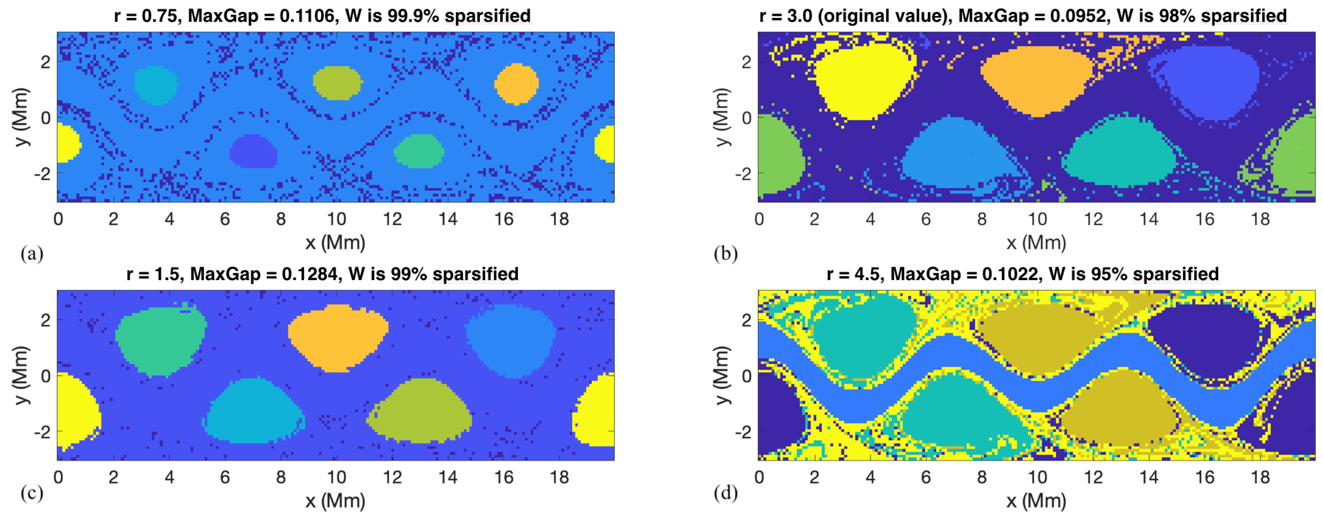
One important shortcoming of the conventional spectral clustering is the need for user-input parameters, including the sparsification radius r in Equation (1) and the percentage of sparsification in W, both of which significantly affect the spectral clustering results. For r, HA16 advise to choose the r value which, first, sparsifies the weights matrix by 5–10% (so that 90–95% entries are removed during the sparsification step), and second, the optimal r should correspond to the largest eigengap. As illustrated in Figure 1, however, the largest eigengap is often achieved at an r value that contradicts the 5–10% sparsification rule of thumb, and in many problems corresponds to the largest r considered. Thus, in the end, the choice of r is left entirely to the subjective judgement of the user and relies on the a priori knowledge of the system under study.
Another user input is the distance function and, subsequently, how it impacts the diagonal elements in W. [31] use a Gaussian kernel for the distance between nodes, a commonly chosen function in spectral clustering [30], and choose an offset value for the diagonal of elements in W. HA16 use a different approach, where the distance function is described by Equation (2) and the offset is added to W before computing D. This offset value in the diagonal elements is set to a large constant, which is immaterial for unnormalized graph Laplacians. Normalized Laplacians are however more common and adding the offset for the adjacency matrix W before calculating D does affect the eigenvalues and eigenvectors. The reader should thus be mindful of the scalar chosen for this diagonal offset, as it can impact the spectral clustering results.
Very large values (towards ) of the offset can introduce numerical errors due to the limits of double-precision. On the opposite, an offset value that is too small compared to the other ’s entries of W can yield erroneous results. Unlike r, the offset is not a real physical parameter, but rather a numerical manipulation to avoid infinity in the diagonal. A convergence in the spectral decomposition is expected for large values of the offset, as long as these scalar values are numerically reasonable. ‘Large’ values, however, will depend on the flow: for this reason, the proposed approach verifies the convergence of the results and sets the offset value as a coefficient related to the maximum entry in W, as described in more detail below.
2.3. Improved Optimized-Parameter Spectral Clustering
Here we propose an improvement to the conventional spectral clustering algorithm, which minimizes the need for user-input parameters. The optimal parameter choices are based on the notion of convergence (for ) and an argument involving the normalized spectral eigengap (for r). With and r obtained in a user-independent fashion within pre-defined ranges, the sparsification number is no longer needed. With these modifications, the only user input is the pre-defined range for parameters, within which the method automatically detects optimal parameter values. We also provide guidance for the choice of the parameter range that is most inclusive and worked well in all our examples.
The sparsification radius r defines the largest allowed distance between trajectories, because all weights corresponding to larger distances are removed during sparsification. Thus, r can be thought of as the parameter defining the size of the resulting clusters. It is tempting to use the same eigengap argument to define the optimal r, which was used to define the optimal number of clusters , namely that the optimal r should yield the largest eigengap. The eigenvalues of the graph Laplacian, and thus the corresponding eigengap value, however, typically decrease with r, as more and more entries are removed from the weight matrix during sparsification. Thus, the r value that yields the largest eigengap is often the largest r considered. To overcome this issue and use the spectral gap arguments for choosing the optimal r, we introduce the normalized spectral eigengap by referencing the largest eigengap to the full dynamic range of the spectral values. Specifically, we define the normalized eigengap as the absolute value of the maximum eigengap divided by the difference between the largest and smallest eigenvalues, :
This is similar in spirit to the recently proposed Normalized Maximum Eigengap by [33], but in our approach the denominator is automatically calculated from the spectral decomposition and does not include any user-input coefficient. As normalization does not change the physical meaning of the eigengap, large values of the normalized eigengap still yield spectral clusters with high intra-cluster similarity and low inter-cluster similarity. The optimal r should result in clusters with higher/lower intra-/inter-cluster similarity than those for both locally smaller or larger r values. Thus, the optimal r values should correspond to local maxima in the normalized eigengap. If several local maxima are present, we suggest proceeding with identifying coherent clusters for all the corresponding r values. This will ensure that in flows with more than one dominant length scale, all coherent clusters of different sizes will be recovered. Since a reliable estimate of a coherent cluster requires at least several trajectories within it, the smallest r considered should be dictated by the resolution, i.e., by the number of trajectories released in the domain and the distance between neighboring trajectories. In all our simulations, the simulated trajectories are released on a regular rectangular grid spanning the domain and the trajectory grid spacing is the initial distance between neighboring simulated trajectories. As a rule of thumb, we propose starting the r search with a value 10 times larger than the trajectory grid spacing. At smaller values of r, the number of nodes within the r radius is very low, which can result in computations on subsets with new nodes only; such small clusters may be erroneous and numerically unstable. Finally, r values approaching the domain size will result in the nearly entire domain being assigned to one cluster, and while this partition has high intra- and low inter-cluster similarity, it is trivial and not physically relevant. Choosing r values that correspond to the local maxima in normalized eigengap (and not the largest value of the normalized eigengap) avoids this problem. Although the normalized eigengaps can be also high for both very small and very large values of r, they are not peaks; peaks, rather, indicate that structures at the corresponding r value are more connected in comparison to the incoherent background than the structures at neighboring values of r. Thus, these are the structures that are of most interest to us.
We now describe the strategy for eliminating the need for choosing the user-input parameter . In practice, the offset value chosen for the diagonal of W impacts the spectral clustering results. Being the artificial parameter introduced for numerical stability considerations, convergence of results is expected for increasing values of w (HA16). However, while w should be substantially higher than the rest of the weights, excessively large ws result in numerical errors due to the limits of double-precision. Insufficiently large values of the offset will also yield erroneous results. Finally, the offset depends on the flow under study, and what is large for one system may be small for the other. For this reason, we propose to seek the optimal flow-dependent offset value of the form:
with integer n, and pick n which corresponds to the smallest value at which convergence of the results, specifically, convergence of the normalized spectral eigengap, is achieved.
With w and r determined based on the normalized eigengap arguments as outlined above, and the number of clusters K defined by the number of eigenvalues before the eigengap (), the new spectral clustering protocol does not require any other user input to find the optimal partition of the domain. Note, however, that the user still needs to pre-define the range over which the algorithm will look for the optimal parameters, as well as to choose the parameter increment for the parameter sweeps, so our optimized-parameter method cannot be considered entirely parameter-free.
As with all spectral methods, the proposed optimized-parameter spectral clustering requires the existence of a detectable spectral gap. As detailed in [29], the larger the eigengap, the better the spectral clustering partition will be in terms of yielding large/small intra-/inter-cluster similarity. Note, however, that we do not impose an explicit threshold on how large the spectral gap should be. Instead, we simply define the normalized spectral gap as the largest gap between successive eigenvalues of the normalized eigenspectrum. Thus, our optimized-parameter spectral clustering method can be applied to any flow (except the degenerate case when the eigenspectrum is completely flat) and will identify a partition of the domain into coherent clusters based on the eigengap heuristic, but the values of the normalized eigengap should be taken into consideration when interpreting the resulting clusters and the associated partition of the domain. Note also that in addition to the values of the normalized eigengap, the proposed noise-based coherence metric (introduced below in Section 2.4) can also be used to quantify the robustness of the detected features and their sensitivity to numerical noise and observational or model uncertainty.
2.4. Noise-Based Cluster Coherence Metric
Once the spectral clustering analysis is conducted, how coherent are the resulting clusters? The eigenvalues of the graph Laplacian contain information about coherence of eigenvectors but not of spectral clusters, because there is no one-to-one correspondence between former and latter. The spectral eigengap value, on the other hand, contains information about how optimal the partition is in terms of minimizing/maximizing inter-/intra-cluster similarity, but it does not provide information about the coherence of individual clusters. In many applications, such as identifying an optimal field experiment design or a strategy for a search-and-rescue operation, it is the coherence of individual clusters that determines the drifter release strategy or the search pattern. To determine how coherent the clusters are, we define below one possible coherence metric that is based on the robustness of the clusters with respect to a small random perturbation. This applied numerical noise can be representative, for example, of uncertainties in ocean circulation models. Our metric is similar, in spirit, to the approach by [34]. The robustness to noise is computed as follows. For trajectories starting at inside a given cluster, randomly perturb their final positions at time , and advect trajectories backward in time to the start time . The percentage of trajectories that return within the boundaries of their cluster is the proposed coherence metric. In all numerical simulations, we use the noise magnitude equal to th of the trajectory grid spacing (here, the grid spacing is the initial distance between neighboring trajectories, as defined in Section 2.3) but the results are similar for slightly larger or smaller perturbations. Essentially, our noise-based coherence metric favors coherent sets with large area-to-perimeter ratio and thus punishes small and filamentated clusters. Please note that because our coherence metric is not used to detect coherent clusters, it is not a parameter of our spectral clustering method. Rather, the coherence metric is computed after the clusters have been identified, and it allows us to interpret and inter-compare the robustness of the detected clusters with respect to noise.
2.5. Optimized-Parameter Spectral Clustering Algorithm Summary
The application of the optimized-parameter spectral clustering consists of 3 steps:
- r-sweep: compute the normalized eigengap for variable sparsification radii r, from × (trajectory grid spacing) to (the domain size), keeping the fixed offset value (× worked well in all examples), and identify all local maxima. This choice of the upper limit, , is the most inclusive as it allows detecting clusters that are as large as the entire domain. This choice of the lower limit, , ensures that clusters contain at least 10 nodes (to avoid detecting of very small clusters that might be numerically unstable.)
- w-sweep: for all local maxima, verify the convergence in the normalized eigengap by varying × , . In all our examples, convergence was observed at , but we cannot guarantee that this is true for all flows. If the normalized eigengap still varies between and , increase n past the value of 10 to ensure convergence.
- identify coherent sets corresponding to all local eigengap maxima and compute noise-based coherence metrics for the resulting clusters.
2.6. Finite-Time Lyapunov Exponents and Poincaré Sections
In the next section, we also use Finite-Time Lyapunov Exponents (FTLE) and Poincaré sections to provide insight about the flow and to compare with the coherent clusters obtained using the optimized-parameter spectral clustering. For completeness, below we briefly describe both methods.
Poincaré section is a technique that allows mapping the chaotic and non-chaotic (regular) regions of the domain in time-periodic flows by stroboscopically sampling trajectories after each period of the perturbation. On the Poincaré section, regular trajectories appear as discretely sampled smooth curves, and chaotic trajectories appear as clouds of dots covering finite areas.
The FTLE approach [8,14,17] is probably the most widely used LCS detection method due to its intuitive nature and numerical robustness. FTLE fields can be computed by the differentiation of the flow map, , obtained from numerical trajectories that start at and advected by the flow over a finite integration time . Specifically, the gradient of the flow map is used to compute the Cauchy-Green strain tensor, , whose largest eigenvalue, , quantifies the largest amount of stretching between neighboring trajectories and is then used to construct the FTLE field Maximizing ridges of the FTLE field reveal the locally most repelling LCSs (provided that particle separation is dominated by strain and not shear; see Haller [14]), which are the finite-time counterparts of the invariant stable manifolds of hyperbolic trajectories in time-periodic flows. Similarly, maximizing ridges of the backward FTLEs reveal the most attracting LCSs.
3. Results
In this section, the new optimized-parameter spectral clustering method is applied to three flows with increasing complexity: the analytically prescribed Bickley Jet (with coherent sets of the same size), the analytically prescribed asymmetric Duffing oscillator (with coherent sets of different sizes), and a numerically generated realistic coastal flow from the ocean circulation model MSEAS. In the latter case, spectral clusters from a model are compared against trajectories of real drifters.
3.1. Bickley Jet
The Bickley Jet flow consists of a zonal jet on which 2 traveling Rossby waves are superimposed. Following [35], we use the streamfunction
where ms is the velocity at the jet core; km is the characteristic jet width scale; are wavenumbers with the Earth radius, and are wave phase speeds; and and are wave amplitudes. In the reference frame moving with , the flow consists of a steady background and a time-periodic perturbation:
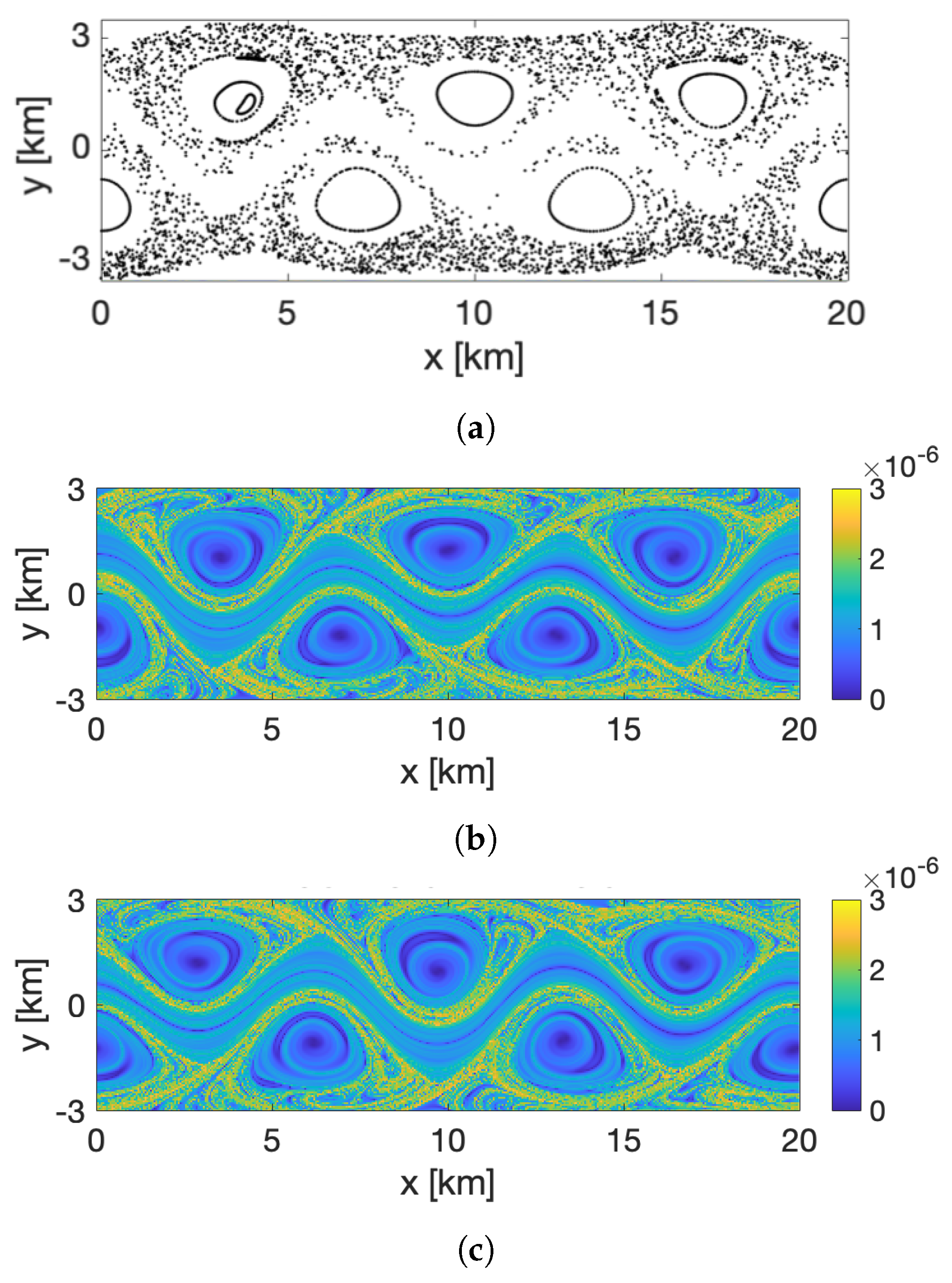
with. The Poincaré map (computed over 1000 perturbation periods) and the forward-/backward- FTLEs (computed over 30 perturbation periods) for this flow are shown in Figure 2a. The regular (i.e., non-chaotic) meandering jet separates two chaotic zones to the north and south, with 3 regular vortices embedded into each chaotic zone. Between the vortices there exist 3 hyperbolic trajectories with stable and unstable manifolds that form heteroclinic tangles. HA16 also used the Bickley Jet as a benchmark flow but with an extra (3rd) wave with and in (13). We chose the 2-wave Bickley Jet for the benefit of comparing spectral clusters with the Poincaré section.
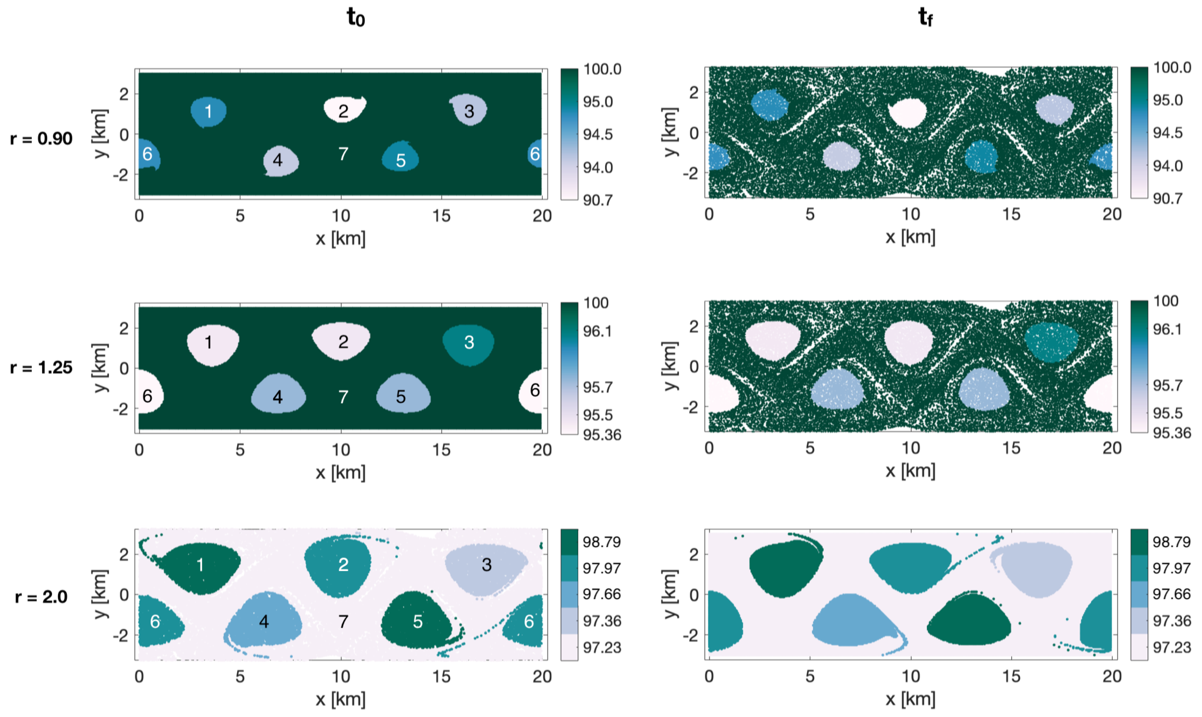
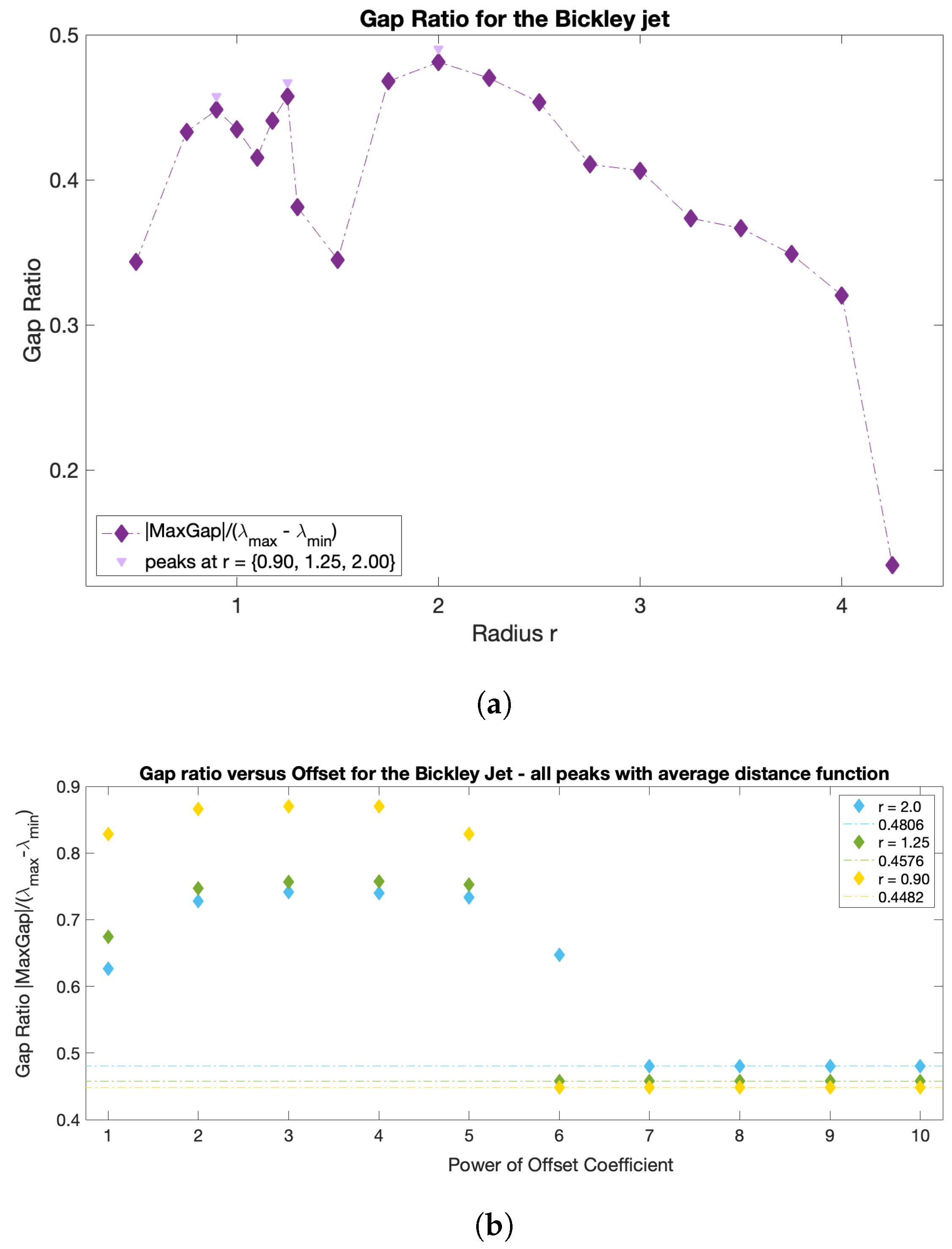
Following the proposed optimized-parameter spectral clustering approach, we performed sweeps in the sparsification radius r (from 0.5 to 4.25 with an incremental step of 0.25, and with finer steps around the detected peaks) and sweeps in the offset coefficient w ( with integer n from 1 to 10). The resulting normalized eigengap shows 3 local maxima in r (0.90, 1.25 and 2.0), yielding clusters in all 3 cases. For all r, the normalized eigengap converges at . (See Figure A1a,b in Appendix A.1) The coherent clusters, color-coded by their noise-based coherence metric, for all 3 peaks in r are shown in Figure 3. In all cases, the method successfully detected 6 vortices centered at each of the 6 regular islands in the Poincaré map. The sizes of the detected clusters grow with r, which is fully consistent with our interpretation of r as the parameter responsible for the cluster size. For and , vortices are smaller and less filamented than for . In the latter case, each vortex contains one long and narrow filament. Note, however, that when advected to the final time , identified coherent vortices do not get filamented any stronger than at , whereas for an arbitrary subset, the degree of filamentation generally increases with time. The noise-based coherence metric suggests high coherence (>90%) for all the detected coherent clusters, as well as for the incoherent background. The coherence is lower for smallest clusters (corresponding to ) due to their smaller area-to-perimeter ratios. For and , the coherence metric for the incoherent background exceeds that of the 6 vortices and nearly reaches 100%, but at it drops to a value that is below that for the vortices. This is likely due to a combination of the filamentation and smaller area-to-perimeter ratio for the incoherent background at . Advecting the clusters beyond the final time of the integration window shows that the cluster with the lowest coherence metrics (cluster 3, 97.36%) starts deteriorating before the other clusters, as early as 40.5 days, whereas cluster 5, with the highest coherence metrics of 98.79%, starts deteriorating around 46.5 days.
3.2. Asymmetric Duffing Oscillator
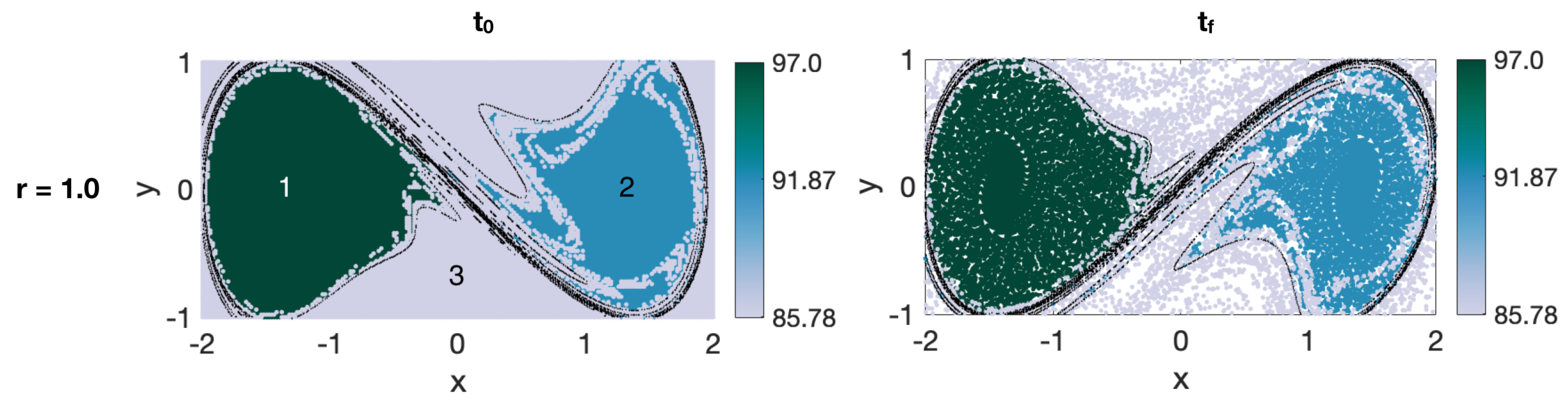
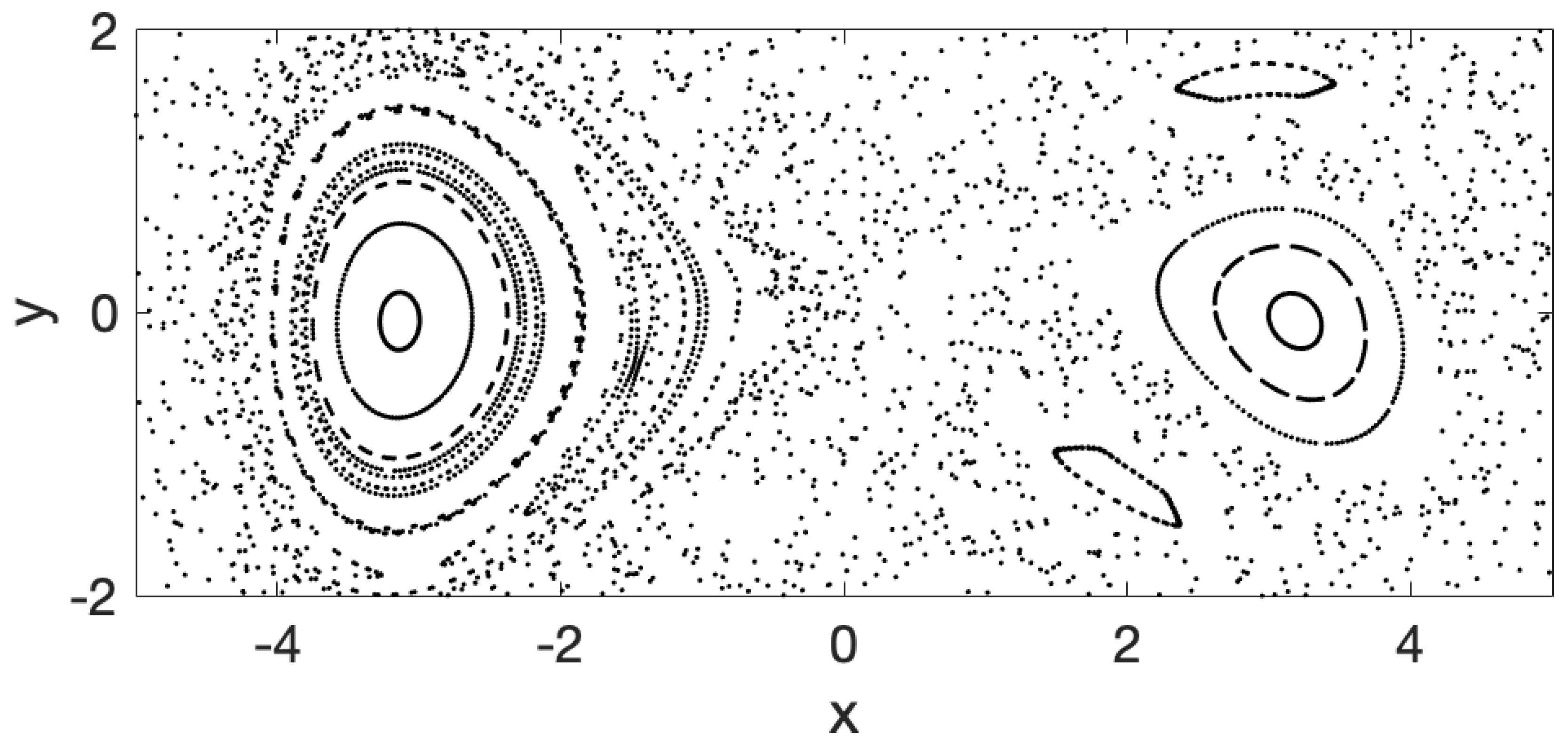
To test the method on a system with coherent sets of different sizes, we use an asymmetric Duffing oscillator. The Duffing oscillator is another commonly used benchmark flow that consists of two gyres with the same sign of rotation located on opposite sides of the hyperbolic point at the origin [36]. The classic Duffing oscillator has two identical gyres of same size. Here, we use a longitudinal asymmetry to generate a right gyre that is smaller than the left gyre. When the gyres oscillate around their mean position periodically with time, the stable and unstable manifolds of the hyperbolic trajectory form a homoclinic tangle that induces chaos in a figure-eight-shaped chaotic region around the gyres. The asymmetric Duffing oscillator velocity is two-dimensional, incompressible and is described by a streamfunction
with
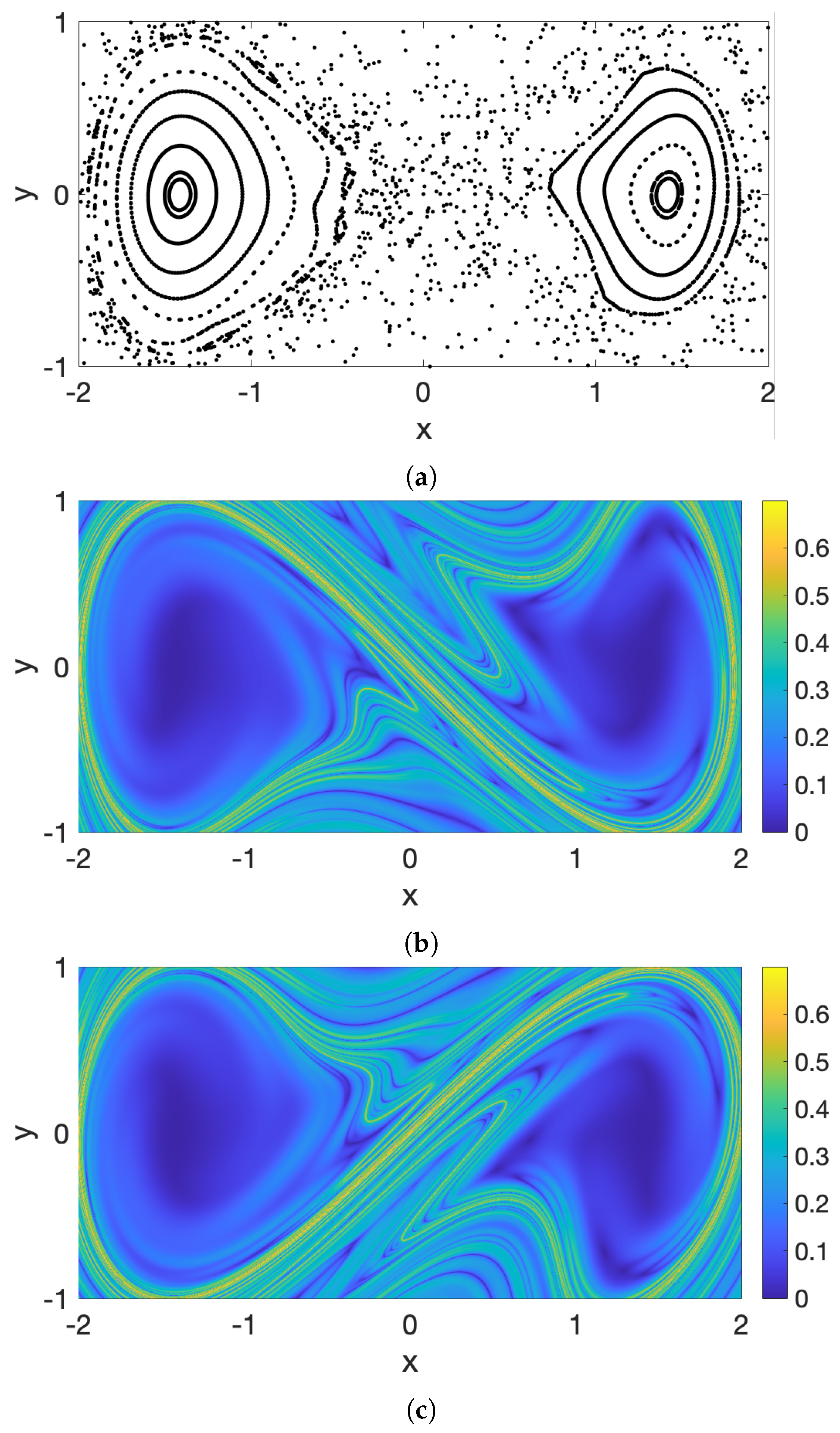
Here, , , and . The corresponding Poincaré map and FTLE fields are shown in Figure 4.
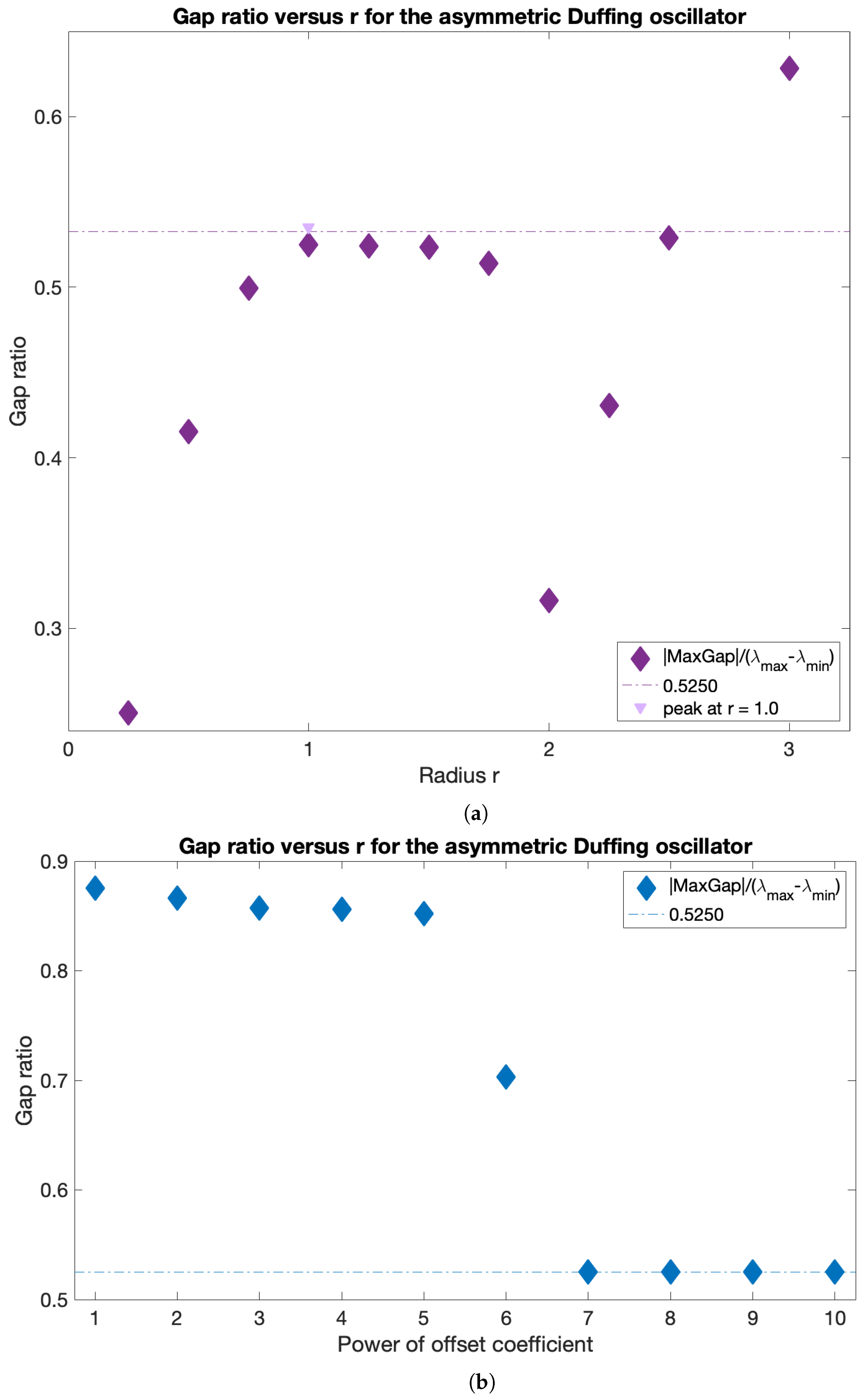
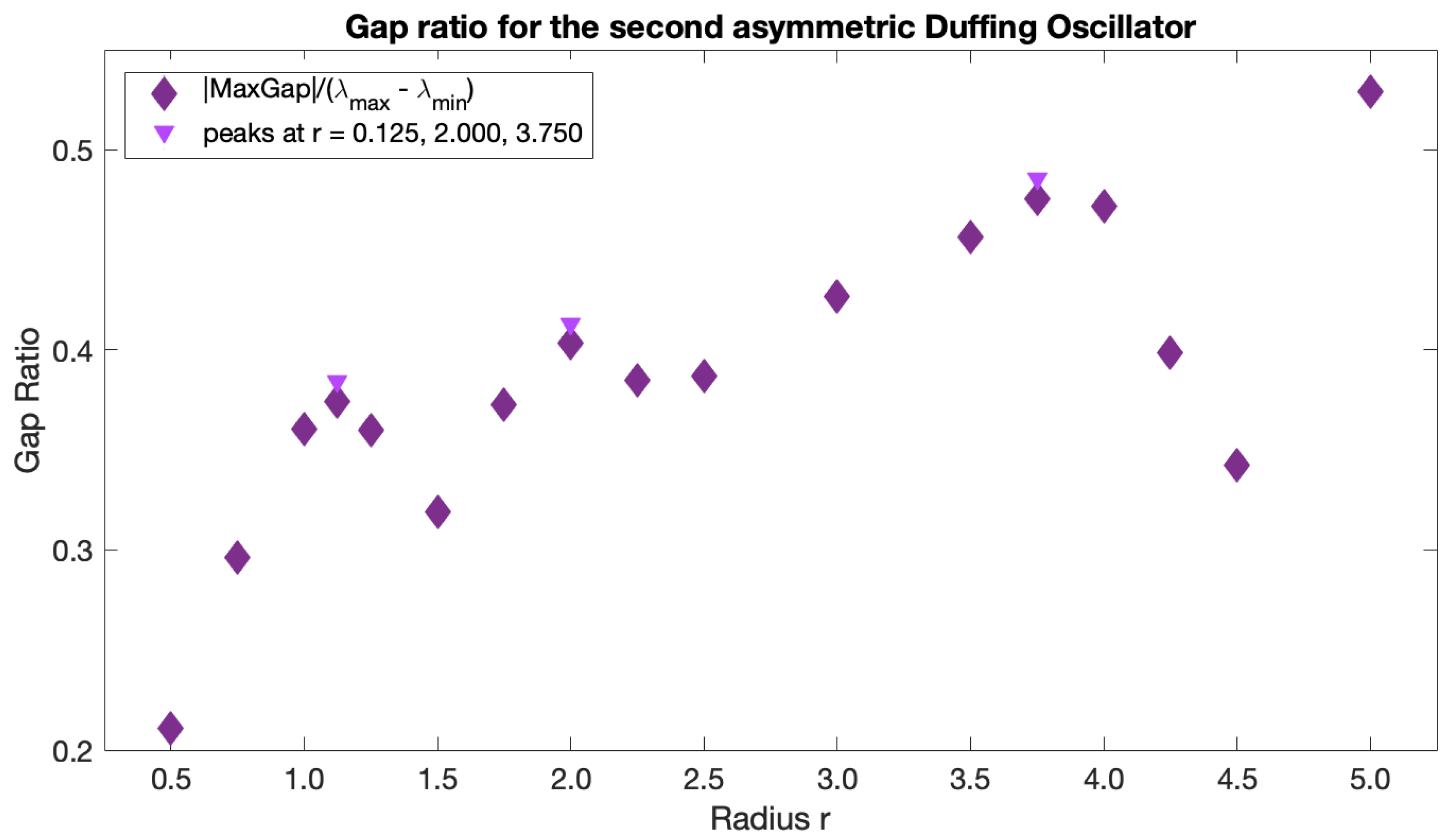
To identify coherent sets we again followed the optimized-parameter spectral clustering algorithm described in Section 2. The analysis revealed one peak in the normalized eigengap at (Figure A2a in Appendix A.2) with eigenvalues before the eigengap. Convergence of the normalized eigengap with respect to the increasing values of the offset parameter is achieved at (Figure A2b in Appendix A.2), the same value of as for the Bickley Jet.
The resulting two clusters plus the incoherent background, color-coded by their noise-based coherence metrics, are shown in Figure 5. As expected, the clusters correspond to the two gyres, the larger gyre on the left and smaller on the right. Both coherent clusters, but especially the right cluster, in this example are more filamented than for the Bickley Jet flow. Nevertheless, the cluster coherence is still high, about 92 and 97%, which is above that of the incoherent background (about 86%). Interestingly, at initial time ,the filaments are approximately aligned with the stable manifolds (black curve in Figure 5, left), outlining the turnstile lobes in such a manner that when advected forward to , filamentation of the clusters does not increase. Overall, in this example the optimized-parameter spectral clustering performed well at identifying coherent clusters of slightly different sizes and partitioning the domain into subsets with high intra- and low inter-cluster similarity. The application of the optimized-parameter spectral clustering to the flow where cluster sizes are very different is shown in Appendix B.
3.3. Geophysical Example: Flow Around No Man’s Land Island
In 2017 and 2018, two field experiments took place in coastal waters south of Martha’s Vineyard, MA as part of the NSF-funded Advanced Lagrangian Predictions for Hazards Assessments (ALPHA) project. The goal of the project was to develop and test Lagrangian methods for the prediction, mitigation and response to environmental hazards (for example, oil spills), as well as to aid in the search-and-rescue operations. The experiments consisted of releasing surface drifters targeting the LCS that were predicted in near-real time based on velocity forecasts from a high-resolution ocean circulation model.
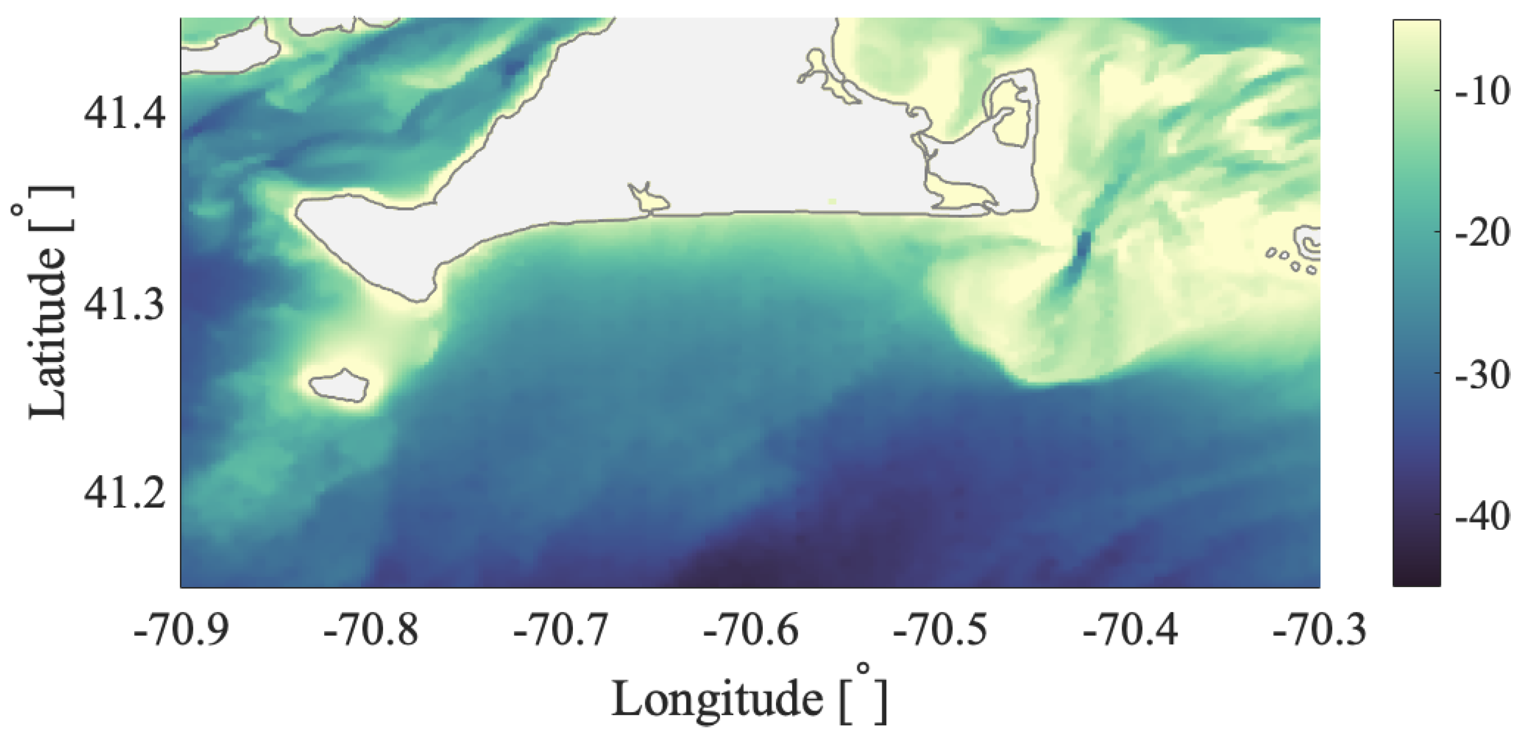
Our specific area of interest was the region around a small uninhabited No Man’s Land island located approximately 5 km south of the western end of Martha’s Vineyard (Figure 6). The depth of the channel between Martha’s Vineyard and No Man’s Land is about 10 m on average, with steep gradient on each side. East and west of No Man’s Land, the depths increase to 25 m over a few kilometers. The flow south of Martha’s Vineyard is strongly affected by wind and tides [37,38].
The drifters used in our study were the same as in [37], i.e., the Coastal Dynamics Experiment (CODE) type, also called Davis type, developed by [39] and manufactured by metOcean telematics. The model used was the primitive equation Multidisciplinary Simulation, Estimation, and Assimilation Systems (MSEAS) model developed at MIT [40,41]. MSEAS was configured with a two-way nesting: the domain around the continental shelf had a 600-m resolution and the domain around Martha’s Vineyard had a 200-m resolution. The model was forced by the atmospheric NCEP flux forecasts and tidal forcing from the Oregon State University barotropic tide model adapted to the bathymetry around Martha’s Vineyard. MSEAS was initialized with historical data from the National Marine Fisheries Service (NMFS) for conductivity, temperature and depth (CTD), and the sea surface temperature data provided by the Johns Hopkins University’s Applied Physics Lab (JHU APL). About a week prior to each field experiment, hydrographic surveys were conducted in the area of interest south of Martha’s Vineyard, and the collected CTD measurements were used to adjust the model boundary conditions with the observed ocean conditions. Details about surface forcing, and initial and boundary conditions for these runs can be found on the MSEAS website http://mseas.mit.edu/Sea_exercises/NSF_ALPHA.
MSEAS was re-run in a hindcast mode using the observed NCEP reanalysis wind forcing (instead of forecasted winds) after the end of the field experiments. The hindcast runs are qualitatively similar to the forecast runs in all respects. Quantitatively, MSEAS hindcasts for both 2017 and 2018 generally agree better with the observed real drifter motion than the forecasts, although the short-term strong-wind events (discussed in more detail below) that occurred during the 2018 field experiment and that were not well-represented by the NCEP reanalysis, led to the poorer agreement between model and drifters in 2018 compared to the 2017 experiment. For brevity, in this paper we only present the analyses of the MSEAS hindcasts, but the forecast-based results obtained in real time during the field experiments are qualitatively similar.
For ease and speed of Lagrangian calculations, the TRACE web-based gateway [42] (http://transport.me.berkeley.edu/thredds/catalog/public/MIT-MSEAS/catalog.html) was used to compute trajectories of simulated drifters advected by MSEAS currents, as well as the FTLE fields. The trajectory integration time in this study was 6 h, which is an important timescale for a flow with a strong M2 tidal component, and also represents the upper time limit in the real person-lost-at-sea search-and-rescue operations.
3.3.1. 2017 Experiment
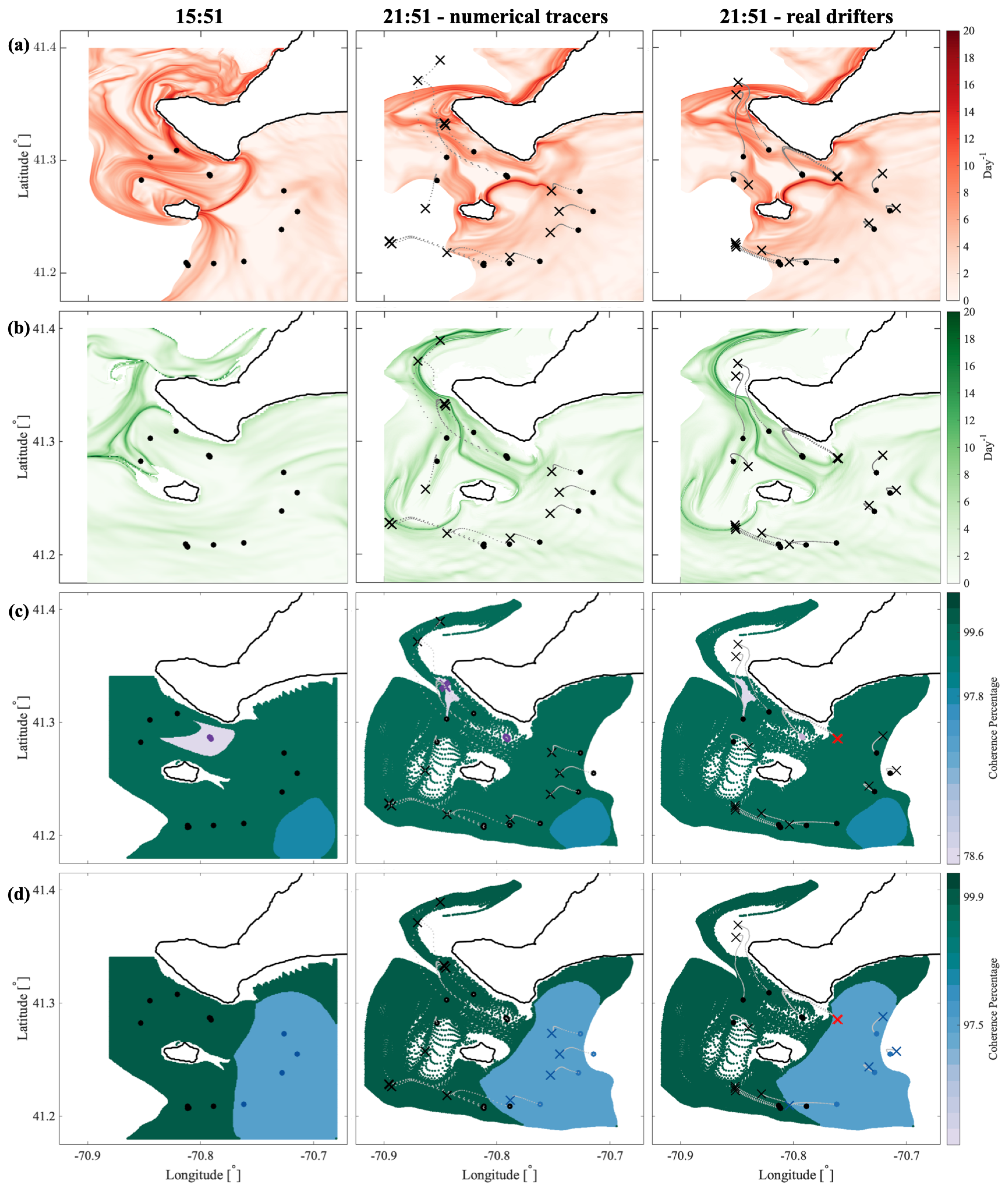
On 14 August 2017, we released 14 drifters at 10 locations (i.e., triplets were released at 2 locations—station #4 from the west and the southernmost station in Figure 7a) in a circumvent pattern around No Man’s Land. Deployment took 1.5 h, with the last drifter hitting water at 15:51. The deployment strategy targeted different coherent regions delineated by the separating LCSs. The 360-degree circumvent pattern around the island ensured that drifters would be deployed on opposite sides of any LCS that protrudes from any point on the island in any direction, thus mitigating uncertainties in the exact positions of model-based LCSs. Figure 7 shows the drifter deployment locations and 6-h long drifter trajectories, as well as the forward- and backward-FTLE fields and the coherent clusters identified using the optimized-parameter spectral clustering method.
For a unidirectional flow that impinges on an island from any direction, a hyperbolic trajectory is expected to form on the side of the island facing the inflow and on the opposite side facing the outflow. From the former hyperbolic trajectory, a stable manifold is expected to protrude into the incoming flow, separating trajectories passing the island on opposite sides. The real oceanic flow is not unidirectional and, with a strong tidal component, changes significantly over the 6-h analysis window. Nevertheless, consistent with the expectations described above, forward FTLEs show a strong repelling ridge extending from No Man’s Land across the eastern side of the channel toward Martha’s Vineyard (Figure 7a). (Some indication of multiple backward-FTLE ridges is also seen on the western side of the No Man’s Land (Figure 7b) but these are not as strong as the above-mentioned forward FTLE ridge.) As we go from west to east across the red forward FTLE ridge in Figure 7a, 4 deployment locations (black dots) lie to the west of it and 3 to the east, with the remaining 3 deployment locations further away from it on the southern side of the island. The drifters on opposite sides of this ridge are expected to have qualitatively different Lagrangian motion, and indeed, trajectories of the three drifters on the eastern side of this repelling ridge are significantly different from the rest in that they barely move over the subsequent 6 h and are by far the shortest. This is also consistent with the smaller FTLE values in this region (fainter red) indicating a more quiescent character of the flow. Multiple additional forward FTLE ridges are seen west and north of the No Man’s Land, which lead to the complicated behavior of drifters in this quadrant. Specifically, out of the 6 drifters deployed there, the westernmost drifter did not move much, the 2 northernmost drifters strayed far north, and the easternmost triplet of drifters looped around and came back.
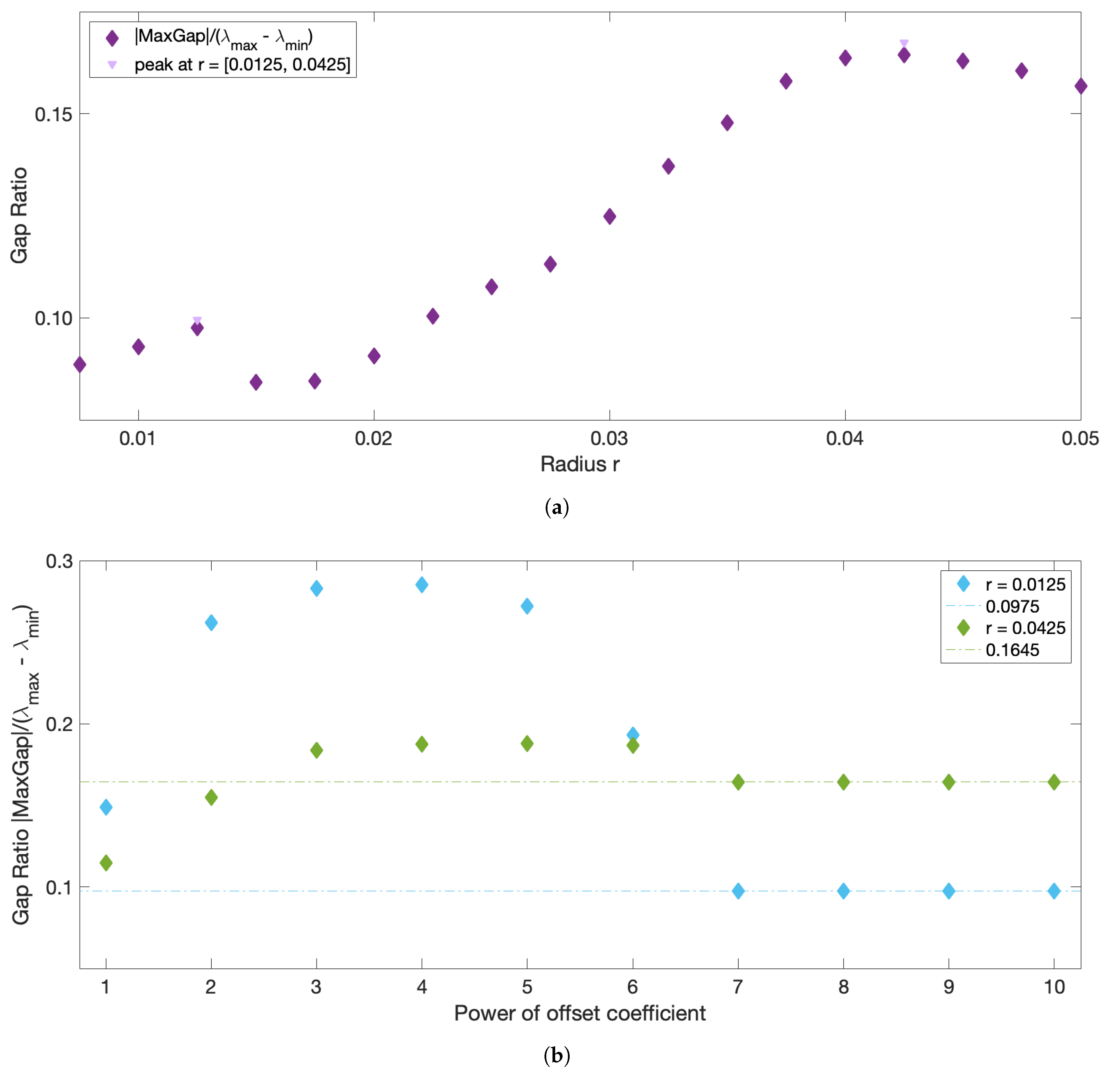
The coherent clusters obtained using the optimized-parameter spectral clustering method are shown in Figure 7c,d. The sweep with increasing r (Figure A3 in Appendix A.3) revealed 2 peaks in the normalized eigengap—at 0.0125 and 0.0425 deg (1.4 and 4.7 km). With respect to the offset, convergence in normalized eigengap was again achieved at for all r. The first peak at km yielded two coherent clusters: a less coherent purple one (78.6% coherence metric) located in the dynamically active region inside the channel, and a more coherent blue one (97.8% coherence metric) in the most quiescent southeastern corner of the domain; the rest of the domain was assigned to the green incoherent background (which was in fact very coherent with >99% coherence metric). The purple cluster is roughly delineated by the 2 forward FTLE ridges—a stronger one on the east and a weaker one on the west. When advected forward in time for 6 h, the purple cluster moves northward and shrinks in area, suggesting that convergence of the surface flow could be an important physical mechanism responsible for the existence of this coherent cluster. The second peak, at km, yielded one large coherent cluster (97.5% coherence) occupying most of the quiescent eastern part of the domain, with the rest of the domain assigned to the incoherent background (again with >99% coherence).
Comparing the motion of real drifters against the model-based spectral clusters, the purple cluster in the channel did not hold the triplet of drifters that were released there. After initially heading northwest with the shrinking purple cluster, all 3 drifters looped around and headed back southeast, ending up in the green incoherent background not far from their release location after 6 h. This is most likely due to a combination of the uncertainties in the numerically simulated ocean currents (see Figure A10 in Appendix C.1 for the differences between the real and simulated drifters), the most dynamic character of the flow in this region with high sensitivity to the drifters deployment locations, and the fact that the purple cluster was the least coherent out of all clusters (only 78% coherent) and thus is most sensitive to noise. All other drifters were deployed in the green region in Figure 7c, and all stayed there after 6 h. With respect to the clusters in Figure 7d, 4 drifters were released within the blue coherent cluster and all 4 stayed there. The rest of the drifters were deployed in the green background region; 7 stayed there, whereas one triplet switched from green to blue.
3.3.2. 2018 Experiment
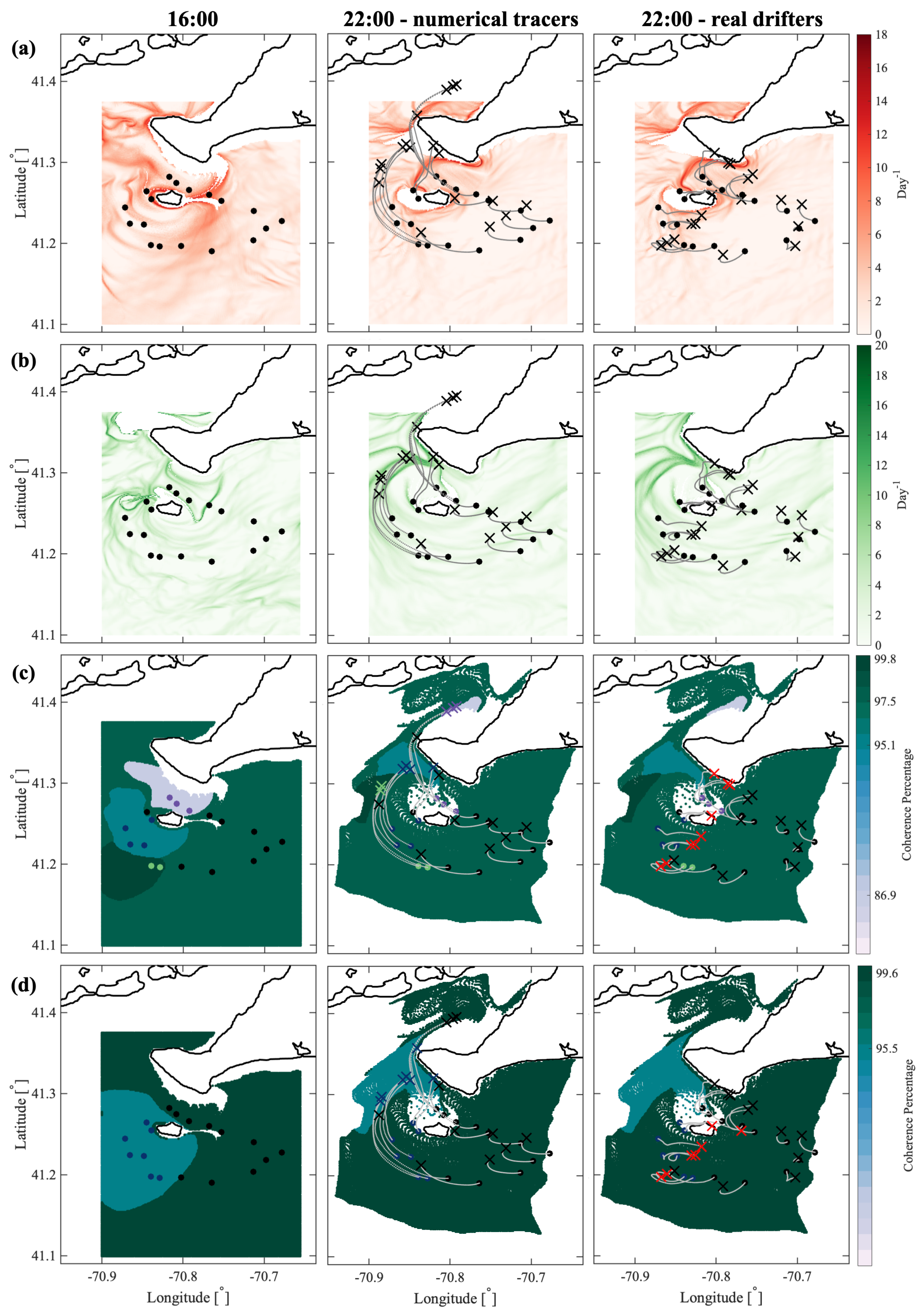
The 2018 No Man’s Land experiment took place on 7 August. A similar circumvent deployment route around No Man’s Land was used, but with 18 drifters, instead of 14 as in 2017. The deployment was completed at 16:00 so that over the subsequent 6 h the drifters would sample the same part of the tidal cycle as in 2017.
Intermittent eastward wind gusts of up to 25 m/s started to occur shortly after the drifter deployment, from 16:00 until 20:00. (Measured wind time series for the Martha’s Vineyard Airport station for 7/8/2018 can be found on The Weather Underground website). These wind gusts were absent in the NCEP wind forecasts and the corresponding MSEAS model forecasts, and were under-represented in the NCEP hindcast wind reanalysis (due to temporal intermittency and spatial variation of winds around Martha’s Vineyard and No Man’s Land) and the corresponding MSEAS hindcast currents. The wind gusts strongly affected the drifter trajectories, caused beaching of 2 drifters, and led to the generally poor agreement between the real and simulated drifter trajectories over the first 6 h of the experiment (Figure A11 in Appendix C.2). Agreement between the real and simulated drifters had improved after the end of the wind gust period (Figure A12), but the 6-h time interval from 20:00 on August 7 until 02:00 on August 8 corresponds to a different part of the tidal cycle and thus cannot be directly compared to the 2017 results. Analysis of the same tidal phase of the next tidal cycle, i.e., 04:00–10:00 on August 8, is possible but by then all drifters had moved east of No Man’s Land (Figure A13), and the initial elliptical deployment pattern had been distorted into a geometrical configuration that was sub-optimal for testing the agreement with spectral clusters. Thus, the comparison of the 2018 spectral clusters with real drifters and with the results from the 2017 experiment is challenging, no matter what time window is chosen. Here, we present the analysis for 3 different time windows, and we learn something from each.
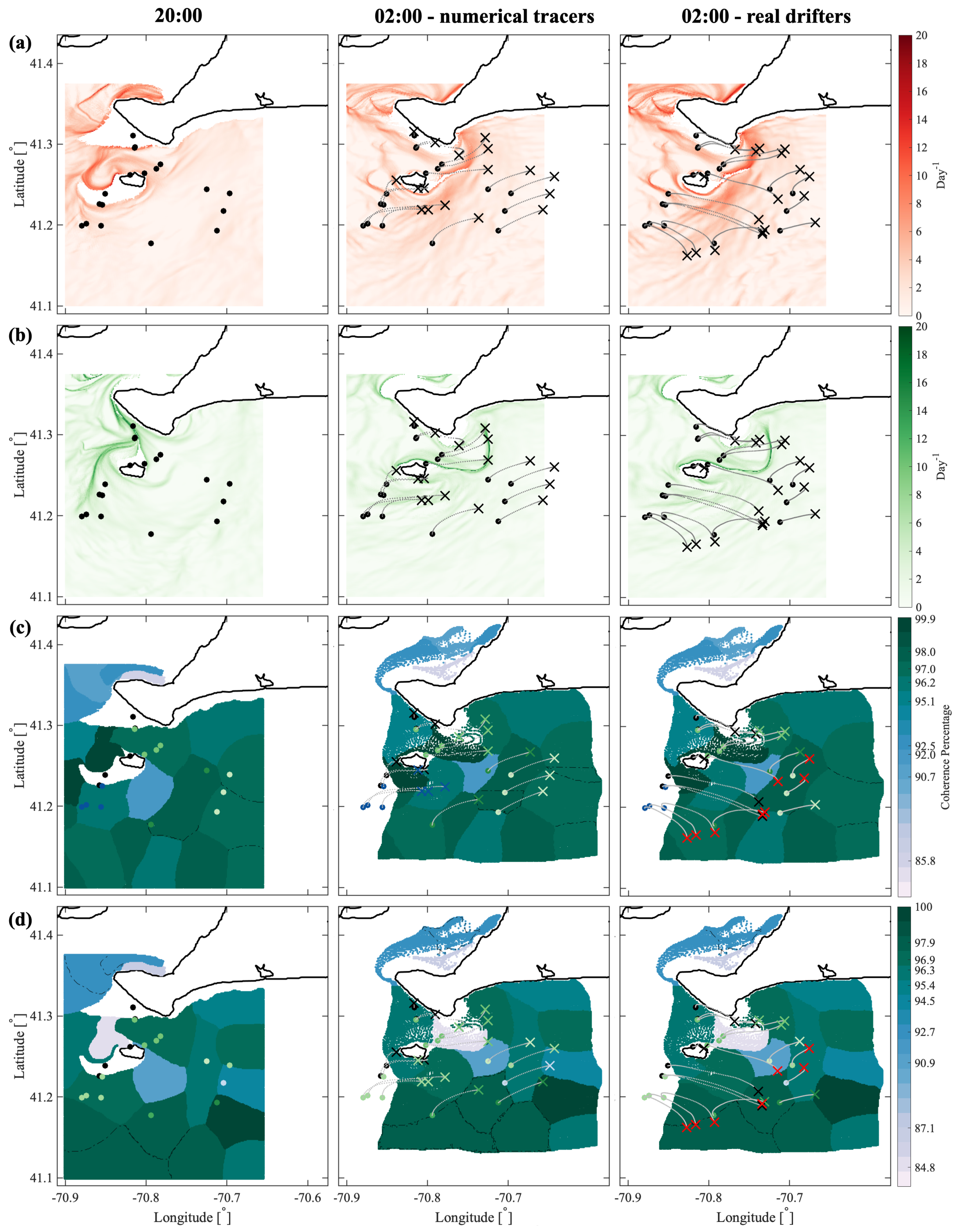
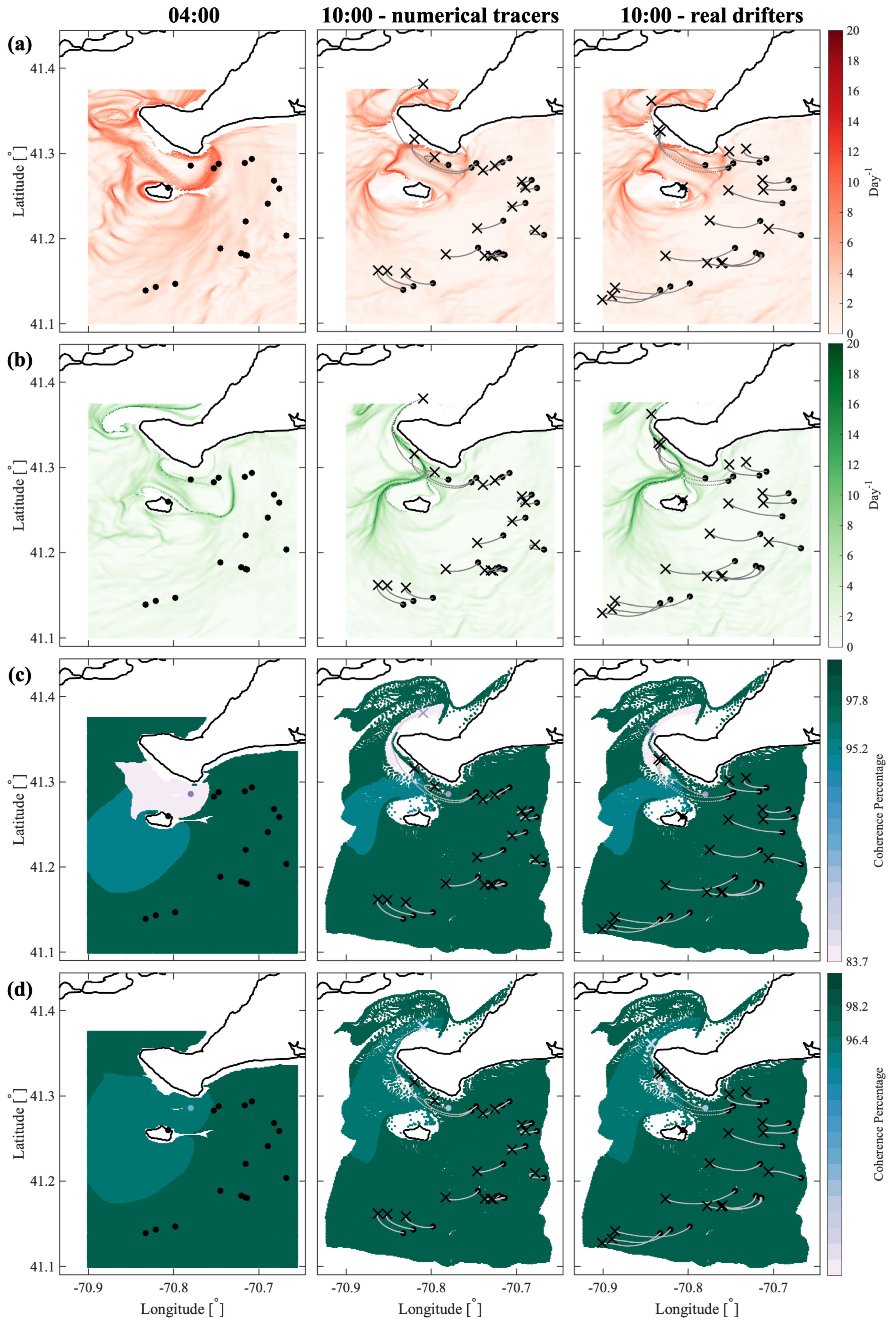
The results for the 3 different 6-h time windows, 16:00–22:00 on 7 August; 20:00 on 7 August—02:00 on 8 August; and 04:00–10:00 on 8 August, are presented in Figure 8, Figure 9 and Figure 10. The format of each figure is akin to the 2017 results in Figure 7: left and right panels correspond to the start and end of each time window, the top two rows show forward and backward FTLEs, and the bottom rows show spectral clusters.
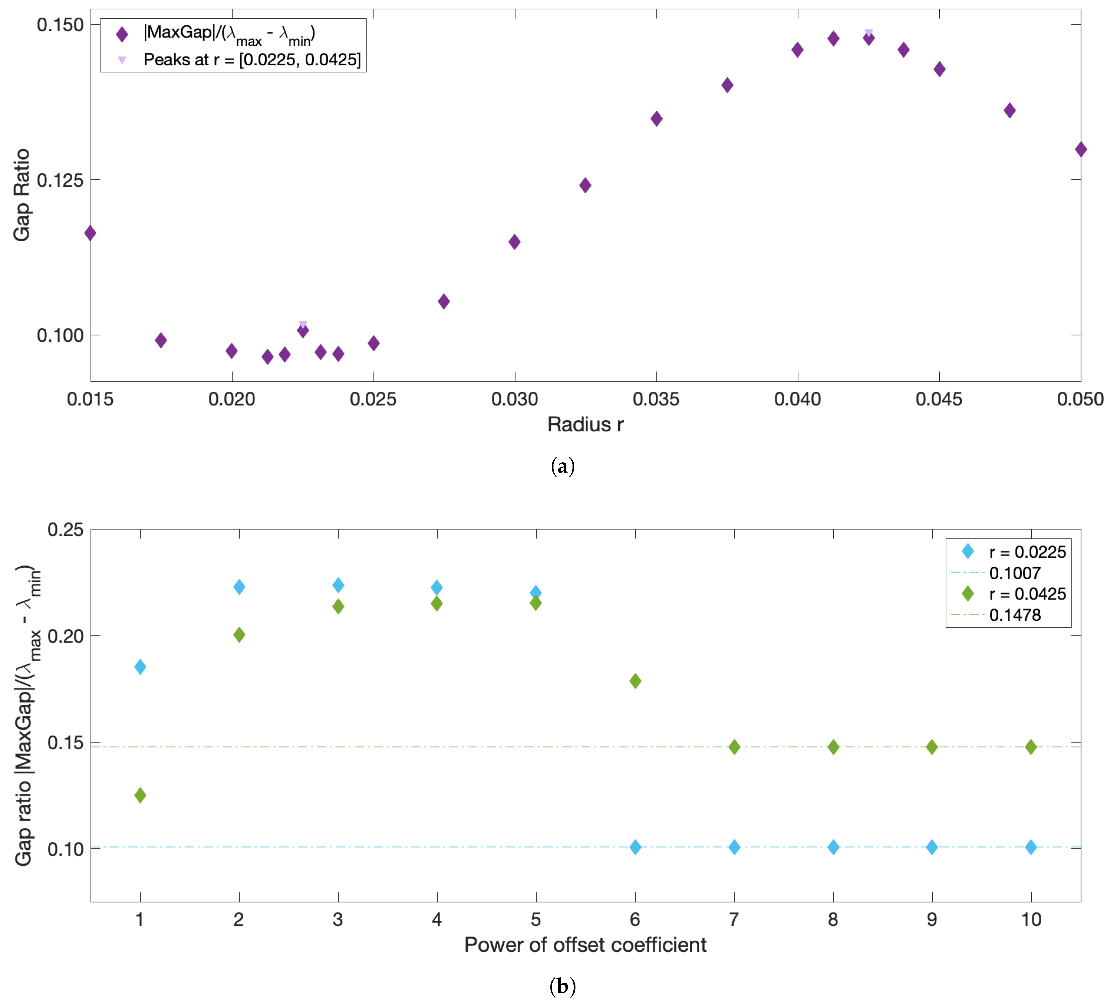
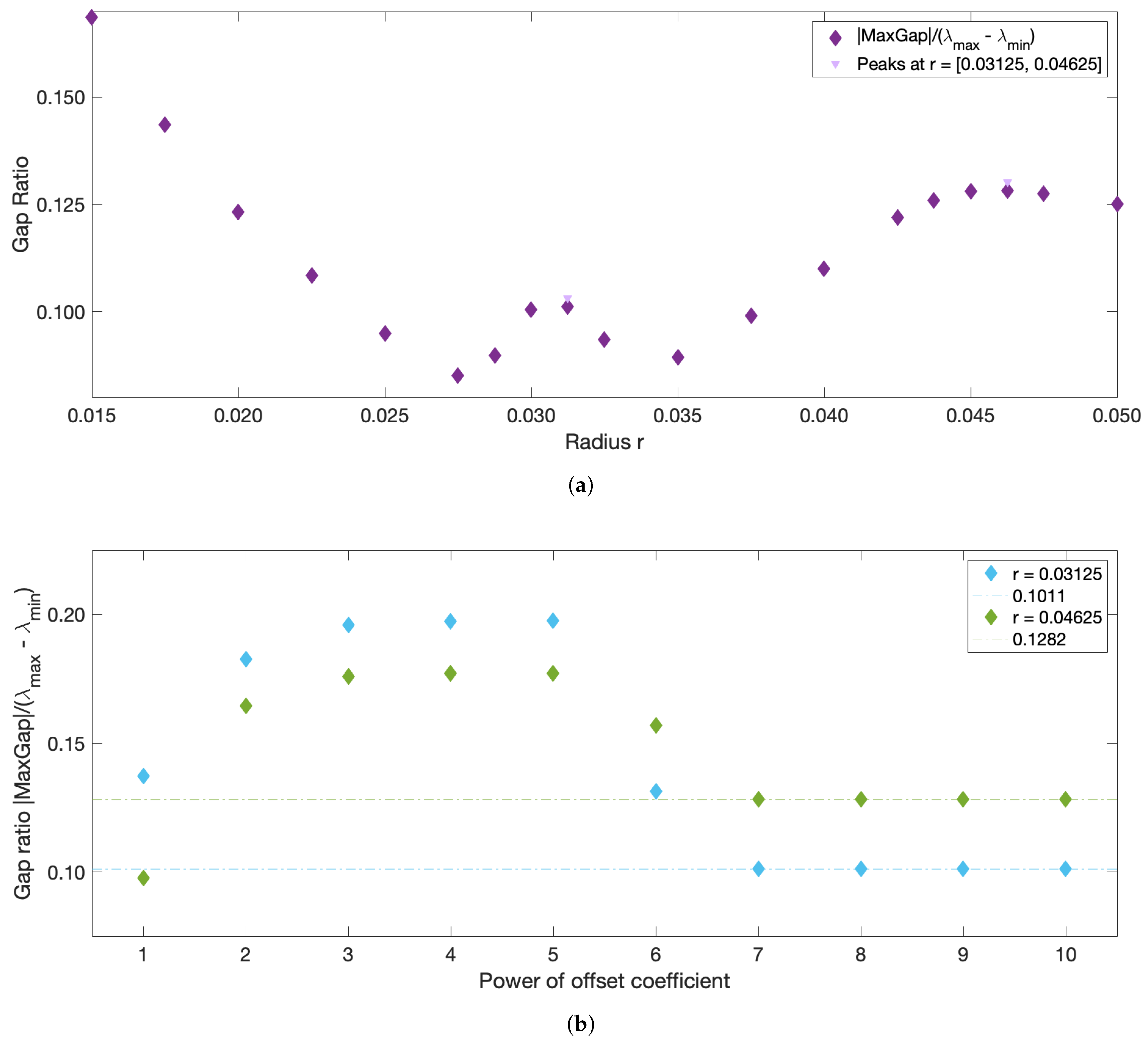
For the 16:00–22:00 and 04:00–10:00 time windows (Figure 8 and Figure 10), the FTLE fields are qualitatively similar to each other and, in many respects, to those from 2017 (Figure 7). A strong repelling forward FTLE ridge is seen extending from No Man’s Land to Martha’s Vineyard across the eastern part of the channel (panel a-left). Additional ridges and the overall elevated FTLE values are seen in the northwestern quadrant of the domain, reflecting on the complex Lagrangian behavior and strong sensitivity to deployment locations in this region. The opposite southeastward quadrant shows the smallest FTLEs indicative of the more quiescent character of the flow with lesser drifter separation. For this tidal phase in 2018, similar to 2017, the optimized-parameter spectral clustering results have 2 peaks (at for 16:00–22:00 and for 04:00–10:00, with convergence in w at the same coefficient as in all other examples—see supplementary Figure A4, Figure A5 and Figure A6).
At 16:00, the first peak revealed 3 clusters: a cluster in the channel and two clusters to the south-southwest of No Man’s (Figure 8). The channel cluster is qualitatively similar to the 2017 purple cluster. The rest of the domain is assigned to the green around-cluster background. When advected forward over 6 h, the clusters to the south-southwest of No Man’s Land moves anticyclonically around the island and into the channel, whereas the purple channel cluster moves northward, hugging the tip of Martha’s Vineyard and shrinking in size, which is again qualitatively similar to 2017. The second peak revealed a large cluster in the center-eastern part of the domain that encompasses the dark green and turquoise coherent clusters from the first peak, No Man’s Land and parts of the purple cluster. Comparing the spectral clusters for the 16:00–22:00 time window against real drifters, the agreement is poor as all drifters released within a cluster ended up in the incoherent background, very likely due to the unresolved wind gusts in the model.
The 04:00–10:00 time window (Figure 8) corresponded to a similar phase of the tidal cycle and each peak in r yielded results that had many qualitative similarities to the 16:00–22:00 time window. The first peak again revealed a purple channel cluster and a second, turquoise, cluster south of No Man’s Land. After 6 h, the channel cluster moves northward around Martha’s Vineyard and the turquoise cluster moves anticyclonically around No Man’s Land and into the channel. The second peak revealed a large, highly coherent cluster shown in dark teal that encompasses parts of both clusters from the first peak. In both cases, l7 drifters were initially located in the green inter-cluster background and 1 drifter started in the channel, in the purple cluster in (c) and the dark teal cluster in (d). All drifters stayed within their respective cluster, but since only 1 drifter was initially inside the purple cluster, the comparison might not be statistically robust.
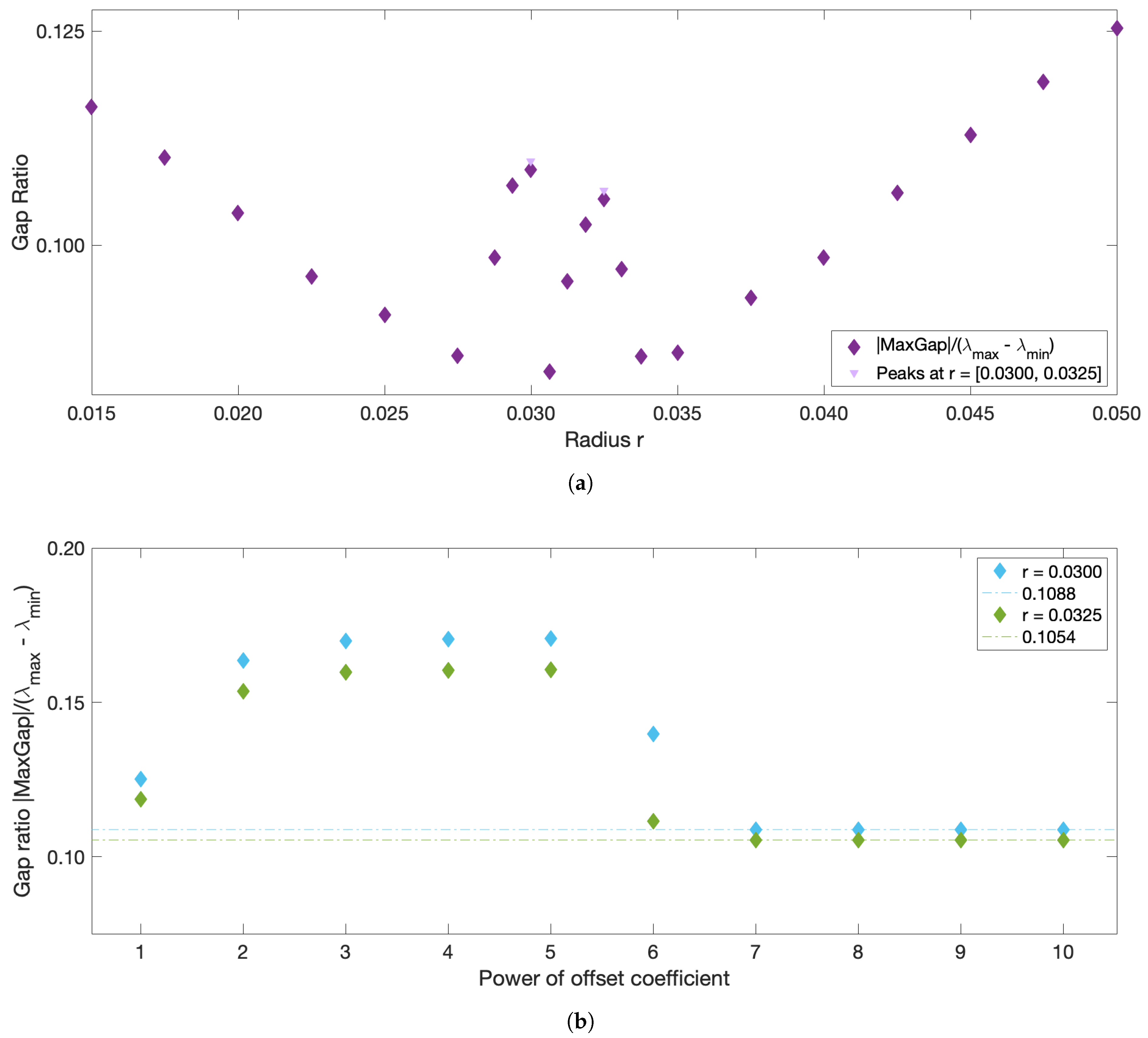
Looking at the result over the different phase of the tide, from 20:00 to 04:00 UTC in Figure 9, we see a qualitatively different geometry both in the FTLE fields and spectral clusters. The optimized-parameter spectral clustering has 2 peaks in the normalized eigengap—at . Both have very large number of clusters (17 and 18, respectively), and both do not identify the inter-cluster background. This large number of clusters suggests that over this tidal period, no part of the domain is significantly different from the rest of the domain in terms of Lagrangian connectivity, unlike in all 3 other Martha’s Vineyard cases that consistently show 1 to 3 coherent clusters embedded into the inter-cluster background. For the 20:00–04:00 time window, the comparison with real drifters showed mixed results. The four drifters released within the channel clusters in Figure 9a–d stayed within their assigned channel clusters, but otherwise, about half of the drifters left their assigned clusters by 04:00.
4. Discussion
A reliable method for identifying coherent clusters in oceanic flows is important for a variety of applications – from understanding of mixing and exchanges of biogeophysical tracers, to hazard mitigation and search-and-rescue operations. In studies of exchange processes, coherent clusters can help visualizing tracers that stay coherent over time. In hazard mitigation applications, clusters are useful for identifying areas where mitigation assets should be focused, and in the search-and-rescue operations, cluster geometries help narrow down on the optimal search-and-rescue pattern. The conventional spectral clustering algorithm has many of the desired qualities, yielding clusters that maximize inter-cluster similarity and intra-cluster differences of the underlying Lagrangian motion. Spectral clustering also has advantages over other techniques for LCS identification, such as FTLEs, in applications with sparse Lagrangian data. The major drawback of the conventional spectral clustering is the need for subjective user-defined choices for several method parameters, which requires a priori knowledge about the flow. The parameter choices vary between different flows and depend on flow characteristics such as intensity, spatial variability, and dominant spatio-temporal scales of the currents, which might not be known in real applications. Different parameter choices generally yield substantially different coherent clusters, which drastically complicates the applicability of this method.
In this paper, we describe a new optimized-parameter spectral clustering algorithm, which automatically identifies optimal parameters within pre-defined parameter ranges for a given flow(the pre-defined parameter range and the parameter increment for the sweeps still need to be specified by the user). The specific parameters of interest are the sparsification radius r, which is responsible for the sizes of the identified clusters, and the offset parameter , which is responsible for the numerical stability of the algorithm. Automated selection of optimal r and requires modifications of the conventional spectral clustering. Specifically, we introduce a normalized spectral eigengap, which allows inter-comparison between different r-choices, instead of the absolute eigengap used in the conventional method, which typically decreases with r. (As in the conventional spectral clustering, the optimal number of clusters is defined as the number of eigenvalues before the eigengap.) The optimal r value(s) is then identified as the value(s) that corresponds to the local maximum (or maxima) of the normalized eigengap. Specifying r in this manner ensures that for clusters of that particular size the inter-/intra-cluster similarity is largest/smallest compared to clusters that are either smaller and larger. Since many geophysical flows operate on multiple spatio-temporal scales, clusters of very different sizes could simultaneously exist within the same flow, and looking at all peaks in r ensures that we identify all of them. The second method parameter, , is chosen as the smallest at which convergence of the normalized eigengap is achieved. Finally, to evaluate the coherence of the clusters, we introduce a noise-based coherence metric that allows comparing clusters within the same flow or between different flows. This metric quantifies the relative robustness of the resulting clusters with respect to applied numerical noise.
The automatic detection of multi-scale features is a well-known problem for conventional graph cut methods, including the normalized cut (which lies at the core of the spectral clustering) that favors clusters of equal size [30]. When clusters are well separated from each other and their sizes are only slightly different, such as in the periodically forced pendulum example in HA16 or in our slightly asymmetric oscillator example, all clusters can be identified using a single r value. However, when the clusters are sufficiently different in size, such as in our strongly asymmetric Duffing oscillator example, different r values are needed to correctly identify all the coherent sets. Thus, in general, no single r can be guaranteed to identify all the clusters. By doing sweeps in r and identifying all the r values that correspond to the local maxima in the normalized eigengaps, we can overcome this challenge and identify all the underlying coherent sets across a wide range of spatial scales. This is particularly important in oceanic applications, in which very little is known a priori about the flow and the scales of the coherent features. Oceanic flows often have more than one dominant length scale, and thus, multiple coherent clusters with different sizes may coexist within the same flow. This was indeed the case for the coastal flow south of Martha’s Vineyard. In all our oceanic examples, the optimized-parameter spectral clustering algorithm identified 2 optimal values of the sparsification radius, r, yielding 2 different partitions of the domain into coherent clusters with different sizes.
The optimized set of parameters, as well as the specific noise-based metric of coherence that we have proposed here, present one possible way to reduce the user-input parameter choices and quantify the coherence of the resulting clusters. We explained the logical arguments underlying our proposed optimized-parameter algorithm, and we illustrated that our method reliably yields parameters and clusters that are optimal according to our specific definition. The strength of our optimized-parameter spectral clustering method is that it allows applying the method to any flow with minimal prior knowledge about it, and that the method automatically identifies clusters with minimal user input, along with a coherence value for each cluster.
Although optimized-parameter spectral clustering requires less user input than the conventional spectral clustering of HA16, we cannot claim that our method is completely parameter-free. Being of spectral nature, our optimized-parameter spectral clustering is also subject to all the limitations typical of other spectral methods. In our approach, the user still needs to specify the upper and lower limits for the parameter range, as well as the increment in the parameter values for the sweep. The method will then automatically identify the optimal parameters, detect the clusters and quantify their coherence. Since less information is needed for specifying the parameter range than specifying the exact parameter value, our method is easier to use in applications to the largely unknown oceanic flows, and it comes one step closer towards a parameter-free coherent structure identification.
We have tested the optimized-parameter spectral clustering in 2 commonly used benchmark analytic flows—Bickley Jet and Duffing oscillator—and in a real-life oceanic application to a high-resolution model-based surface flow in the coastal region south of Martha’s Vineyard, MA. The results are encouraging in that our method identified all known coherent clusters in both benchmark flows, and it identified reasonably looking clusters in the realistic oceanic example. Looking at the coherence of the clusters and the optimality of the resulting partition of the domain, both analytic flows had significantly larger values of normalized eigengaps (0.4–0.5) than the real oceanic flows (about 0.1), pointing to the poorer performance of the method in the latter examples. This is not surprising as both analytic flows have a stronger contrast in Lagrangian behavior between the coherent regions associated with the (more regular) gyre cores and the incoherent background that encompasses the well-mixed (chaotic) regions around the gyres, whereas in the realistic oceanic flows, this contrast between regular and chaotic motion is smeared. In all examples, however, our method still yielded clusters with relatively high values of noise-based coherence (above ), suggesting that even for the flow south of Martha’s Vineyard, the detected clusters were robust features of the flow that are not excessively sensitive to numerical noise and observational and model uncertainty. For the 2018 campaign, the 20:00–02:00 experiment exhibited particularly low gap ratios and the domain partitions were far from optimal, with numerous (≥17), small clusters adjacent to each other and an incoherent cluster that was indistinguishable from the coherent ones. This illustrates the limits of the method’s applicability: although the method did produce a partition into clusters, the flows need a certain amount of dissimilarity for the resulting clusters to be meaningful. This is discussed in HA16 and their notion of coherence, which exists in the presence of an incoherent background.
In the Martha’s Vineyard case study, since the flow south of the Vineyard has a strong tidal component, the resulting coherent clusters are qualitatively similar over the same phase of the tide on different days and even different years, whereas coherent clusters for the opposite tidal phase are qualitatively different. The strong dependence of the cluster geometry on the tidal phase has been also observed in tidally driven flow over an experiment in Scott Reef, Australia [43]. Comparing the model-based clusters south of Martha’s Vineyard to the motion of real drifters, for most of the identified clusters, drifters deployed within a cluster stayed within the same cluster for 6 h, which was the time interval chosen for our analysis. Exceptions, i.e., clusters from which real drifters escaped in less than 6 h, include small clusters with lower coherence metric or clusters identified over the time interval with strong wind gusts that were not realistically represented in the numerical model of oceanic currents.
Comparing coherent clusters with FTLE fields reveals that cluster boundaries often have similarities with the forward-time FTLE ridges. This qualitative similarity is due to the repelling character of the forward FTLE ridges, which maximize separations between neighboring drifters and delineate regions of qualitatively different Lagrangian motion. In other cases, coherent clusters were identified in areas that shrink significantly over the subsequent 6 h, suggesting that these clusters might be dominated by the surface flow convergence. Finally, some of the coherent clusters were identified over the most quiescent regions with lowest FTLEs, which encompass groups of drifters that moved (and separated) less than others. Note, however, that because the spectral clustering method identifies clusters based on a specific criterion, i.e., by maximizing intra-/inter-cluster similarities/differences, one should not expect a one-to-one agreement between spectral clusters boundaries and FTLEs or other LCSs that use another underlying flow property. Thus, various complementary LCS techniques could be applied in concert to provide the most comprehensive view of the underlying Lagrangian transport.
Author Contributions
Conceptualization, M.F., I.I.R. and T.P.; methodology, M.F., A.H. and I.I.R.; software, M.F. and A.H.; validation, M.F.; investigation, M.F.; resources, I.I.R. and T.P.; data curation, M.F.; writing—original draft preparation, M.F.; visualization, M.F.; supervision, A.H., I.I.R. and T.P.; project administration, I.I.R. and T.P.; funding acquisition, I.I.R. and T.P. All authors contributed to the formal analysis and to the writing—review and editing. All authors have read and agreed to the published version of the manuscript.
Funding
M.F., I.I.R. and T.P., and the field studies, were supported by the U.S. National Science Foundation (NSF) under Grant Number AGS 1520825 (Hazards SEES: Advanced Lagrangian Methods for Prediction, Mitigation and Response to Environmental Flow Hazards). M.F. also acknowledges student support from the Woods Hole Oceanographic Institution. I.I.R. also acknowledges support from the NSF Grant # EAR-1520825.
Data Availability Statement
The data presented in this study are available on request from the corresponding author.
Acknowledgments
The authors acknowledge the contributions from the MSEAS team, who provided the ocean circulation models and the output numerical velocity fields, and Siavash Ameli for providing the TRACE web-based gateway. The authors thank the ALPHA project team for their help with field work.
Conflicts of Interest
The authors declare no conflict of interest.
Abbreviations
The following abbreviations are used in this manuscript:
| FTLE | Finite-Time Lyapunov Exponent |
| FCM | Fuzzy C-Means |
| LCS | Lagrangian Coherent Structure |
Appendix A. Verification of Parameter Convergence
Appendix A.1. Bickley Jet
Figure A1.
(a) Step 1 of the spectral clustering protocol for the Bickley Jet example: normalized eigengap as a function of r with the average distance function. (b) Step 2 of the spectral clustering protocol for the Bickley Jet: sweep of offset coefficients for the gap ratio peaks in (a) at , and with the average distance function.

Appendix A.2. Asymmetric Duffing Oscillator
Figure A2.
Steps 1 and 2 of the spectral clustering protocol for the asymmetric Duffing oscillator. (a) Sweep of r parameters with offset coefficient for the average distance function. (b) Sweep of offset coefficients for average distance function and the normalized eigengap peak at .
Figure A2.
Steps 1 and 2 of the spectral clustering protocol for the asymmetric Duffing oscillator. (a) Sweep of r parameters with offset coefficient for the average distance function. (b) Sweep of offset coefficients for average distance function and the normalized eigengap peak at .

Appendix A.3. 2017 No Man’s Land Experiment
Figure A3.
Steps 1 and 2 of the spectral clustering protocol for the 2017 No Man’s Land experiment for the 15:51–21:51 window. (a) Sweep of r parameters with offset coefficient for the average distance function. (b) Sweep of offset coefficients for average distance function and the normalized eigengap peaks in (a).

Appendix A.4. 2018 No Man’s Land Experiments
Figure A4.
Steps 1 and 2 of the spectral clustering protocol for the 2018 No Man’s Land 16:00–22:00 experiment. (a) Sweep of r parameters with offset coefficient for the average distance function. (b) Sweep of offset coefficients for average distance function and the normalized eigengap peaks from (a).

Figure A5.
Steps 1 and 2 of the spectral clustering protocol for the 2018 No Man’s Land 20:00–02:00 experiment. (a) Sweep of r parameters with offset coefficient for the average distance function. (b) Sweep of offset coefficients for average distance function and the normalized eigengap peaks from (a).

Figure A6.
Steps 1 and 2 of the spectral clustering protocol for the 2018 No Man’s Land 04:00–10:00 experiment. (a) Sweep of r parameters with offset coefficient for the average distance function. (b) Sweep of offset coefficients for average distance function and the normalized eigengap peaks from (a).

Appendix B. Duffing Oscillator with Increased Asymmetry
When the asymmetry of the Duffing oscillator is increased, such as in the example presented in Figure A7 the sizes of the left and right gyres become increasingly different from each other and no single r value can successfully identify both at the same time.
Figure A7.
Poincaré map for a second example of the asymmetric Duffing oscillator with 100 periods of perturbation T.
Figure A7.
Poincaré map for a second example of the asymmetric Duffing oscillator with 100 periods of perturbation T.

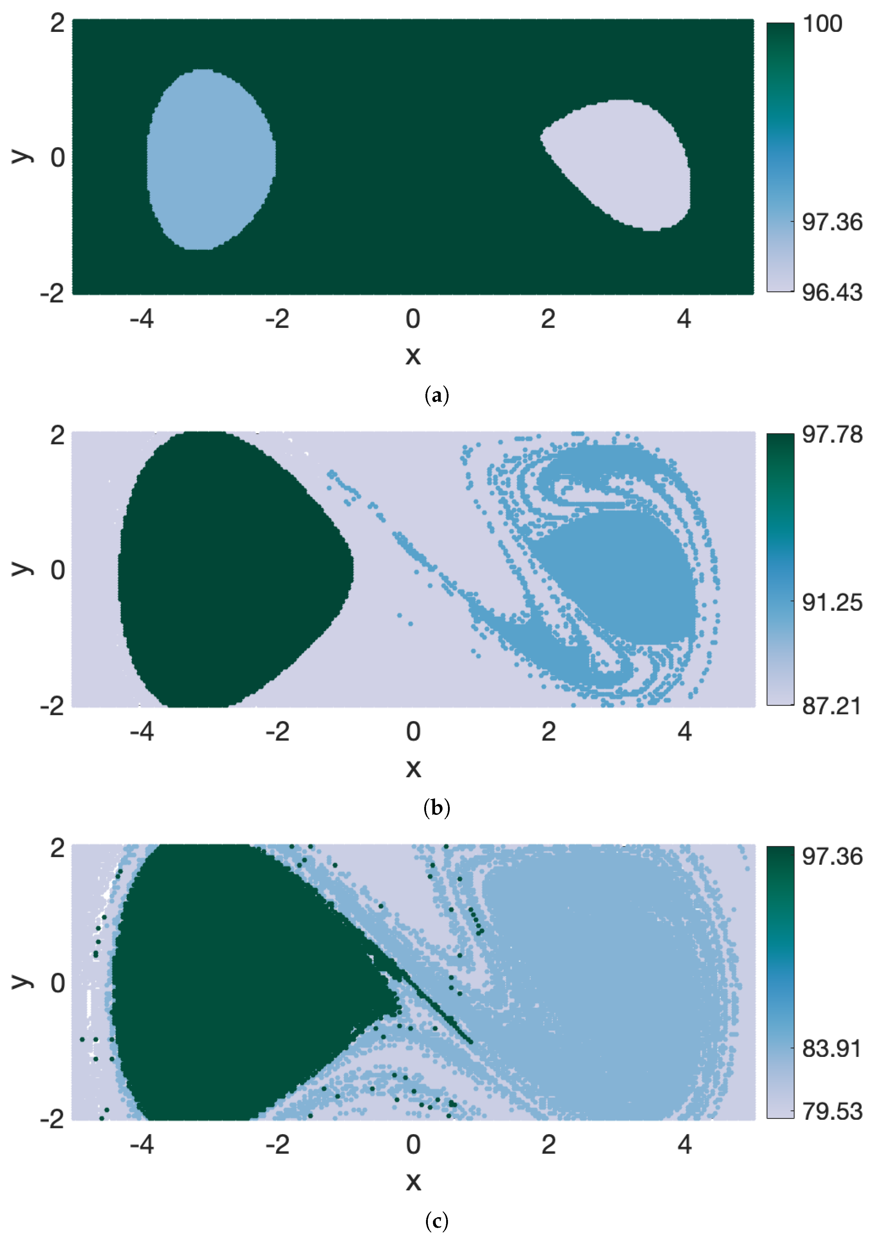
In this case, the r-sweep, shown in Figure A8, shows three local maxima in the normalized eigengap. The resulting coherent clusters, color-coded by their noise-based coherence metric are shown in Figure A9. Each peak in r shows 2 coherent clusters centered at the left and right gyres, and an incoherent background filling the space between and around them. The sizes of the clusters are different for different r (consistent with our interpretation of r as the parameter defining the size of the resulting clusters), as is the amount of cluster filamentation. The peak at the smallest correctly identifies the smaller right gyre, but pairs it with a left cluster that is smaller than the full extent of the left gyre. The peaks at correctly identifies the full extent of the larger left gyre, but pair it with a right cluster that is very filamented. The peak at the largest shows two clusters which are both too large and strongly filamented. The noise-based coherence metric can then be used to choose between the co-located clusters to pick one (out of three in this case) with the higher coherence, correctly yielding two clusters (the grey right cluster at and the green left cluster at ) corresponding to the full extent of the left and right gyres.
Figure A8.
Step 1 of the spectral clustering protocol for the asymmetric Duffing oscillator shown in Figure A7: sweep of r parameters with offset coefficient for the average distance function.
Figure A8.
Step 1 of the spectral clustering protocol for the asymmetric Duffing oscillator shown in Figure A7: sweep of r parameters with offset coefficient for the average distance function.

Figure A9.
Step 3 of the spectral clustering protocol for the asymmetric Duffing oscillator shown in Figure A7 for (a) , (b) and (c) . All individual clusters are color-coded by their coherence metrics.
Figure A9.
Step 3 of the spectral clustering protocol for the asymmetric Duffing oscillator shown in Figure A7 for (a) , (b) and (c) . All individual clusters are color-coded by their coherence metrics.

Appendix C. Comparisons between Real and Simulated Drifter Trajectories
Appendix C.1. 2017 No Man’s Land Experiment
Figure A10.
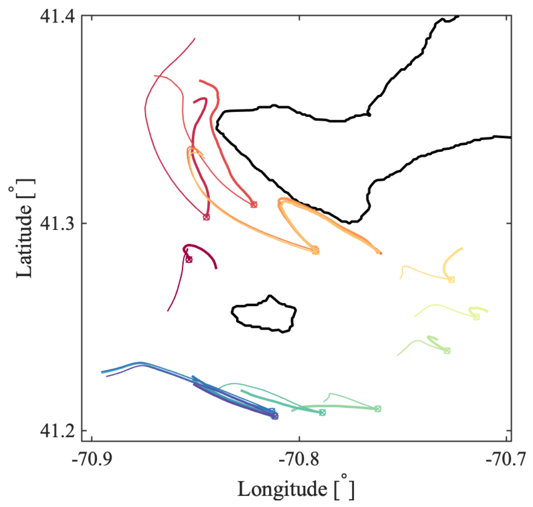
Comparison between real and simulated drifter trajectories for the 2017 No Man’s Land experiment. The trajectories of CODE drifters are plotted with thick lines. The corresponding numerical trajectories, simulated with the same initial conditions as their corresponding CODE drifter, are plotted with thin lines.
Figure A10.
Comparison between real and simulated drifter trajectories for the 2017 No Man’s Land experiment. The trajectories of CODE drifters are plotted with thick lines. The corresponding numerical trajectories, simulated with the same initial conditions as their corresponding CODE drifter, are plotted with thin lines.

Appendix C.2. 2018 No Man’s Land Experiments
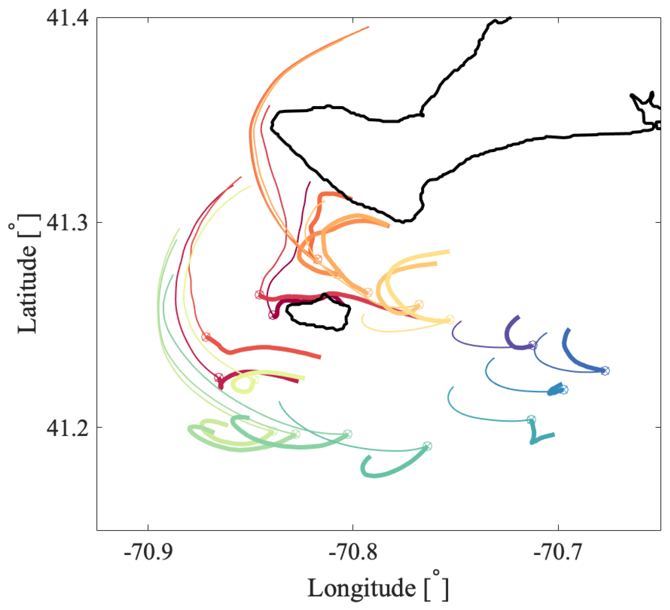
Figure A11.
Comparison between real and simulated drifter trajectories for the 2018 No Man’s Land experiment between 16:00 and 22:00 UTC. The trajectories of CODE drifters are plotted with thick lines. The corresponding numerical trajectories, simulated with the same initial conditions as their corresponding CODE drifter, are plotted with thin lines.

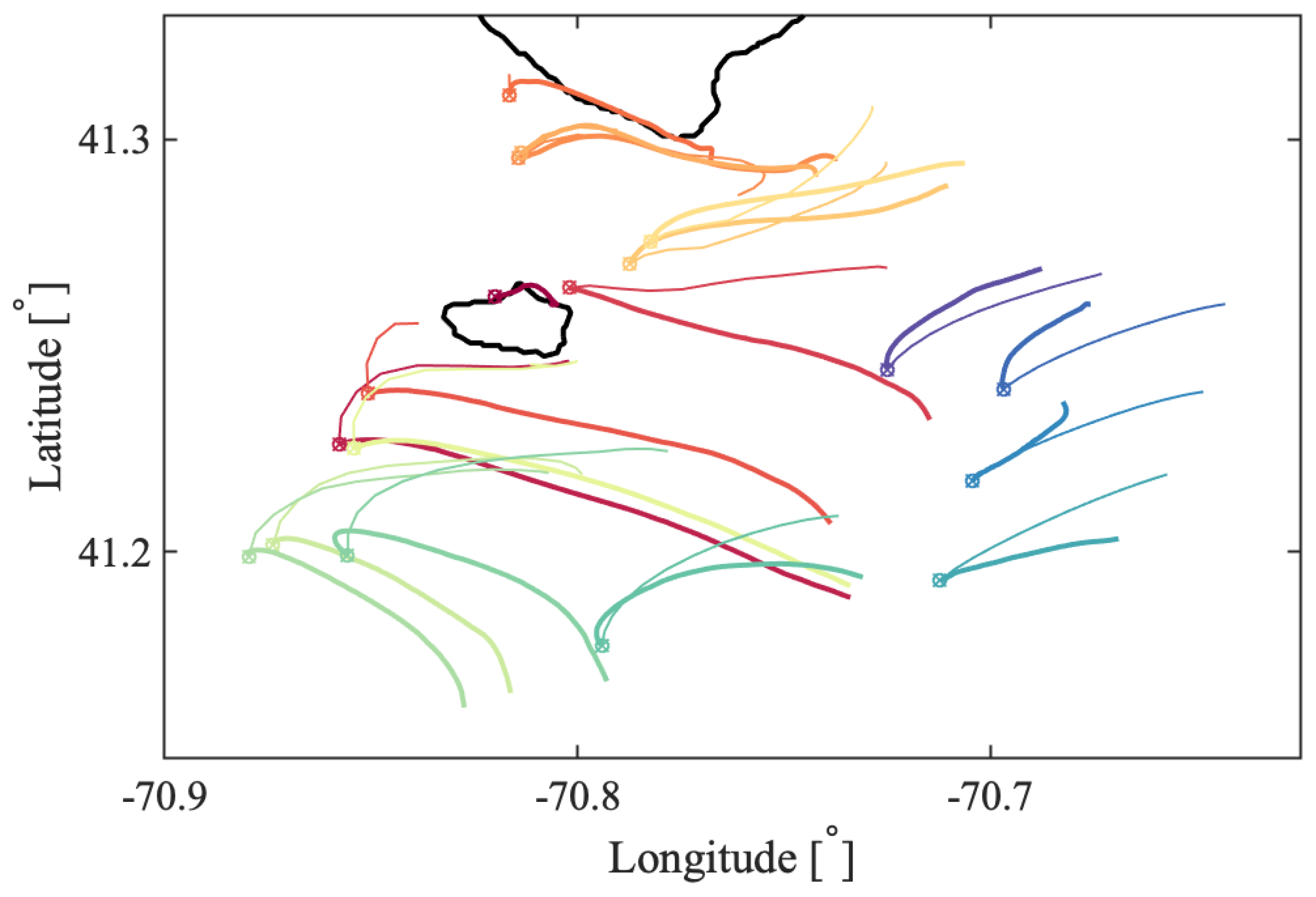
Figure A12.
Comparison between real and simulated drifter trajectories for the 2018 No Man’s Land experiment between 20:00 and 02:00 UTC. The trajectories of CODE drifters are plotted with thick lines. The corresponding numerical trajectories, simulated with the same initial conditions as their corresponding CODE drifter, are plotted with thin lines.

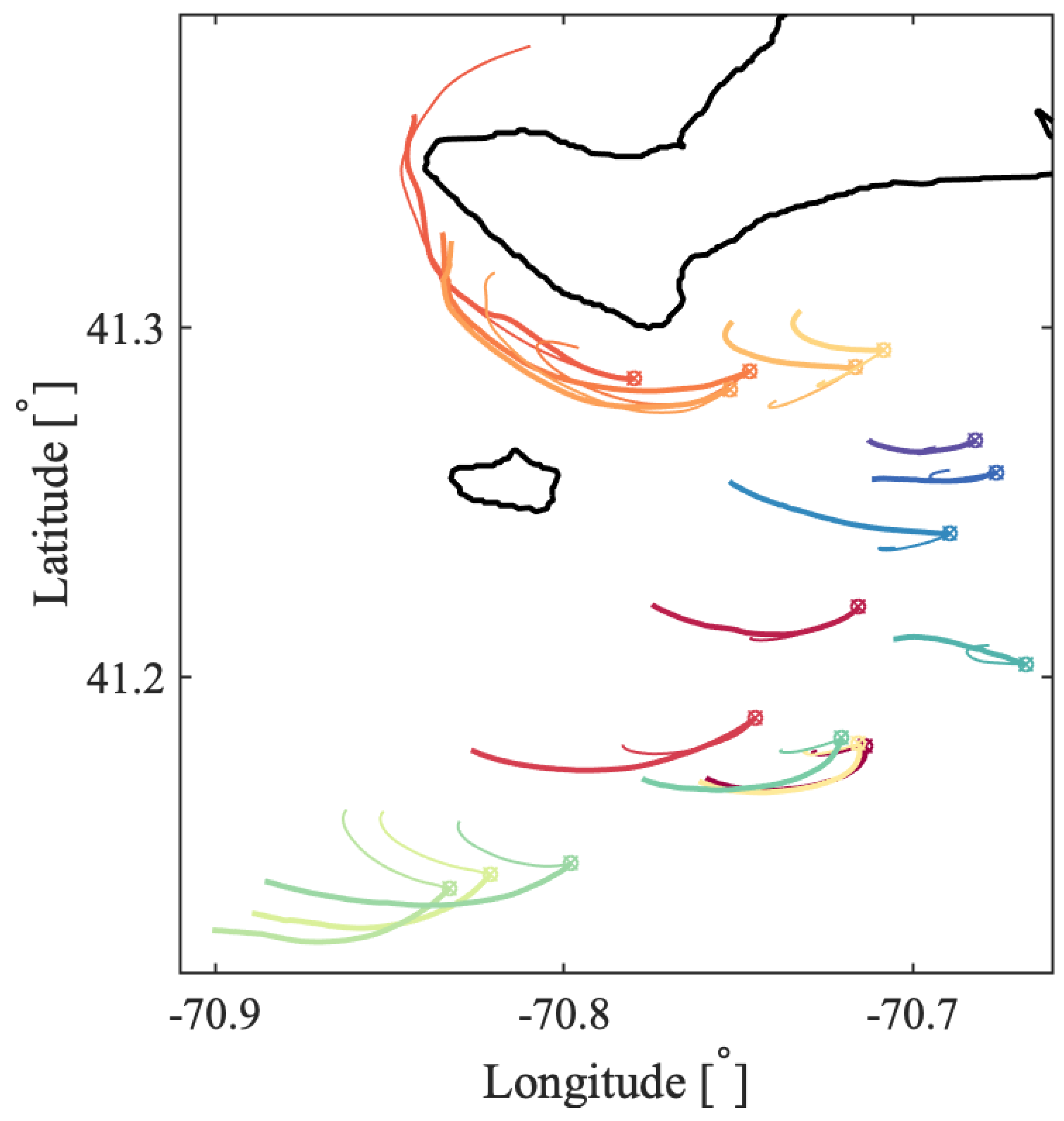
Figure A13.
Comparison between real and simulated drifter trajectories for the 2018 No Man’s Land experiment between 04:00 and 10:00 UTC. The trajectories of CODE drifters are plotted with thick lines. The corresponding numerical trajectories, simulated with the same initial conditions as their corresponding CODE drifter, are plotted with thin lines.

References
- Davis, R.E. Oceanic property transport, Lagrangian particle statistics, and their prediction. J. Mar. Res. 1983, 41, 163–194. [Google Scholar] [CrossRef]
- LaCasce, J.H. Statistics from Lagrangian observations. Prog. Oceanogr. 2008, 77, 1–29. [Google Scholar] [CrossRef]
- Rypina, I.I.; Pratt, L.J.; Pullen, J.; Levin, J.; Gordon, A.L. Chaotic Advection in an Archipelago. J. Phys. Oceanogr. 2010, 40, 1988–2006. [Google Scholar]
- Mendoza, C.; Mancho, A.M. The Lagrangian description of aperiodic flows: A case study of the Kuroshio Current. Nonlinear Process. Geophys. 2012, 4, 449–472. [Google Scholar] [CrossRef] [Green Version]
- Lehahn, Y.; d’Ovidio, F.; Koren, I. A Satellite-Based Lagrangian View on Phytoplankton Dynamics. Annu. Rev. Mar. Sci. 2018, 10, 99–119. [Google Scholar]
- Aref, H. Stirring by chaotic advection. J. Fluid Mech. 1984, 143, 1–21. [Google Scholar] [CrossRef]
- Rypina, I.I. Lagrangian Coherent Structures and Transport in Two-Dimensional Incompressible Flows with Oceanographic and Atmospheric Applications. Ph.D. Thesis, University of Miami, Coral Gables, FL, USA, 2007. [Google Scholar]
- Haller, G.; Yuan, G. Lagrangian coherent structures and mixing in two-dimensional turbulence. Phys. D Nonlinear Phenom. 2000, 147, 352–370. [Google Scholar] [CrossRef]
- Mathur, M.; Haller, G.; Peacock, T.; Ruppert-Felsot, J.E.; Swinney, H.L. Uncovering the Lagrangian Skeleton of Turbulence. Phys. Review Lett. 2007, 98, 144502. [Google Scholar] [CrossRef]
- Peacock, T.; Haller, G. Lagrangian coherent structures: The hidden skeleton of fluid flows. Phys. Today 2013, 66, 41–47. [Google Scholar]
- Villermaux, E. Mixing Versus Stirring. Annu. Rev. Fluid Mech. 2019, 51, 245–273. [Google Scholar]
- Wiggins, S. The dynamical system approach to Lagrangian transport in oceanic flows. Annu. Rev. Fluid Mech. 2005, 37, 295–328. [Google Scholar] [CrossRef] [Green Version]
- Allshouse, M.R.; Peacock, T. Lagrangian based methods for coherent structure detection. Chaos Interdiscip. J. Nonlinear Sci. 2015, 25, 097617. [Google Scholar] [CrossRef]
- Haller, G. Lagrangian Coherent Structures. Annu. Rev. Fluid Mech. 2015, 47, 137–162. [Google Scholar] [CrossRef] [Green Version]
- Hadjighasem, A.; Farazmand, M.; Froyland, G.; Haller, G. A critical comparison of Lagrangian methods for coherent structure detection. Chaos 2017, 27, 053104. [Google Scholar] [CrossRef]
- Balasuriya, S.; Ouellete, N.; Rypina, I.I. Generalized Lagrangian coherent structures. Phys. D Nonlinear Phenom. 2018, 372, 31–51. [Google Scholar]
- Shadden, S.C.; Lekien, F.; Marsden, J.E. Definition and properties of Lagrangian Coherent Structures from Finite-Time Lyapunov Exponents in two-dimensional aperiodic flows. Phys. D Nonlinear Phenom. 2005, 212, 271–304. [Google Scholar] [CrossRef]
- Bettencourt, J.H.; López, C.; Hernández-García, E. Characterization of coherent structures in three-dimensional turbulent flows using the finite-size Lyapunov exponent. J. Phys. A Math. Theor. 2013, 46, 254022. [Google Scholar]
- Cencini, M.; Vulpiani, A. Finite size Lyapunov exponent: Review on applications. J. Phys. A Math. Theor. 2013, 46, 254019. [Google Scholar]
- Farazmand, M.; Haller, G. Computing Lagrangian Coherent Structures from their variational theory. Chaos Interdiscip. J. Nonlinear Sci. 2012, 22, 013128. [Google Scholar] [CrossRef]
- Farazmand, M.; Blazevski, D.; Haller, G. Shearless transport barriers in unsteady two-dimensional flows and maps. Phys. D Nonlinear Phenom. 2014, 278–279, 44–57. [Google Scholar]
- Hadjighasem, A.; Haller, G. Geodesic Transport Barriers in Jupiter’s Atmosphere: A Video-Based Analysis. SIAM Rev. 2016, 58, 69–89. [Google Scholar] [CrossRef] [Green Version]
- Farazmand, M.; Haller, G. Polar rotation angle identifies elliptic islands in unsteady dynamical systems. Physica D 2016, 315, 1–12. [Google Scholar] [CrossRef] [Green Version]
- Farazmand, M.; Haller, G.; Huhn, F. Defining coherent vortices objectively from the vorticity. J. Fluid Mech. 2016, 795, 136–173. [Google Scholar]
- Haller, G.; Karrasch, D.; Kogelbauer, F. Material barriers to diffusive and stochastic transport. Proc. Natl. Acad. Sci. USA 2018, 115, 9074–9078. [Google Scholar] [CrossRef] [PubMed] [Green Version]
- Froyland, G.; Padberg–Gehle, K. A Rough-and-Ready Cluster-Based Approach for Extracting Finite-Time Coherent Sets from Sparse and Incomplete Trajectory Data. Chaos Interdiscip. J. Nonlinear Sci. 2015, 25, 087406. [Google Scholar]
- Hadjighasem, A.; Karrasch, D.; Teramoto, H.; Haller, G. Spectral-clustering approach to Lagrangian vortex detection. Phys. Rev. E 2016, 93, 063107. [Google Scholar] [CrossRef] [Green Version]
- Vieira, G.S.; Allshouse, M.R. Internal wave boluses as coherent structures in a continuously stratified fluid. J. Fluid Mech. 2020, 885, A35. [Google Scholar] [CrossRef] [Green Version]
- von Luxburg, U. A tutorial on spectral clustering. Stat. Comput. 2007, 17, 395–416. [Google Scholar]
- Nadler, B.; Galun, M. Fundamental Limitations of Spectral Clustering. In Advances in Neural Information Processing Systems: Proceedings of the 2006 Conference; Schölkopf, B., Platt, J., Hofmann, T., Eds.; MIT Press: Cambridge, MA, USA, 2007; pp. 1017–1024. [Google Scholar]
- Shi, J.; Malik, J. Normalized cuts and image segmentation. IEEE Trans. Pattern Anal. Mach. Intell. 2000, 22, 888–905. [Google Scholar]
- Lloyd, S.P. Least Squares Quantization in PCM. IEEE Trans. Inf. Theory 1982, 28, 129–137. [Google Scholar]
- Park, T.J.; Han, K.J.; Kumar, M.; Narayanan, S. Auto-tuning spectral clustering for speaker diarization using normalized maximum eigengap. IEEE Signal Process. Lett. 2019, 27, 381–385. [Google Scholar] [CrossRef]
- Froyland, G. An analytic framework for identifying finite-time coherent sets in time-dependent dynamical systems. Phys. D Nonlinear Phenom. 2013, 250, 1–19. [Google Scholar] [CrossRef] [Green Version]
- Rypina, I.I.; Brown, M.G.; Beron-Vera, F.J.; Koçak, H.; Olascoaga, M.J.; Udovydchenkov, I.A. On the Lagrangian Dynamics of Atmospheric Zonal Jets and the Permeability of the Stratospheric Polar Vortex. J. Atmos. Sci. 2007, 64, 3595–3610. [Google Scholar] [CrossRef] [Green Version]
- Rypina, I.I.; Pratt, L.J. Trajectory encounter volume as a diagnostic of mixing potential in fluid flows. Nonlinear Process. Geophys. 2017, 24, 189–202. [Google Scholar] [CrossRef] [Green Version]
- Rypina, I.I.; Kirincich, A.R.; Limeburner, R.; Udovydchenkov, I.A. Eulerian and Lagrangian Correspondence of High-Frequency Radar and Surface Drifter Data: Effects of Radar Resolution and Flow Components. J. Atmos. Ocean. Technol. 2014, 31, 945–966. [Google Scholar] [CrossRef] [Green Version]
- Rypina, I.I.; Kirincich, A.; Lentz, S.; Sundermeyer, M.A. Investigating the Eddy Diffusivity Concept in the Coastal Ocean. J. Phys. Oceanogr. 2016, 46, 2201–2218. [Google Scholar] [CrossRef]
- Davis, R.E. Drifter observations of coastal surface currents during CODE: The method and descriptive view. J. Geophys. Res. Ocean. 1985, 90, 4741–4755. [Google Scholar] [CrossRef]
- Haley, P.J.; Lermusiaux, P.F.J. Multiscale two-way embedding schemes for free-surface primitive equations in the “Multidisciplinary Simulation, Estimation and Assimilation System”. Ocean. Dyn. 2010, 60, 1497–1537. [Google Scholar] [CrossRef]
- Haley, P.J.; Agarwal, A.; Lermusiaux, P.F.J. Optimizing velocities and transports for complex coastal regions and archipelagos. Ocean. Model. 2015, 89, 1–28. [Google Scholar] [CrossRef] [Green Version]
- Ameli, S.; Shadden, S.C. A Transport Method for Restoring Incomplete Ocean Current Measurements. J. Geophys. Res. Ocean. 2019, 124, 227–242. [Google Scholar]
- Filippi, M. Advancing the Theory and Applications of Lagrangian Coherent Structures Methods for Oceanic Surface Flows. Ph.D. Thesis, Massachusetts Institute of Technology/Woods Hole Oceanographic Institution, Cambridge, MA, USA, 2019. [Google Scholar]
Figure 1.
Example spectral clustering results for the Bickley Jet with parameters identical to those from HA16. The originally chosen value was in panel (b). Three other values of r yielded a higher eigengap, however, as seen in panels (a,c,d). Moreover, to follow the rule of thumb of 5–10% sparsification, in panel (d) should be chosen instead. This value fails to detect the individual vortices, instead grouping them in pairs. It does, however, detect the meandering jet as an individual coherent structure. Looking at the maximum eigengap, the value of in panel (c) should be chosen.

Figure 2.
(a) Poincaré map for the periodic Bickley Jet flow, computed over 1000 perturbation periods. (b) Forward- and (c) Backward-FTLE field, computed over 30 peturbation periods.
Figure 2.
(a) Poincaré map for the periodic Bickley Jet flow, computed over 1000 perturbation periods. (b) Forward- and (c) Backward-FTLE field, computed over 30 peturbation periods.

Figure 3.
Coherent clusters color-coded by their coherence metrics resulting from the optimized-parameter spectral clustering for the Bickley Jet flow. The initial (—left) and final (—right) positions are shown.
Figure 3.
Coherent clusters color-coded by their coherence metrics resulting from the optimized-parameter spectral clustering for the Bickley Jet flow. The initial (—left) and final (—right) positions are shown.

Figure 4.
The asymmetric Duffing oscillator. (a) Poincaré map with 20 periods of perturbation T. (b) Forward- and (c) Backward- FTLE for 10T.
Figure 4.
The asymmetric Duffing oscillator. (a) Poincaré map with 20 periods of perturbation T. (b) Forward- and (c) Backward- FTLE for 10T.

Figure 5.
Coherent clusters, color-coded by their coherence metrics, resulting from the optimized-parameter spectral clustering for the asymmetric Duffing oscillator flow. The initial (—left) and final (—right) positions are shown. For comparison, black curves show the FTLE ridges in forward-time at and in backward time at . The spectral clustering was done for 30T; FTLE ridges were computed for 10T.

Figure 6.
Bathymetry of the 200-m resolution model domains around Martha’s Vineyard, extending south towards the continental shelf break. Depths in meters. Data from MSEAS. Large island is Martha’s Vineyard; small island near 70.82W and 41.25N is No Man’s Land.
Figure 6.
Bathymetry of the 200-m resolution model domains around Martha’s Vineyard, extending south towards the continental shelf break. Depths in meters. Data from MSEAS. Large island is Martha’s Vineyard; small island near 70.82W and 41.25N is No Man’s Land.

Figure 7.
LCS, numerical tracers and experimental drifter positions at the start (15:51 UTC) and end (21:51 UTC) of the 2017 experiment on August 14. (a) Forward and (b) backward FTLE. (c,d) Spectral clusters with coherence metric. The drifters in c-d are color-coded according to the cluster to which they belong, with red crosses if their final positions were outside of their initial cluster.

Figure 8.
LCS, numerical tracers and experimental drifter positions at the start (16:00 UTC) and end (22:00 UTC) of the 2018 experiment on August 7. (a) Forward and (b) backward FTLE. (c,d) Spectral clusters with coherence metric. The drifters are color-coded according to the cluster to which they belong, with red crosses if their final positions were outside their initial cluster.

Figure 9.
LCS, numerical tracers and drifter positions at the start (20:00 UTC) and end (02:00 UTC) of the 2018 experiment on August 7–8. (a) Forward and (b) backward FTLE. (c,d) Spectral clusters with coherence metric. The drifters are color-coded according to the cluster to which they belong, with red crosses if their final positions were outside their initial cluster.

Figure 10.
LCS, numerical tracers and drifter positions at the start (04:00 UTC) and end (10:00 UTC) of the 2018 experiment on August 8. (a) Forward and (b) backward FTLE. (c,d) Spectral clusters with coherence metric. The drifters are color-coded according to the cluster to which they belong, with red crosses if their final positions were outside their initial cluster.

Publisher’s Note: MDPI stays neutral with regard to jurisdictional claims in published maps and institutional affiliations. |
© 2021 by the authors. Licensee MDPI, Basel, Switzerland. This article is an open access article distributed under the terms and conditions of the Creative Commons Attribution (CC BY) license (http://creativecommons.org/licenses/by/4.0/).
Share and Cite
MDPI and ACS Style
Filippi, M.; Rypina, I.I.; Hadjighasem, A.; Peacock, T. An Optimized-Parameter Spectral Clustering Approach to Coherent Structure Detection in Geophysical Flows. Fluids 2021, 6, 39. https://0-doi-org.brum.beds.ac.uk/10.3390/fluids6010039
AMA Style
Filippi M, Rypina II, Hadjighasem A, Peacock T. An Optimized-Parameter Spectral Clustering Approach to Coherent Structure Detection in Geophysical Flows. Fluids. 2021; 6(1):39. https://0-doi-org.brum.beds.ac.uk/10.3390/fluids6010039
Chicago/Turabian StyleFilippi, Margaux, Irina I. Rypina, Alireza Hadjighasem, and Thomas Peacock. 2021. "An Optimized-Parameter Spectral Clustering Approach to Coherent Structure Detection in Geophysical Flows" Fluids 6, no. 1: 39. https://0-doi-org.brum.beds.ac.uk/10.3390/fluids6010039