
Development of an Algebraic Model of Empirical Parameterization of Near Wakes around a Vehicle

1
Maritime Risk Assessment Department, National Maritime Research Institute, National Institute of Maritime, Port and Aviation Technology, Shinkawa 6-38-1, Mitaka-shi, Tokyo 181-0004, Japan
2
Marine Environment and Engine System Department, National Maritime Research Institute, National Institute of Maritime, Port and Aviation Technology, Shinkawa 6-38-1, Mitaka-shi, Tokyo 181-0004, Japan
3
Faculty of Environment and Information Sciences, Yokohama National University, Tokiwadai 79, Hodogaya-ku, Yokohama 240-8501, Japan
*
Author to whom correspondence should be addressed.
Fluids 2021, 6(2), 75; https://0-doi-org.brum.beds.ac.uk/10.3390/fluids6020075
Submission received: 5 January 2021
/
Revised: 29 January 2021
/
Accepted: 3 February 2021
/
Published: 8 February 2021
(This article belongs to the Special Issue Aerodynamics and Aeroacoustics of Vehicles)
Abstract
:In this paper, we describe and evaluate an algebraic model that has been adopted in a diagnostic wind flow model. Our numerical model is based on the Röckle’s wind modelling approach and we intend to reproduce the steady-state flow patterns of recirculation vortices that are generated in the near-wake region behind a vehicle. The evaluation of the practicality of our proposed model is performed by comparing the wind tunnel experiments of the flow around a vehicle conducted by the Loughborough University. We also compare the numerical results of our model with the CFD model. The proposed model reproduces the flow patterns behind a vehicle and it has significant advantages, such as low numerical costs. We expect that further improvements in the algebraic model when considering the vehicle’s shape will improve its practicality for the numerical analysis of flow fields around a vehicle.
1. Introduction
Global warming has been one of the major concerns of the world, which needs to be addressed urgently. Alternative fuel vehicles (AFVs), such as hydrogen fuel cells, compressed natural gas, and liquefied petroleum gas vehicles, are expected to be promising vehicles that could serve as counter-measures for reducing the emission of greenhouse gasses. However, in the maritime safety field, significant concerns regarding the fire risks of a pure car carrier or car ferry during marine transportation are expected to increase, owing to the spread of AFVs. Notably, in the vast vehicle space of ships, ventilation efficiency may still be insufficient, owing to the ventilation by hull structures, such as girders, transverse webs, and densely loaded vehicles. Hence, in the case of fuel leakage, flammable gases may accumulate in the vehicle spaces. In order to prevent these undesired situations, it is necessary to conduct ventilation analysis using numerical simulations, when considering the effect of the various obstacles and locations of ventilation equipment in the preliminary design step.
The computational fluid dynamics (CFD) model is well known as one of the most popular approaches to ventilation analysis that provides detailed and precise numerical data. However, the vehicle space of a car carrier is generally vast. Therefore, the CFD model generally requires long computational times, although recent computers have become cheaper and more powerful. Hence, this model is unsuitable in a case study that deals with various leakage scenarios. Accordingly, it is crucial to develop a numerical model with considerable balance in terms of accuracy and computational costs.
As a practical alternative to the CFD, we focus on a mass-consistent wind field (MASCON) model, which is a diagnostic wind field model used for wind-flow estimation in applied meteorology (Dickerson, 1978; Sherman, 1978) [1,2]. In the MASCON model of applied meteorology, the atmospheric wind field data are assimilated by correcting initial values, which are estimated by the actual data at the monitoring posts, in order to satisfy the continuity equation. Because the MASCON model solely comprises the continuity equation, it has the advantage of providing numerical results significantly faster than the CFD model, which requires highly intensive iterations to satisfy its continuity and momentum equations simultaneously. However, in the case where the MASCON model is applied for the flow around the obstacle, no initial velocity data are available, especially around the obstacle. Therefore, this model requires operations equivalent to solving the momentum equation in the CFD model; otherwise, the MASCON model must solely provide the solutions of potential flow. To compensate for the lack of the momentum equation, Röckle (1990) [3] developed algebraic models that are expressed by the geometric dimensions of the obstacle. Röckle’s model is an empirical approach that is parameterised by the previous experimental data, which enables the estimation of initial values around the obstacle. The diagnostic microscale wind-field (DMW) code [4] provided by Verein Deutscher Ingenieure (VDI) adopted these models and reproduced urban wind flows considering the presence of numerous buildings as obstacles. Recently, a quick urban and industrial complex (QUIC) model [5] was developed by U.S. Los Alamos National Laboratory (LANL), which contains various algebraic models, such as the revision of Röckle’s models. This model enables the quick evaluation of the atmospheric dispersion of toxic chemicals in urban areas.
Regarding the parameterisation approach for the flow around a vehicle, an algebraic model of the far-wake that was proposed by Eskridge and Hunt (1979) [6] is well known. Eskridge and Hunt aimed to apply the model to predict the exhaust pollution behavior from vehicles. Accordingly, they developed the algebraic model for estimating the velocity distribution in the far-wake region. Recently, Carpentieri et al. (2012) [7] developed the CAR-BUILD model that roughly estimates the velocity fields and diffusion parameters of the standard Gaussian plume in the far-wake region. They pointed out that algebraic models that are applicable to reproducing the velocity and concentrations in the near-wake region should be developed to further improve prediction accuracy.
In this study, we intend to adopt the MASCON model for the estimation of ventilation flow-fields in closed spaces, such as the vehicle space of a car carrier. Accordingly, an algebraic model of the near-wake of a vehicle has been developed as the first step. The near-wake model has been implemented into the MASCON model that was coded in the Fortran 90 programming language. The reproducibility of the proposed model is verified by comparing numerical simulations of the proposed model with the wind tunnel experiments using 25% scaled models that were performed by Loughborough University [8]. Furthermore, the CFD simulations using an open-source code have been performed, and the practicality of the proposed model is discussed in terms of its prediction accuracy and computation times.
2. Numerical Methods
2.1. Computational Procedure of the MASCON Model
The computational procedure of the MASCON model (Dickerson, 1978) [1] consists of two steps, namely, prediction and correction steps. In the prediction step, the initial velocity field of the mainstream is estimated by a uniform flow in accordance with the inflow boundary conditions, whereas, in the vicinity of the obstacle, initial velocity is estimated by an algebraic equation that is expressed as a function of the geometrical dimensions of an obstacle. In the correction step, the initial velocity field, which does not satisfy the mass-conservation law, is corrected by a variational method with a constraint on the continuity equation. Here, at any control volume, V, the functional, F, which consists of the total sum of the square of the difference between initial and true values, imposed a constraint on the continuity equation that is multiplied by the Lagrangian multiplier and it is defined as
where u, v, and w, and , , and represent the velocity components for the x, y, and z directions, respectively, and their initial values. and denote the weight coefficients of correction in the horizontal and vertical directions, respectively. In this study, the weight coefficients for the horizontal direction are assumed to be the same for the x and y directions. This problem is classified as an optimisation problem with a constraint. Therefore, the first variation of F, δF, is considered to be a stationary value, such that the following Euler–Lagrange equations are obtained:
The following boundary conditions are also obtained:
where and represent the velocity and normal vectors of each boundary of the computational domains. Finally, the above Euler–Lagrange equations substitute in the continuity equation, the following Poisson equation of , which corrects the divergence of the initial velocity field is obtained:
In the case Dirichlet’s velocity condition is given as in a solid () and fixed velocity inlet/outlet boundaries, the final velocity must be kept constant as an initial value, such that the following boundary condition for is set, for example, in the x-direction:
However, in the case where the Neumann boundary condition for velocity is given, such as in free inflow/outflow boundaries, the following condition is imposed for outside the boundary:
Therefore, the true values of velocity are determined by substituting in Equation (2) in order to determine by solving Equation (4) under the given boundary conditions expressed as Equations (5) and (6). Most of the computational cost of the MASCON model is spent by solving Poisson’s equation of to obtain divergence-free flows. In our code, we adopted the staggered-grid arrangement, such that the velocity components are stored at cell faces, and is defined at the cell center. Then, two conventional algorithms of the Poisson solver, the biconjugate gradient stabilized (BiCGStab) [9] and successive over-relaxation (SOR) methods [10,11] are implemented and parallelized by OpenMP, which is a popular programming API of the shared-memory type parallelization. Here, we repeatedly state that the solution obtained by the MASCON model is corrected under the constraints with the initial assumptions, and these assumptions are regarded as the best estimates that are closest to the true solution.
Therefore, the method that provides the initial assumption is vital, because the quality of the initial estimate determines the accuracy of the numerical solution of the MASCON model.
2.2. Algebraic Models of Empirical Parameterization
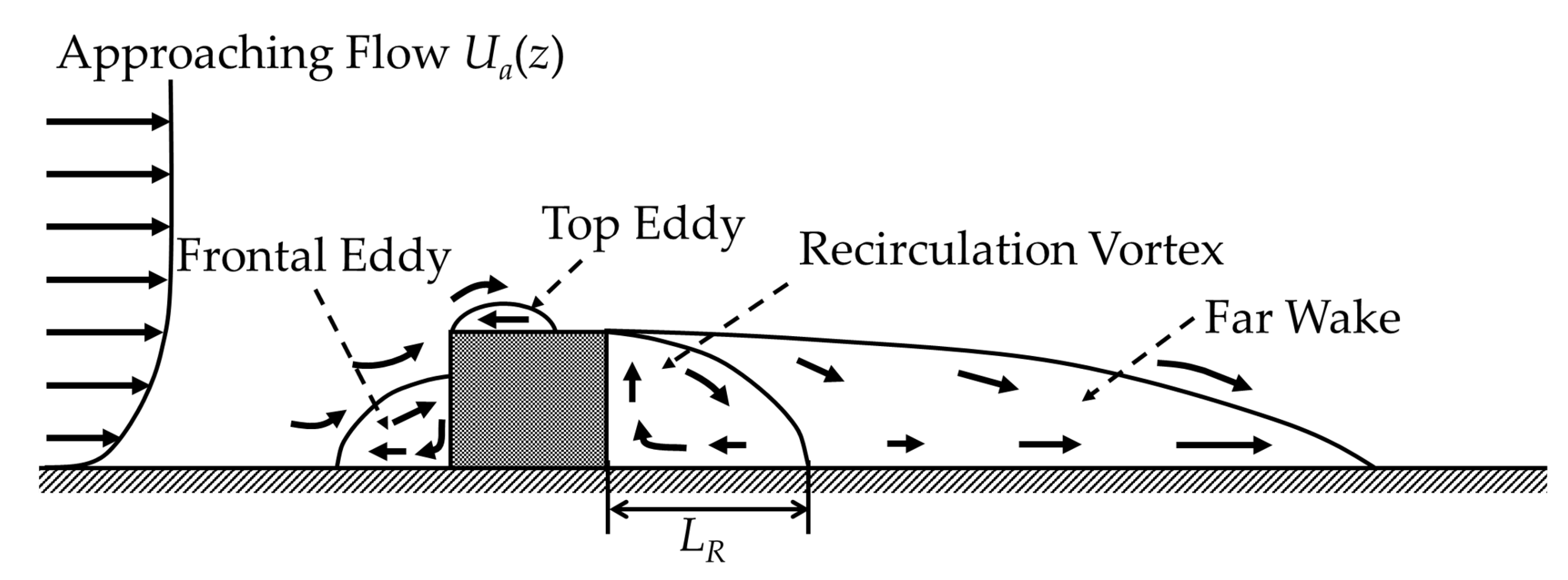
Figure 1 presents the typical flow pattern around a wall-mounted cube. In the QUIC model, the reattachment length from behind the cube is determined by the following equation that is derived by Fackrell and Pearce [12]:
where L, W and H denote the length, width, and height of the cube, respectively. The near-wake region of the leeward cube is defined by an ellipsoid shape, as in the following region:
where x represents the distance from the obstacle in the streamwise direction. The initial velocity component of x-direction is given by the following equation:
where the reference velocity was set to the inflow velocity at the height of the windward cube. is the distance from the back of the cube to the arbitrary x position in the near-wake region, while is the distance between the boundary of the near-wake region and behind the cube.
Oka (2014) [13], one of the co-authors of this paper, reported Röckle’s model and its revisions implemented in the QUIC, which were applied to the flow around the surface-mounted cube in the channel of the parallel flat plates. The obtained results agreed well with the experiment conducted by Hussein and Martinuzzi (1996) [14]. Accordingly, Oka concluded that the algebraic approach with the MASCON model is a significantly cost-efficient computational method, and it is suitable for the fast simulation of the steady state of the flow field.
In contrast to the wall-mounted cube, a different flow pattern appears in the near wake region of a vehicle. Figure 2 presents the schematic diagram of the flow pattern of a vehicle. Two streams, one flowing over the ceiling (upper stream) and the other under the vehicle (lower stream), are instantaneously detached from the back of the vehicle and merged at a slightly downstream location. At the inner region of the merged streams, two recirculation vortices, rotating in opposite directions to each other, are formed.
Conventional models can only apply a single recirculation vortex. Therefore, no model can reproduce the two recirculation vortices that are generated by the two upper and downstream streams behind the vehicle. In this study, we have developed an algebraic model of the two recirculation vortices that are applicable to the near-wake region based on the revised Röckle model. When considering the elliptical shape of the near-wake region behind the vehicle in the x-z section and the two recirculation vortices formed in the upper and lower halves of the ellipse, Equation (8) is modified for the near-wake region, as follows:
where and represent the floor height and distance between the ground and top of the vehicle’s rear, respectively. Similarly, for the geometric dimension H shown in Equation (7), which determines the length of the near-wake region, considering the shape of the rear of the vehicle generating the recirculation vortices, is modified in the following equation:
The initial velocity component was obtained in accordance with Equation (9), similar to the conventional Röckle model. In addition, we tentatively implemented the far-wake model of the QUIC model that was reported by Singh et al. (2006) [15], which is a modified version of Röckle’s model. Because the virtual origin of the velocity deficit equation was not explicitly defined in the paper by Carpentieri et al. (2012) [7], the correct results have not been obtained in our trial implementation. In the QUIC model, the far-wake region is defined at the back end of the near-wake region and within the region that is given by the following equation:
Regarding the initial estimate of the velocity, denotes the distance between the boundary of the far-wake region and the back of the cube, and it is similar to the near-wake model, and it is defined, as follows:
2.3. Computational Fluid Dynamics Model (CFD)
In this study, the OpenFOAM is adopted as the CFD model. OpenFOAM, which is the CFD toolbox written in C++ language (available at https://github.com/OpenFOAM accessed on 21 November 2020), is one of the most popular open-source codes in the world. The OpenFOAM model is parallelized by an efficient distributed-memory parallel programming via message passing interface (MPI). The OpenFOAM version 7.0 (The OpenFOAM Foundation, London, UK), which is the stable and previous version, is adopted for the incompressible steady flow simulation.
3. Test Case and Computational Conditions
3.1. Test Cases of Wind Tunnel Tests with 25% Scaled Model of the DrivAer Model
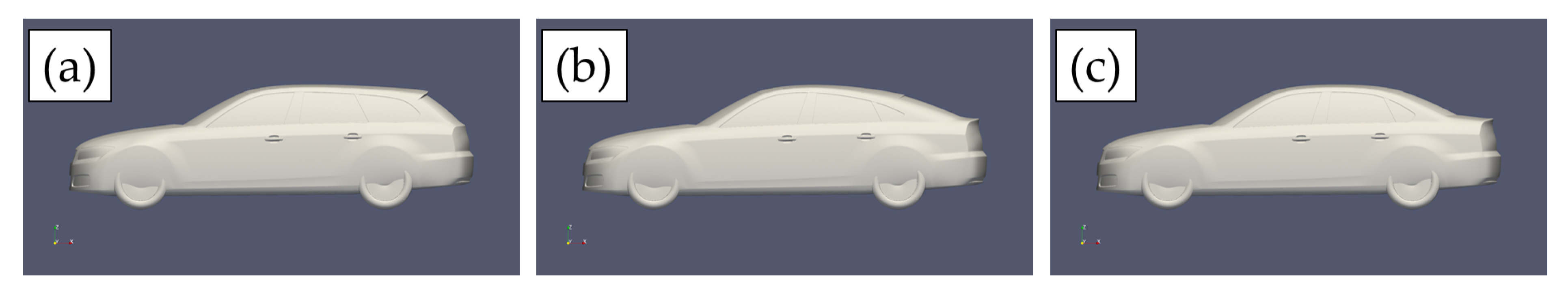
The DrivAer model is a generic vehicle model developed by the Institute of Aerodynamics and Fluid Mechanics at the Technische Universität München [16] for the aerodynamic investigations of passenger vehicles, as shown in Figure 3. The dimensions of the full-scale model of the DrivAer model are 4613 mm in length, 1820 mm in width, and 1418 mm in height. In this study, wind tunnel tests with a 25% scaled model of the DrivAer model, which were conducted by the Loughborough University and reported by Varney et al. [8], are adopted as the test cases for the numerical simulation. Hence, the dimensions of the scaled vehicle model are 1153.25 mm in length, 455 mm in width, and 354.5 mm in height. The wind tunnel facility consists of a test section with dimensions of 3600 mm × 1920 mm × 1320 mm (length × width × height). The representative velocity is set to 40 m/s. Here, the kinematic viscosity of air is m/s, and the total length of the vehicle is assumed to be a representative length, whereas the Reynolds number () is calculated as . Our algebraic model is applicable when the hypothesis of the Reynolds number independence is satisfied. The Reynolds number independence appears between 11,000 and 99,000 in the case of the surface-mounted cube described in the EPA Guideline [17]. In the blunt-shaped Bus case, Solmaz et al. [18] investigated the Reynolds number independence on the drag coefficient experimentally and via CFD, and they reported that it appeared approximately more than 55,000. Strangfeld et al. [19] reported that the results of a wind tunnel experiment with the 25% scaled fastback model of the DrivAer model indicated a Reynolds number independence in the range of . Because our algebraic model intends to reproduce the flow pattern and not for the aerodynamic study, the applicable range of in this study may be wider than that of the aerodynamics case. However, we expect that is the minimum value of the applicable range of Reynolds number.
3.2. Computational Conditions
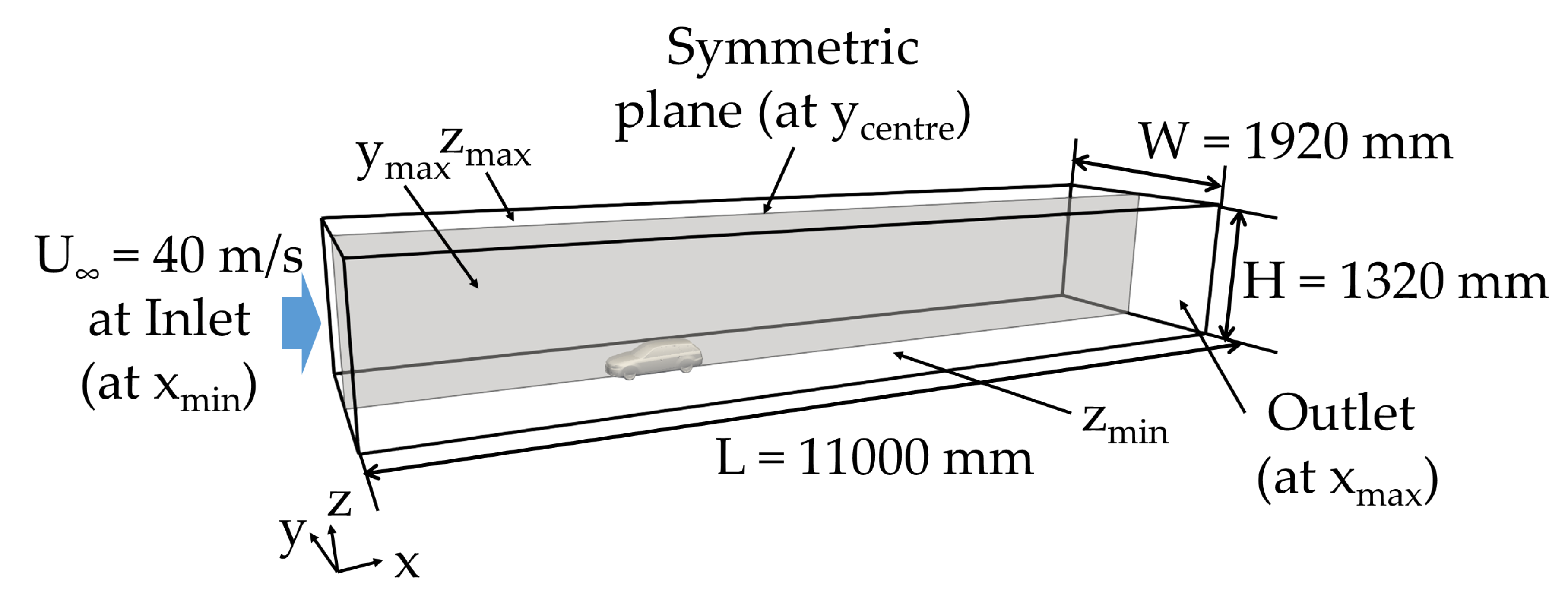
Computational domains are set similar to that of the wind tunnel experiment’s test section, except for its length, in order to obtain sufficient numerical data in the wake region, as shown in Figure 4. The validation cases of the DrivAer model provided by Wolf Dynamics (available at http://www.wolfdynamics.com/tutorials.html?id=152 accessed on 21 November 2020) are adopted as a basis, and they are modified to be suitable for our calculation. A number of cells are set to approximately cells for the half model with a cut through the symmetry plane and center of the y-direction in the CFD simulation, which is 960 mm in width as a half of the wind tunnel.
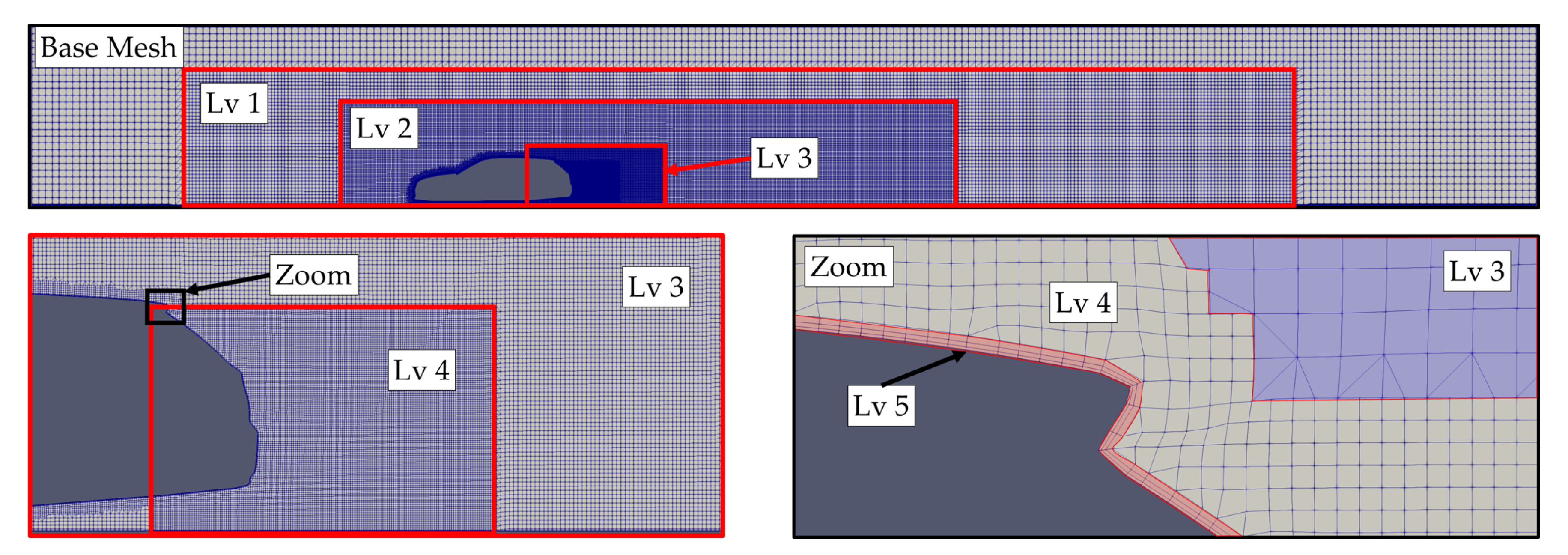
In the CFD simulation, the base mesh that consists of 0.2 m of regular grids is generated using blockMesh application and refined to five levels of fineness using the snappyHexMesh application. Figure 5 shows the schematic diagram of the mesh configuration. The finest mesh, denoted as Lv 5 in Figure 5, is set along the surface of a car body and the ground. The layer thicknesses of 0.0004, 0.0006, and 0.001 m from the surface of a car body are placed. The meshes lower level than Lv 5 are step-wisely set as 0.0125 mm in Lv 4, 0.025 mm in Lv 3, 0.05 mm in Lv 2, and 0.1 mm in Lv 1, respectively. The Lv 4 fineness mesh is additionally given at the near-wake region to ensure the adequate mesh resolution.
In contrast, the computational domains of the full model of the wind tunnel are set for the MASCON model, and three resolutions of mesh sizes, including 1,738,880 cells ( = 440, = 76 and = 52), 5,868,720 cells ( = 660, = 114 and = 78), and 13,911,040 cells ( = 880, = 152 and = 104), are tested to determine the suitable conditions for the simulation. The mesh of the MASCON model is based on the simple regular grids.
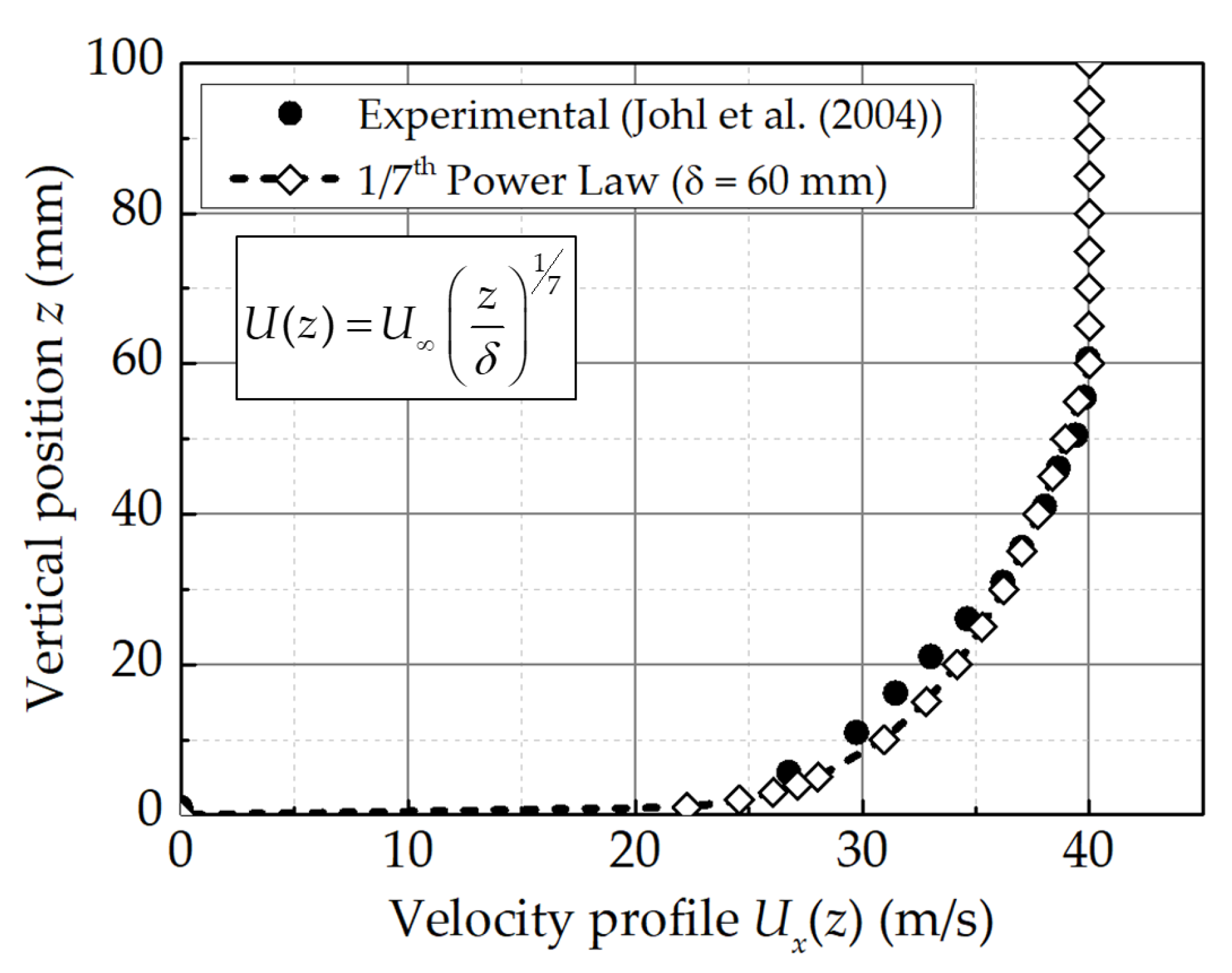
The experimental data of inflow velocity were reported by [20]. Subsequently, to assume the boundary condition of inlet velocity, we adopt the Blasius boundary layer profile following a th power-law with a boundary layer thickness () of 60 mm, as illustrated in Figure 6. Table 1 and Table 2 summarise the boundary conditions in the CFD simulation.
In the CFD simulation, the pressure-velocity coupling is performed by using the SIMPLE algorithm implemented in simpleFoam. The k-omega SST turbulence model [21] is adopted for the Reynolds Averaged Navier Stokes (RANS) simulations. The average, minimum and maximum values of the are 20.917, 1.0346 and 266.46 in the estateback model, respectively. Although the k-Omega SST turbulence model should be used with , the near-wall treatment developed by Menter et al. [22] enables the computed wall shear-stress varies by less than 2%, and all of the solutions follow the logarithmic profile in the wide range of the values from 0.2 to 100. Accordingly, we consider that the mesh configuration of the CFD simulations generally satisfies the above recommendation for practical applications. Table 3 summarises the solver settings of the CFD simulation. The pressure equation is solved by the GAMG solver with the Gauss–Seidel smoother and the tolerance and relative tolerance are set to and 0.01, respectively. On the other hand, the PBiCGStab solver with the DILU preconditioner is utilised to solve the rest equations, such as U and turbulence equations. The tolerance and relative tolerance are set to and 0.001, respectively. In addition, because we assume a vehicle is in parking condition, the motion of wheels are changed to the stationary state from the original rotational configuration of the Wolf dynamics.
4. Results and Discussion
In this section, we present the results and comparisons of the simulations that were obtained from two models and experiments, and we then discuss their practicality in terms of reproducibility and computational cost.
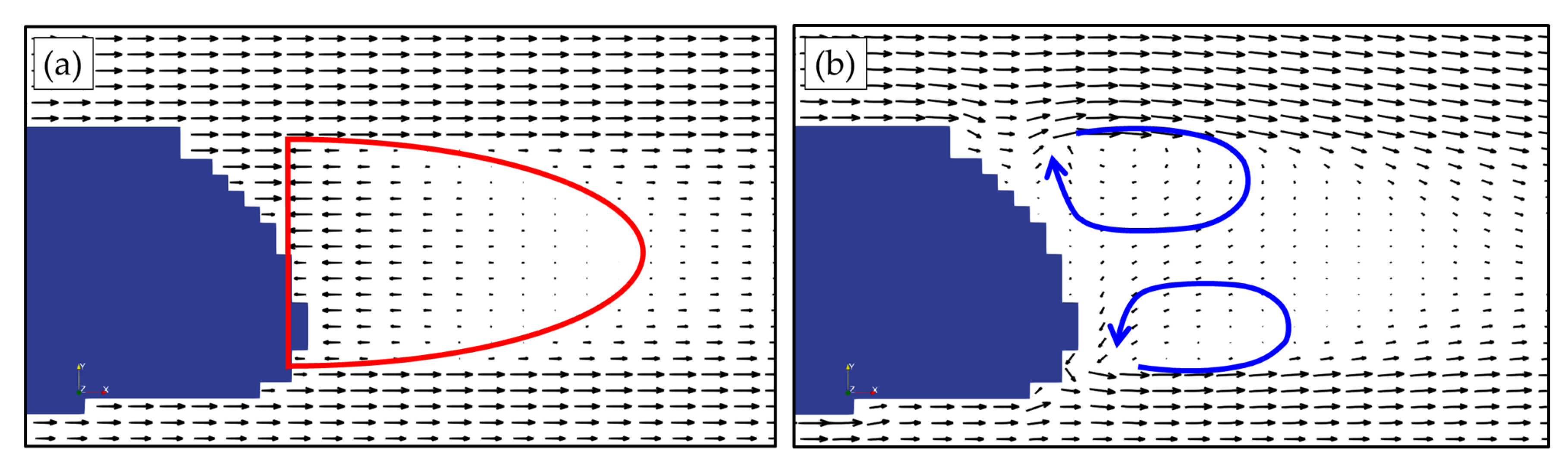
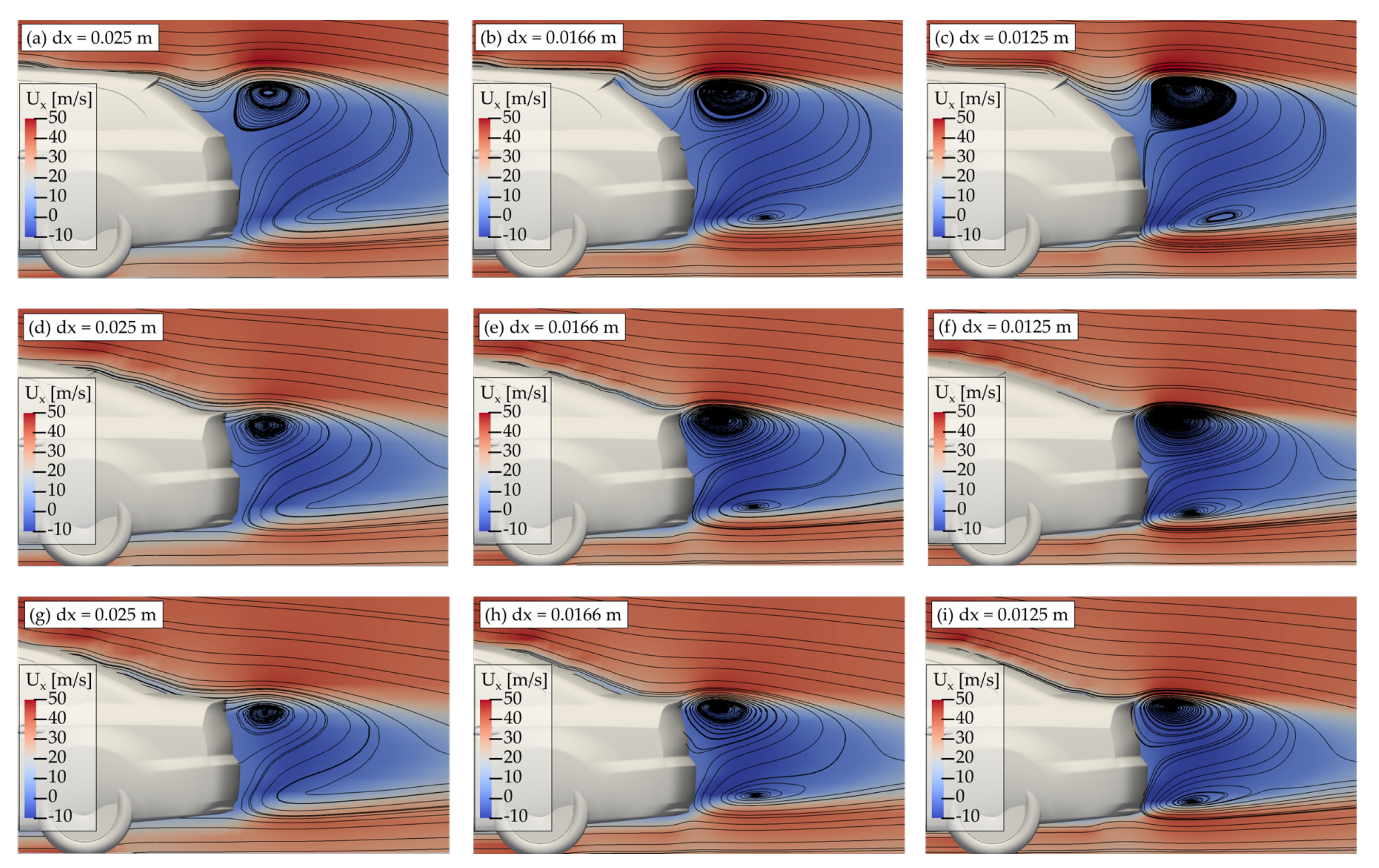
First, we investigate the optimal mesh resolution of our proposed method on the reproducibility of recirculation vortices. Figure 7 shows the comparison between the initial and corrected velocity fields of the proposed model. In the figure on the left (Figure 7), the initial velocity vector is given in the opposite direction to the mainstream around the recirculation region. After the correction by the MASCON model, as shown in the right figure, it can be observed that the velocity vectors in the recirculation region are varied in a swirling manner. Figure 8 presents the results of the simulations that were obtained from the proposed method, with varying mesh sizes. Streamlines of recirculation vortices are clearly illustrated in the near-wake region along with the increment of the mesh resolutions. In the case of m, the recirculation vortices are unclear. Therefore, we determine that the minimum resolutions of the mesh size has been 0.0166 m, while considering the numerical costs, as described in Table 4.
In the CFD calculation, iterations of the pressure and velocity equations have not converged in all cases (described later in Computational costs). Simmonds et al. (2017) [23] pointed out that the RANS analysis for the DrivAer model using k-omega SST turbulence model experienced fluctuations due to a pseudo-unsteadiness in the flow. We consider that the pseudo-unsteadiness appears in our simulations. However, to avoid choosing the result of an arbitrary step, we reasonably calculate the numerical solutions by averaging over the additional 1000 steps from the end of the simulation in the same way as past study conducted by Heft et al. (2012) [16].
4.1. Estateback Model
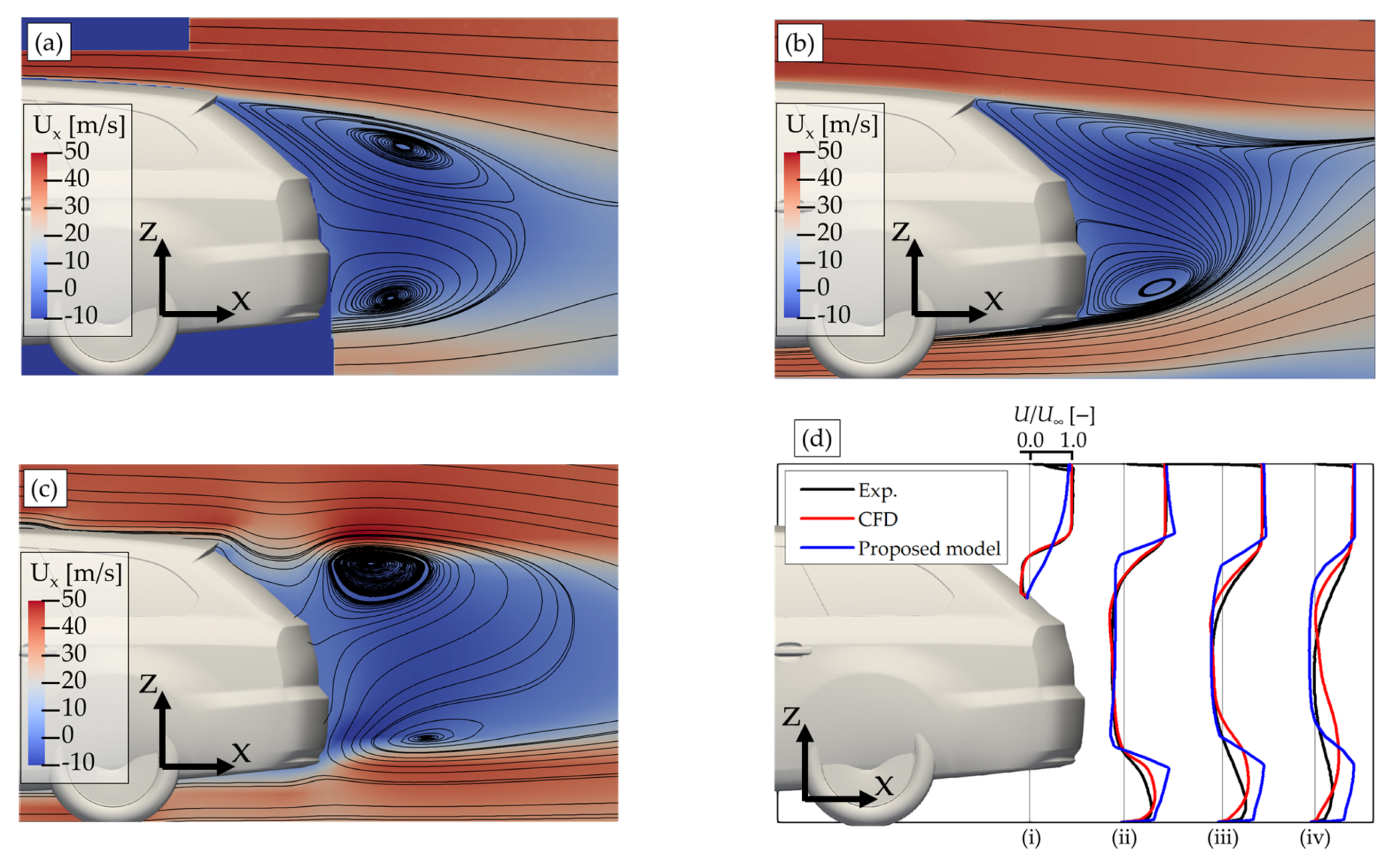
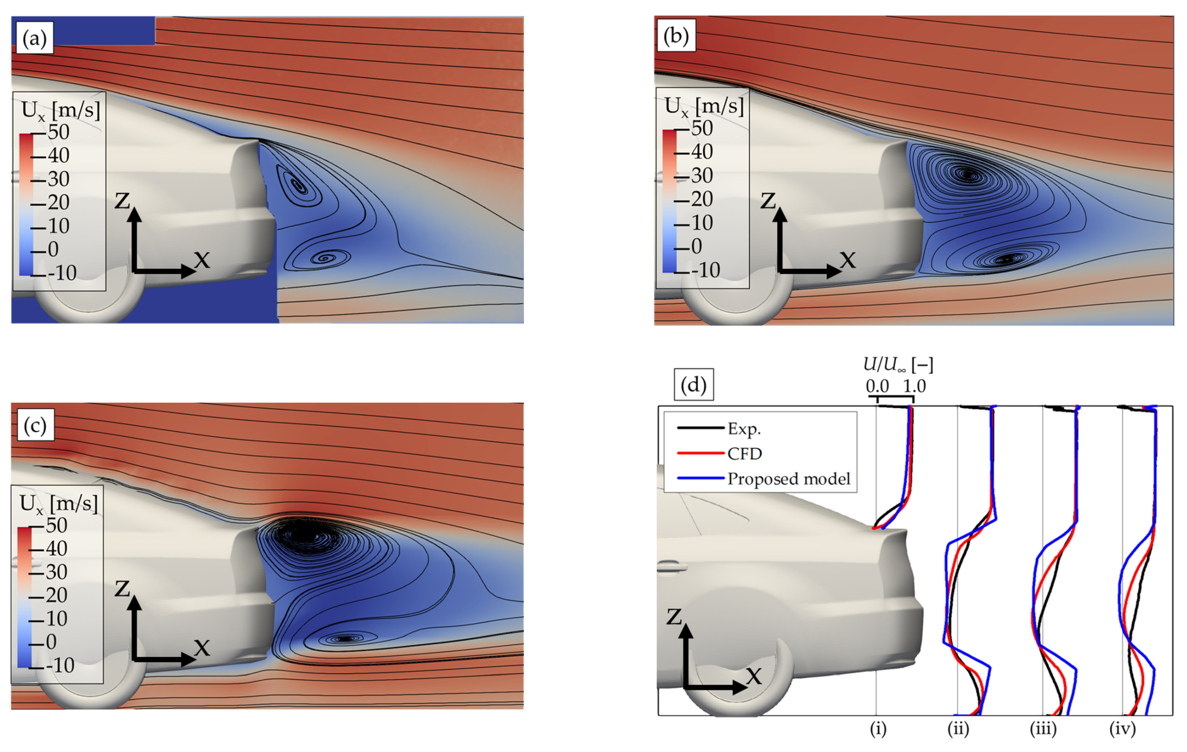
Figure 9 presents the comparisons of the streamlines and velocity profiles in the near-wake region between the experiment and two models. It can be observed that there are two recirculation vortices in the near-wake region for the experimental data. In the CFD result, the lower vortex appears successfully, whereas the upper vortex is unclear. On the other hand, although our proposed method successfully reproduces the two recirculation vortices, the streamline trajectories are slightly different from the experiments. To elucidate this result, we compare the vertical profile of the velocity at the four positions of the x-direction. The magnitude of the velocity deficit, which is expressed as the difference between the velocity profile of the approaching flow and actual velocity, is reproduced well by both CFD and the proposed method, but the shape of the distribution is not optimally reproduced. Therefore, it is inferred that the proposed method can generally reproduce the velocity profile of the experiment in the near-wake region.
4.2. Fastback Model
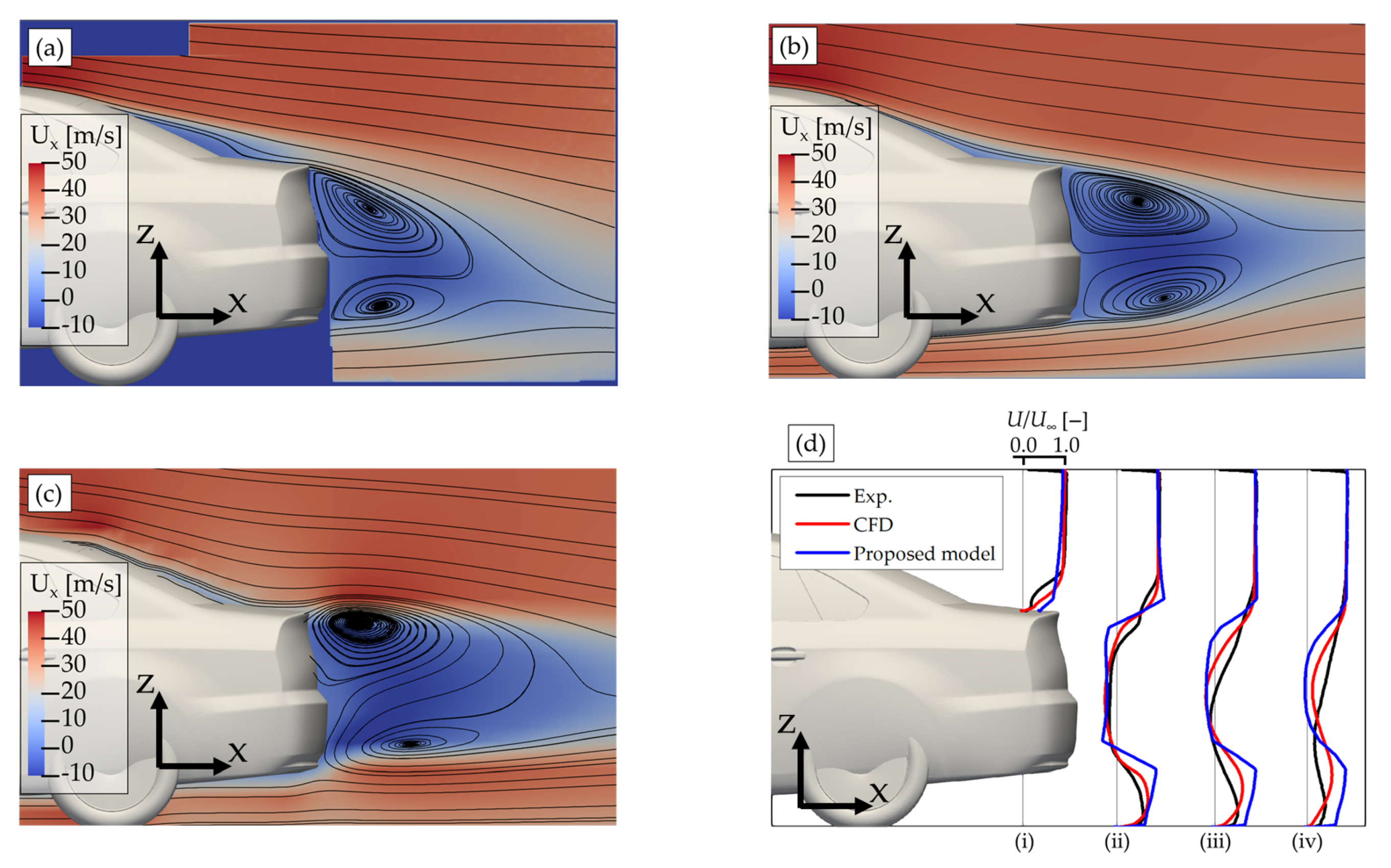
Figure 10 presents comparisons of the streamlines and velocity profiles in the near-wake region between the experiment and two numerical models in the case of the fastback model. In the results that were obtained from the experiment, two recirculation vortices also appear in the near-wake region. In contrast, two numerical models successfully reproduce two recirculation vortices that are similar to the experiment. However, the length of the near-wake region is over-estimated in the downwind direction of the two models. Although the trajectory of the near-wake region, which is the blue colored region presented in Figure 10a–c, extends towards the ground in the experiment, the near-wake region shows a horizontal extension in the two numerical models. These differences are also observed in the vertical profile of the local velocity, as illustrated in Figure 10d. These differences may be induced, owing to the alterations in the direction of the near-wake flow by the shape of the vehicle’s rear. The proposed algebraic model solely considers the vehicle’s geometric dimensions and it does not consider the effect of the vehicle’s actual rear shape. Hence, we conclude that the proposed algebraic model requires further improvement in the inclusion of the effects of the vehicle’s rear shape.
4.3. Notchback Model
Figure 11 presents the comparisons of the streamlines and velocity profiles in the near-wake region between the experiment and two numerical models. In the experimental result, two recirculation vortices are formed in a similar manner to the previously discussed two vehicle models. Regarding the result of the CFD model, although the trend in the lower recirculation vortex is slightly different from that of the experiment, the simulation generally reproduces the experiment. On the other hand, the formation of two recirculation vortices in the near-wake region is also observed in the results that were obtained from the proposed model. In addition, in the near-wake region, the differences in velocity deficit in the vertical velocity profiles appear to be similar to those discussed for the fastback model. Therefore, we infer that modifications to our algebraic model, as concluded in the Fastback model subsection, will also improve the reproducibility of the flow of recirculation vortices in the near-wake region for the Notchback model.
4.4. Practicality
Finally, we discuss the practicality of the two models in terms of the accuracy and computational costs.
4.4.1. Accuracy
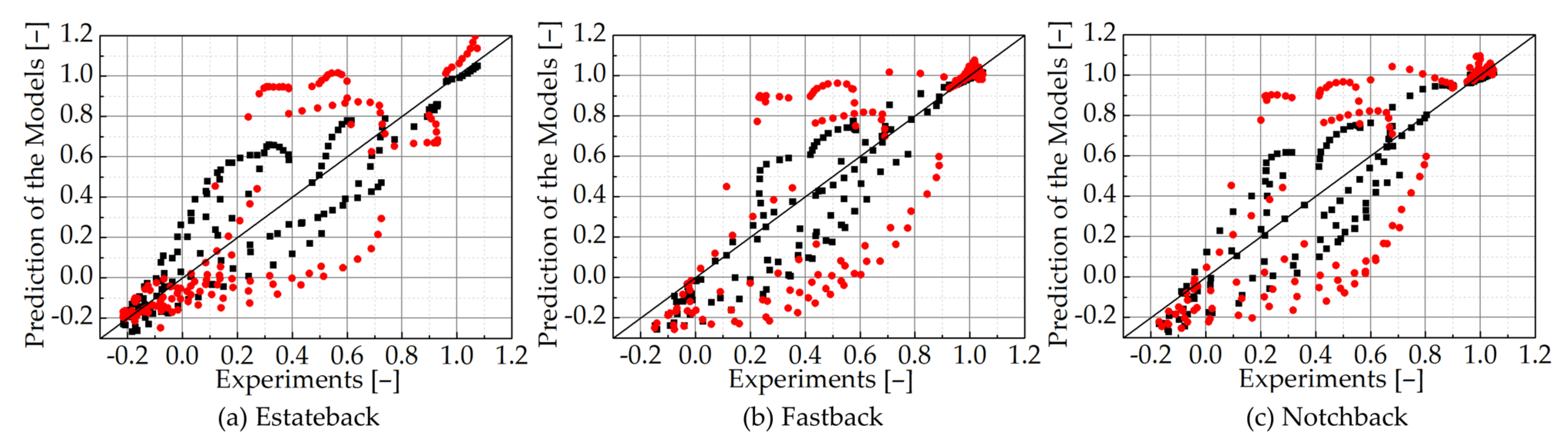
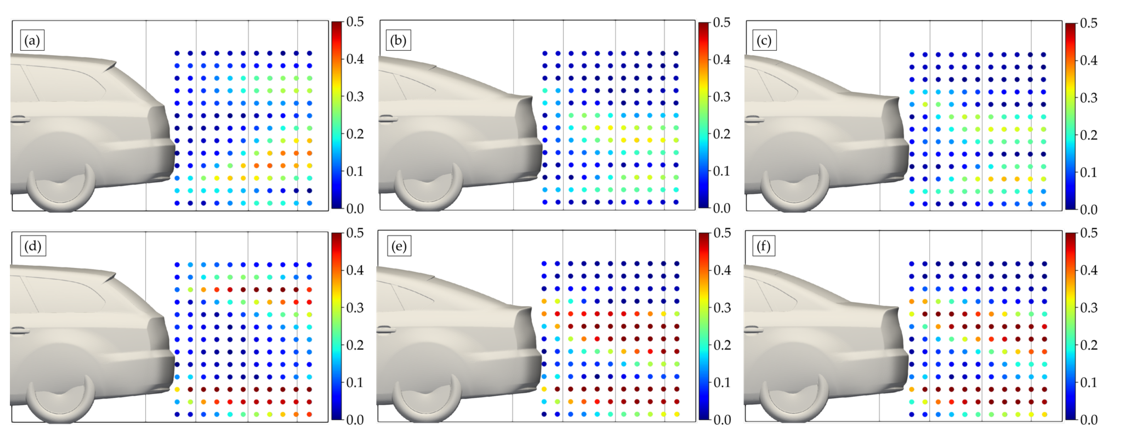
Regarding accuracy, 143 points of data are sampled in the near-wake region, 11 from 0.95985 m to 1.251 m in the x-direction, and 13 positions from 0.01591 m to 0.34586 m in the z-direction. Local velocity data that are normalised by the representative velocity, = 40 m/s, are compared between the experiment and the two models, as presented in Figure 12. If the plots are located closer to a diagonal line, it indicates that the model reproduces exactly in the experiment. It can be seen that the CFD model is better than the proposed method in terms of accuracy, with the overall plots being closed to diagonal lines in all three vehicle models. On the other hand, in the proposed model, the flow pattern of the estateback model can be reproduced better than the other two vehicle models. Figure 13 plots each sampled position colored in accordance with the difference in values between the experiment and the two numerical models. Because our algebraic model does not accurately consider the shape of the recirculation vortices, the error of the proposed method is particularly distributed at the boundary between the near-wake region and main flow, as indicated by the deeper red plots. To statistically and quantitatively evaluate these results, the root mean square error (RMSE) of the difference between the experimental data and the two numerical models is calculated and summarised in Table 5. For each of the vehicle models, the CFD model shows less error from the experimental values than from the proposed model. However, calculations using the proposed model verify that the estateback model indicates the least error and most reproducible results among the three models.
4.4.2. Computational Costs
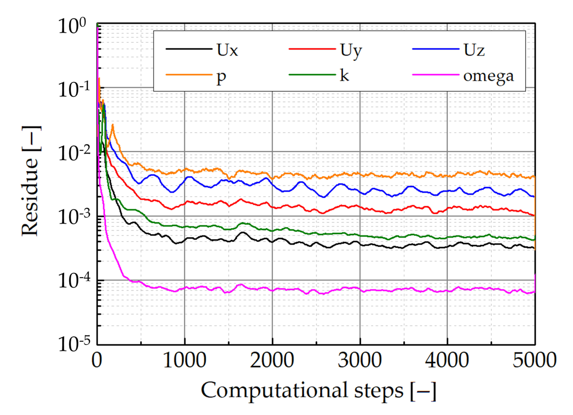
Regarding computational costs, Table 5 summarises the elapsed times for the computation. In the case of the CFD model, residues of velocity, pressure, turbulence energy, and omega in the iteration have not been reduced at approximately after 1000 steps, as illustrated in Figure 14, such that the CFD calculations have not reached the steady state, despite the elapses of 100,000. The CFD model has taken approximately 300 times longer than the proposed method to obtain the results at 5000 steps. Therefore, we have concluded that the proposed method can be more practical than the CFD model in terms of computational costs.
5. Conclusions
In this study, we have developed an algebraic model for reproducing the flow pattern in the near-wake region of a vehicle, and evaluated it by comparing with the experiment. We have verified its practicality in terms of accuracy when compared with the experiment using a 25% scaled wind tunnel. In addition, we have confirmed and compared the computational costs of the CFD and our algebraic model with the MASCON model. Consequently, the conclusions drawn from this study are summarised, as follows:
- In general, our algebraic model that was implemented in the MASCON model successfully reproduces two recirculation vortices in the near-wake region of the vehicle for the three vehicle shapes.
- The proposed method reproduces the flow pattern of the estateback model better than the other two vehicle models. However, the CFD model reproduces the flow pattern of the experiments better than our proposed method in the fastback and notchback models.
- In the CFD model, the residues are almost constant from approximately 1000 iterations, and they have never reduced below the criterion for determining the steady-state solution. Therefore, we have regarded the solution by averaging over the additional 1000 steps from the end of the simulation. If we assume that the time elapsed to reach 5000 steps is the computational times in the CFD model, then it takes approximately 300 times longer than the proposed method.
- The accuracy of reproducibility for the fastback and notchback while using the proposed method may be improved by revising the algebraic model to account for the rear shape of the vehicle.
- We conclude that the proposed method is practical in terms of the computational costs. Therefore, the algebraic model combined with the MASCON model would be a promising model that alternates the CFD model, by further improvement of the reproducibility.
Finally, we will continue to improve the accuracy of the algebraic model in the near-wake region. Accordingly, we will develop a model that can be applied to the far-wake region in order to more accurately reproduce the flow pattern around the vehicle.
Author Contributions
Conceptualization, data curation, methodology, validation, formal analysis, writing—original draft preparation and writing—review and editing, A.K., writing—review and editing, M.A., H.O. and Y.O.; supervision, H.O. and Y.O. All authors have read and agreed to the published version of the manuscript.
Funding
This work was supported by JSPS KAKENHI Grant Number JP19K04942.
Institutional Review Board Statement
Not applicable.
Informed Consent Statement
Not applicable.
Data Availability Statement
Data is contained within the article.
Conflicts of Interest
The authors declare no conflict of interest.
Abbreviations
The following abbreviations are used in this manuscript:
| OpenMP | Open Multi-Processing |
| API | Application Programming Interface |
| OpenFOAM | Open-source Field Operation And Manipulation |
| MPI | Message Passing Interface |
| CAD | Computer Aided Design |
| SIMPLE | Semi-Implicit Method for Pressure-Linked Equations |
| GAMG | Geometric agglomerated Algebraic Multi-Grid |
| PBiCGStab | Preconditioned Bi-Conjugate Gradient Stabilized |
| DILU | Diagonal Incomplete LU decomposition |
References
- Dickerson, M.H. MASCON—A Mass Consistent Atmospheric Flux Model for Regions with Complex Terrain. J. Appl. Meteor 1978, 17, 241–253. [Google Scholar] [CrossRef]
- Sherman, C.A. A Mass-Consistent Model for Wind Fields Over Complex Terrain. J. Appl. Meteor 1978, 17, 312–319. [Google Scholar] [CrossRef] [Green Version]
- Röckle, R. Bestimmung der Stomungsverhaltnisse im Bereich Komplexer Bebauugsstruckturen. Ph.D. Thesis, Vom Fachbereich Mechanik, der Technischen Hochschule Darmstadt, Darmstadt, Germany, 1990. [Google Scholar]
- VDI 3783 Blatt 10: Diagnostische Mikroskalige Windfeldmodelle—Gebäude und Hindernisumströmung. Available online: https://www.vdi.de/richtlinien/programme/inhalte-zu-richtlinien/vdi-3783-blatt-10-dmw (accessed on 21 November 2020).
- Los Alamos National Laboratory (LANL), The Quick Urban & Industrial Complex (QUIC) Dispersion Modeling System. Available online: https://www.lanl.gov/projects/quic/ (accessed on 21 November 2020).
- Eskridge, R.E.; Hunt, J.C.R. Highway modeling. Part I: Prediction of velocity and turbulence fields in the wake of vehicles. J. Appl. Meteor 1979, 18, 387–400. [Google Scholar] [CrossRef] [Green Version]
- Carpentieri, M.; Kumar, P.; Robins, A. Wind tunnel measurements for dispersion modelling of vehicle wakes. Atmos. Environ. 2012, 62, 9–25. [Google Scholar] [CrossRef] [Green Version]
- Varney, M.; Passmore, M.; Wittmeier, F.; Kuthada, T. DrivAer Experimental Aerodynamic Dataset. Loughborough University. Dataset. Available online: https://0-doi-org.brum.beds.ac.uk/10.17028/rd.lboro.12881213.v1 (accessed on 21 November 2020).
- Van der Vorst, H.A. Bi-CGSTAB: A Fast and Smoothly Converging Variant of Bi-CG for the Solution of Nonsymmetric Linear Systems. SIAM J. Sci. Stat. Comput. 1992, 13, 631–644. [Google Scholar] [CrossRef]
- Frankel, S.P. Convergence rates of iterative treatments of partial differential equations. Math. Tables Aids Comput. 1950, 4, 65–75. [Google Scholar] [CrossRef]
- Young, D.M. Iterative Methods for Solving Partial Differential Equations of Elliptic Type. Ph.D. Thesis, Harvard University, Cambridge, MA, USA, 1950. [Google Scholar]
- Fackrell, J.E.; Pearce, J.E. Parameters Affecting Dispersion in the Near Wake of Buildings; CEGB Report; RD/M/1179/N81; Marchwood Engineering Laboratories, Central Electricity Generating Board: London, UK, 1981; Available online: http://hdl.handle.net/10068/664612 (accessed on 21 November 2020).
- Oka, H. Application of a Diagnostic Urban Wind Model to Indoor Airflow Simulations—Model Evaluation against Flow around a Surface-Mounted Cube in a Plane Channel. J. JIME 2014, 49, 142–150. (In Japanese) [Google Scholar] [CrossRef]
- Hussein, H.J.; Martinuzzi, R.J. Energy Balance for Turbulent Flow around a Surface Mounted Cube Placed in a Channel. Phys. Fluids 1996, 8, 764–780. [Google Scholar] [CrossRef]
- Singh, B.; Pardyjak, E.R.; Brown, M.J. Testing of a Far-wake Parameterization for a Fast Response Urban Wind Model. In Proceedings of the 6th Symposium on the Urban Environment/14th Joint Conference on the Applications of Air Pollution Meteorology With the Air and Waste Management Association Atlanta, Atlanta, Georgia, 2 February 2006; Volume 11. [Google Scholar]
- Heft, A.; Indinger, T.; Adams, N. Investigation of unsteady flow structures in the wake of a realistic generic car model. In Proceedings of the 29th AIAA Applied Aerodynamics Conference, Honolulu, HI, USA, 27–30 June 2011. [Google Scholar]
- Snyder, W.H. Guideline for Fluid Modeling of Atmospheric Diffusion; U.S. EPA Report No.EPA-600/8-81-009; Environmental Sciences Research Laboratory, Office of Research and Development, US Environmental Protection Agency: Durham, NC, USA, 1981. [Google Scholar]
- Solmaz, H.; İçingür, Y. Drag Coefficient Determination of a Bus Model Using Reynolds Number Independence. Int. J. Automot. Eng. Technol. 2015, 4, 146–151. [Google Scholar] [CrossRef] [Green Version]
- Strangfeld, C.; Wieser, D.; Schmidt, H.J.; Woszidlo, R.; Nayeri, C.; Paschereit, C. Experimental Study of Baseline Flow Characteristics for the Realistic Car Model DrivAer; SAE Technical Paper; SAE International: Warrendale, PA, USA, 2013. [Google Scholar]
- Johl, G.; Passmore, M.; Render, P. Design methodology and performance of an indraft wind tunnel. Aeronaut. J. 2004, 108, 465–473. [Google Scholar] [CrossRef] [Green Version]
- Menter, F.R.; Kuntz, M.; Langtry, R. Ten Years of Industrial Experience with the SST Turbulence Model. Turbul. Heat Mass Transf. 2003, 4, 625–632. [Google Scholar]
- Menter, F.R.; Esch, T. Elements of Industrial Heat Transfer Prediction. In Proceedings of the 16th Brazilian Congress of Mechanical Engineering (COBEM), Uberlandia, Brazil, 26–30 November 2001.
- Simmonds, N.; Pitman, J.; Tsoutsanis, P.; Jenkins, J.; Gaylard, A.; Jansen, W. Complete Body Aerodynamic Study of three Vehicles. In Proceedings of the WCX17: SAE World Congress Experience, Detroit, MI, USA, 4–6 April 2017. [Google Scholar] [CrossRef] [Green Version]
Figure 1.
Schematic diagram of the flow patterns of a surface-mounted cube.

Figure 2.
Illustration of the flow pattern around a vehicle, along the centerline of the y-direction, in the x-z plane. Two recirculation vortices are formed in the near-wake region of a vehicle.
Figure 2.
Illustration of the flow pattern around a vehicle, along the centerline of the y-direction, in the x-z plane. Two recirculation vortices are formed in the near-wake region of a vehicle.

Figure 3.
Appearance of the DrivAer Models, as shown in (a) Estateback, (b) Fastback, and (c) Notchback. Only the rear shapes of the vehicles are different from each other.
Figure 3.
Appearance of the DrivAer Models, as shown in (a) Estateback, (b) Fastback, and (c) Notchback. Only the rear shapes of the vehicles are different from each other.

Figure 4.
Schematic diagram of the computational domains.

Figure 5.
Schematic diagram of the mesh configuration.

Figure 6.
Comparison of the inlet velocity profile of the experimental data with fitted curve using the Blasius boundary layer profile.
Figure 6.
Comparison of the inlet velocity profile of the experimental data with fitted curve using the Blasius boundary layer profile.

Figure 7.
Comparisons of the velocity fields between initial and corrected data in the case of m mesh resolution calculating the flow around the estateback model. The left figure (a) illustrates the initial and the right figure (b) represents the corrected data. The red line in the left figure denotes the recirculation region. The blue arrows illustrate the swirling regions.

Figure 8.
Comparisons of the streamlines calculated by the proposed method with varying mesh sizes. Upper three (a–c), middle three (d–f), and lower three (g–i) figures are the estateback, fastback, and notchback models, respectively. The Mesh sizes are = 0.025 m, 0.0166 m, and 0.0125 m, from the left to right figures.

Figure 9.
Streamlines and velocity profile in the near-wake region of the estateback vehicle, along the centerline of the y-direction, in the x-z plane. (a) Experiment [8], (b) CFD model, (c) Proposed model (d) comparisons of the velocity profiles. Velocity profiles are drawn from the front of the vehicle at downstream positions of (i) 1089 mm, (ii) 1199 mm, (iii) 1314 mm, and (iv) 1422 mm.

Figure 10.
Streamlines and velocity profile in the near-wake region of the fastback vehicle, along the centerline of the y-direction, in the x-z plane. (a) Experiment [8], (b) CFD model, (c) Proposed model (d) comparisons of the velocity profiles. Velocity profiles are drawn from the front of the vehicle at downstream positions of (i) 1089 mm, (ii) 1199 mm, (iii) 1314 mm, and (iv) 1422 mm.

Figure 11.
Streamlines and velocity profile in the near-wake region of the notchback vehicle, along the centerline of the y-direction, in the x-z plane. (a) Experiment [8], (b) CFD model, (c) Proposed model (d) comparisons of the velocity profiles. Velocity profiles are drawn from the front of the vehicle at downstream positions of (i) 1089 mm, (ii) 1199 mm, (iii) 1314 mm, and (iv) 1422 mm.

Figure 12.
Figures illustrating the variations in the models of the experimental data. Plots located close to the diagonal lines indicate better reproducibility of the experiments. The red and black colored plots denote the results of the proposed model and the CFD, respectively.
Figure 12.
Figures illustrating the variations in the models of the experimental data. Plots located close to the diagonal lines indicate better reproducibility of the experiments. The red and black colored plots denote the results of the proposed model and the CFD, respectively.

Figure 13.
Figure illustrating plots of each sampled positions colored in accordance with the difference in values between the experiment and two numerical models. Figure (a–c) illustrate the estateback, fastback, and notchback models obtained from the results of the CFD model. In addition, Figure (d–f) depict the estateback, fastback, and notchback models that were obtained from the proposed model.

Figure 14.
Figure showing the variations in the residues of each velocity component (,,), pressure (p), turbulence energy (k), and omega for the computational steps.
Figure 14.
Figure showing the variations in the residues of each velocity component (,,), pressure (p), turbulence energy (k), and omega for the computational steps.


Table 1.
Summary of the boundary conditions of the computational fluid dynamics (CFD) simulation. (U, p).
Table 1.
Summary of the boundary conditions of the computational fluid dynamics (CFD) simulation. (U, p).
| U | p | |
|---|---|---|
| Inlet () | type codedFixedValue; value uniform (0 0 0); redirectType velocityProfileInlet; | type zeroGradient; |
| Outlet () | type zeroGradient; value uniform (0 0 0 ); | type fixedValue; value uniform 0.0 |
| Symmetric plane () | type symmetry; | type symmetry; |
| type slip; | type slip; | |
| Ground () | type fixedValue; value uniform (0 0 0); | type zeroGradient; |
| type slip; | type slip; | |
| Vehicle body | type fixedValue; value uniform (0 0 0); | type zeroGradient; |
Table 2.
Summary of the boundary conditions of the CFD simulation. (k, omega, nut).
| k | Omega | Nut | |
|---|---|---|---|
| Inlet () | type fixedValue; | type fixedValue; | type zeroGradient; |
| Outlet () | type zeroGradient; | type zeroGradient; | type zeroGradient; |
| Symmetric plane () | type symmetry; | type symmetry; | type symmetry; |
| type slip; | type slip; | type slip; | |
| Ground () | type kqRWallFunction; | type omegaWallFunction; | type nutUSpaldingWallFunction; |
| type slip; | type slip; | type slip; | |
| Vehicle body | type kqRWallFunction; | type omegaWallFunction; | type nutUSpaldingWallFunction; |
Table 3.
Summary of the solver settings of the CFD simulation.
| Discretisation | Scheme | |
|---|---|---|
| ddtScheme | steadyState | |
| Gradient | cellLimited Gauss linear 1 | |
| Divergence | div(phi,U) | bounded Gauss linearUpwindV grad(U) |
| div(phi,k) | bounded Gauss upwind | |
| div(phi,omega) | bounded Gauss upwind | |
| div((nuEff*dev(grad(U).T()))) | Gauss linear | |
| Laplacian | Gauss linear limited 0.5 | |
Table 4.
Summary of the computational times required for the three vehicle models with three mesh resolutions. For all calculations, the BiCGStab method is adopted as the Poisson solver, and 16 threads are utilised for the parallel computations.
Table 4.
Summary of the computational times required for the three vehicle models with three mesh resolutions. For all calculations, the BiCGStab method is adopted as the Poisson solver, and 16 threads are utilised for the parallel computations.
| Vehicle Model | Computational Times | ||
|---|---|---|---|
| = 0.025 m | = 0.0166 m | = 0.0125 m | |
| Estateback | 7.49 s | 28.5 s | 75.5 s |
| Fastback | 8.53 s | 25.0 s | 64.5 s |
| Notchback | 9.24 s | 30.8 s | 76.3 s |
Table 5.
Summary of the computational environments, root mean square error of the results, and computational times.
Table 5.
Summary of the computational environments, root mean square error of the results, and computational times.
| Model | Computational | Vehicle | Root Mean | Computational |
|---|---|---|---|---|
| Environments | Type | Square Error | Times | |
| Intel Xeon Gold 6154 | Estateback | 0.178 | 9052 s | |
| CFD | 2 CPUs (36 Cores/72 Threads) | Fastback | 0.148 | 9543 s |
| Parallelized by MPI | Notchback | 0.155 | 9137 s | |
| Present | AMD Ryzen 9 4900HS | Estateback | 0.273 | 28.5 s |
| method | 1 CPU (8 Cores/16 Threads) | Fastback | 0.329 | 25.0 s |
| ( = 0.0166 m) | Parallelized by OpenMP | Notchback | 0.316 | 30.8 s |
Publisher’s Note: MDPI stays neutral with regard to jurisdictional claims in published maps and institutional affiliations. |
© 2021 by the authors. Licensee MDPI, Basel, Switzerland. This article is an open access article distributed under the terms and conditions of the Creative Commons Attribution (CC BY) license (http://creativecommons.org/licenses/by/4.0/).
Share and Cite
MDPI and ACS Style
Kimura, A.; Asami, M.; Oka, H.; Oka, Y. Development of an Algebraic Model of Empirical Parameterization of Near Wakes around a Vehicle. Fluids 2021, 6, 75. https://0-doi-org.brum.beds.ac.uk/10.3390/fluids6020075
AMA Style
Kimura A, Asami M, Oka H, Oka Y. Development of an Algebraic Model of Empirical Parameterization of Near Wakes around a Vehicle. Fluids. 2021; 6(2):75. https://0-doi-org.brum.beds.ac.uk/10.3390/fluids6020075
Chicago/Turabian StyleKimura, Arata, Mitsufumi Asami, Hideyuki Oka, and Yasushi Oka. 2021. "Development of an Algebraic Model of Empirical Parameterization of Near Wakes around a Vehicle" Fluids 6, no. 2: 75. https://0-doi-org.brum.beds.ac.uk/10.3390/fluids6020075