Article

Numerical Treatment of the Interface in Two Phase Flows Using a Compressible Framework in OpenFOAM: Demonstration on a High Velocity Droplet Impact Case

by
Giovanni Tretola
and
Konstantina Vogiatzaki
*
Advanced Engineering Centre, University of Brighton, Brighton BN2 4AT, UK
*
Author to whom correspondence should be addressed.
Submission received: 11 December 2020 / Revised: 27 January 2021 / Accepted: 28 January 2021 / Published: 9 February 2021
(This article belongs to the Special Issue Modelling of Reactive and Non-reactive Multiphase Flows)

Abstract

:
The ability to accurately predict the dynamics of fast moving and deforming interfaces is of interest to a number of applications including ink printing, drug delivery and fuel injection. In the current work we present a new compressible framework within OpenFOAM which incorporates mitigation strategies for the well known issue of spurious currents. The framework incorporates the compressible algebraic Volume-of-Fluid (VoF) method with additional interfacial treatment techniques including volume fraction smoothing and sharpening (for the calculation of the interface geometries and surface tension force, respectively) as well as filtering of the capillary forces. The framework is tested against different benchmarks: A 2D stationary droplet, a high velocity impact droplet case (500 m/s impact velocity) against a dry substrate and, with the same impact conditions, against a liquid film. For the 2D static droplet case, our results are consistent with what is observed in the literature when these strategies are implemented within incompressible frameworks. For the high impact droplet cases we find that accounting for both compressibility and correct representation of the interface is very important in numerical simulations, since pressure waves develop and propagate within the droplet interacting with the interface. While the implemented strategies do not alter the dynamics of the impact and the droplet shape, they have a considerable effect on the lamella formation. Our numerical method, although currently implemented for droplet cases, can also be used for any fast moving interface with or without considering the impact on a surface.

1. Introduction

In recent decades, a large volume of scientific research has been directed towards multiphase flows dominated by the influence of surface tension, including bubbles, drops, fluid films, jets and sheets. While most of these studies have been performed for incompressible flows there is still a wide range of applications for which fluid compressibility is of importance as for example for the case of high velocity droplet impact. Such impact cases are relevant to many industrial applications including applications that involve rotor blades. The repetitive impacts of liquid droplets onto rotor blades, at power generation and aerospace industries result in blade erosion and equipment failure. Another interesting application is coating technologies, where high speed molten metal or ceramic droplets impact onto a substrate. Finally high impact droplets have an application to ink printing.
Various physical phenomena occur during the impact of a liquid droplet on a solid substrate, such as the spreading, fingering, air entrapment, coalescence, shedding, solidification, bouncing, and splashing. Several reviews are present in literature that classify these different phenomena [1,2,3]. Physically these phenomena are mostly controlled by the fluid properties, the surface properties and the impact velocity. The interplay of all these factors is still far from being fully understood especially in high speed impact cases due to compressibilty effects. As the droplet impacts onto the surface, compression waves are created and propagate within the droplet resulting in local density variations which in turn might rapture the interface and give rise to jets as described in [4,5].
Numerical simulations are fundamental to highlight the role of the different physics behind droplet impact since they can provide insight into processes that experimentation is hard. For example, in the case of high speed droplet impact (of the order of 100 m/s and above) the timescale of impact is in the order of 1 ns, which requires a shutter speed of at least 10 9 fps for a sufficient temporal resolution [6]. Several numerical approaches have been proposed in the literature over the years for the modelling of multiphase interfacial phenomena. Great effort has been dedicated to correctly account for the transport of the interface and the consideration of the capillary forces. The role of the capillary forces is important both in cases with low velocity impact where capillary forces dominate throughout the process as well as to high impact case where although in the initial stages of the impact inertia is dominant as the droplets spread and slow down, capillarity becomes significant [7,8,9].
To transport the interface, the Volume Of Fluids (VOF) approach has been widely used in literature. Here, the different phases are tracked through the volume fraction, which is then used to reconstruct the interface. To represent the capillary force in this context, the Continuum Surface Force method [10] is widely adopted, which represents the surface tension force as a volumetric force. Despite the fact that this coupling has been used in multiphase simulations for the past decades, it has been shown that the coupling among transport schemes of the indicator function, surface tension in the Navier–Stokes equations and the curvature calculation still needs improvements [11]. Poor estimation and coupling of these terms results in the generation of spurious currents around the interface. Abadie et al. [12] showed the presence of the spurious currents within both the VoF as well as the Level Set, highlighting how the structure of the flow can be significantly modified by their presence. In the incompressible framework, different strategies to mitigate this problem have been proposed. Hysing et al. [13] proposed, in a finite element framework and using a Level Set function, an implicit and semi-implicit representation of the surface tension force, which improved the stability and reduced the spurious currents compared to the explicit formulation. Then, Raessi et al. [14] proposed the same formulation in a finite volume context for a coupled Level Set-Volume of Fluid method. The main benefit of the implicit formulation is that it allows to increase the time step constrain due to the capillary, reducing the computational cost without destabilising the solution. Focusing on VoF methods, Cummins et al. [15] and Popinet [11] have shown that calculating the interface properties based on the height function increase the accuracy of the interface curvature. More specifically, using the height function technique Popinet [11] showed an exact numerical balance between surface tension forces and the pressure jump with the elimination of the spurious currents in the case of a static interface. Denner et al. [16] imposed an exact curvature on both cartesian and tetrahedral meshes. In this case, the advection step had no influence on the spurious currents. In cases of practical interest, it is not possible to impose the curvature and the advection step introduces errors in the volume fraction fields and thus in the curvature estimation.
Raeini et al. [17] demonstrated how by working on the definition of the curvature calculation, and by filtering the capillary forces at the boundary, the magnitude of the spurious currents at the interface is reduced, improving the interface tracking for applications relevant to porous media. Aboukhedr et al. [9] aside from sharpening, smoothing and filtering algorithms for the interface capturing, introduced an adaptive interface compression scheme in order to allow for a dynamic estimation of the compressive velocity only at the areas of interest.
Various methods have been suggested for compressible interfacial flows context as well. So et al. [18] proposed a sharpening interface strategy for compressible VoF based methods, applied to droplet and shock-wave interaction. This was obtained through an anti-diffusion equation to counteract the numerical diffusion from the VoF discretisation. This strategy does not require an explicit reconstruction for the interface, reducing the computational cost and complexity. Then, Deng et al. [19] started from the method of [18] to present a new reconstruction scheme to improve the accuracy of the interface in compressible interfacial multiphase flows. Denner et al. [20] proposed a pressure-based algorithm for compressible interfacial flows.The discretisation method proposed performed local changes to the discrete values of density and total enthalpy based on the assumption of thermodynamic equilibrium, without the requirement of a Riemann solver. In this work, the advantages of a pressure-based formulation was highlighted, as it facilitates the definition of consistent mixture rules at the interface, including the Rankine-Hugoniot relations, and applies naturally to flows in all Mach number regimes. Finally, Nykteri et al. [21], simulated the droplet fragmentation from high velocity impact, employing a multi-scale methodology, to capture explicitly smaller (sub-grid) structures obtained from the impingement.
The goal of our study is to present a newly developed compressible VoF framework incorporating mitigation strategies for the spurious currents previously developed for incompressible frameworks [9,17,22,23] and to use this framework in order to highlight the effect that the spurious currents have on a quickly moving and deforming interface. First, the role of the spurious currents is highlighted for the well known benchmark case of a stationary droplet. Then, the influence of the mitigation strategies is observed for the high speed impact scenario. As a relevant case, the set up presented by Marzbali et al. [6] is investigated. First, a droplet impacting at high speed on a dry substrate is investigated. Then, a droplet impacting at the same conditions on a liquid film covering the substrate is also analysed. While in the current paper the framework is implemented for high speed droplets it is general enough to be implemented in any case of multiphase problems where compressibility is important and spurious currents require special treatment.

2. Methodology

Governing Equations

Our suggested framework is designed for simulations of compressible and immiscible fluids. The inteface tracking of the two-phase flow is performed with the VoF method as basis using the Open Source code OpenFOAM [24]. The native solver compressibleInterFOAM was used as starting point and modifications were made to account for the interface treatment.
Being a one-fluid method, the continuity, energy and momentum equation for the mixture are solved:
ρ t + · ρ u = 0 ρ u t + · ρ u u = · p d I + τ + ρ f b ρ T t + · ρ u T = · k T
where p d = p ρ g · x is the peziometric pressure, f b the body force and the mixture stress tensor τ is defined as
τ = μ u + u T 2 3 · u I
To track the single phase, the transport equation for the volume fraction is solved
ρ 1 α t + · ρ 1 α u = 0
as only two phases are present, the volume fractions obey the algebraic relationship α 1 + α 2 = 1 . The volume fraction is transported by the mixture velocity u.
When dealing with bounded scalars such as α , it is fundamental to respect the boundedness of the variable. For the α transport equation, Equation (3), the convective term can be source of unboundedness. Among the different strategies to mitigate the issue of the boundness, in this study the Multidimensional Universal Limiter with Explicit Solution (MULES), proposed by Weller [25], is adopted. The MULES limiter consists of an explicit solver which is based on the Flux Corrected Transport in order to maintain the boundedness of the scalar. A detailed description of the algorithm is beyond the scope of this study, and more details about its implementation can be found in literature [26]. Despite being derived in an incompressible framework, the MULES scheme can be directly applied to the compressible case. To be suitable to this scheme, the volume fraction equation is rearranged and the contribution from the compressibility is accounted numerically as a source term. This allows to hold a similar numerical methodology for the transport of the volume fraction between the compressible and incompressible solvers. The methodology presented is pressure-based, which means that the pressure is solved, with the phase densities obtained algebraically through the equation of state. The mixture density is defined as
ρ = ρ 1 α + ρ 2 1 α
The transport properties of the mixture are calculated from the single phase properties through the volume fraction, for example the viscosity is defined by μ = μ 1 α + μ 2 1 α .
As the gravity force is included in the pressure gradient through p d , the only body force present is the surface tension force. The surface tension force is treated as a pressure gradient across the liquid–gas interface and is calculated per unit volume based on the Continuum Surface Force (CSF) model proposed by Brackbill et al. [10].
f b = σ κ n I
where the mean interface curvature κ is defined as
κ = · n I
and the normal to the interface n I is defined as
n I = α | α |

3. Numerical Framework for the Interface Treatment

The numerical treatment of the interface properties and of the capillary force is presented in this section.

3.1. Discretisation of the Interface Curvature

After the value of the volume fraction at the cell centres is updated, the interface geometrical properties such as the mean curvature and its normal are calculated. From these properties the surface tension force for the momentum equation is then derived. To improve the accuracy of the the interface normal vectors near the interface, the volume fraction is subject initially to a smoothing process.
The smoothing process occurs in two stage: first the smoothed interpolating α from cell centres to face centres and then back to the cell centres recursively [17]. The smoothed volume fraction is then subject to a second cycle of smoothing, repeated two times, which consists into a weighted average of the volume fraction at the face with the face area. The smoothed volume fraction is then employed to calculate the interface normal vector n I from Equation (7).
Once the interface normal vectors are computed, the interface curvature can be obtained from n I through (6). The mean curvature calculated is smoothed in the direction normal to the interface recursively for two iterations ( i = { 0 , 1 } ), following Raeini et al. [17], as:
κ s , i + 1 = 2 α 1 α κ + 1 2 α 1 α κ s * , κ s , 0 = κ
with
κ s * = κ s , i w c f f c w c f f c , w = α 1 α + 10 6
The coefficient 2 α 1 α diffuses κ away from the interface, with minimum effect of the values of κ on the interface region. This is important for the stability of the numerical method. Furthermore, the interface curvature at face centres ( k f ) is obtained using a weighted interpolation method, as suggested by Renardy and Renardy [27]:
κ f = κ s , 2 w w , w = α 1 α + 10 6

3.2. Volume Fraction Sharpening and Capillary Forces

The capillary forces are calculated at the face centres, following Equation (11), as
f c , f = f c · n f = σ κ n s δ s f · n f = σ κ f δ s , f
where n f is the cell face normal, κ f is the face value of the curvature, Equation (10). The interface delta function δ s , f is calculated from the sharpened version of the volume fraction α s h a r p , as δ s , f = f α p c , where f denotes the gradient normal to the face f. Using δ s , f allows to control the sharpness of the capillary force, i.e., the thickness of the region where this force intervene.
The sharpened volume fraction α s h a r p , following Raeini et al. [17], is obtained by curtailing and then normalising the volume fraction α as
α s h a r p = 1 1 C p c min max α , C p c 2 , 1 C p c 2 C p c 2
A value of C p c = 0 lead to the original CSF (Continuum Surface Force) formulation (i.e., using α instead of α s h a r p for the interface location), while as C p c 1 , α s h a r p becomes sharper, leading to a sharper implementation of the capillary forces. For static cases a value of C p c = 0.98 is suggested [17], while C p c = 0.5 is used for the dynamic cases.

3.3. Filtering of the Capillary Forces

The adoption of δ s , f allows to mitigate the non-physical velocities at the interface. When interaction with a boundary is present though, Raeini et al. [17] showed that this may not be enough, and non-physical currents close to complex (curved or edged) solid boundaries can still be present. This problem can be solved modifying those components of the capillary forces that result in currents parallel to fluid interfaces trough the following operator:
f c , f , f i l t e r e d = f c , f f c , f , f i l t | |
where f c , f is calculated through Equation (11), and f c , f , f i l t | | is a time dependent term defined at the face centres.
Starting from zero as initial condition, this term is updated as:
f c , f , f i l t | | = δ s , f δ s , f + ϵ f c , f , f i l t | | o l d + C c , f , f i l t | | p c p c · n s n s f · n f
where f c , f , f i l t | | o l d represents the value of f c , f , f i l t | | at the previous time step.
The term δ s , f δ s , f + ϵ restricts the correction term to the region where the capillary force is present. Equation (14) gradually dampens those components of f c p c that are parallel to the interface, so that they finally converge to zero. This filtering may introduce small errors in the calculation, however the effect of this was observed to be negligible in the absence of non-smooth solid boundaries. The term C c , f , f i l t | | is a coefficient determining how fast the non–physical velocities are filtered. A value of C c , f , f i l t | | = 0.1 is used in [17]

3.4. Filtering Capillary Fluxes

Due to the numerical errors in the calculation of the interface curvature, it is difficult to obtain a zero net capillary force constraint (i.e., f c · S s = 0 , where S s is the interface area vector) when modelling the movement of a closed interface. This issue is evident for configuration at low capillary numbers [9,12,17]. In this study, this strategy will still be investigated even if the applications are characterised by high R e and W e , as the local capillary force where the interface is interacting with the boundary, may still play an important role in the process. Therefore, filtering the non-physical fluxes generated due to the inconsistent calculation of capillary forces is necessary to maintain the zero-net capillary force constraint.
A simple thresholding scheme to filter the capillary fluxes ϕ c = | S f | f c , f f p c can be used [17] in order to enforce a zero net capillary force flux on closed interface. This filtering will explicitly set the capillary fluxes to zero when their magnitude is of the order of the numerical errors.
The filtered capillary flux is defined as
ϕ c , f i l t = ϕ c max min ϕ c , ϕ c , t h r , ϕ c , t h r
where ϕ c , t h r is a threshold value below which capillary fluxes are set to zero. The threshold value is chosen as
ϕ c , t h r = C ϕ c , t h r | f c , f | a v g | S f |
where | f c , f | a v g is the average value of capillary forces (Equation (11)) over all faces where f c , v 0 . The coefficient C ϕ c , t h r define the threshold of the capillary fluxes to be filtered. This threshold indicates that the fluxes that are whithin this range of numerical error are filtered. For example, a value of C ϕ c , t h r = 0.01 implies that the capillary fluxes are set to zero if their magnitude is less than 1 % of the average of the capillary forces. The aim of this filtering is to prevent the capillary forces to cause instabilities or to introduce large errors in the velocity fields.

4. Results

To observe the influence of the different numerical treatments presented in Section 3, we investigate two cases: a benchmark case of a static droplet and a case of a high impact velocity droplet. Each case under investigation will be subject to the different stages of the interface treatment. The cases are named differently according to the treatments adopted. The nomenclature adopted is summarised in Table 1.

4.1. Static 2D Droplet

The first test case that we consider is the two dimensional static droplet. A cylindrical interface of radius r 0 = 0.125 m is initialised in a continuous phase without gravity. The disk is initially placed at the centre ( 0.5 , 0.5 ) of a 2D unit square domain. The diameter is chosen as a quarter of the domain to avoid the influence of the boundaries. The two phases consist of water and air at p = 101.3 kPa and T = 298 K, with the densities of ρ 1 = 998 kg/m3 and ρ 2 = 1.25 kg/m3. The surface tension is 0.072 N/m2. While for this case compressibility is not important it is used to demonstrate that the suggested framework can have applicability in both regions (compressible and incompressible)
Figure 1 shows the maximum velocity in the domain over time. The interface treatment reduces considerably the maximum velocity observed. The smoothing on only α and on both α and κ give a similar result, with the maximum velocity decaying faster and at a lower value than the original case. When the sharpening of the interface is introduced as well, the maximum velocity keeps decreasing, with no difference observed when the filtering is introduced.
Figure 2 shows the distribution of the velocity magnitude over time for the cases with static mesh at different times. The black line represents the iso-line of α = 0.5 .
The spatial distribution of the currents observed change with the different strategies implemented. With no smoothing, the initial velocity peaks decrease and distribute on the sides of the droplet. Furthermore, the parasitic currents extends from the interface outwards. Introducing the smoothing, these regions reduce their extent, and the influence of the spurious currents on the rest of the field is reduced as well. Looking at the results for both Sha VF and Filt f c , the distribution around the interface changes significantly. Apart from the more significant reduction compared to the previous case, the currents reduce their presence on the diagonal direction, and are more pronounced on the x and y directions. Overall, the domain influenced by the currents has reduced significantly with the introduction of the sharpening and further mitigated with the filtering.

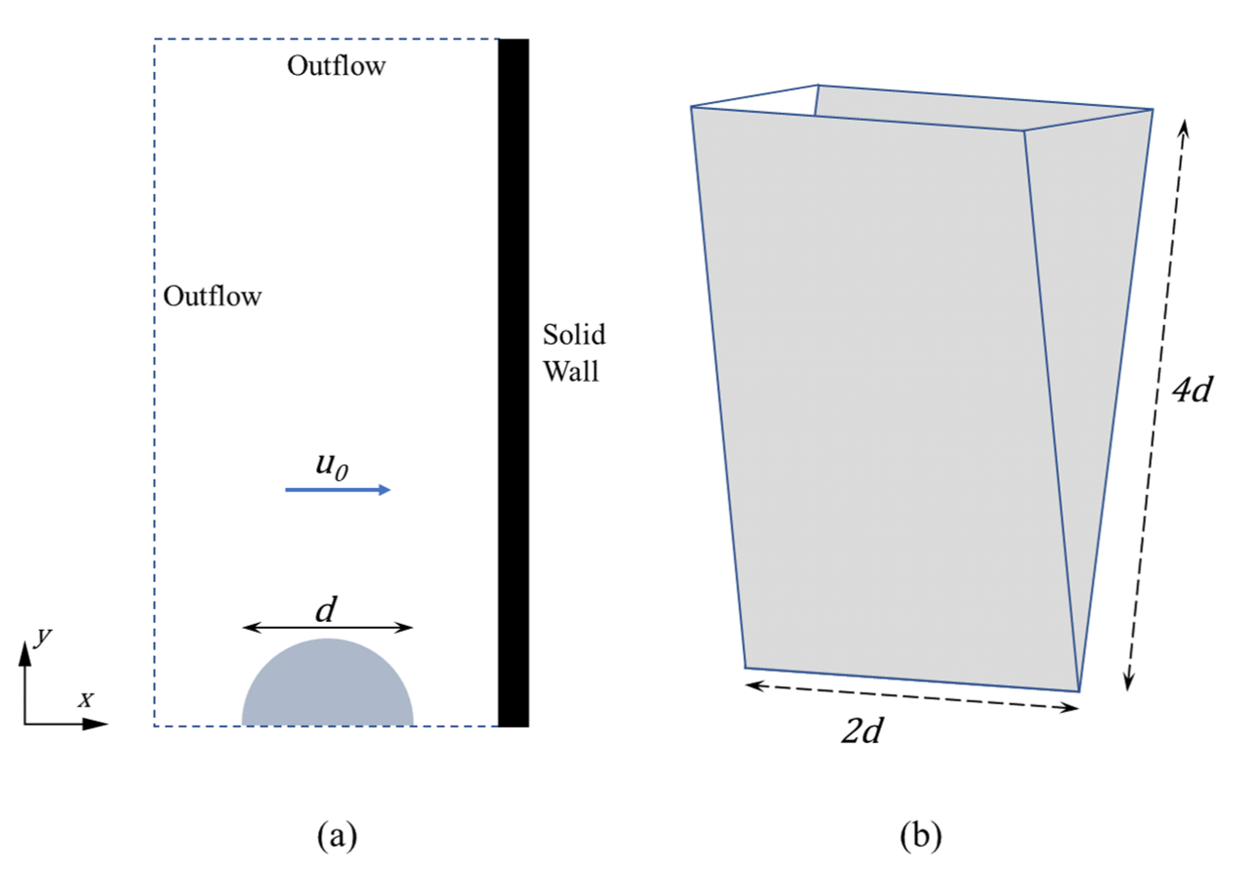
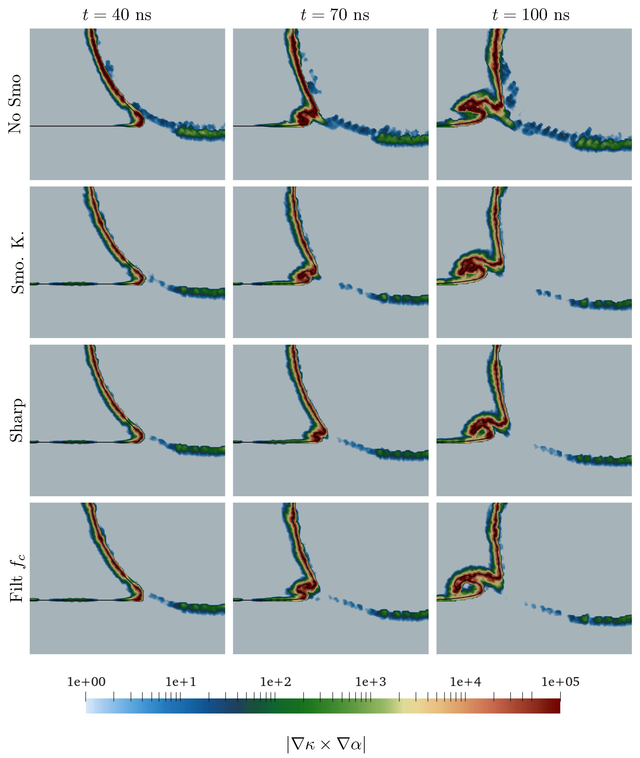
4.2. High Velocity Droplet Impact on a Dry Substrate

In order to assess the effect of the suggested numerical treatments on a moving interface, the set-up presented by Marzbali et al. [6] is simulated. A water droplet of radius r = 0.0001 m with impact velocity of u 0 = 500 m / s is investigated. The corresponding non-dimensional parameters are W e = 3.45 × 10 5 , R e = 6.024 × 10 4 and M a = 0.33 . These impact conditions are representative of a range of applications including the droplet impact with the rotor blade in the gas/steam turbines. In these configurations, the droplet flight speed is much lower than the blades velocity, which allows to assume the droplet stationary and the surface moving at the impingement velocity. This is equivalent to consider the droplet impacting at this velocity a stationary surface. Detailed experimental data of high-speed impact, in the order of 500 m/s, of single droplets are not available in literature. The complexity of the droplet impact at such conditions limits the experimental studies. Furthermore, it is worth noting that impacts at velocities over 100 m/s have timescales of the order of nanoseconds, which consists into a constraint about the temporal resolution of the equipment.
The computational domain for the 2D axisymmetric model, illustrated in Figure 3, has a width of 8 r , and the height of the domain is 4 r . The gravitational force is exerted in the same direction as the droplet impingement. The computational domain consists of air and water phases, with temperature and pressure of T = 300 K and p = 100 kPa for both phases. The outflow boundary condition is applied to all fluid boundaries except for the substrate surface, while no-slip, no-penetration, and adiabatic conditions are imposed on the fluid–solid interface as in Marzbali et al. [6]. Following Marzbali et al. [6], initially, the fluid domain is filled with air. At the beginning of each simulation, the droplet is patched in the fluid domain according to the impact conditions.
Regarding the equation of state, the ideal gas law is applied for the gaseous phase
ρ g = p R T
where R is the specific gas constant equal to 287 J/kg K for air. For the liquid phase, the power law equation of state proposed by Tait is employed:
ρ l = ρ l , 0 p + B p a + B 1 / A
where ρ l , 0 = 1000 kg/m3 is the density of the water at ambient condition, B = 300 MPa, p a = 0.1 MPa and A = 7.415 .
Figure 4 shows the contours of the velocity magnitude (left half of the droplet) and pressure gradient (right half of the droplet) at different instants for the different strategies.
After the impact, a high pressure region starts to built up close to the wall, as seen by the high region of | p | . This is caused by the compression of the liquid region. A propagation front of the pressure gradient is moving upstream within the droplet and it is reflected by the interface. This front acts also as a separator of the compressed and uncompressed region. As a result of the impact, and the increase of the local density at the impact point, lateral ejection of liquid is observed, characterised by velocity greater than u 0 . As the time progresses the compressed liquid region increases.
The propagation of pressure waves within the droplet and its interaction with the interface is important in high speed impact cases. After the impact, the waves travel upward. Reaching the upper part of the droplet, they are reflected downward interacting again with the wall [28].
The flow field distribution outside the droplet is shown in Figure 5, where the contours of Q criterion (left half) and vorticity magnitude (right half) are plotted for the different strategies at 70 ns.
The ejection of the lateral liquid at high velocity induces a propagation front into the stagnant field. The treatments of the interface overall reduces the vorticity at the periphery of the droplet.
As discussed in the research work of Abadie et al. [12], the generation of the spurious currents is related, in terms of vorticity, to the term κ × α . This term acts as a source term for vorticity when the capillary force is not balanced. For a detailed derivation of this term refer to Abadie et al. [12]. To better explain the influence of the interface treatment, the distribution of this term is piloted. Figure 6 shows the | κ × α | distribution at the region of the formation of the prompt jet from the droplet impact. The contours at different instants for the different interface treatment strategies are shown.
As expected, the intensity of the spurious currents is greater for the case with no treatment and they even expand at the internal part of the surface of the droplet. The different treatments reduce this intensity. Sharpening appears as more effective since the presence of the spurious currents is reduced at the interface while it is eliminated within the droplet.
To further clarify the role of the spurious currents and the difference among the different treatments for the lamella formation, Figure 7 which shows the velocity distribution around the lamella ejected at t = 100 ns, is also included. With no interface treatment (No Smo), more points of fragmentation are present. When sharpening of the volume fraction is implemented, this fragmentation starts later and the ejected jet is subject to lower values of | κ × α | . Looking at the direction of the velocity vectors at the lamella, it can be seen that with no treatment, the velocity vectors tend to lift while advancing towards the jet. This behaviour is altered by the smoothing and the sharpening of the volume fraction. By filtering the capillary forces, the lifting at the lamella is reduced and the velocity vectors become parallel to the wall.
This influence can be quantified looking at the spreading of the liquid at the wall, Figure 8. Reducing the spurious currents, the liquid ejected spreads slower, while no variation is observed with the introduction of the filtering.
Overall, the smoothing strategy does not influence significantly the dynamics of the impact at this velocity. Focusing on the morphology of the jet formed, differences are observed at the ejected liquid. At the droplet scale, the changes in the vorticity caused by the spurious currents do not change considerably the shape and the dynamics of the droplet. However, their effect is more pronounced on the lamella ejected which has thickness of few μ m and thus, is more sensitive to the artificial vorticity induced by the spurious currents. The spurious currents also alter the flow field close to the lateral jet: filtering the capillary forces allows to “straighten” the velocity field, as the vorticity induced by spurious currents on the lateral jet is mitigated.

4.3. Droplet Impact on Liquid Film

In the droplet impact framework investigations, another scenario of interest is the impact of the droplet on a liquid film that covers the dry substrate. This corresponds to the case where an array of droplets are injected in the domain. A previously impinged droplet has spread over the surface and the subsequent droplet impacts this liquid film rather than the dry surface. In this case presented here, a droplet with the same diameter and velocity as the previous case (Section 4.2) impacts on a liquid film of thickness h = d / 4 = 25 μ m . The initial configuration along with the computational domain is presented in Figure 9. The same domain, boundary conditions and the equation of state used in Section 4.2 are adopted.
Figure 10 shows the contours of the velocity magnitude (left side) and pressure gradient (right side) at different instants for the different strategies. After the impact, two high pressure fronts develop from the impact point at the liquid film: the first travel towards the droplet, the second towards the dry substrate. The latter is then reflected and two high pressure fronts travel across the droplet. Meanwhile, from the impact a liquid jet forms between the droplet and the film, ejecting with velocity double the impact one. This is consistent with the observation from literature [6].
To identify the behaviour of the spurious currents, the distribution of the term κ × α is observed as in the previous section. Figure 11 shows the | κ × α | distribution at the region of the formation of the prompt jet. Compared to the impact with a solid wall, when the droplet interacts with the liquid film the impact region between them is also subject to spurious currents. With no treatment, these currents surround the whole droplet and persist between the droplet and the film. With the introduction of interface treatments, these currents are mitigated especially between the droplet and the film.
Figure 12 zooms on the lamella ejection at t = 100 ns, where the velocity vectors are coloured by their magnitude and the black iso-line represents α = 0.5 . When the interface treatment is introduced, the ligament ejected points toward the film. Filtering the capillary forces shows a longer ligament than the previous treatments.

5. Conclusions

In this study, we present a compressible framework where a range of interfacial treatment techniques previously used within incompressible frameworks are implemented. We examine the effect these techniques have on fast moving interfaces. The interface treatment targets the reduction of the spurious currents. While for low velocity impact cases, these treatments have shown to significantly improve the numerical prediction, such investigation was not conducted for compressible frameworks before. After a first test on a static 2D case, a high velocity droplet impacting first on a dry substrate and then on a liquid film have been simulated to demonstrate the performance of the framework. Overall, the interface treatment did not alter the dynamics of the impact and the droplet shape, but had a interesting effect on the lamella. Despite the high velocities characterising the case, still the influence of the capillary force was observed on the lateral jet forming from the impact due to its small thickness. The interface treatment reduced the spurious vorticity on the ejected lamella, modifying its morphology. Also the flow field close to the lateral jet was affected, as once the filtering of the capillary flux is present, the velocity vectors become parallel to the wall. When the impact on a liquid film is considered, the interface treatment reduces the spurious currents not only around the interface but also between the droplet and the liquid film. Filtering the capillary forces reduces the vorticity around the ejected lamella, which is then more elongated. Further investigations are required, as the influence of the numerical treatment when adaptive mesh refinement at the interface is present.

Author Contributions

Conceptualisation, all authors; numerical methodology, all authors; simulations, G.T.; visualisation, G.T.; analysis, all authors; writing—original draft preparation, G.T.; writing—review and editing, K.V.; project administration, K.V.; funding acquisition, K.V.; supervision, K.V. All authors have read and agreed to the published version of the manuscript.

Funding

The funding for this project from the UK’s Engineering and Physical Science Research Council support through the grant EP/S001824/1 is gratefully acknowledged.

Institutional Review Board Statement

Not applicable.

Informed Consent Statement

Not applicable.

Conflicts of Interest

The authors declare no conflict of interest.

References

  1. Yarin, A. Drop Impact Dynamics: Splashing, Spreading, Receding, Bouncing…. Annu. Rev. Fluid Mech. 2006, 38, 159–192. [Google Scholar] [CrossRef]
  2. Marengo, M.; Antonini, C.; Roisman, I.V.; Tropea, C. Drop collisions with simple and complex surfaces. Curr. Opin. Colloid Interface Sci. 2011, 16, 292–302. [Google Scholar] [CrossRef]
  3. Josserand, C.; Thoroddsen, S. Drop Impact on a Solid Surface. Annu. Rev. Fluid Mech. 2016, 48, 365–391. [Google Scholar] [CrossRef] [Green Version]
  4. Heymann, F.J. High-Speed Impact between a Liquid Drop and a Solid Surface. J. Appl. Phys. 1969, 40, 5113–5122. [Google Scholar] [CrossRef]
  5. Dear, J.P.; Field, J.E. High-speed photography of surface geometry effects in liquid/solid impact. J. Appl. Phys. 1988, 63, 1015–1021. [Google Scholar] [CrossRef]
  6. Marzbali, M.; Dolatabadi, A. High-speed droplet impingement on dry and wetted substrates. Phys. Fluids 2020, 32, 112101. [Google Scholar] [CrossRef]
  7. Pasandideh-Fard, M.; Qiao, Y.M.; Chandra, S.; Mostaghimi, J. Capillary effects during droplet impact on a solid surface. Phys. Fluids 1996, 8, 650–659. [Google Scholar] [CrossRef]
  8. Yokoi, K.; Vadillo, D.; Hinch, J.; Hutchings, I. Numerical studies of the influence of the dynamic contact angle on a droplet impacting on a dry surface. Phys. Fluids 2009, 21, 072102. [Google Scholar] [CrossRef] [Green Version]
  9. Aboukhedr, M.; Georgoulas, A.; Marengo, M.; Gavaises, M.; Vogiatzaki, K. Simulation of micro-flow dynamics at low capillary numbers using adaptive interface compression. Comput. Fluids 2018, 165, 13–32. [Google Scholar] [CrossRef] [Green Version]
  10. Brackbill, J.U.; Kothe, D.B.; Zemach, C. A continuum method for modeling surface tension. J. Comput. Phys. 1992, 100, 335–354. [Google Scholar] [CrossRef]
  11. Popinet, S. An accurate adaptive solver for surface-tension-driven interfacial flows. J. Comput. Phys. 2009, 228, 5838–5866. [Google Scholar] [CrossRef] [Green Version]
  12. Abadie, T.; Aubin, J.; Legendre, D. On the combined effects of surface tension force calculation and interface advection on spurious currents within Volume of Fluid and Level Set frameworks. J. Comput. Phys. 2015, 297, 611–636. [Google Scholar] [CrossRef]
  13. Hysing, S. A new implicit surface tension implementation for interfacial flows. Int. J. Numer. Methods Fluids 2006, 51, 659–672. [Google Scholar] [CrossRef]
  14. Raessi, M.; Bussmann, M.; Mostaghimi, J. A semi-implicit finite volume implementation of the CSF method for treating surface tension in interfacial flows. Int. J. Numer. Methods Fluids 2009, 59, 1093–1110. [Google Scholar] [CrossRef]
  15. Cummins, S.J.; Francois, M.M.; Kothe, D.B. Estimating curvature from volume fractions. Comput. Struct. 2005, 83, 425–434. [Google Scholar] [CrossRef]
  16. Denner, F.; van Wachem, B.G.M. Fully-Coupled Balanced-Force VOF Framework for Arbitrary Meshes with Least-Squares Curvature Evaluation from Volume Fractions. Numer. Heat Transf. Part B Fundam. 2014, 65, 218–255. [Google Scholar] [CrossRef] [Green Version]
  17. Raeini, A.Q.; Blunt, M.J.; Bijeljic, B. Modelling two-phase flow in porous media at the pore scale using the volume-of-fluid method. J. Comput. Phys. 2012, 231, 5653–5668. [Google Scholar] [CrossRef]
  18. So, K.K.; Hu, X.Y.; Adams, N.A. Anti-diffusion interface sharpening technique for two-phase compressible flow simulations. J. Comput. Phys. 2012, 231, 4304–4323. [Google Scholar] [CrossRef]
  19. Deng, X.; Inaba, S.; Xie, B.; Shyue, K.M.; Xiao, F. High fidelity discontinuity-resolving reconstruction for compressible multiphase flows with moving interfaces. J. Comput. Phys. 2018, 371, 945–966. [Google Scholar] [CrossRef]
  20. Denner, F.; Xiao, C.N.; van Wachem, B.G. Pressure-based algorithm for compressible interfacial flows with acoustically-conservative interface discretisation. J. Comput. Phys. 2018, 367, 192–234. [Google Scholar] [CrossRef]
  21. Nykteri, G.; Koukouvinis, P.; Gonzalez Avila, S.R.; Ohl, C.D.; Gavaises, M. A Σ-Y two-fluid model with dynamic local topology detection: Application to high-speed droplet impact. J. Comput. Phys. 2020, 408, 109225. [Google Scholar] [CrossRef]
  22. Georgoulas, A.; Koukouvinis, P.; Gavaises, M.; Marengo, M. Numerical investigation of quasi-static bubble growth and detachment from submerged orifices in isothermal liquid pools: The effect of varying fluid properties and gravity levels. Int. J. Multiph. Flow 2015, 74, 59–78. [Google Scholar] [CrossRef] [Green Version]
  23. Bilger, C.; Aboukhedr, M.; Vogiatzaki, K.; Cant, R. Evaluation of two-phase flow solvers using Level Set and Volume of Fluid methods. J. Comput. Phys. 2017, 345, 665–686. [Google Scholar] [CrossRef] [Green Version]
  24. OpenCFD. OpenFOAM—The Open Source CFD Toolbox—User’s Guide; OpenCFD Ltd.: London, UK, 2018. [Google Scholar]
  25. Weller, H.G. A New Approach to VOF-Based Interface Capturing Methods for Incompressible and Compressible Flow; Report TR/HGW/04; OpenCFD Ltd.: London, UK, 2008. [Google Scholar]
  26. Damián, S.M. An Extended Mixture Model for the Simultaneous Treatment of Short and Long Scale Interfaces. Ph.D. Thesis, Universidad Nacional del Litoral, Santa Fe, Argentina, 2013. [Google Scholar]
  27. Renardy, Y.; Renardy, M. PROST: A parabolic reconstruction of surface tension for the volume-of-fluid method. J. Comput. Phys. 2002, 183, 400–421. [Google Scholar] [CrossRef] [Green Version]
  28. Haller Knezevic, K. High-Velocity Impact of a Liquid Droplet on a Rigid Surface the Effects of Liquid Compressibility. Ph.D. Thesis, ETH Zurich, Zurich, Switzerland, 2002. [Google Scholar]
Figure 1. Maximum velocity in the domain over time.
Fluids 06 00078 g001
Figure 2. Evolution of the velocity distribution for the different cases. Black line represents the iso-line of α = 0.5 . Different rows indicate the different solving strategy.
Fluids 06 00078 g002
Figure 3. Initial configuration and boundary conditions (a) with computational domain (b).
Fluids 06 00078 g003
Figure 4. Velocity and pressure gradient distribution within the droplet for the different smoothing strategies cases at different instants. Black line represents the iso-line of α = 0.5 .
Fluids 06 00078 g004
Figure 5. Q criterion and vorticity distribution at the droplet at 70 ns for the different smoothig strategies: (a) No. Smo.; (b) Sharp. V.F.; (c) Filtering f c . Black line represents the iso-line of α = 0.5 .
Fluids 06 00078 g005
Figure 6. Contour plot of | κ × α | at different instants, with the formation of the prompt jet from the droplet impact.
Fluids 06 00078 g006
Figure 7. Contour level of α = 0.5 , with velocity field arrows coloured by | κ × α | .
Fluids 06 00078 g007
Figure 8. Comparison between the different treatments of the liquid spreading at the wall. (a) Schematic of the liquid spreading y w . (b) Evolution over time of y w for the different treatments.
Fluids 06 00078 g008
Figure 9. Initial configuration and boundary conditions (a) with computational domain (b).
Fluids 06 00078 g009
Figure 10. Velocity and pressure gradient distribution within the droplet for the different smoothing strategies cases at different instants. Black line represents the iso-line of α = 0.5 .
Fluids 06 00078 g010
Figure 11. Contour plot of | κ × α | at different instants, with the formation of the prompt jet from the droplet impact.
Fluids 06 00078 g011
Figure 12. Iso-line α = 0.5 , with velocity field arrows coloured by | u | .
Fluids 06 00078 g012
Table 1. Names of different strategies.
StrategyNo Smo.Smo. V.F.Smo. KShar V.F.Filt f c
Smoothing of α
Smoothing of κ : Equations (8) and (9)
Sharpening of α : Equation (12)
Filtering of f c : Equations (13)–(16)
Publisher’s Note: MDPI stays neutral with regard to jurisdictional claims in published maps and institutional affiliations.

