
Cross-Flow-Induced Vibration of an Elastic Plate


Department of Mechanical Engineering, University of Western Macedonia, 50132 Kozani, Greece
Fluids 2021, 6(2), 82; https://0-doi-org.brum.beds.ac.uk/10.3390/fluids6020082
Submission received: 6 January 2021
/
Revised: 7 February 2021
/
Accepted: 10 February 2021
/
Published: 13 February 2021
(This article belongs to the Special Issue Fluid Structure Interaction: Methods and Applications)
Abstract
:The cross-flow over a surface-mounted elastic plate and its vibratory response are studied as a fundamental two-dimensional configuration to gain physical insight into the interaction of viscous flow with flexible structures. The governing equations are numerically solved on a deforming mesh using an arbitrary Lagrangian-Eulerian finite-element method. The turbulent flow is resolved using the unsteady Reynolds-averaged Navier–Stokes equations at a Reynolds number of based on the plate height. The material properties of the plate are selected so that the structural frequency is close to the frequency of vortex shedding from the free edge of a rigid plate, which is studied initially as the reference case. The results show that the plate tip oscillates back and forth in response to unsteady fluid loading at twice the frequency of vortex shedding, which is attributable to the sequential formation of a primary vortex from the free edge and a secondary vortex near the base of the plate. The effects of the plate elasticity and density on the structural response are considered, and results are compiled in terms of the reduced velocity and the density ratio . The standard deviation of tip displacement increases with reduced velocity in the range , irrespective of whether the elasticity or the density of the plate is varied. However, the average deflection of the plate in the streamwise direction displays different scaling with and , but scales almost linearly with the Cauchy number ∼. Interestingly, the synchronization between plate motion and vortex shedding ceases at , and the excitation mechanism in the latter case resembles flutter instability, rather than vortex-induced vibration found at lower .
1. Introduction
Flow-structure interaction (FSI) is encountered in many natural phenomena, as well as technological applications in both aquatic (liquid) and atmospheric (gas) environments. Examples found in nature are the bending of leafs and twigs and the motion of crops under the influence of winds, the heart valves that open and close in rhythm with the pulsating blood flow, and the locomotion of birds, fishes, and micro-organisms, to name a few [1,2,3,4]. Early interest in FSI arose from technological applications where it is important to avoid unwanted—sometimes catastrophic—consequences of flow-induced vibration of, e.g., heat-exchanger tubes, offshore risers, overhead cables, poles, chimneys, and even buildings [5,6]. More recently, attention has turned to applications where FSI can be exploited to improve the design of various devices and processes, e.g., find novel forms of marine propulsion and maneuvering [7,8], design artificial heart valves [9,10], construct effective vortex generators for heat transfer and mixing enhancement or passive perturbations for flow control [11,12,13,14,15], optimize the efficiency of energy harvesting through oscillations or piezoelectric elements [16,17,18,19,20,21,22,23], etc.
To gain insight into the underlying FSI mechanisms, researchers have often employed simple configurations involving thin flexible plates or filaments. A number of studies considered axial flow over a cantilevered plate pinned at one end, which is sometimes referred to as the flag or the inverted flag [24,25,26]. It was shown recently that critical flow velocities for large amplitude divergence and flapping of the inverted flag can be predicted fairly well by a two-dimensional (2D) theoretical model when the ratio of the plate width to its length (i.e., the aspect ratio) is large [27]. Similarly, several studies considered flexible plates in 2D cross-flow, which can be rendered more readily to modeling and theoretical analysis [28,29,30,31]. However, related experiments usually involve small-aspect-ratio plates such as flaps or tabs in cross-flow [32,33]. In the latter case, the flow separates from all three free sides of the plate, and the wake flow becomes highly three-dimensional (3D). These studies focused on the scaling of the average drag force with the cross-flow velocity, which is different than the classical quadratic law for fixed plates because of the average plate deformation (referred to as “reconfiguration”).
The bending of a cantilevered flexible plate in a cross-flow has also been studied by means of computational methods. Reference [34] considered the effect of the Reynolds number on the average deformation and average drag exerted [34]. Their visualization revealed unsteady 3D vortical structures, but no information was reported on the dynamic motion of the plate for Reynolds numbers in the range of 100–1600. Another study considered the 2D problem of oscillatory cross-flow over a flexible beam with the aim of assessing extended arbitrary Lagrangian-Eulerian (ALE) methods for the simulation of fluid–structure interaction [35]. For the parameters of that investigation, no vortex shedding occurred, and the beam vibrated in response to the oscillatory pressure loading induced by the time-dependent inflow. More recently, the interaction of cross-flow with short-aspect-ratio flexible flaps of different thicknesses was studied in glycerin for laminar flow [36]. Complimentary simulations showed the transient stages until the flap reaches a final deformed configuration. For Reynolds numbers ranging from three to 12, no flow periodicity or flap vibration was observed. However, flexible tabs in high-blockage cross-flow can develop visco-elastic instabilities that can lead to flow-induced vibration even at low velocities [37].
Despite the theoretical and practical interest in related FSI problems, the cross-flow over cantilevered flexible plates of a high aspect ratio has received little attention to date. On the other hand, the nominally two-dimensional flow over a surface-mounted rigid obstacle such as a thin vertical fence has received considerable attention in past decades with reference to applications in the atmospheric boundary layer. Fences are often employed as wind breakers that create a sheltering effect [38,39,40]. As a consequence, most of the early experimental studies concentrated on the development of the mean flow, which is characterized by a large recirculation region behind the fence. For this configuration, the main governing parameter is the ratio of the thickness of the boundary layer to the fence height. The resulting flow is also sensitive to the velocity profile, free-stream turbulence level, and obstacle height to channel height. Another parameter that has received much attention is the porosity of the fence with the aim of optimizing the design of wind breakers, i.e., optimal protection at minimum cost [41,42]. Interestingly, the full-scale wind breaker still poses challenging issues [43,44].
Although the flow over an upright fixed fence has received considerable attention, there is rather scarce information on the instability of the shear layer separating from its free edge, the formation of large-scale vortices, and eventual vortex shedding in the wake. A number of studies have provided more complete information on both time-averaged and instantaneous flow structures, which clearly show the unsteady nature of the flow over surface-mounted obstacles [45,46,47]. Few studies have also considered active flow control by periodic suction/blowing upstream to manipulate the length of the recirculation bubble [48,49]. It was found that the length of the recirculation bubble can be considerably reduced when the forcing frequency is close to the frequency of the shear-layer instability. This inherent flow periodicity induces unsteady loading on a flexible structure and may excite it into vibration if it is not stiff enough.
It follows from the above review of the literature that the cross-flow over a cantilevered elastic plate of a large aspect ratio, and in particular, its induced dynamic motion, poses an interesting FSI test case that has not received much attention. Strong interaction between the flow and the plate might be anticipated when the frequency of some flow instability approaches the natural frequency of the structure. Therefore, we initiated a computational 2D study to investigate the dynamic response by trying to match the structural frequency to that of the vortex shedding from a static (rigid) plate, which was studied first as a reference case. In addition, we investigated the effect of the elasticity and density of the plate on its dynamic response at conditions around the coincidence point with the objective to elucidate the physics of flow-induced vibration in this fundamental configuration, which can be used as a benchmark in 2D FSI. The results of the present study show that the plate vibrations can be excited by different underlying mechanisms, i.e., either synchronization with the vortex shedding or fluid-elastic (flutter-like) instability depending on the material properties.
In the next section, we present in detail the flow configuration and the set of dimensionless parameters employed to describe the problem, as well as the governing equations and the computational method and setup employed to solve them. In Section 3, we present the results for rigid and elastic plates in cross-flow, and in Section 4, we discuss main findings from the present study in a broad context.
2. Methods
2.1. Problem Definition
A schematic of the geometry of the two-dimensional (2D) problem under consideration is shown in Figure 1. It comprises fluid flow over a surface-mounted plate of thickness where H is its height. The plate is assumed to be elastic with Young’s modulus E, density , and Poisson’s ratio . Given the dimensions and the mechanical properties of the solid plate, its structural dynamics can be characterized by the eigenmodes and eigenfrequencies, which can be estimated from theory for elastic plates. The structural frequencies are given by [50]:
where t is the plate thickness and is a factor that depends on the end conditions. In this study, we are primarily interested in the fundamental eigenmode of bending , whose natural frequency will be denoted . The fluid of density and dynamic viscosity flows parallel to the bottom floor and over the plate. The fluid dynamics can be characterized by the Reynolds number, which is defined based on the plate height H and the velocity of the approaching flow , i.e., . As the flow separates from the free edge of the plate, the shear layer becomes unstable and rolls up, leading to the formation of large-scale vortices, which are periodically shed downstream. The flow periodicity can be characterized by the Strouhal number, , where is the frequency of vortex shedding in the wake of the plate. Generally, the Strouhal number is a function of the Reynolds number. For all simulations reported in the present paper, the Reynolds number was kept constant at , to avoid complications due to this relationship. To compile the data, we selected two non-dimensional parameters, namely the density ratio, , and the reduced velocity, [51].
The assumption of 2D flow is a reasonable approximation for cantilevered flexible plates in cross-flow when the ratio of the plate width to its length (i.e., the aspect ratio) is large. Nonetheless, it is possible that 3D flow instabilities may develop even for large-aspect-ratio plates in cross-flow, particularly at high Reynolds numbers, which may influence the development of the flow separating from the free edge. Although the 2D assumption suppresses 3D instabilities and may alter the detailed physics, the cross-flow over large-aspect-ratio plates is dominated by the spanwise component of the vorticity, which is larger by approximately an order of magnitude than the other two components; as a result, the direct effect of 3D flow structures on the main fluid force that drives the plate’s vibration (in the present configuration, this is the streamwise component of the force) is expected to be weak.
2.2. Governing Equations
The fluid was modeled as incompressible and Newtonian, whose motion is governed by the continuity and Navier–Stokes equations, respectively,
and:
Above, is the fluid velocity vector; is the local velocity of the node; and is the fluid stress tensor:
where p is the fluid pressure and is the unit tensor. The nabla symbol denotes the vector differential operator, and the center dot symbol denotes the inner product of vectors along their common use in fluid mechanics. Due to the turbulent nature of the flow being considered, the unsteady Reynolds-averaged Navier–Stokes (URANS) equations with the standard turbulence model were employed to resolve the flow. For the brevity of the presentation, we omit the details of the model, which can be found in the literature [52]. In addition, wall functions were utilized to capture the development of the boundary layer on the bottom floor.
The plate was modeled as a finite elastic beam, whose motion is governed by:
where is the nodal displacement and is the solid stress tensor (note that body forces were assumed negligible). The plate is fixed at the solid bottom, so there. At the fluid-solid interfaces around the plate, the boundary conditions comply with the kinematic balance:
and the dynamic balance:
where is the unit vector normal to the surface element.
2.3. Solver, Mesh, and Parameters
The numerical simulations were carried out by solving the governing equations with a finite-element method. The arbitrary Lagrangian-Eulerian (ALE) method was employed to combine the fluid dynamics using a Eulerian frame of reference and the solid dynamics using a Lagrangian description in a moving material frame. To accommodate the solid motion, the mesh was deformed at the fluid-solid interface, and smoothing functions were employed to transmit smoothly the deformation in the rest of the computational domain. The solutions of the fluid and solid dynamics were fully coupled. At each time step, the fluid velocity and pressure fields were computed initially by the solution of the fluid-flow equations. Then, the computed fluid stresses were applied on the fluid-solid boundary to get the solid deformation and appropriately deform the fluid-domain mesh. Finally, the fluid velocities were imposed afresh on the fluid-solid interface based on the solid velocities. The whole procedure was repeated until the solution in both domains converged in each time step and then proceeded to the next time step.
The two-dimensional computational domain is 15H long by 8H tall with the plate placed at 5H from the inlet boundary on the left-hand side (see Figure 1). The fluid enters the control volume with uniform velocity m/s parallel to the bottom floor, and the inlet flow is assumed to be mildly turbulent with parameters set at and . The ratio of the plate height to the vertical length of the computational domain is 1/8, which is sufficient to avoid strong effects from the upper boundary. The plate was placed at a small distance from the inlet so that the thickness of the boundary layer, , that develops on the bottom floor at the location of the plate is very small compared to the height of the plate. When is comparable to H, the boundary layer development influences the flow over the plate, and the ratio becomes a governing parameter [39,40]. By keeping very low, the number of non-dimensional parameters governing the problem is reduced by one. This allowed us to focus on the effects of the reduced velocity and the density ratio . Table 1 lists the geometrical, fluid, and solid properties employed in the present study for completeness.
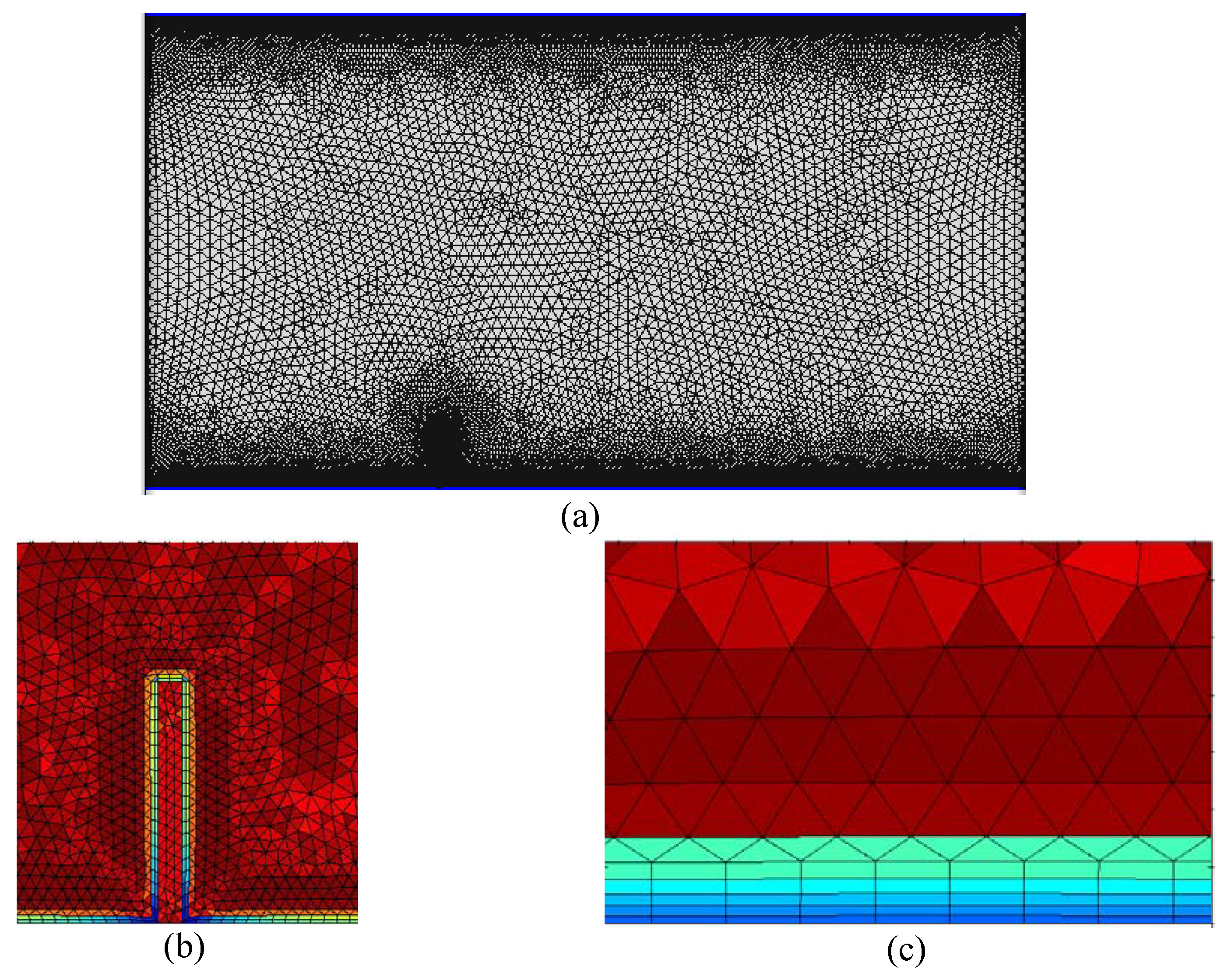
The computational mesh employed in the simulations along with its details around the plate and near the bottom wall are shown in Figure 2. The density of the grid is high near the bottom wall and around the plate surface in order to capture accurately small solid deformations (see Figure 2b,c). The core mesh consists of trihedral elements, except near the bottom wall, where tetrahedral elements were used to resolve the hydrodynamic boundary layer with better accuracy (see Figure 2c). A time step of 0.01 s was employed, which yields an average Courant number of 0.16. The equations were integrated for a total time of 100 s, which is sufficient to establish a steady quasi-periodic state and to analyze the dynamic character of the fluid flow and solid deformation. A mesh independence study was conducted for a dynamic case by approximately doubling the number of finite elements. The grid refinement resulted in differences of less than 3% in the root-mean-squared (r.m.s.) amplitude of the tip displacement.
3. Results
3.1. Rigid Plate
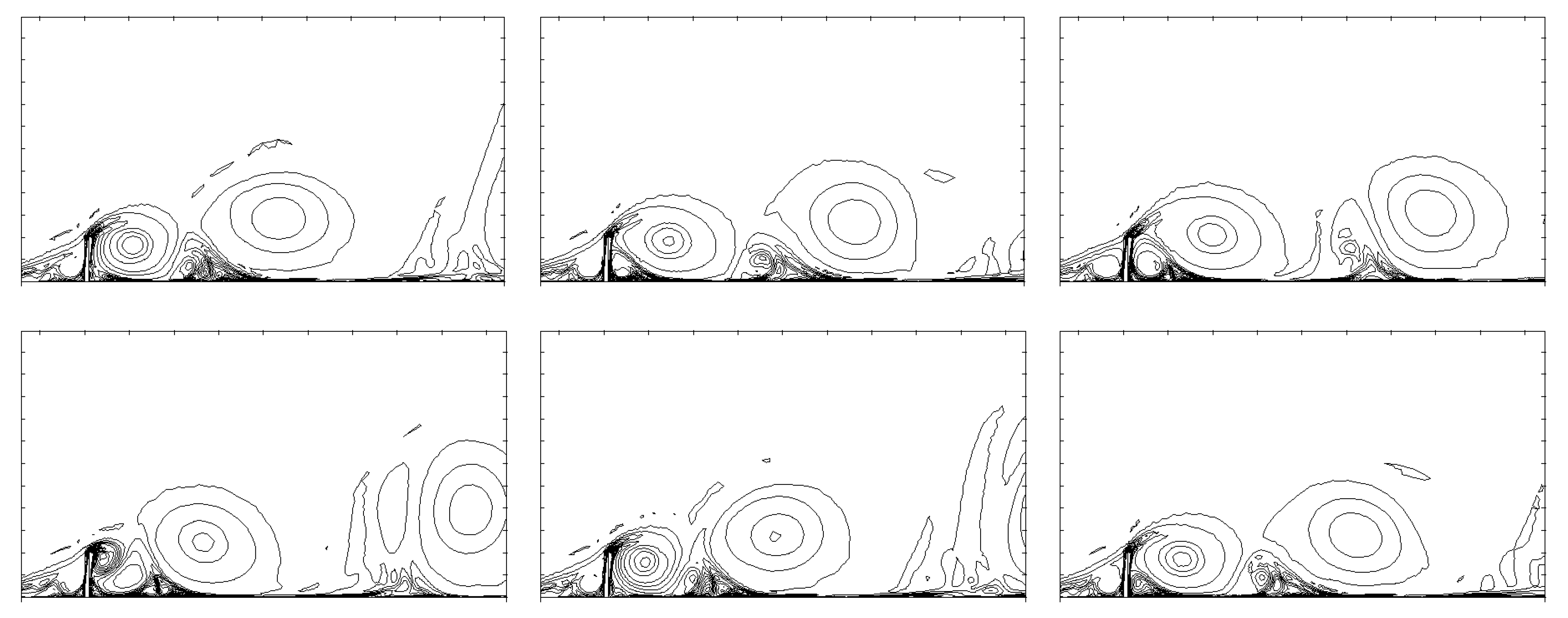
Initially, the flow over a rigid plate was simulated as a reference case for obtaining the frequency of flow instabilities given the scarcity of related information in the literature. Figure 3 shows snapshots of the vorticity distribution at different instants over approximately a flow cycle. It can be clearly seen that the shear layer separating from the free edge rolls up, leading to the formation of large-scale vortices behind the plate. While a “primary” large-scale negative (clockwise) vortex is formed and its circulation increases as it is fed from the shear layer, another smaller positive (anticlockwise) vortex forms at the base of the plate. This “ground” vortex gradually increases in size, until it cuts the supply of vorticity to the primary vortex, which separates from the plate (see the left snapshot in the bottom row of Figure 3). As the primary vortex is convected along the main flow direction, it entrains the ground vortex, which lifts off the bottom and engulfs the primary vortex further downstream. During this lifting process, the ground vortex disintegrates into smaller vortices that become diffused so that the primary vortices generated over subsequent cycles dominate the flow pattern.
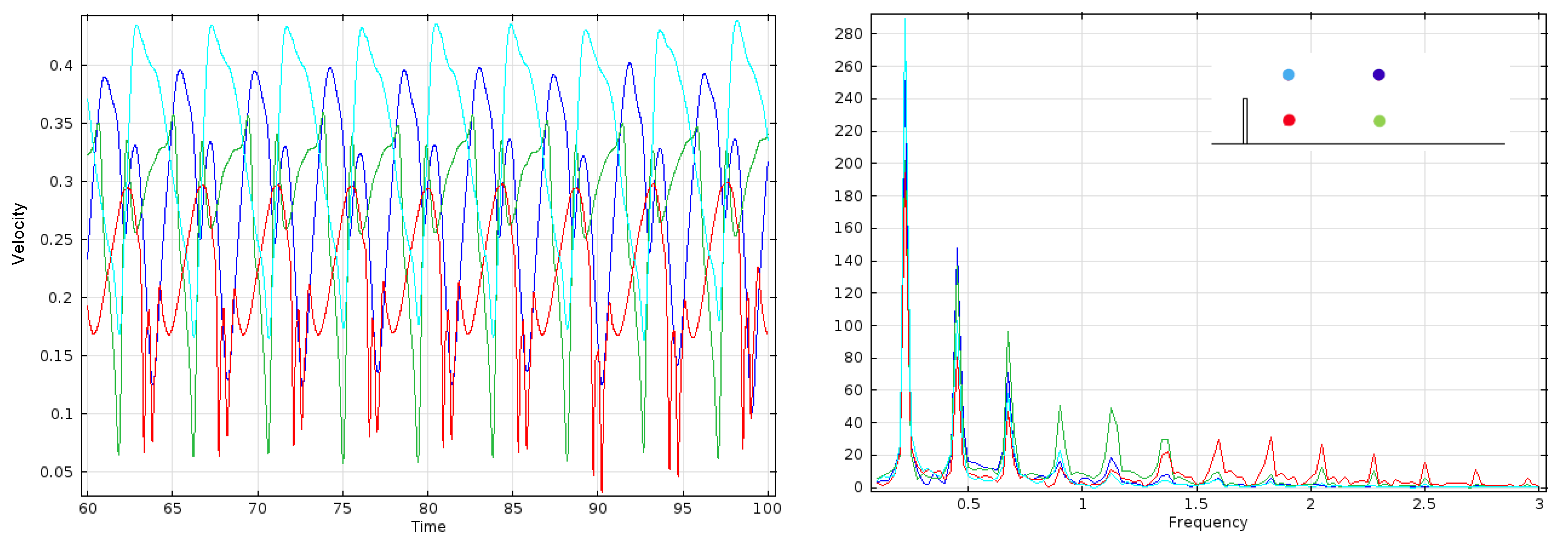
Figure 4 shows the time series of the streamwise velocity fluctuations and the corresponding spectra at four different locations and with respect to the base of the plate . The monitoring points correspond to locations just above and below the shear layer separating from the free edge of the plate. The time series span the last 40 time units of the simulation. There is a clear periodicity in all time series, but the oscillation waveform is quite different at each monitoring point. It can be observed that there are several superharmonics of the main frequency in the spectra that might be attributed to the strongly non-harmonic waveform of the velocity fluctuations induced by the complex process of vortex formation and shedding behind the plate. The dominant peak occurs at Hz, which yields a Strouhal number of . It should be noted that all spectra reported in this paper were obtained by the fast Fourier transform for the last 40 time units of the simulations to avoid transient effects from the initial condition.
As already noted in the Introduction, there are not enough related studies in the published literature to compare the Strouhal number. Fang et al. [45] conducted a 2D numerical study of the flow around a thin plate and found 0.063 at . However, in their study, the ratio of the boundary-layer thickness to the plate height was , whereas in the present study, it is estimated to be at the plate’s location using the Blasius solution. They also found—albeit at a much higher Reynolds number of —that the Strouhal number decreases with , which is consistent with the higher Strouhal number found in the present study. More recently, the nominally two-dimensional flow from a rigid upright fence was investigated by 3D large-eddy simulations [53]. For , it was found that the passage of large-scale eddy structures corresponded to a Strouhal number of 0.08, which is close to the value found in the present study.
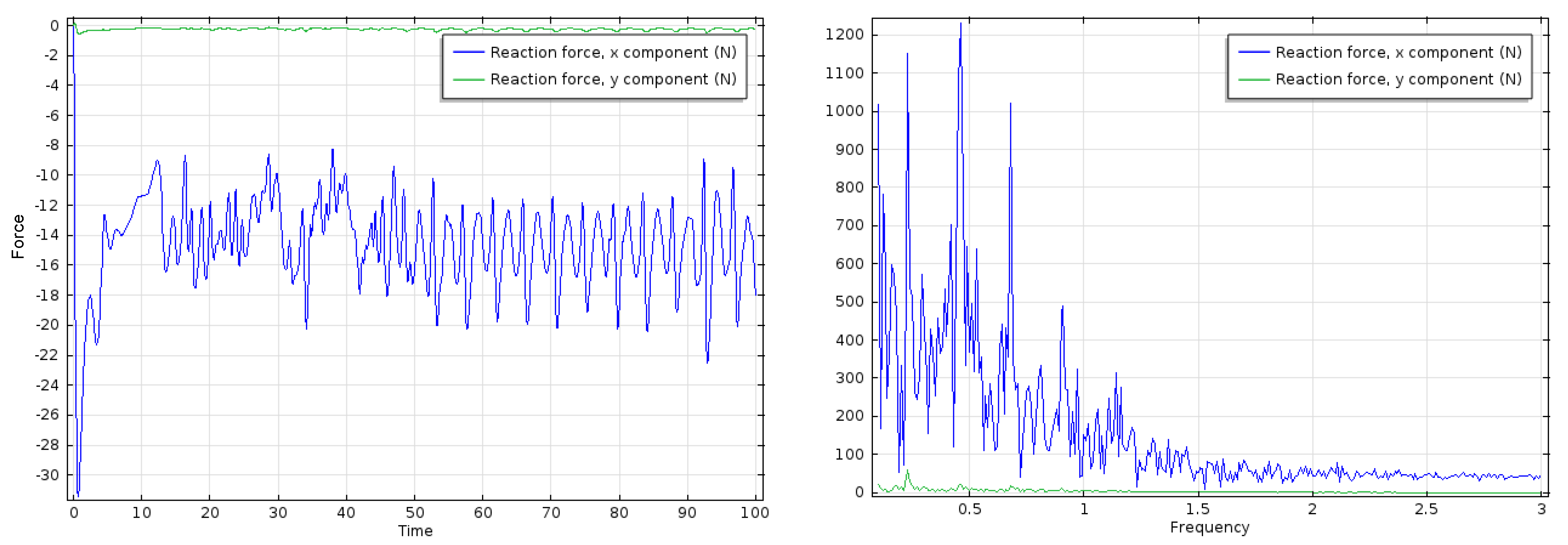
Figure 5 shows time series of the reaction forces exerted by the plate on the fluid in the drag and lift directions from the beginning of the simulation (left plot) and the corresponding spectra computed for the final 40 time units of the simulation (right plot). It can be seen that there is an initial transient period of approximately 50 s until a quasi-periodic state is attained. Both force components exhibit some oscillations induced by the unsteady flow. The drag force exhibits rich spectral content with several peaks. The highest peak in the drag spectrum occurs at twice the frequency of vortex shedding. This might be attributable to the two-step process of vortex formation, i.e., the periodic generation of positive vorticity from the edge and negative vorticity near the base both contribute to the drag force acting on the plate. This resembles the well-known feature that a bluff body that periodically sheds vortices in its wake experiences a drag that has twice the frequency of the lift. On the other hand, the lift force is very small relative to the drag force, and the spectrum of the lift force exhibits a main peak at the frequency of vortex shedding.
3.2. Elastic Plate with
For the simulations with an elastic plate, we aimed to match the fundamental frequency of the structure to the frequency of vortex shedding from the rigid plate ( 0.225 Hz). After initial selection of the material properties of the elastic plate using Equation (1), the structural frequencies were accurately computed via eigen-mode analysis with the finite-element method. When the plate is immersed in fluid, the actual structural frequency will be lower due to the added mass effect [54]. However, here, we use the structural frequency in a vacuum. For a solid density of 7000 kg/m and Young’s modulus of 0.50 GPa, the eigen-mode analysis resulted in Hz, which yields a density ratio of and a reduced velocity of for the test case, which is discussed below.
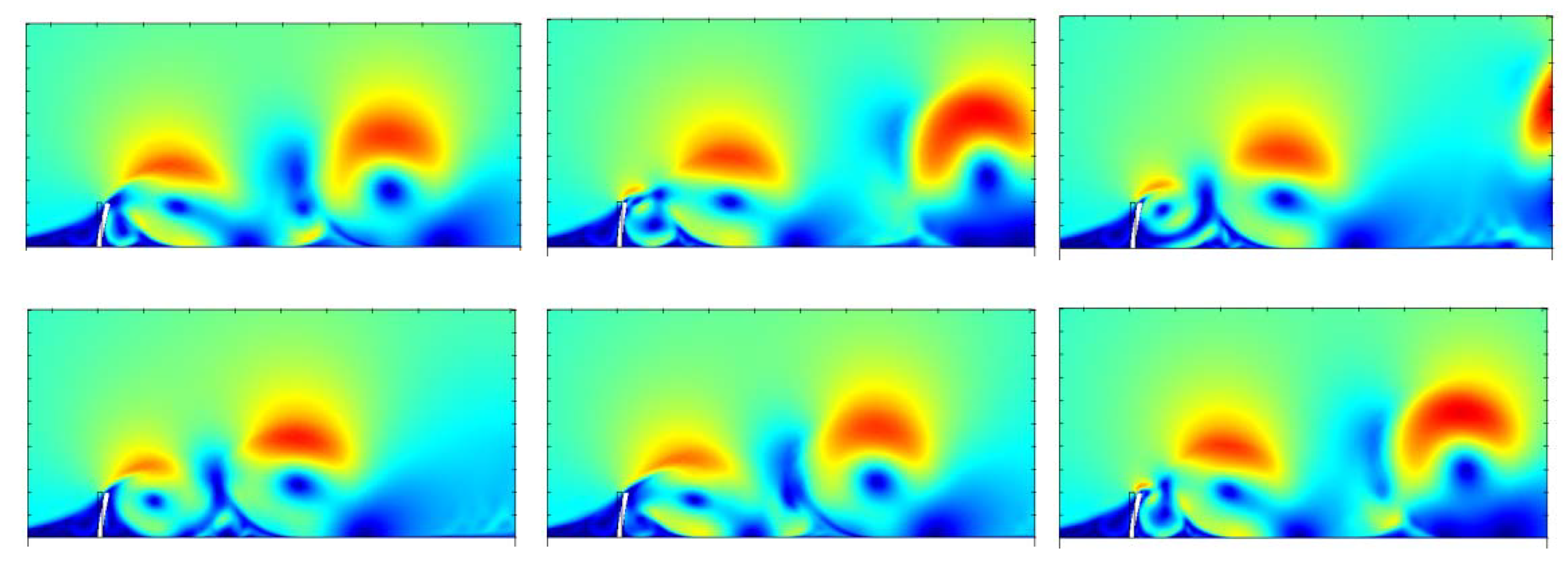
Figure 6 shows snapshots of the vorticity distribution vorticity over the elastic plate at different instants. The process of vortex shedding is similar as in the case of the rigid plate comprising the two-step process of vortex formation from the free edge and from the bottom (cf. Figure 3). However, vorticity concentrations now appear more compact, and vortex motions appear better organized. In addition, the lift-off process of the ground vortex is much clearer for the dynamic case, while the ground vortex remains rather organized after the lift-off. Figure 7 shows the contours of the velocity magnitude, which further illustrate the flow disturbance caused by the regular shedding of vorticity. In both Figure 6 and Figure 7, it can be hardly discerned that the plate gets deflected in the streamwise direction.
Figure 8 shows time series of the streamwise velocity and corresponding spectra corresponding to the last 40 time units of the simulation for the case of a flexible plate at the same monitoring points as for the rigid plate. For the dynamic case, the velocity fluctuations are again close to periodic, but there exist cycle-to-cycle variations. The dominant spectral peak occurs at 0.2275 Hz, which is slightly higher than the frequency of vortex shedding from the rigid plate ( 0.225 Hz). The magnitude of the dominant peak at each monitoring point is lower for the elastic than for the rigid plate, which illustrates that the solid deflection weakens the velocity fluctuations associated with vortex shedding.
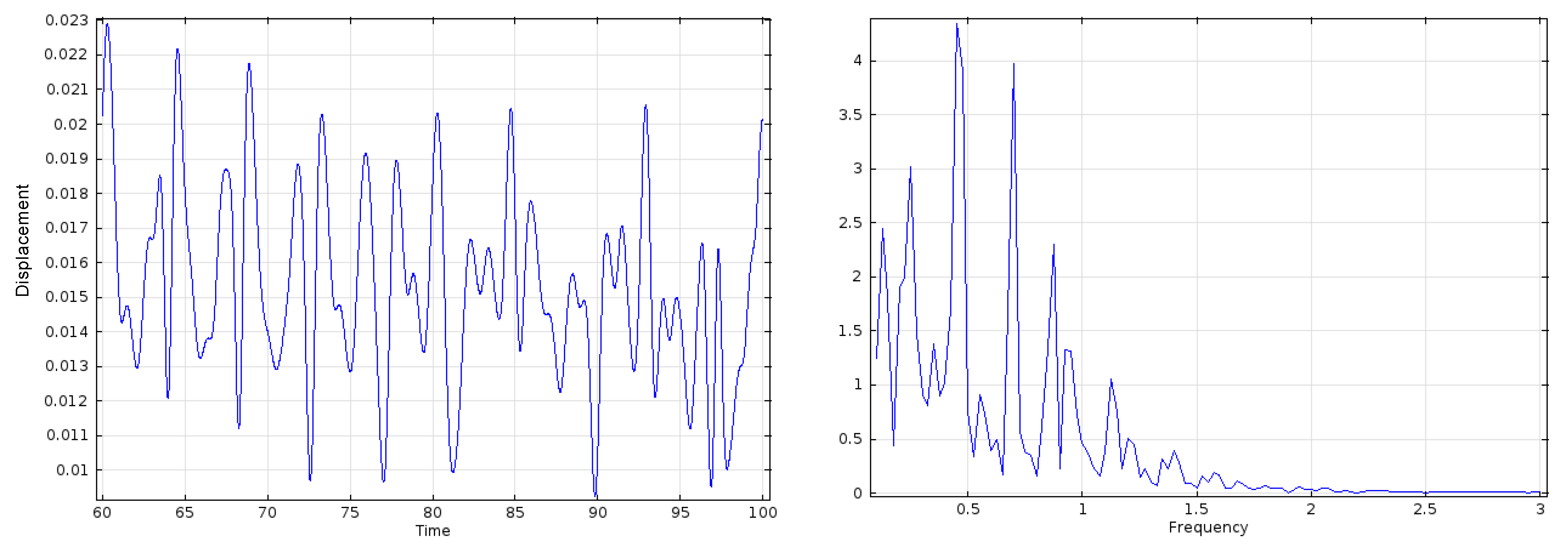
Figure 9 shows the time series of the tip displacement for the last 40 time units of the simulation and the corresponding spectrum. It can be clearly seen that the plate oscillates back and forth with a root-mean-squared amplitude of 0.027H in addition to being deflected by 0.153H on average. In this test case, the tip oscillation is not very regular, and several peaks appear in the tip-displacement spectrum in the right plot. The dominant peak occurs at 0.45 Hz, which is exactly twice the frequency of vortex shedding. The second highest peak occurs at the first superharmonic, while the third highest peak occurs at the first subharmonic. We see that the plate responds to fluid-induced loading by synchronization at twice the vortex shedding frequency when the primary structural frequency is close to the Strouhal frequency of the rigid plate. The synchronization of the vortex shedding to the subharmonic of the oscillation frequency is commensurate to the lock-in phenomenon observed for elastically-mounted rigid and cantilevered elastic circular cylinders undergoing vortex-induced vibration in the streamwise direction [55,56,57]. Interestingly, the same phenomenon is observed here for an elastic plate vibrating along the streamwise direction despite the geometry being substantially different. Therefore, the excitation mechanism can be classified as vortex-induced vibration.
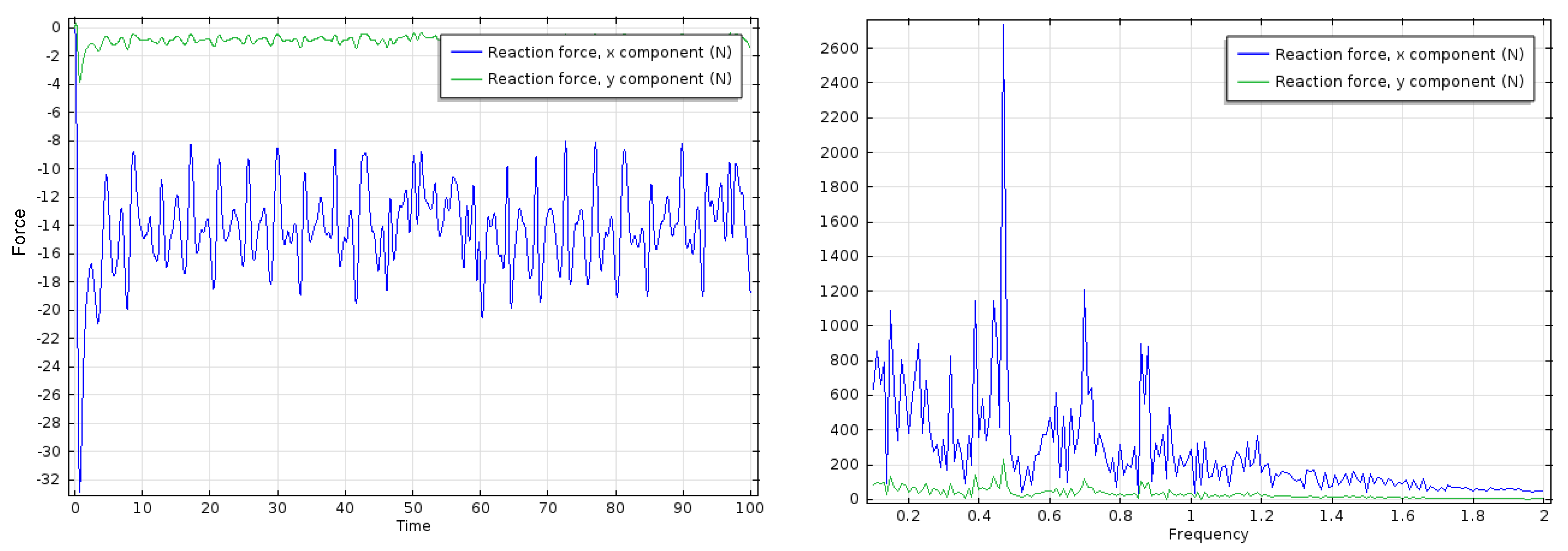
Figure 10 shows time series of the reaction drag and lift forces acting on the elastic plate from the beginning of the simulation (left plot) and corresponding spectra computed for the final 40 time units of the simulation (right plot). In this particular test case, the average drag and the root-mean-squared amplitude of the unsteady drag for the vibrating plate are not much different from their corresponding values for the static plate. However, when the plate is vibrating, the spectrum of the drag force displays a very pronounced peak at 0.45 Hz, i.e., at twice the frequency of vortex shedding, having twice the magnitude of the corresponding peak for the static case. In addition, the dominant peak is much more distinct from other spectral peaks for the elastic plate than for the static one. This might be attributable to additional inertial forces arising from the motion of the plate, which are in-phase with the acceleration and therefore have the same frequency as the motion by default. The lift force increases relative to the static case, but it remains much lower than the drag force. The spectrum of the lift force displays a dominant peak at the main vibration frequency and minor peaks at its superharmonics in contrast to the static plate, in which case the main spectral peak occurs at the shedding frequency.
3.3. Effect of Solid Elasticity and Density
A number of simulations were carried out to investigate the effect of the elasticity and the density of the solid plate on its response. Both parameters affect the structural frequency and thereby the reduced velocity . This provides the opportunity to check if response data could collapse as a function of when either the elasticity or the density is varied. However, it should be noted that variations in the solid density also change the density ratio , whereas variations in the solid elasticity do not change so that independent effects of and on the plate response can also be segregated.
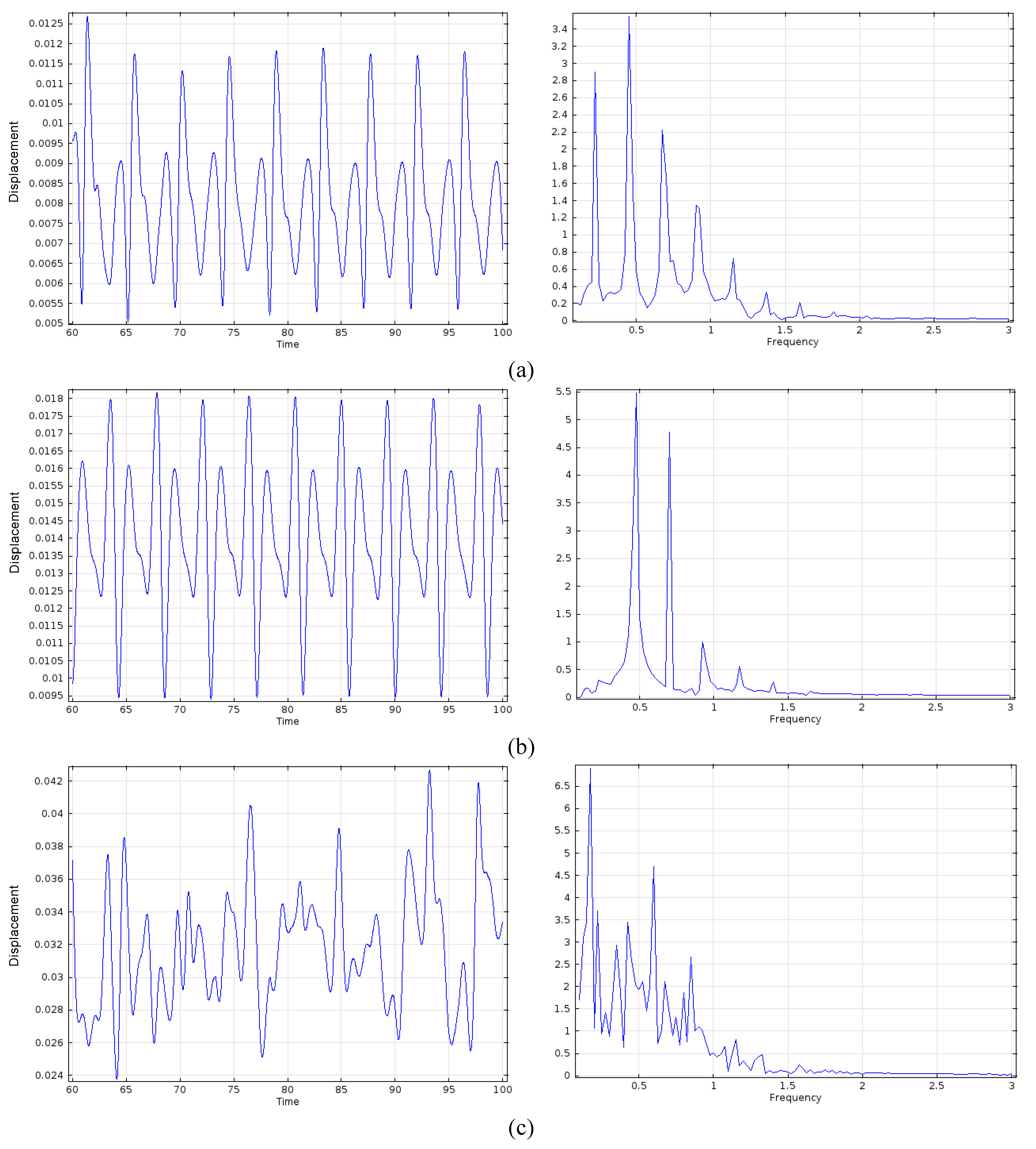
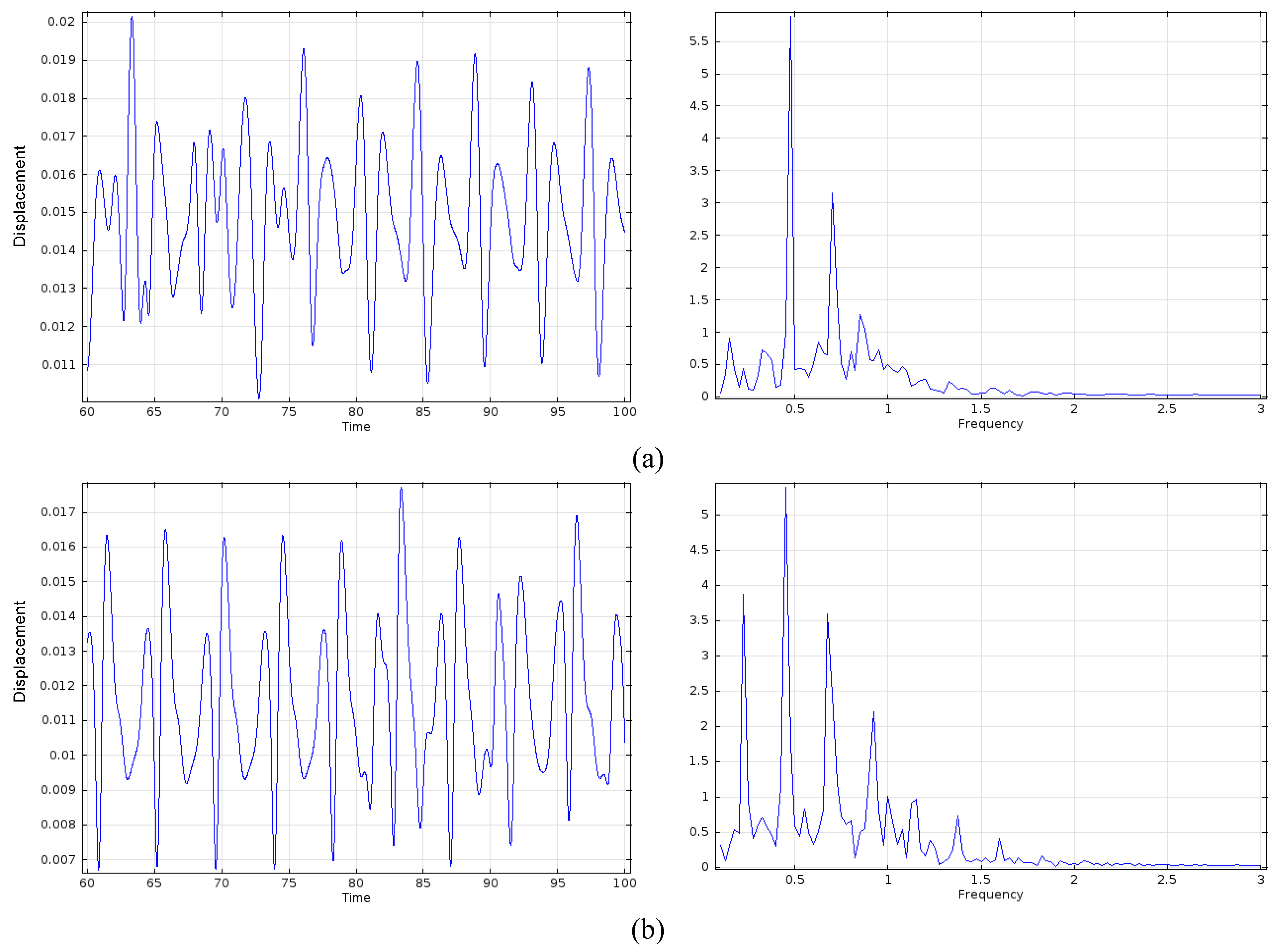
Initially, the Young’s modulus of elasticity was varied from 1 GPa to 0.2 GPa so that was in the range from 8.2 to 18.4, while keeping the density ratio constant at . In all these test cases, the frequency of vortex shedding from the vibrating plate remained close (but not equal) to that from the static plate, , as will be shown in the Discussion. Figure 11 shows time series of the tip displacement and corresponding spectra over the last 40 time units for three test cases. It can be seen that for and 11.1 ( and 0.54 GPa, respectively), the tip displacement becomes almost perfectly periodic with its dominant spectral peak occurring near twice the frequency of vortex shedding of the static plate, i.e., at approximately (Figure 11a,b). It should be noted that the tip vibrated at exactly twice the frequency of vortex shedding, which indicates strong synchronization (or “lock-in”) between the plate motion and the flow for and 11.1. In particular, the test case with GPa was selected so that the structural frequency matches precisely the frequency of vortex shedding from the rigid plate. By decreasing the elasticity further down to 0.2 GPa, the reduced velocity increases to , and the dynamics of the flexible plate and that of the flow become more complex, leading eventually to a chaotic-like response. This is evidence in the time series of tip-displacement oscillations and the fact that the displacement spectra display a broader range of frequencies (Figure 11c). In the latter case, the dominant peak in the displacement spectra is close to the structural frequency rather than that of vortex shedding.
Subsequently, the density of the solid plate was varied while keeping constant the Young’s modulus of elasticity at 0.5 GPa. Figure 12 shows time series of the tip displacement over the last 40 time units for two test cases. For a solid density of 5000 kg/m (), the tip displacement displays a predominant spectral peak close to twice the frequency of vortex shedding from the static plate (Figure 12a). It is interesting to note that for the last 20 time units, the tip oscillations display small-amplitude modulations, although the oscillations appear rather repeatable from cycle to cycle. Another spectral peak appears at approximately , but no peak can be observed at the nominal shedding frequency. A further decrease of the plate density to 3000 kg/m () leads to the re-emergence of a spectral peak close to in addition to the dominant spectral peak at . Higher superharmonics are also present, which could indicate strong synchronization between the tip motion and unsteady flow for .
Generally, the tip displacement displays almost periodic oscillations phase-locked with the unsteady flow when the structural frequency is close to (within the frequency of vortex shedding for the rigid plate, whereas in other cases, there exist amplitude modulations and/or plausible lapses of synchronization. However, the ratio of the frequencies of vortex shedding to the tip oscillation remained fixed at 1:2 in all cases, except for the highest reduced velocity of . The lack of repeatability from cycle to cycle for nominally synchronized cases might be attributable to the turbulent nature of the flow.
4. Discussion
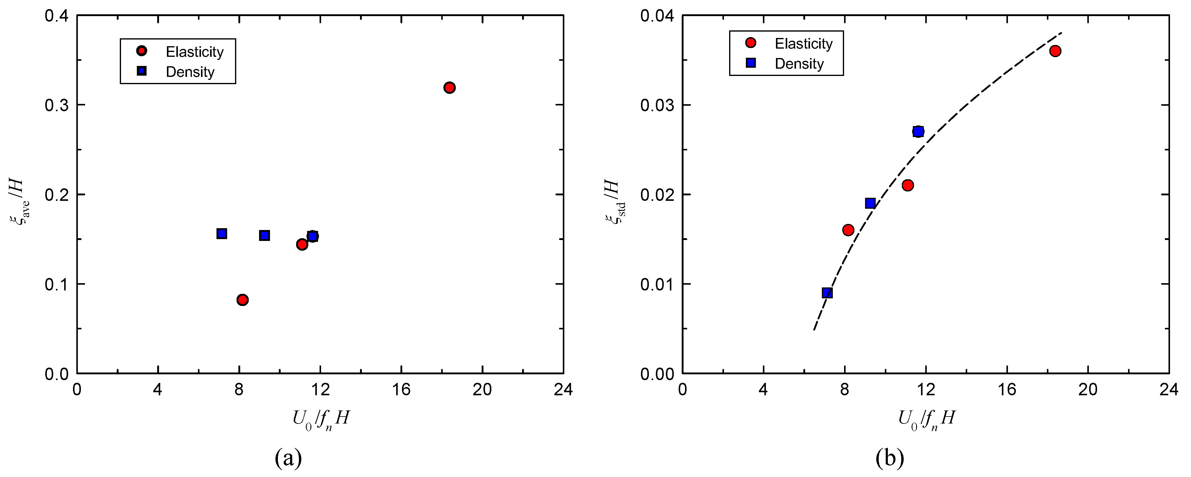
The plate response is summarized in Figure 13, which shows the average tip displacement and the standard deviation of the tip displacement in the streamwise direction for all test cases (values are normalized with the plate height, H). These values were determined from the last 40 time units of the simulations. It should be noted that increases non-linearly with increasing the density or decreasing the elasticity E. It can be seen in Figure 13a that as increases by decreasing E, there is a substantial rise in , i.e., the plate bends more in the streamwise direction, as might be expected. On the other hand, remains almost constant (in fact, there is a marginal decrease) with by increasing . Despite this difference in the average plate deflection, the data appear to collapse when plotted against , as indicated by the dashed curve in Figure 13b, irrespective of whether the structural frequency is varied by changing the elasticity or the density. The data display a nearly four-fold increase from 0.009 to 0.035 with increasing in the range considered in the present study.
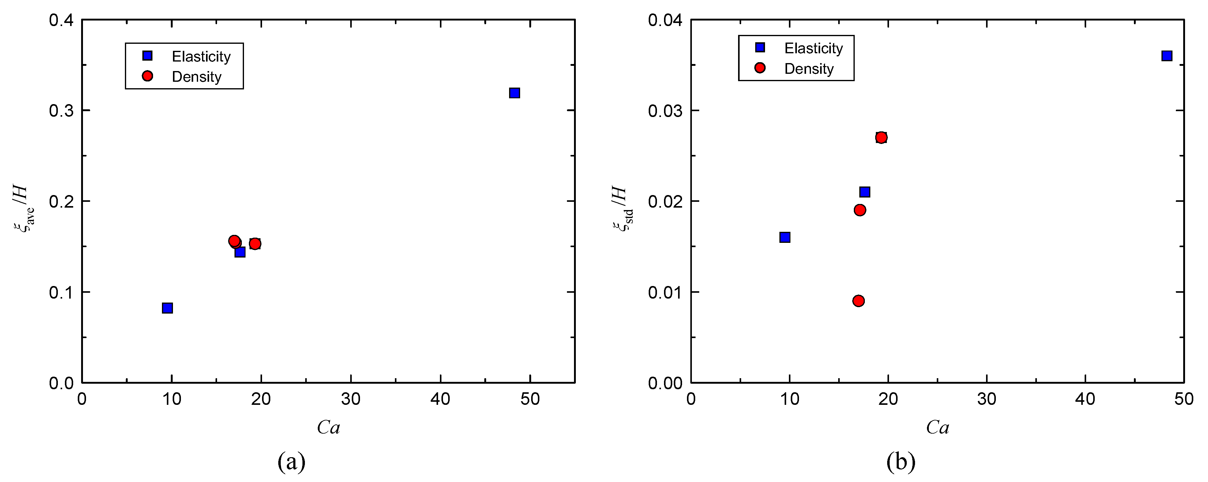
In some previous studies with flexible plates in cross-flow, data for the average deflection were usually compiled as a function of a single dimensionless parameter, the Cauchy number, , where b is the plate width and I is the area moment of inertia of the plate [32,33,58]. The Cauchy number represents the ratio of the drag fluid force to the elastic solid force. These studies focused on the average deflection (sometimes reported in terms of a reconfiguration parameter) as a function of the Cauchy number. Indeed, the present data also collapse fairly well when plotted against , as shown in Figure 14a. In fact, scales almost linearly with . It should be noted that for the two-dimensional configuration considered in the present study, the Cauchy number can be estimated by treating the plate as an elastic beam and is found to be equal to approximately . In contrast, the data for the standard deviation of tip oscillations do not scale with when the elasticity or the density is changed, as shown in Figure 14b. This suggests that the mechanisms responsible for the shape reconfiguration of the flexible plate (average deflection) and its streamwise oscillation are different: the former may be attributable to the mean drag, whereas the latter to the nonlinear coupling of the flow instability with the structural motion.
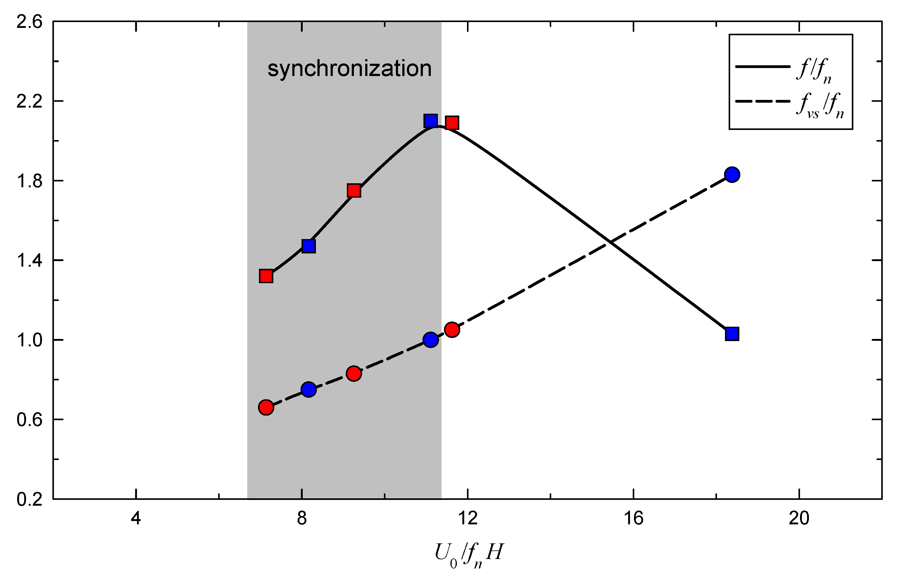
The response frequency of the plate f and the vortex shedding frequency as functions of the reduced velocity are shown together in Figure 15. These frequencies were determined by the dominant spectral peaks, and values were normalized with the natural frequency of the structure, . It should be remembered that is not constant. The continuous lines show b-spline interpolations of the data. It can be noted that increases almost linearly with reduced velocity , irrespective of whether the structural frequency is varied by changing the elasticity or the density. This indicates a fairly constant nominal Strouhal number, . However, a gradual change in the slope can be observed, in particular outside the grey-shaded region marked as “synchronization”, which indicates a slight increase in the nominal Strouhal number. This might be attributable to the fact that the plate bends more as is increased by decreasing the elasticity modulus, and the effective height of the plate becomes lower. If the effective height is , then the shedding frequency should increase with , so that the effective Strouhal number remains approximately constant .
The gray shading in Figure 15 indicates the region where the main frequency of plate vibration synchronizes at twice the frequency of vortex shedding, . This demonstrates that within this region, the excitation mechanism is vortex-induced vibration. However, the synchronization ceases for the two higher values considered. In particular, some coupling must exist between the vortex shedding and the plate motion at ; as shown in Figure 9 and Figure 10, the oscillations of the tip displacement and the drag force are almost perfectly periodic most of the time, but there are some lapses, which is indicative of transitions between synchronization and non-synchronization states. On the other hand, at the highest value of , the tip oscillations become chaotic, as seen in Figure 11c, while the predominant frequency of vibration becomes almost equal to the structural frequency of the plate, i.e., . This could indicate that the vibration resembles flutter, i.e., fluid-elastic instability associated with relatively large amplitude oscillations at the structural frequency beyond some critical reduced velocity [59]. It will be very interesting to examine the plate response in more detail in the range of , which corresponds to the transition between synchronized vortex-induced vibration and chaotic-like flutter vibration, in future work.
Funding
This research received no external funding.
Data Availability Statement
The data generated during this study are available on request to the corresponding author.
Acknowledgments
The author acknowledges the immense help of Athanasios Tsiproupoulos, who carried out the simulations reported in this paper under his supervision.
Conflicts of Interest
The author declares no conflict of interest.
References
- De Langre, E. Effects of Wind on Plants. Annu. Rev. Fluid Mech. 2008, 40, 141–168. [Google Scholar] [CrossRef] [Green Version]
- Tadrist, L.; Julio, K.; Saudreau, M.; de Langre, E. Leaf flutter by torsional galloping: Experiments and model. J. Fluids Struct. 2015, 56, 1–10. [Google Scholar] [CrossRef]
- Song, Z.; Borazjani, I. The Role of Shape and Heart Rate on the Performance of the Left Ventricle. J. Biomech. Eng. 2015, 137, 114501. [Google Scholar] [CrossRef]
- Borazjani, I. Numerical Simulations of Flow around Copepods: Challenges and Future Directions. Fluids 2020, 5, 52. [Google Scholar] [CrossRef] [Green Version]
- Blevins, R.D. Flow-Induced Vibration; Krieger Publishing Company: Malabar, FL, USA, 2001. [Google Scholar]
- Païdoussis, M.P.; Price, S.J.; de Langre, E. Fluid-Structure Interactions: Cross-Flow-Induced Instabilities; Cambridge University Press: New York, NY, USA, 2010. [Google Scholar] [CrossRef]
- Triantafyllou, M.S.; Triantafyllou, G.S.; Yue, D.K.P. Hydrodynamics of Fishlike Swimming. Annu. Rev. Fluid Mech. 2000, 32, 33–53. [Google Scholar] [CrossRef]
- Shi, G.; Xiao, Q.; Zhu, Q. Effects of time-varying flexibility on the propulsion performance of a flapping foil. Phys. Fluids 2020, 32, 121904. [Google Scholar] [CrossRef]
- Borazjani, I. Fluid–structure interaction, immersed boundary-finite element method simulations of bio-prosthetic heart valves. Comput. Methods Appl. Mech. Eng. 2013, 257, 103–116. [Google Scholar] [CrossRef]
- Borazjani, I. A Review of Fluid-Structure Interaction Simulations of Prosthetic Heart Valves. J. Long-Term Eff. Med Implant. 2015, 25, 75–93. [Google Scholar] [CrossRef]
- Akaydin, H.D.; Elvin, N.; Andreopoulos, Y. The performance of a self-excited fluidic energy harvester. Smart Mater. Struct. 2012, 21, 025007. [Google Scholar] [CrossRef]
- Soti, A.K.; Bhardwaj, R.; Sheridan, J. Flow-induced deformation of a flexible thin structure as manifestation of heat transfer enhancement. Int. J. Heat Mass Transf. 2015, 84, 1070–1081. [Google Scholar] [CrossRef] [Green Version]
- Dong, D.; Chen, W.; Shi, S. Coupling Motion and Energy Harvesting of Two Side-by-Side Flexible Plates in a 3D Uniform Flow. Appl. Sci. 2016, 6, 141. [Google Scholar] [CrossRef] [Green Version]
- Gutierrez-Amo, R.; Fernandez-Gamiz, U.; Errasti, I.; Zulueta, E. Computational Modelling of Three Different Sub-Boundary Layer Vortex Generators on a Flat Plate. Energies 2018, 11, 3107. [Google Scholar] [CrossRef] [Green Version]
- Jin, Y.; Kim, J.T.; Hong, L.; Chamorro, L.P. Flow-induced oscillations of low-aspect-ratio flexible plates with various tip geometries. Phys. Fluids 2018, 30, 097102. [Google Scholar] [CrossRef]
- Allen, J.; Smits, A. Energy Harvesting Eel. J. Fluids Struct. 2001, 15, 629–640. [Google Scholar] [CrossRef] [Green Version]
- Young, J.; Lai, J.C.; Platzer, M.F. A review of progress and challenges in flapping foil power generation. Prog. Aerosp. Sci. 2014, 67, 2–28. [Google Scholar] [CrossRef]
- McCarthy, J.; Watkins, S.; Deivasigamani, A.; John, S. Fluttering energy harvesters in the wind: A review. J. Sound Vib. 2016, 361, 355–377. [Google Scholar] [CrossRef]
- Sun, H.; Ma, C.; Bernitsas, M.M. Hydrokinetic power conversion using Flow Induced Vibrations with cubic restoring force. Energy 2018, 153, 490–508. [Google Scholar] [CrossRef]
- Sun, H.; Bernitsas, M.M. Bio-Inspired adaptive damping in hydrokinetic energy harnessing using flow-induced oscillations. Energy 2019, 176, 940–960. [Google Scholar] [CrossRef] [Green Version]
- Binyet, E.M.; Chang, J.Y.; Huang, C.Y. Flexible Plate in the Wake of a Square Cylinder for Piezoelectric Energy Harvesting—Parametric Study Using Fluid–Structure Interaction Modeling. Energies 2020, 13, 2645. [Google Scholar] [CrossRef]
- Malefaki, I.; Konstantinidis, E. Assessment of a Hydrokinetic Energy Converter Based on vortex Induced Angular Oscillations of a Cylinder. Energies 2020, 13, 717. [Google Scholar] [CrossRef] [Green Version]
- Xu, W.; Yang, M.; Wang, E.; Sun, H. Performance of single-cylinder VIVACE converter for hydrokinetic energy harvesting from flow-induced vibration near a free surface. Ocean. Eng. 2020, 218, 108168. [Google Scholar] [CrossRef]
- Shelley, M.J.; Zhang, J. Flapping and Bending Bodies Interacting with Fluid Flows. Annu. Rev. Fluid Mech. 2011, 43, 449–465. [Google Scholar] [CrossRef] [Green Version]
- Cisonni, J.; Lucey, A.D.; Elliott, N.S.; Heil, M. The stability of a flexible cantilever in viscous channel flow. J. Sound Vib. 2017, 396, 186–202. [Google Scholar] [CrossRef] [Green Version]
- Tavallaeinejad, M.; Païdoussis, M.P.; Legrand, M.; Kheiri, M. Instability and the post-critical behaviour of two-dimensional inverted flags in axial flow. J. Fluid Mech. 2020, 890, A14. [Google Scholar] [CrossRef]
- Tavallaeinejad, M.; Salinas, M.F.; Païdoussis, M.P.; Legrand, M.; Kheiri, M.; Botez, R.M. Dynamics of inverted flags: Experiments and comparison with theory. J. Fluids Struct. 2021, 101, 103199. [Google Scholar] [CrossRef]
- Alben, S.; Shelley, M.; Zhang, J. Drag reduction through self-similar bending of a flexible body. Nature 2002, 420, 479–481. [Google Scholar] [CrossRef] [PubMed]
- Yang, X.; Liu, M.; Peng, S. Smoothed particle hydrodynamics and element bending group modeling of flexible fibers interacting with viscous fluids. Phys. Rev. E 2014, 90, 063011. [Google Scholar] [CrossRef] [Green Version]
- Henriquez, S.; Barrero-Gil, A. Reconfiguration of flexible plates in sheared flow. Mech. Res. Commun. 2014, 62, 1–4. [Google Scholar] [CrossRef]
- Leclercq, T.; de Langre, E. Drag reduction by elastic reconfiguration of non-uniform beams in non-uniform flows. J. Fluids Struct. 2016, 60, 114–129. [Google Scholar] [CrossRef]
- Barois, T.; de Langre, E. Flexible body with drag independent of the flow velocity. J. Fluid Mech. 2013, 735, R2. [Google Scholar] [CrossRef] [Green Version]
- Barsu, S.; Doppler, D.; Jerome, J.J.S.; Rivière, N.; Lance, M. Drag measurements in laterally confined 2D canopies: Reconfiguration and sheltering effect. Phys. Fluids 2016, 28, 107101. [Google Scholar] [CrossRef] [Green Version]
- Tian, F.B.; Dai, H.; Luo, H.; Doyle, J.F.; Rousseau, B. Fluid–structure interaction involving large deformations: 3D simulations and applications to biological systems. J. Comput. Phys. 2014, 258, 451–469. [Google Scholar] [CrossRef] [Green Version]
- Basting, S.; Quaini, A.; Čanić, S.; Glowinski, R. Extended ALE Method for fluid–structure interaction problems with large structural displacements. J. Comput. Phys. 2017, 331, 312–336. [Google Scholar] [CrossRef] [Green Version]
- Bano, T.; Hegner, F.; Heinrich, M.; Schwarze, R. Investigation of Fluid-Structure Interaction Induced Bending for Elastic Flaps in a Cross Flow. Appl. Sci. 2020, 10, 6177. [Google Scholar] [CrossRef]
- Dey, A.A.; Modarres-Sadeghi, Y.; Rothstein, J.P. Viscoelastic flow-induced oscillations of a cantilevered beam in the crossflow of a wormlike micelle solution. J. Non-Newton. Fluid Mech. 2020, 286, 104433. [Google Scholar] [CrossRef]
- Plate, E.J. The aerodynamics of shelter belts. Agric. Meteorol. 1971, 8, 203–222. [Google Scholar] [CrossRef]
- Raine, J.; Stevenson, D. Wind protection by model fences in a simulated atmospheric boundary layer. J. Wind. Eng. Ind. Aerodyn. 1977, 2, 159–180. [Google Scholar] [CrossRef]
- Perera, M. Shelter behind two-dimensional solid and porous fences. J. Wind. Eng. Ind. Aerodyn. 1981, 8, 93–104. [Google Scholar] [CrossRef]
- Lee, S.J.; Kim, H.B. Laboratory measurements of velocity and turbulence field behind porous fences. J. Wind. Eng. Ind. Aerodyn. 1999, 80, 311–326. [Google Scholar] [CrossRef]
- Dong, Z.; Luo, W.; Qian, G.; Lu, P.; Wang, H. A wind tunnel simulation of the turbulence fields behind upright porous wind fences. J. Arid. Environ. 2010, 74, 193–207. [Google Scholar] [CrossRef]
- Liu, B.; Qu, J.; Zhang, W.; Tan, L.; Gao, Y. Numerical evaluation of the scale problem on the wind flow of a windbreak. Sci. Rep. 2014, 4, 6619. [Google Scholar] [CrossRef] [Green Version]
- Pieris, S.; Tuna, B.; Yarusevych, S.; Peterson, S. Flow development upstream of a fence. Int. J. Heat Fluid Flow 2020, 82, 108565. [Google Scholar] [CrossRef]
- Fang, F.M.; Hsieh, W.D.; Jong, S.W.; She, J.J. Unsteady Turbulent Flow Past Solid Fence. J. Hydraul. Eng. 1997, 123, 560–565. [Google Scholar] [CrossRef]
- Hwang, R.R.; Chow, Y.; Peng, Y. Numerical study of turbulent flow over two-dimensional surface-mounted ribs in a channel. Int. J. Numer. Methods Fluids 1999, 31, 767–785. [Google Scholar] [CrossRef]
- Fragos, V.; Psychoudaki, S.; Malamataris, N. Two-dimensional numerical simulation of vortex shedding and flapping motion of turbulent flow around a rib. Comput. Fluids 2012, 69, 108–121. [Google Scholar] [CrossRef]
- Siller, H.; Fernholz, H. Control of the separated flow downstream of a two-dimensional fence by low-frequency forcing. Appl. Sci. Res. 1996, 57, 309–318. [Google Scholar] [CrossRef]
- Orellano, A.; Wengle, H. Numerical simulation (DNS and LES) of manipulated turbulent boundary layer flow over a surface-mounted fence. Eur. J. Mech. B/Fluids 2000, 19, 765–788. [Google Scholar] [CrossRef]
- Blevins, R.D. Formulas for Dynamics, Acoustics and Vibration; John Wiley & Sons, Ltd.: Chichester, UK, 2016. [Google Scholar] [CrossRef]
- Eloy, C.; Souilliez, C.; Schouveiler, L. Flutter of a rectangular plate. J. Fluids Struct. 2007, 23, 904–919. [Google Scholar] [CrossRef]
- Launder, B.; Spalding, D. The numerical computation of turbulent flows. Comput. Methods Appl. Mech. Eng. 1974, 3, 269–289. [Google Scholar] [CrossRef]
- Basnet, K. Flow around Porous Barriers: Fundamental Flow Physics and Applications. Ph.D. Thesis, University of Iowa, Iowa City, IA, USA, 2015. Available online: http://ir.uiowa.edu/etd/1824 (accessed on 28 November 2016).
- Chen, G.; Alam, M.M.; Zhou, Y. Dependence of added mass on cylinder cross-sectional geometry and orientation. J. Fluids Struct. 2020, 99, 103142. [Google Scholar] [CrossRef]
- Okajima, A.; Nakamura, A.; Kosugi, T.; Uchida, H.; Tamaki, R. Flow-induced in-line oscillation of a circular cylinder. Eur. J. Mech. B Fluids 2004, 23, 115–125. [Google Scholar] [CrossRef]
- Sherwood, J.; Dusting, J.; Konstantinidis, E.; Balabani, S. Flow-Induced Streamwise Vibration of a Flexibly-Mounted Cantilevered Cylinder in Steady and Pulsating Crossflow. In Proceedings of the ASME 2009 Pressure Vessels and Piping Conference, Prague, Czech Republic, 26–30 July 2009; Volume 4: Fluid-Structure Interaction, pp. 203–210. [Google Scholar] [CrossRef]
- Konstantinidis, E. On the response and wake modes of a cylinder undergoing streamwise vortex induced vibration. J. Fluids Struct. 2014, 45, 256–262. [Google Scholar] [CrossRef]
- Jin, Y.; Kim, J.T.; Fu, S.; Chamorro, L.P. Flow-induced motions of flexible plates: Fluttering, twisting and orbital modes. J. Fluid Mech. 2019, 864, 273–285. [Google Scholar] [CrossRef]
- Tavallaeinejad, M.; Païdoussis, M.P.; Flores Salinas, M.; Legrand, M.; Kheiri, M.; Botez, R.M. Flapping of heavy inverted flags: A fluid-elastic instability. J. Fluid Mech. 2020, 904, R5. [Google Scholar] [CrossRef]
Figure 1.
Schematic showing the flow domain and the boundary conditions employed in the simulations.
Figure 1.
Schematic showing the flow domain and the boundary conditions employed in the simulations.

Figure 2.
The computational mesh (a), detail of the mesh around the plate (b), and detail of the mesh near the bottom solid boundary (c).
Figure 2.
The computational mesh (a), detail of the mesh around the plate (b), and detail of the mesh near the bottom solid boundary (c).

Figure 3.
Snapshots of the vorticity distribution around a rigid plate at different instants going from left to right, then below, which show the flow development over approximately a cycle of vortex shedding.
Figure 3.
Snapshots of the vorticity distribution around a rigid plate at different instants going from left to right, then below, which show the flow development over approximately a cycle of vortex shedding.

Figure 4.
Time series of the streamwise velocity (left plot) and corresponding spectra (right plot) at different locations for a rigid plate. The insert shows the monitoring locations of the velocity.
Figure 4.
Time series of the streamwise velocity (left plot) and corresponding spectra (right plot) at different locations for a rigid plate. The insert shows the monitoring locations of the velocity.

Figure 5.
Time series of the reaction drag and lift forces acting on the plate (left plot) and corresponding spectra (right plot) for a rigid plate.
Figure 5.
Time series of the reaction drag and lift forces acting on the plate (left plot) and corresponding spectra (right plot) for a rigid plate.

Figure 6.
Snapshots of the vorticity distribution around a vibrating elastic plate at different instants from left to right, then below for and .
Figure 6.
Snapshots of the vorticity distribution around a vibrating elastic plate at different instants from left to right, then below for and .

Figure 7.
Contours of the velocity magnitude around a vibrating elastic plate at different instants going from left to right, then below for and .
Figure 7.
Contours of the velocity magnitude around a vibrating elastic plate at different instants going from left to right, then below for and .

Figure 8.
Time series of the streamwise velocity (left plot) and corresponding spectra (right plot) at different locations downstream of the elastic plate for and .
Figure 8.
Time series of the streamwise velocity (left plot) and corresponding spectra (right plot) at different locations downstream of the elastic plate for and .

Figure 9.
Time series of the tip displacement of the elastic plate (left plot) and the corresponding spectrum (right plot) for and .
Figure 9.
Time series of the tip displacement of the elastic plate (left plot) and the corresponding spectrum (right plot) for and .

Figure 10.
Time series of the reaction drag and lift forces acting on the elastic plate (left plot) and corresponding spectra (right plot) for and .
Figure 10.
Time series of the reaction drag and lift forces acting on the elastic plate (left plot) and corresponding spectra (right plot) for and .

Figure 11.
Time series of the tip displacement of the vibrating plate (left column) and corresponding spectra (right column) at different elasticity values (a) GPa (), (b) GPa (), and (c) GPa () and constant density ratio .
Figure 11.
Time series of the tip displacement of the vibrating plate (left column) and corresponding spectra (right column) at different elasticity values (a) GPa (), (b) GPa (), and (c) GPa () and constant density ratio .

Figure 12.
Time series of the tip displacement of the vibrating plate (left column) and corresponding spectra (right column) for constant elasticity ( GPa) and different solid densities: (a) kg/m () and (b) kg/m ().
Figure 12.
Time series of the tip displacement of the vibrating plate (left column) and corresponding spectra (right column) for constant elasticity ( GPa) and different solid densities: (a) kg/m () and (b) kg/m ().

Figure 13.
The plate response as function of the reduced velocity : (a) average tip displacement and (b) standard deviation of the tip displacement . The reduced velocity is varied by changing either the density or the elasticity of the solid plate; other parameters kept fixed, as indicated in the legend.

Figure 14.
The plate response as function of the Cauchy number : (a) average tip displacement and (b) standard deviation of the tip displacement . The Cauchy number is varied by changing either the density or the elasticity of the solid plate; other parameters kept fixed, as indicated in the legend.

Figure 15.
The response frequency of the plate and the frequency of vortex shedding as functions of the reduced velocity : The reduced velocity is varied by changing either the density (blue symbols) or the elasticity (red symbols) of the solid plate.
Figure 15.
The response frequency of the plate and the frequency of vortex shedding as functions of the reduced velocity : The reduced velocity is varied by changing either the density (blue symbols) or the elasticity (red symbols) of the solid plate.


Table 1.
Geometrical, fluid, and solid properties employed in the present study.
| Fluid | Density, | 1000 kg/m |
| Viscosity, | 0.001 Pa·s | |
| Velocity, | 0.25 m/s | |
| Solid | Height, H | 0.1 m |
| Thickness | 0.01 m | |
| Poisson’s ratio, | 0.33 | |
| Density, | 3000–7000 kg/m | |
| Young’s modulus, E | 0.2–1.0 GPa |
Publisher’s Note: MDPI stays neutral with regard to jurisdictional claims in published maps and institutional affiliations. |
© 2021 by the author. Licensee MDPI, Basel, Switzerland. This article is an open access article distributed under the terms and conditions of the Creative Commons Attribution (CC BY) license (http://creativecommons.org/licenses/by/4.0/).
Share and Cite
MDPI and ACS Style
Konstantinidis, E. Cross-Flow-Induced Vibration of an Elastic Plate. Fluids 2021, 6, 82. https://0-doi-org.brum.beds.ac.uk/10.3390/fluids6020082
AMA Style
Konstantinidis E. Cross-Flow-Induced Vibration of an Elastic Plate. Fluids. 2021; 6(2):82. https://0-doi-org.brum.beds.ac.uk/10.3390/fluids6020082
Chicago/Turabian StyleKonstantinidis, Efstathios. 2021. "Cross-Flow-Induced Vibration of an Elastic Plate" Fluids 6, no. 2: 82. https://0-doi-org.brum.beds.ac.uk/10.3390/fluids6020082